All articles published by MDPI are made immediately available worldwide under an open access license. No special
permission is required to reuse all or part of the article published by MDPI, including figures and tables. For
articles published under an open access Creative Common CC BY license, any part of the article may be reused without
permission provided that the original article is clearly cited. For more information, please refer to
https://www.mdpi.com/openaccess.
Feature papers represent the most advanced research with significant potential for high impact in the field. A Feature
Paper should be a substantial original Article that involves several techniques or approaches, provides an outlook for
future research directions and describes possible research applications.
Feature papers are submitted upon individual invitation or recommendation by the scientific editors and must receive
positive feedback from the reviewers.
Editor’s Choice articles are based on recommendations by the scientific editors of MDPI journals from around the world.
Editors select a small number of articles recently published in the journal that they believe will be particularly
interesting to readers, or important in the respective research area. The aim is to provide a snapshot of some of the
most exciting work published in the various research areas of the journal.
The fruitfulness of the method of a non-equilibrium statistical operator (NSO) and generalized linear response theory is demonstrated calculating the permittivity, dynamical conductivity, absorption coefficient, and dynamical collision frequency of plasmas in the degenerate, metallic state as well as classical plasmas. A wide range of plasma parameters is considered, and a wide range of frequencies of laser radiation acting on such plasmas is treated. New analytical expressions for the plasma response are obtained by this method, and several limiting cases are discussed.
The non-equilibrium quantum statistical operator (NSO) was proposed by D.N. Zubarev [1], and its 100-year anniversary was celebrated recently. The NSO method is an important step in working out a unified, general approach to nonequilibrium phenomena such as transport and relaxation processes. Different approaches to describe nonequilibrium processes, such as kinetic theory, linear response theory, and quantum master equations, are obtained within a very general approach, after specifying the relevant degrees of freedom that characterize the non-equilibrium state of the system. Recent reviews of the NSO method and its applications can be found, e.g., in [2,3,4,5,6].
The NSO method has been successfully applied to many problems related to the transport and optical properties of charged particle systems, such as warm dense matter (WDM). Reviews of the calculations of dynamical response of dense plasmas are found, e.g., in [7,8]. A main advantage of the approach is that special approaches, valid in limiting cases, can be generalized to describe more complex situations. For instance, kinetic theory has been worked out for low-density systems where the single-particle distribution function is relevant to describing the non-equilibrium state of the system, and correlations can be neglected. In contrast, linear response theory has been worked out to describe systems at arbitrary densities, but near thermodynamical equilibrium. A unified theory that covers both limiting cases has been worked out using the NSO method, see [9]. In particular, the correct frequency dependence of the response functions has been found, in contrast to conventional kinetic theory. A further advantage of the approach is that non-equilibrium properties of quantum as well as classical plasmas can be considered consistently on the same footing. Altogether, the NSO method allows one to study the transport and optical properties of plasmas at arbitrary densities and temperatures, including the region of WDM where correlations are strong, in particular between ions, and where the electrons become degenerate. The response to classical Maxwell fields, represented by a time-dependent external field in the Hamiltonian, can be investigated in a wide range of frequencies of the external field. This refers also to the response of WDM that is irradiated by laser fields, in particular the frequency-dependent absorption coefficient. To include a spontaneous emission of photons, a quantum description of the Maxwell fields is necessary.
In this paper, we present briefly the NSO method and its application to the permittivity of metallic plasmas, which is described by a Hamiltonian accounting for electron–phonon interactions and Umklapp processes, as well as the application to the permittivity of plasmas without a long-range order of ions, which is described by a Hamiltonian accounting for electron–ion and electron–electron interactions. We continue our previous investigations to work out a systematic quantum statistical approach to the response properties of WDM [10,11,12,13,14] with an application to aluminum, considering additional processes of interaction in the strongly coupled Coulomb system. We derive analytical expressions for the dynamical collision frequency and related quantities, in particular the absorption coefficient. The behavior of these response properties, such as temperature dependence and frequency dependence, is discussed in special limiting cases.
These results are of interest for the investigation of material at extremal conditions, e.g., high-particle and high-energy densities. If a solid metallic target is irradiated by powerful laser pulses, the electron component of such a target undergoes modifications of its properties, changing from the state of a metallic “plasma” to a state of a classical non-degenerate plasma. This transition of the electron system from a degenerate state to a classical behavior is consistently described in our approach. In addition, the ion system may change from a solid state, where the ion positions are strongly correlated forming a lattice, to a liquid or a plasma state, where the long-range order of ion positions is destructed. In the present work, we neglect the short-range order of the ion system in the liquid or plasma state, so that the electron–ion interaction is considered as independent scattering at the individual ions. For the electron–ion interaction in the solid state of matter, the coherent part of multiple scattering by the ionic lattice leads to the formation of electron band (Bloch) states. The deviation of ions from the lattice position is described as phonon excitation, and the electron–phonon interaction together with Umklapp processes is considered in this work as responsible for the dynamical conductivity of the solid metal, in addition to electron–electron collisions. Such transitions from collective electron–phonon interactions in a solid to individual electron–ion interactions in the disordered ion configuration directly opens up the question about the switching between the respective Hamiltonians. A more general approach is possible using the concept of the dynamical structure factor which reflects not only the configuration of the ions but also the dynamical behavior, including collective excitations, of the ion system. This problem, however, requires a separate investigation and is not considered in the present work.
With respect to the application to aluminum plasmas, recent experiments in the WDM region [15,16] to measure the dynamical conductivity are also treated by density-functional theory (DFT) for electrons combined with molecular dynamics (MD) calculations for the ions [17]. These calculations have the advantage that optimal single-electron orbitals are calculated, and these orbitals reflect the electron structure of the aluminum ion, improving our effective electron–ion () interaction potential. In addition, the static ionic structure factor is calculated so that a short-range order in the liquid or plasma phase is implemented in the calculation of the dynamical conductivity. However, the choice of the density functional for the correlation energy remains an open problem of these DFT-MD calculations. A shortcoming of the DFT-MD approach is that electron–electron () collisions are not properly included in this mean-field theory, in contrast to our generalized linear response approach, where the contribution of collisions is taken into account, see also [18].
A systematic improvement of our approach is the use of optimal single-electron orbits and interaction potentials. In addition, the dynamical ion structure factor that causes not only multiple scattering of the electrons, but also the excitation of the ion system, in particular phonons, should be considered in a systematic approach. These improvements in our calculations that establish a closer connection to DFT-MD simulations are a subject of future work.
2. A Brief Description of the Method
The plasma permittivity of an electromagnetic field with the frequency is directly related to the dynamical conductivity according to or, using Gauss units instead of SI units, as follows:
Here and below we consider isotropic media in the case of weak spacial dispersion or the long-wavelength (with respect to plasma perturbations) limit. In this case, the permittivity does not depend on the wave vector of perturbations. The longitudinal permittivity coincides with the transverse one: [19].
For the calculation of , one should determine the (quantum) statistically averaged electric current, arising as the system’s response to external electromagnetic fields. Such calculation can be done using the NSO , which can be constructed as a sum of the so-called relevant statistical operator describing the quasi-equilibrium and the irrelevant statistical operator , which represents the nonequilibrium contribution.
The relevant statistical operator is introduced as a generalized Gibbs ensemble, derived from the principle of the maximum of entropy:
where is the Hamiltonian of the system. is the particle number operator, where and are the creation and annihilation operators of the electrons in state p. For the chosen set of relevant observables , we request
meaning that the observed statistical averages at time t are correctly reproduced by the averages with the relevant statistical operator . The Lagrange parameters are then determined by the set of requested expressions (3) as response parameters. Similar conditions on and determine as chemical potential and , respectively, where is the electron temperature. (We give the temperature in energy units, , instead of SI units where .)
If (i.e., an empty set of relevant observables), the operator (2) is identical with the statistical operator for the grand canonical ensemble [3]. In that case, the well-known Kubo formula [20] for the electrical conductivity follows immediately [4,5].
The choice of relevant observables can be arbitrary. Different choices lead to the same results if non-perturbative approaches such as infinite diagram summations or numerical calculations of correlation functions are used [5,8,21]. However, the account of only a finite number of terms within a perturbation expansion can lead to even divergent results. Therefore, it is necessary to choose the set of relevant observables in a way that the relevant statistical operator [5] already ensures a close approximation of the considered system.
According to [9] (see also [4,8,21]), the NSO is determined by the dynamical evolution of the system with Hamiltonian :
where is the time evolution operator, which solves the equation
with being the Hamiltonian of the external perturbation. Due to Equation (4), correlations from the initial state are further built up, which is determined by the relevant statistical operator (2).
For a high frequency electromagnetic field with an electric field strength acting on matter, the external perturbation can be written in dipole approximation as
where m is the electron mass, and e is the electron charge. is the operator of the total momentum of electrons, which is the sum of momentums of electrons from different energy zones . It coincides with the first moment of the density matrix, see Equation (11) below.
In linear response theory, which we assume to be applicable, an expansion of the relevant , Equation (2), and the irrelevant statistical operators with respect to the external perturbation and the response parameters are considered, see [5,9]. Together with Equation (3) and using the Kubo identity, this gives rise to the following system of equations:
where ; , and is the statistical average of with the equilibrium statistical operator of the grand canonical ensemble with .
In Equations (7) and (8), expressions such as and denote Kubo scalar products of operators and and the Laplace transform of the Kubo scalar product of these operators, respectively. The latter are called equilibrium correlation functions. They are defined by expressions
where the operator is taken in Heisenberg representation .
For further treatment of Equations (7) and (8), it is necessary to define the set of relevant observables . For the description of the permittivity of plasmas, it is convenient to choose the moments of the density matrix as the set of relevant observables:
where , , and
where and are the effective electron mass (normalized to electron mass m) and the energy of the bottom of the -th zone, respectively. Here, for generality, we consider moments of the density matrix stipulated by different powers of electrons momentum (labeled by the index “L“) and by different energy zones (labeled by the index ““). The index “” of observables comprises both L and ; and are creation and annihilation operators for single-electron states with momentum in the -th band.
The equilibrium correlation functions occurring in Equations (7) and (8) will be evaluated below. Here we only mention that because the commutator vanishes. In the lowest order of interaction, which is proportional to , one can show [22] that the terms in (8) containing only one operator can be omitted in comparison to the leading order. In an isotropic system, we take the electrical field as well as the current density in the z direction so that only the absolute value is of relevance. Equations (7) and (8) are rewritten as the following system of equations for the dimensionless response parameters in terms of the dimensionless correlation functions and :
where has the second index with and band index ,
n is the particle number density of electrons in the conduction band (free electron density). is the atomic unit of the frequency, so that eV is the Hartree energy unit, and is the dimensionless frequency. The indexes contain L, the power of the momentum, and , the number of the energy band.
The electrical current can be calculated using the relation . Inserting expression (13), we derive the permittivity (1) as a Drude-like formula
with and an effective collision frequency , which can be expressed in terms of dimensionless response parameters and correlation functions and , as defined in (15), according to
where the index “” means , i.e., in Equation (11), and is the conduction band. is the complex effective collision frequency of electrons for Drude-like transitions (within the conduction band) and in single-moment approximation, while (18) is the so-called renormalization factor, which takes into account the influence of higher moments of the density operator [8,12,22] and, in the case considered here, the influence of transitions between different bands. Inserting the solution of the system of Equations (14) for into Expressions (18), we obtain the complex effective collision frequency in terms of the correlation functions and .
In our further considerations we look at the two following cases:
(a)
, i.e., the case of different energy bands, but only the 1st moment of the density operator. Then . Inserting the definition of moments (13) for into Expression (15) for , using the Kubo identity and expressing the electron momentum via , one can show [3] that
where is the number of electrons in the -th band.
(b)
, i.e., the case of a single conduction band and different moments of the density operator. Then .
Expressions for the correlation functions , can be found elsewhere (see, e.g., [3,18]):
where is dimensionless chemical potential,
with the Fermi integrals ; , where is the degeneracy parameter, and is the Fermi energy; the dimensionless chemical potential in (21) is expressed via the inverse Fermi integral , which refers to the Fermi integral . Particularly, from (20) one has
In the non-degenerate case, for all and , see [9].
In previous works [9,22], correlation functions with only the first and third moments of the density matrix (11) in the sum (18) were considered. It was shown that this leads to an accuracy of a few % for the calculation of the renormalization factor. Therefore, restricting our approximation to only two bands or two moments of the density matrix in Cases (a) and (b), respectively, and using the solution of Equation (14), the renormalization factor can be written in terms of respective correlation functions:
Here, Expressions (19) and (22), respectively, have been used.
According to the definitions (10), (11) and (15), the correlation functions can be expressed in terms of correlation functions of electron creation and annihilation operators as
where , and . The further calculation of the correlation functions requires the specific Hamiltonian .
In the general case, the four-particle correlation function of creation and annihilation operators, arising after respective elementary transformations of the correlation function with known Hamiltonian , can be expressed via thermodynamic Green functions [3,8]. Green function techniques allow one, in principle, to take into account all orders of interactions via the summation of respective Feynman diagrams [3,8,22]. Below we consider the first Born approximation, which follows at the lowest order with respect to the interaction either directly from the definition of the correlation functions in (24), or from the four-particle Green functions expressed as a product of single-particle Green functions, which are related to the correlation functions. As a result, we obtain concise and simple analytic results. It shall be noted that it can be reasonable to calculate the renormalization factor (18) in the Born or screened Born (see below) approximation and take into account strong-coupling effects only in the calculation of the collision frequency (17), (18), see [18].
Below we look at two different cases:
(A)
We consider individual interactions of electrons with each other and with randomly distributed ions. This is the case for ion temperatures higher than the melting one, where the long-range order of the ion lattice is destructed. The short-range order is described by the ionic structure factor. As an example, we can consider a metallic solid sample irradiated by intense short-pulse laser beams. The ion lattice disappears after a heating process longer than the characteristic melting time , which is of the order of the time between ion collisions. This time is given by the interatomic distance divided by the sound velocity , where are the concentration and the mass of the heavy particles, respectively, so that
Here, is the atomic number, and is the mass density of matter in g/cm. For example, for aluminum, fs with , g/cm and eV. We will not discuss the phenomenon of melting here, but we consider it as an example of a disordered configuration of ions.
(B)
In the solid state, the interaction of the electrons with a perfect ionic lattice is already taken into account, introducing the band structure with the dispersion relation , Equation (12). Only deviations from the perfect lattice lead to scattering of the electron quasiparticles. We consider here the collective interactions of electrons with ion lattice vibrations (electron–phonon interaction). In addition, we have electron–electron collisions that will not contribute to the conductivity because of the conservation of the total momentum at the Coulomb interaction. However, Umklapp processes are possible, and they lead to a transfer of momentum from the electron system to the ion lattice.
2.1. The Case of Individual Electron–Electron and Electron–Ion Interactions
For this case, the Hamiltonian accounting for only the electronic degrees of freedom can be written as
with . Only a single conduction band is considered in this subsection. The interactions between ions and electrons are given by the Coulomb potential. is the potential of the interaction. The ions can be treated in adiabatic approximation via the static ion structure factor [23], which reflects the ion configuration. The ion component will be described in terms of an average charge number Z with the particle density due to charge neutrality. The ion temperature is denoted as .
In a more general case, pseudo-potentials should be considered to take into account the structure of complex ions, the screening of the Coulomb potential, and the influence of bound and free electrons on their interaction with free electrons [12,24]. In particular, the expression for , which appears in Born approximation can be rewritten as
One can use the following expression for the individual interaction [12]:
where the prefactor is the electron–ion Coulomb potential. The second term on the r.h.s. is owing to the account of statical screening by the free electrons (the contribution of ions to screening is already taken into account by the ion structure factor ). It can be derived [12,25] in the low-frequency limit from the more sophisticated Lennard–Balescu approximation by summing up ring diagrams [8,22], leading to a characteristic inverse screening radius. It is in the classical limit. The third term is due to an empty-core model pseudo-potential [24,26], where is a free parameter that can be fitted to match experimental data on transport and optical properties.
Similarly, in calculations within Born approximation, it is reasonable to replace the electron–electron Coulomb potential by a screened Coulomb potential:
where the electron–electron Coulomb potential is statically screened with the screening parameter .
Substituting (26)–(29) into the correlation function , one gets from (24), the following expressions for the real and imaginary parts of the correlation functions (where superscript “eq” denotes electron–electron (“q” = “e”) or electron–ion (“q” = “i”) contributions to the full correlation function ), see [12]:
where , , and and denote real and imaginary parts of correlation functions, respectively;
with . The factors are the following polynomials for , see [9]:
Similar expressions can be given for the higher order polynomials, see [7,23]. The following dimensionless units are used hereafter:
(r is any quantity having the dimension of a coordinate).
where is the dimensionless Debye radius, , , and is constant. Expressions for the ion–ion structure factor can be found in [12,27,28].
The value of leads to a proper interpolation between the degenerate and non-degenerate limits of screening and ensures a good agreement between Lennard–Balescu calculations and screened Born calculations everywhere, except for some frequency regions in the vicinity of the plasma frequency [12]. The parameter gives a respective restriction of screening for strongly coupled plasmas [12,29] at distances of the order of the interatomic distance
In the vicinity , a more precise expression for the screening function can be derived by comparing it with the Lennard–Balescu expression for the dynamical collision frequency , see [12]:
where is the RPA (random phase approximation) permittivity, is its complex conjugate, and is its real part;
.
Taking in mind that in the considered case of dynamical screening the screening function (39) is a complex function (note that in the case of statical screening is dependent only on y, rather than on y and w), one can rewrite the expressions for real and imaginary parts of the correlation functions stipulated by electron–ion interactions as
where designations and (where superscripts “ei” designate interactions) mean that in the respective Expressions (30) and (31) for the real and imaginary part of the correlation function, respectively, the real part of the screening function (39) is substituted by in (36), and similarly designations and indicate the substitution of the imaginary part of (39) by in (36).
With the same arguments as for static screening (36), one can suppose that should be replaced by
It should be noted that the restriction of screening at distances occur at , where
is the generalized electron–ion coupling parameter for plasma at arbitrary degeneracy [12], and is the classical plasma coupling parameter. In the non-degenerate case (), the relation (44) gives the conventional expression , while in the case of strongly degenerate () plasmas, the generalized coupling parameter depends on the Fermi energy, .
2.2. Collective Electron–Phonon Interactions and Electron–Electron Interactions via Umklapp Processes
For ion temperatures or when a lattice is heated to during times , where is given by (25), one can assume that the electrons interact with lattice vibrations (phonons). In addition, electron–electron interactions can contribute to the change in the energy of the electron gas through electron momentum transfer to the lattice (Umklapp processes). This situation can be described by the Hamiltonian
where the first two terms on the r.h.s. of (45) represent electron and phonon kinetic energies, respectively. The third term represents the electron–phonon interaction in the Fröhlich form [30]. The fourth term represents the electron–electron interaction accounting for Umklapp processes in the Hubbard [31] form, where g is the wave vector of the inverse lattice. are electron band numbers, is the phonon mode number, is the spin quantum number, , are the creation and annihilation operators of electrons and phonons, respectively, and are the energy of electrons in the i-th band, given by (12) and the frequency of phonons in -th mode, respectively, and is the coefficient of the electron–phonon interaction. U is the single-site approximation to the Coulomb interaction of electrons with opposite spin orientations.
This effective Hamiltonian (45) can be derived from a more fundamental Hamiltonian describing the Coulomb system consisting of electrons and ions. The phonon excitations are obtained from the dynamical structure factor, and the Hubbard term is obtained from the interaction. For our exploratory calculations, we consider the case of electrons interacting with a single phonon mode of longitudinal optical (LO) phonons with a frequency independent of the wave vector [30]. LO phonons have been considered for simplicity. One can expect that a consideration of acoustical phonons (see, e.g., [32]) gives similar results for ion temperatures greater than the Debye one.
We also disregard in this subsection interband transitions between different bands and consider only the contribution due to free–free transitions of electrons with effective mass in the conduction band (the consideration of a two-level system for the case of electron–phonon interactions is given in the subsequent subsection). Besides that, we disregard cross terms from contributions of different types of interactions (normal and Umklapp processes) when calculating the correlation functions of the first moment of the density operator. Calculating commutators in (24) and making respective transformations, one obtains in the Born approximation
where
is the contribution due to electron–phonon interactions, derived earlier in [13], where is a constant of the order of unity, ; , , with the frequency of the longitudinal optical phonons , and is an infinitesimal small value.
The contribution of Umklapp processes to the correlation function is given by the second term in Equation (46),
In (49), the vectors , and are taken dimensionless, as the ratio to the absolute value of the Fermi wave vector . The integration in (49) is performed on solid angles for each of the respective wavevectors . Therefore, the integral (49) is dependent only on . Furthermore, ; , and is the energy of electrons on the surface of the 1st Brillouin zone boundary. In (50), is the Bose distribution function.
The integral over in Equations (47) and (48) can be performed applying the Sokhotski–Plemelj formula
where denotes the principal value of the integral. In this case, real and imaginary parts of the correlation function can easily be derived. Below we consider the real parts of the correlation functions (46):
and
where , where is the energetic distance between the Fermi surface and the Brillouin zone boundary, .
While deriving Equation (52) from Equation (48), the substitution was done, the integrals over r and were calculated explicitly, and the -function was accounted for while integrating over . To derive Expression (49), the approximation
is made. is a constant of the order of 1, which can be found, e.g., from optical measurements, as in [10,33,34]. is the number of different wavevectors of the inverse lattice in the first Brillouin zone, which coincides with the number of nearest neighbors in the inverse lattice for the point g = 0. is the average value of in the first Brillouin zone.
2.3. Interband Transitions in a Two-Level System
In this subsection, we consider expressions for the force–force correlation functions of first order moments for different energy bands . The expressions will be derived for the case of collective electron–phonon interactions, when the electronic system Hamiltonian is described by (45) with the account of only the first three terms, i.e., without Umklapp processes. With this Hamiltonian and with an electron–phonon coupling function for longitudinal optical phonons, one can obtain from Equation (24) the following expression for correlation functions similarly, as was done above:
(i)
for the correlation functions related to intra-band electron transitions:
where ; stands for the indirect influence of interband transitions:
where
where , ;
(Note that in the above expression, in the term , the second value denotes the chemical potential, and the index in the first term denotes the energy band).
(ii)
for the correlation functions related to interband electrons transitions:
3. Calculations and Discussion
We perform exploratory calculations of the absorption coefficient of aluminum plasmas with the solid density g/cm and the average ion charge (step-like density profile), irradiated by lasers with different wavelengths shown in Figure 1 and Figure 2. The dielectric function (16) was determined for two cases: an ordered lattice with an account of collective electron–phonon interactions and Umklapp processes by means of Expressions (46), (51), and (52), assuming or (25), and a disordered lattice, with an account of individual electron–ion and electron–electron interactions by means of Expressions (23), (30), and (31), with respect to a Percus–Yevick-like model [16] for , with the restrictions of screening (37) (see also [12]).
The effective mass was calculated according to the Huttner model [35], see also [11]. The value of in (47) was chosen to reproduce the low-frequency cold reflectivity of aluminum [11,33] for the laser wavelength m. The value of was determined by the position of the maximum of the phonon spectrum for aluminum [36] as eV. Furthermore, the following parameters have been used: , eV, eV, and . The value is chosen, assuming the fcc lattice structure and the bcc inverse lattice structure for aluminum.
Figure 1 shows the dependence of the absorption coefficient A, Equation (2), the real and imaginary parts of the effective collision frequency (17) on the electron temperature. Ordered (electron–phonon) and disordered ion lattices () are considered at different wavelengths of laser radiation ( m). The results for m are compared with a semi-empirical model by Povarnitsyn et al. [33,37] and with calculations of the absorption coefficient taken from the work of Cauble et al. [38].
The most essential feature of the dependence of the effective collision frequency on electron temperature, for the case of ordered ion lattice with electron–phonon interactions and Umklapp processes, is that for ( eV for solid-density aluminum) the real part is decreasing as
according to the asymptotic behavior of Expressions (52), see [14]. This is much faster than the scaling
for the case of electron–ion interaction in a high-temperature plasma [12]. This is shown by the solid and marked curves in Figure 1.
It should be noted that, in the case of an ordered ion lattice, unlike the case of a disordered ion lattice, the temperature dependence of the real part of the effective collision frequency as well as the absorption coefficient shows a clear peak in the vicinity of the Fermi temperature for all wavelengths. The maximum values of A, calculated by Models (46), (51), and (52) for an ordered ion lattice, are relatively close to that of the semi-empirical model [33] and to the values of A, calculated by Models (23), (30), and (31) for a disordered lattice.
It should also be noted that under the conditions of Figure 1 the contribution of Umklapp processes (52) exceeds the contribution of the electron–phonon contribution (51). The influence of different ion temperatures is mainly owing to the dependence of the effective electron mass on the ion temperature , as calculated according to the Huttner model [35] (compare the thin and thick solid curves in Figure 1).
The imaginary part of calculated by a consequent quantum statistical model (for semi-empirical models, it can be calculated by equating the respective expressions for permittivity to the Drude-like expression (16), see [12]) is small for laser frequencies or for , while for its value can be considerable, see the subfigure at the left corner of Figure 1.
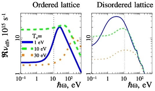
For and , (and hence the value of the density of absorbed power of laser radiation, which is proportional to ) is weakly dependent on , see Figure 2. For and , the value of is increasing with (the rate of the increase is proportional to ) for Umklapp processes in an ordered ion lattice, see [13]). For and , the value of is decreasing with , see Figure 2. The rate of such a decrease is proportional to for the case of a disordered ion lattice [12] and to for the case of an ordered ion lattice [13]. One should note here that the contribution of interband transitions to the dielectric function should be taken into account for quantum energies exceeding the gap between the conductivity band and inner electron energy levels [17]. As described above, the respective theoretical approach can be elaborated on the basis of the nonequilibrium statistical operator method. Note also that in the case of a disordered ion lattice (individual electron–ion and electron–electron interactions), Expressions (30) and (31) for the correlation functions give rise to the Ziman–Evans formula [39,40] for the electric conductivity in the limit [12].
4. Conclusions
The NSO method allows one to describe consistently the dielectric function of WDM in a wide range of frequencies and plasma parameters. Different kinds of electron–ion interactions, in particular in systems with a disordered distribution of ions (individual electron–ion and electron–electron interactions) and systems with an ordered ion configuration, described as an ion lattice (with collective electron–phonon interactions and Umklapp processes), are successfully treated using this method.
A main peculiarity of the absorption of irradiated laser energy in the case of an ordered ion lattice, owing to collective electron–phonon interactions and Umklapp processes, is a much stronger () decrease of the real part of the effective collision frequency at electron temperatures exceeding the Fermi temperature, if compared to the case of individual electron–ion and electron–electron interactions (where for ). An essential feature of the electron–phonon interaction and the Umklapp process is that they show, as a function of the electron temperature, a clear peak structure of the absorption coefficient and of the real part of the effective collision frequency at . In addition, in both cases of ordered and disordered ion lattices, the real part of the effective collision frequency as a function of the photon energy shows a peak structure: is nearly independent of for and , but is rising with ( for the case of ordered ion lattice) for , and is decreasing with ( for the case of ordered ion lattice and for the case of disordered ion lattice) for and .
The NSO method can be also applied for the description of interband contributions to the dielectric function, which are essential for photon energies exceeding the energy gaps between the conduction band and electron bands corresponding to excited electron energy levels. The relation to DFT calculation [17], which provides us with ab initio calculations of optimal single-electron states and replaces the approximation for the electron–ion potential used in our calculations, is of high interest. In addition, our approach allows one to take into account the contribution of electron–electron collisions to the dielectric function, which is not possible in mean-field approaches such as DFT. More detailed investigations of this case, as well as the calculation of the imaginary part of the effective collision frequency for the case of an ordered ion lattice with electron–phonon interactions and Umklapp processes, will be the subject of our future work.
Author Contributions
H.R. and G.R. have been working on the general concepts of the approach. M.V. has conducted the particular derivations and calculations.
Funding
The work of M.V. was partly supported by the Presidium of the RAS program “Thermo-physics of High Energy Density“, No I.13P. H.R. and G.R. acknowledge support by the DFG (German research foundation) via RE 975/4-1 and RO 905/32-1, respectively. G.R. acknowledges support from the MEPhI Academic Excellence Program under contract number 02.a03.21.0005.
Acknowledgments
We are greatfull to N.E. Andreev for valuable comments.
Conflicts of Interest
The authors declare no conflict of interest.
References
Zubarev, D.N. Relaxation and Hydrodynamic Processes, V 2. Dokl. Akad. Nauk SSSR Russ.1961, 140, 92. [Google Scholar]
Zubarev, D.N. Nonequilibrium Statistical Thermodynamics [in Russian: Neravnovesnaya Statistitsheskaya Termodinamika, Moscow, Nauka, 1971]; Plenum Press: New York, NY, USA, 1974. [Google Scholar]
Zubarev, D.N.; Morozov, V.; Röpke, G. Statistical Mechanics of Nonequilibrium Processes, V 1; Akademie Verlag/Wiley: Berlin, Germany, 1997. [Google Scholar]
Zubarev, D.N.; Morozov, V.; Röpke, G. Relaxation and Hydrodynamic Processes, V 2; Akademie Verlag/Wiley: Berlin, Germany, 1997. [Google Scholar]
Röpke, G. Electrical Conductivity of Charged Particle Systems and Zubarev’s Nonequilibrium Statistical Operator Method. Theor. Math. Phys.2018, 194, 74–104. [Google Scholar] [CrossRef]
Redmer, R. Physical properties of dense, low-temperature plasmas. Phys. Rep.1997, 282, 35–157. [Google Scholar] [CrossRef]
Reinholz, H. Dielectric and optical properties of dense plasmas. Ann. Phys. Fr.2005, 30, 1–187. [Google Scholar] [CrossRef]
Reinholz, H.; Röpke, G. Dielectric function beyond the random-phase approximation: Kinetic theory versus linear response theory. Phys. Rev. E2012, 85, 036401. [Google Scholar] [CrossRef]
Veysman, M.E.; Agranat, M.B.; Andreev, N.E.; Ashitkov, S.I.; Fortov, V.E.; Khishchenko, K.V.; Kostenko, O.F.; Levashov, P.R.; Ovchinnikov, A.V.; Sitnikov, D.S. Femtosecond optical diagnostics and hydrodynamic simulation of Ag plasma created by laser irradiation of a solid target. J. Phys. B At. Mol. Opt. Phys.2008, 41, 125704. [Google Scholar] [CrossRef]
Veysman, M.E.; Andreev, N.E. Semi-empirical model for permittivity of warm dense matter. J. Phys. Conf. Ser.2015, 653, 012004. [Google Scholar] [CrossRef]
Veysman, M.; Röpke, G.; Winkel, M.; Reinholz, H. Optical conductivity of warm dense matter within a wide frequency range using quantum statistical and kinetic approaches. Phys. Rev. E2016, 94, 013203. [Google Scholar] [CrossRef]
Veysman, M.; Röpke, G.; Reinholz, H. Analytical expression for high-frequency dielectric function of metals at moderate temperatures. J. Phys. Conf. Ser.2018, 946, 012012. [Google Scholar] [CrossRef]
Veysman, M.; Röpke, G.; Reinholz, H. High frequency dielectric function of metals taking into account Umklapp processes. J. Phys. Conf. Ser.2019, 1147, 012071. [Google Scholar] [CrossRef]
Kubo, R. Statistical-Mechanical Theory of Irreversible Processes. I. General Theory and Simple Applications to Magnetic and Conduction Problems. J. Phys. Soc. Jpn.1957, 12, 570–586. [Google Scholar] [CrossRef]
Röpke, G. Quantum-statistical approach to the electrical conductivity of dense, high-temperature plasmas. Phys. Rev. A1988, 38, 3001–3016. [Google Scholar] [CrossRef]
Reinholz, H.; Redmer, R.; Röpke, G.; Wierling, A. Long-wavelength limit of the dynamical local-field factor and dynamical conductivity of a two-component plasma. Phys. Rev. E2000, 62, 5648. [Google Scholar] [CrossRef]
Karakhtanov, V.S.; Redmer, R.; Reinholz, H.; Ropke, G. The Influence of Dynamical Screening on the Transport Properties of Dense Plasmas. Contrib. Plasma Phys.2013, 53, 639–652. [Google Scholar] [CrossRef]
Gericke, D.O.; Vorberger, J.; Wünsch, K.; Gregori, G. Screening of ionic cores in partially ionized plasmas within linear response. Phys. Rev. E2010, 81, 065401. [Google Scholar] [CrossRef]
Röpke, G.; Redmer, R. Electrical conductivity of nondegenerate, fully ionized plasmas. Phys. Rev. A1989, 39, 907–910. [Google Scholar] [CrossRef]
Ashcroft, N.; Stroud, D. Theory of the thermodynamics of simple liquid metals. Solid State Phys.1978, 33, 1–81. [Google Scholar]
Thakor, P.; Sonvane, Y.; Jani, A. Structural properties of some liquid transition metals. Phys. Chem. Liq.2011, 49, 530–549. [Google Scholar] [CrossRef]
Bretonnet, J.L.; Derouiche, A. Analytic form for the one-component plasma structure factor. Phys. Rev. B1988, 38, 9255–9256. [Google Scholar] [CrossRef]
Skupsky, S. “Coulomb logarithm” for inverse-bremsstrahlung laser absorption. Phys. Rev. A1987, 36, 5701–5712. [Google Scholar] [CrossRef]
Mahan, G.D. Many Particle Physics, 3rd ed.; Plenum: New York, NY, USA, 2000. [Google Scholar]
Hubbard, J. Electron correlations in narrow energy bands. Proc. R. Soc. Lond. Ser. A1963, 276, 238–257. [Google Scholar]
Christoph, V.; Röpke, G. Theory of Inverse Linear Response Coefficients. Phys. Status Solidi B1985, 131, 11–42. [Google Scholar] [CrossRef]
Povarnitsyn, M.E.; Andreev, N.E.; Apfelbaum, E.M.; Itina, T.E.; Khishchenko, K.V.; Kostenko, O.F.; Levashov, P.R.; Veysman, M.E. A wide-range model for simulation of pump-probe experiments with metals. Appl. Surf. Sci.2012, 258, 9480–9483. [Google Scholar] [CrossRef]
Agranat, M.; Andreev, N.; Ashitkov, S.; Veysman, M.; Levashov, P.; Ovchinnikov, A.; Sitnikov, D.; Fortov, V.; Khishchenko, K. Determination of the transport and optical properties of a nonideal solid-density plasma produced by femtosecond laser pulses. JETP Lett.2007, 85, 271–276. [Google Scholar] [CrossRef]
Huttner, B. A new method for the determination of the optical mass of electrons in metals. J. Phys. Condens. Matter1996, 8, 11041. [Google Scholar] [CrossRef]
Maksimov, E.G.; Savrasov, D.Y.; Savrasov, S.Y. The electron–phonon interaction and the physical properties of metals. Usp. Fiz. Nauk1997, 167, 353–376. [Google Scholar] [CrossRef]
Povarnitsyn, M.E.; Andreev, N.E. A wide-range model for simulation of aluminum plasma produced by femtosecond laser pulses. J. Phys. Conf. Ser.2016, 774, 012105. [Google Scholar] [CrossRef]
Cauble, R.; Rozmus, W. Two-temperature frequency-dependent electrical resistivity in solid density plasmas produced by ultrashort laser pulses. Phys. Rev. E1995, 52, 2974–2981. [Google Scholar] [CrossRef]
Ziman, J.M. A Theory of Electrical Properties of Liquid Metals. The Monovalent Metals. Philos. Mag.1961, 6, 1013–1034. [Google Scholar] [CrossRef]
Evans, R. The resistivity and thermopower of liquid mercury and its alloys. J. Phys. C Solid State Phys.1970, 3, S137–S152. [Google Scholar] [CrossRef]
Figure 1.
Absorption coefficient (first row) as well as real (second row) and imaginary (third row) parts of the complex collision frequency of electrons (46), as a function of the electron temperature , for a solid-density aluminum plasma ( g/cm) and laser radiation of different wavelengths (left column: 80 nm; center: 0.4 m; right: 10 m). Curves are shown for different ion temperatures (see legend), calculated for the case of an ordered lattice by Models (46), (51), and (52) (with an account of electron–phonon interactions and Umklapp processes, labeled by “e-ph”), as well as for the case of a disordered lattice (electron–ion and electron–electron interactions, labeled by “e-i”). Curves with the markers “*” and “⋄” are according to the models cited in the text (see legend).
Figure 2.
The absorption coefficient and the real part of the complex collision frequency of electrons (46) in a solid-density aluminum plasma are shown as a function of the laser frequency for ion temperatures eV and different electron temperatures (see legend). Thick curves (left column) refer to the case of an ordered lattice with electron–phonon interactions and Umklapp processes, and thin curves (right column) refer to a disordered lattice with electron–ion and electron–electron interactions.
Veysman, M.; Röpke, G.; Reinholz, H.
Application of the Non-Equilibrium Statistical Operator Method to the Dynamical Conductivity of Metallic and Classical Plasmas. Particles2019, 2, 242-260.
https://doi.org/10.3390/particles2020017
AMA Style
Veysman M, Röpke G, Reinholz H.
Application of the Non-Equilibrium Statistical Operator Method to the Dynamical Conductivity of Metallic and Classical Plasmas. Particles. 2019; 2(2):242-260.
https://doi.org/10.3390/particles2020017
Chicago/Turabian Style
Veysman, Mikhail, Gerd Röpke, and Heidi Reinholz.
2019. "Application of the Non-Equilibrium Statistical Operator Method to the Dynamical Conductivity of Metallic and Classical Plasmas" Particles 2, no. 2: 242-260.
https://doi.org/10.3390/particles2020017
APA Style
Veysman, M., Röpke, G., & Reinholz, H.
(2019). Application of the Non-Equilibrium Statistical Operator Method to the Dynamical Conductivity of Metallic and Classical Plasmas. Particles, 2(2), 242-260.
https://doi.org/10.3390/particles2020017
Article Metrics
No
No
Article Access Statistics
For more information on the journal statistics, click here.
Multiple requests from the same IP address are counted as one view.
Veysman, M.; Röpke, G.; Reinholz, H.
Application of the Non-Equilibrium Statistical Operator Method to the Dynamical Conductivity of Metallic and Classical Plasmas. Particles2019, 2, 242-260.
https://doi.org/10.3390/particles2020017
AMA Style
Veysman M, Röpke G, Reinholz H.
Application of the Non-Equilibrium Statistical Operator Method to the Dynamical Conductivity of Metallic and Classical Plasmas. Particles. 2019; 2(2):242-260.
https://doi.org/10.3390/particles2020017
Chicago/Turabian Style
Veysman, Mikhail, Gerd Röpke, and Heidi Reinholz.
2019. "Application of the Non-Equilibrium Statistical Operator Method to the Dynamical Conductivity of Metallic and Classical Plasmas" Particles 2, no. 2: 242-260.
https://doi.org/10.3390/particles2020017
APA Style
Veysman, M., Röpke, G., & Reinholz, H.
(2019). Application of the Non-Equilibrium Statistical Operator Method to the Dynamical Conductivity of Metallic and Classical Plasmas. Particles, 2(2), 242-260.
https://doi.org/10.3390/particles2020017


