Abstract
We present a novel numerical scheme to solve the QCD Boltzmann equation in the soft scattering approximation, for the quenched limit of QCD. Using this we can readily investigate the evolution of spatially homogeneous systems of gluons distributed isotropically in momentum space. We numerically confirm that for so-called “overpopulated” initial conditions, a (transient) Bose-Einstein condensate could emerge in a finite time. Going beyond existing results, we analyze the formation dynamics of this condensate. The scheme is extended to systems with cylindrically symmetric momentum distributions, in order to investigate the effects of anisotropy. In particular, we compare the rates at which isotropization and equilibration occur. We also compare our results from the soft scattering scheme to the relaxation time approximation.
1. Introduction
The study of quark-gluon plasma (QGP), the phase of strongly interacting matter formed in relativistic nuclear collisions and consisting of quasi-free quarks and gluons, is of increasing relevance in modern physics [1]. It represents a testing ground for the Standard Model, as well as for finite temperature field theory and possible grand unification theories. It is also of cosmological significance, as the early universe was dominated by this phase of matter.
Experiments at the Super Proton Synchrotron (SPS), Relativistic Heavy Ion Collider (RHIC) and Large Hadron Collider (LHC) allow us to probe the energy scales at which the QGP is produced. Inferring its properties and phenomenological behaviour is a central goal of the heavy ion programs at these facilities. The theoretical tools that have been developed to describe it are manifold, as the various stages of a heavy ion collision represent very different physical regimes that demand similarly diverse mathematical formalisms to describe (see Figure 1).
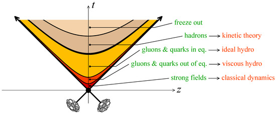
Figure 1.
The stages of a heavy ion collision (from [1]).
Prior to the collision, the nuclei are accelerated to near-light speed, with a Lorentz factor on the order of 100. They are therefore subject to strong Lorentz contraction along the beam axis. At these energies, the lifetime of gluons emitted from the valence quarks or other gluons is long enough to allow additional emissions of soft gluons from themselves. This process keeps increasing the number density of gluons until saturation occurs as recombination of gluons becomes non-negligible, forming the state of matter called the Color Glass Condensate (CGC) [2,3,4]. This regime of large gluon number can be approximated by classical dynamics.
In the first stage of a collision, a large number of gluons are liberated from the CGC. These gluons form a dense, off-equilibrium state called the glasma. Extensive hydrodynamic analyses of HIC indicate that as the medium expands, rapid thermalization occurs (characteristic time on the order of 1 fm) and a QGP in local equilibrium forms [5,6,7,8]. This rapid thermalization is indicative of strong interactions. As the medium continues to expand and decrease in temperature, it eventually drops below the deconfinement temperature and hadronization occurs.
Despite longstanding efforts and various approaches to describe the dynamics of heavy ion collisions (see e.g., [9,10]), the rapid equilibration of the QGP remains to be thoroughly understood. Another question that has received a lot of recent attention is the possible formation of a gluon condensate in heavy ion collisions [11,12]. We will address these two questions by adapting and numerically solving the QCD Boltzmann equation assuming the dominance of soft gluon exchange in binary collisions. In this framework we can describe the evolution of the QGP from the early pre-equilibrium stages through thermalization towards freeze-out.
2. The Boltzmann Transport Equation
The fundamental equation of kinetic theory is the Boltzmann transport equation. It is a non-linear integro-differential equation describing the evolution of a distribution function of particles, for our purposes a dilute gas of gluons “in a box”. (Quarks are omitted for conceptual simplicity and also motivated for systems which are gluon-dominated). For a spatially homogeneous system under the assumption that processes dominate, it can be written as
Here is the distribution function of particle i with 4-momentum . As shorthand, we write .
The transition amplitude of binary gluon scattering reads at tree level
where s, t and u are the familiar Mandelstam variables and g is related to the QCD coupling constant by .
For small scattering angles, and expression (2) simplifies to
which is to be regulated, e.g., by making the substitution
where is the screening mass.
While this equation is a challenge to solve, Boltzmann’s H-Theorem guarantees that regardless of the initial condition, the equilibrium distribution function will be a Bose-Jüttner function [13],
Here T, u and parameterize the temperature, collective flow velocity and chemical potential, respectively.
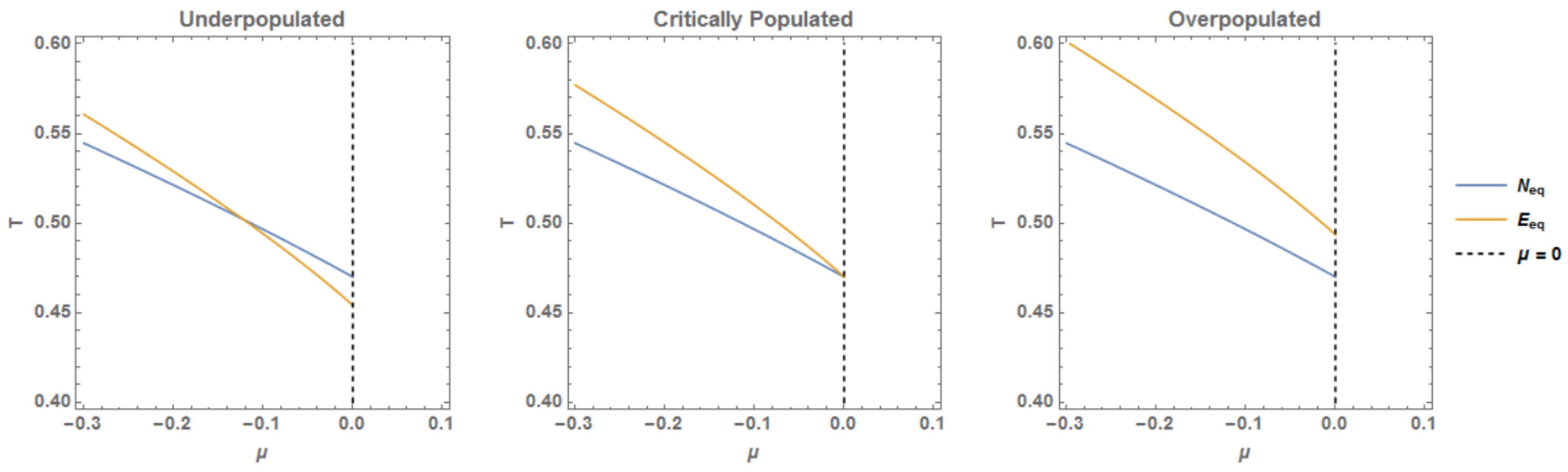
There is one caveat; there exist “overpopulated” initial distributions (see Figure 2) which contain more gluons than can be “accommodated” in a Bose-Jüttner distribution while maintaining particle number and energy conservation. It has been argued [11] that under the assumption of approximate gluon number conservation, a transient state close to equilibrium may form with a Bose-Einstein condensate.
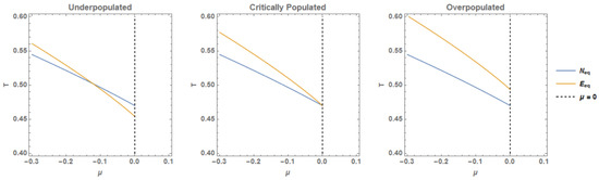
Figure 2.
Contours of constant particle number and energy density at equilibrium. The values of the equilibrium parameters T and are found where the lines intersect. In the critically populated case, the intersection occurs at the maximum possible value of . In the overpopulated case, no real solution for exists and a condensate is necessary to contain the excess particles.
3. The Fokker-Planck and Relaxation Time Approximations
Under the assumption that small-angle scattering dominates, the RHS of Equation (1) can be approximated as the divergence of a current in momentum space [11],
which is a Fokker-Planck type equation. Here the components of the current read
where
and we define , and denote the corresponding unit vectors by and .
In Equation (7), is the so-called Coulomb logarithm emerging for screened interactions with vector boson exchange, where and are cutoffs of the order of the equilibrium temperature T and the screening mass introduced in expression (4), respectively [11]. We take to be a constant of order 1 in our analysis.
It is convenient to rescale the time variable in Equation (6) as to eliminate the constant factor in Equation (7). The integral in (7) can then be performed (see Appendix A), yielding
where , and are functionals of the distribution function f.
It will be interesting to compare the Fokker-Planck approximation of the Boltzmann equation to the well-known Relaxation Time Approximation (RTA),
The RTA is easily solvable (and convergences to the same equilibrium distribution); however it lacks QCD-specific features and, as we will see, yields qualitatively different behavior to the Fokker-Planck approximation, which we argue is more physically motivated.
4. The Method of ’B-Lines’
We have developed a flux-conservative numerical scheme that allows us to readily solve the Boltzmann equation in the Fokker-Planck approximation, (6) + (9), which we call the method of ‘B-lines’. The name is given in analogy to splines, with the ’B’ referring to an efficient parameterization of the distribution function in terms of piecewise Bose functions. We have implemented it for distribution functions spherically and cylindrically symmetric in momentum space; here we will discuss the scheme for the simpler isotropic case.
For spherically symmetric distribution functions, we discretize the momentum grid into bins of width and construct a piecewise Bose interpolation of f,
The domain of is for and for .
A couple of points are in order. Firstly, it should be noted that this approach is equivalent to a linear interpolation of an expedient transformation of the distribution function, , i.e., . One of the reasons that we choose to make this transformation is that a piecewise linear interpolation directly in terms of f would not allow us to describe the formation of the Bose-Einstein condensate. Secondly, for equilibrium distribution functions approaching equilibrium our interpolation scheme becomes exact, which is a nice property. An equilibrium distribution in g-space of course is simply a straight line.
Physically, the correspond to local (in momentum space) inverse temperature parameters, and the correspond to the chemical potential. We determine them by sampling the distribution function at the gridpoints,
Here is small relative to but non-zero in order to avoid singularities at the origin.
Having established the details of the initial interpolation, we now consider the process by which we evolve the distribution function in time. We separate our cells on the p-axis at the momenta
such that cell 0 is , cell M is and intermediate cells with index are . These cell boundaries are “staggered” with respect to the grid used for the interpolation, with the distribution function in each cell being interpolated by two B-lines. This is because as we will see shortly, the first derivative of our interpolation of the distribution function is required to be continuous at our cell boundaries, which is not in general the case at B-line boundaries.
From the B-lines we can easily calculate the particle number (per volume) in each cell,
These integrals are combinations of polylogarithm functions depending on the B-line parameters . For convenience we have set the gluon degeneracy to 1; can be reinstated as needed.
Now, recall that the Fokker-Planck equation (6) can be written as a continuity equation (conserving both particle number and energy). Thus the rate of change of particle number in cell i,
is given by , the net radial flux into cell i, where
For the zeroth cell, the flux at is zero by definition. Similarly, the last cell’s rightmost boundary is at infinity, with zero flux through it.
We thus arrive at the following non-linear system of ODEs,
Note that the integrals and ( vanishes in the spherically symmetric case), which determine the flux (16) depend non-linearly on all of the and must be updated at each time step. We can readily solve these ODEs using the forward Euler method. Having updated the particle number in each cell, it is straightforward to find the evolved set of B-line parameters.
One advantage of the modified scheme is that it allows us to compute the number of particles in the condensate. Analysis shows that the flux into the zeroth cell becomes non-zero after finite time for overpopulated systems approaching the equilibrium Bose-Einstein distribution. Note that this flux remains well-defined as we take the limit . For large t, the flux becomes proportional to , which vanishes for an equilibrium distribution. The particle number in cell 0 has a “regular” contribution, which vanishes for , as well as the condensate contribution.
5. Results
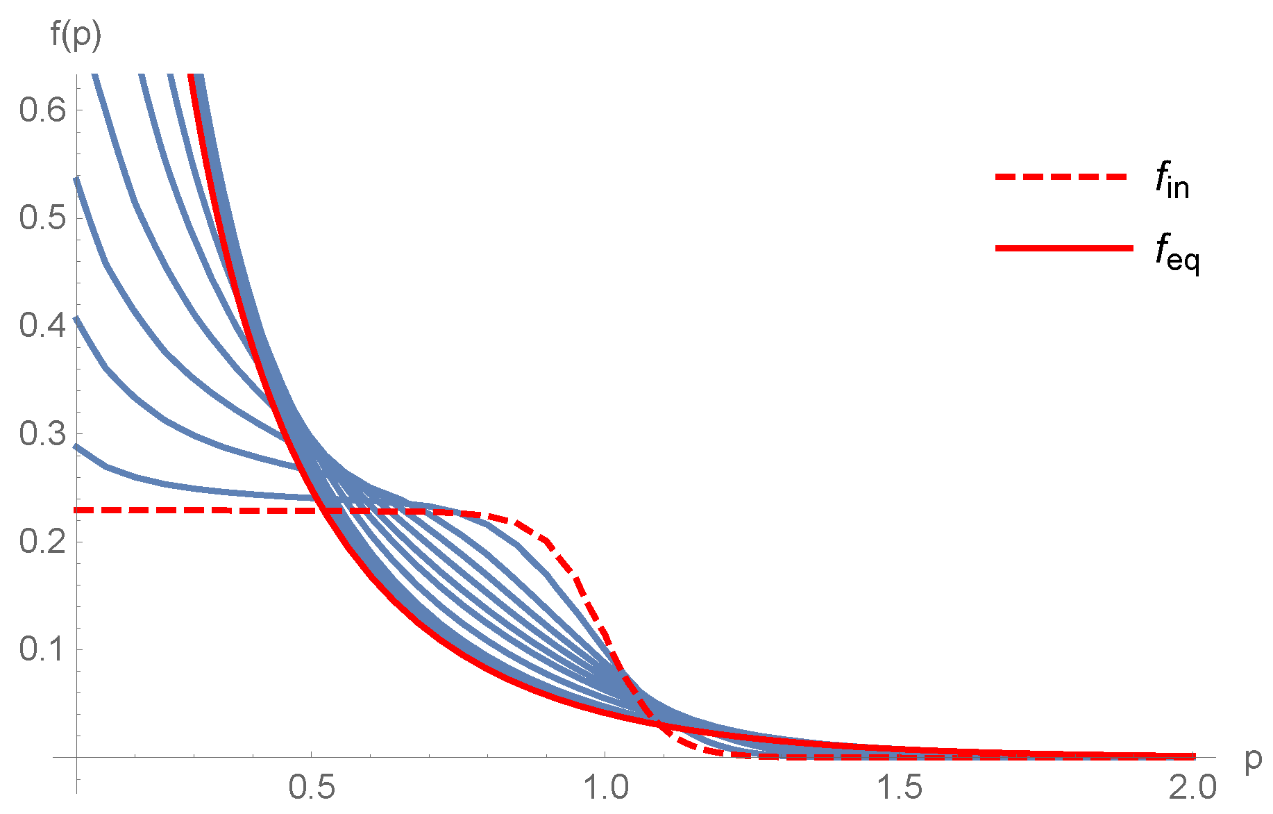
Figure 3, Figure 4, Figure 5 and Figure 6 show the evolution in the special case of spherically symmetric, CGC-inspired initial conditions of the form
where and C are constants and Q sets the overall momentum scale. For these figures, we have chosen and (and ), which is a moderately overpopulated initial condition where some of the particles asymptotically condense. We point out the qualitative difference between the Fokker-Planck and Relaxation Time Approximations; in the latter the condensate begins to form immediately, whereas the Fokker-Planck scheme exhibits a characteristic “lag”. The onset time is fairly short, assuming , and GeV we find fm/c.
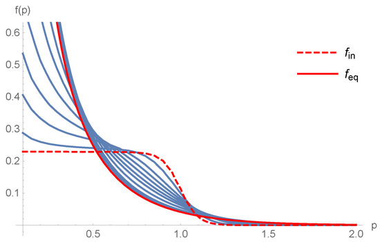
Figure 3.
Evolution of the initial condition according to the Fokker-Planck scheme. The intermediate distribution functions shown are for times .

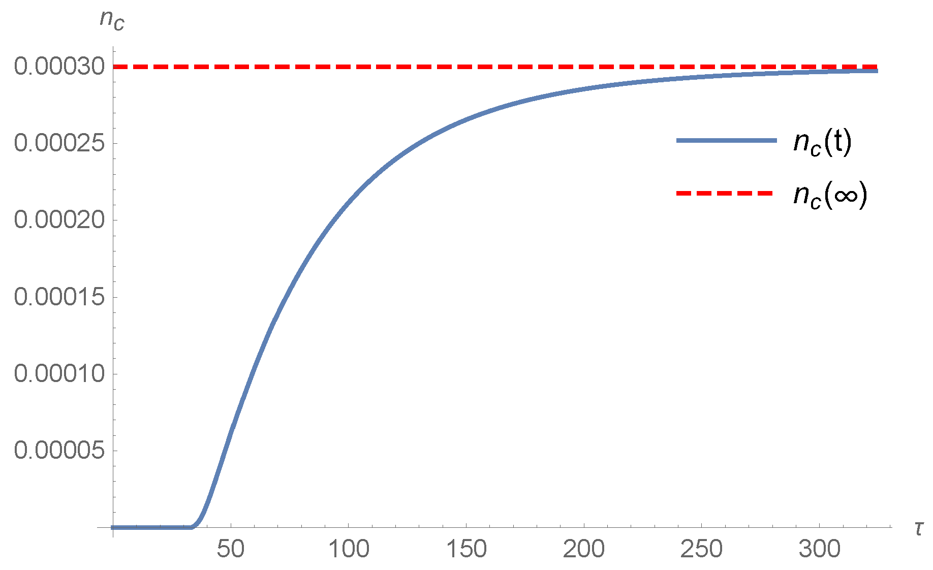
Figure 4.
Corresponding evolution of the condensate for the system in Figure 3.
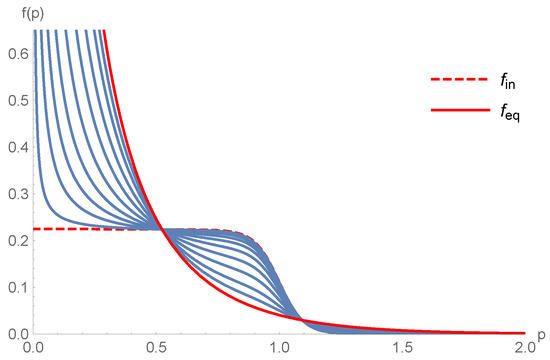
Figure 5.
Evolution of the initial condition using the Relaxation Time Approximation. The relaxation time parameter is taken to be 40 in order to match the Fokker-Planck timescale; the intermediate distribution functions shown are for times .
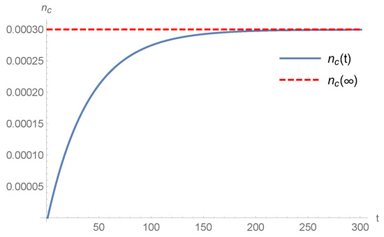
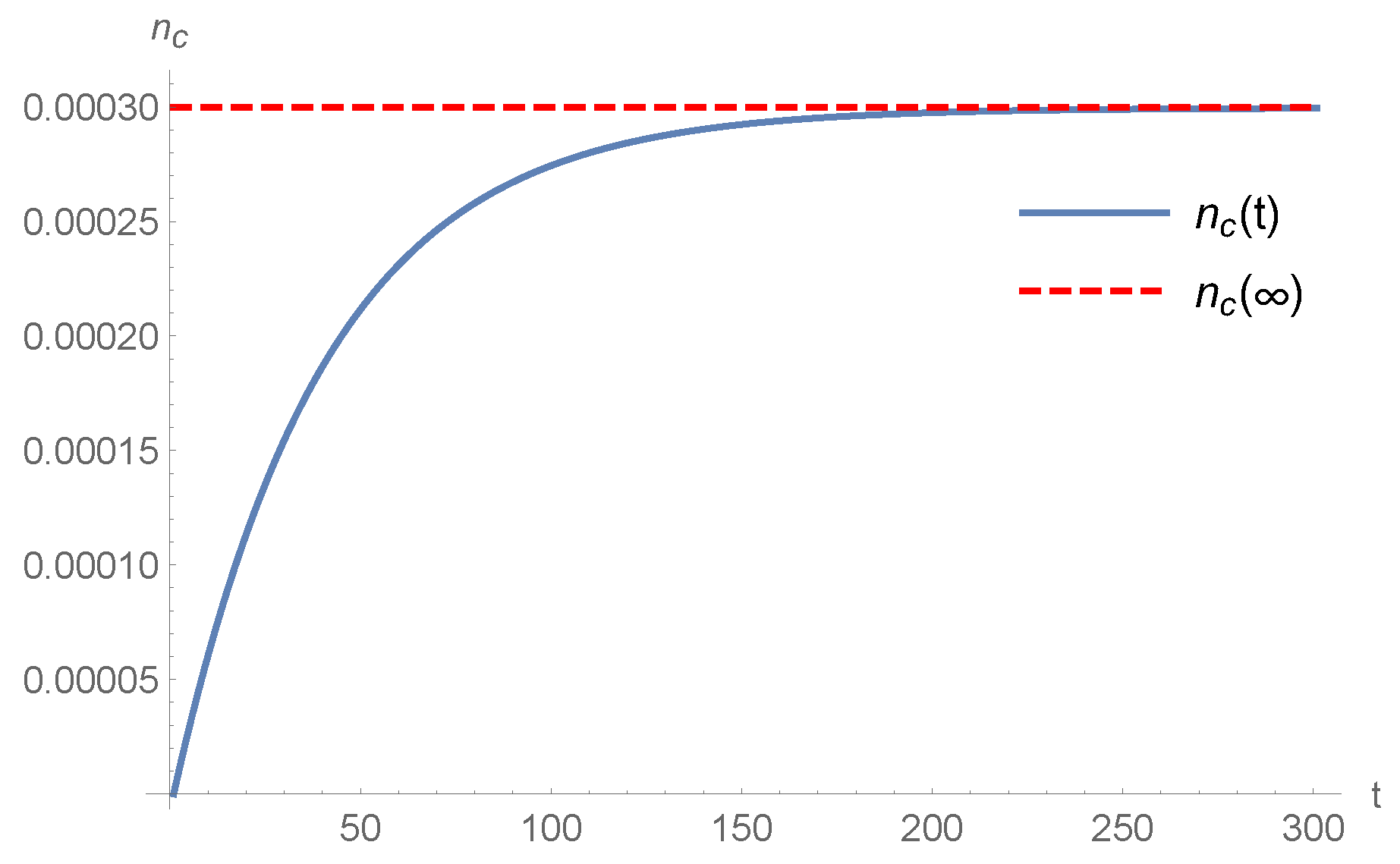
Figure 6.
Corresponding evolution of the condensate for the system in Figure 5.
Generalizing from spherically symmetric to cylindrically symmetric initial conditions, we are able to explore the effects on anisotropy on the evolution of the distribution function. It is important to differentiate between isotropic distribution functions just boosted out of their rest frame and distribution functions that are “genuinely” anisotropic, i.e., even in their rest frame.
“Genuinely” anisotropic distributions are often parameterized in the form [14,15]
where specifies the anisotropy. Similarly, we consider as a generalization of (18) initial conditions of the form
where , b is a boost parameter and the numerator is a normalization that is convenient with regard to the particle number density.
We extract the equilibration time by studying the entropy, evaluated towards final equilibrium. In particular we would like to compare it to the time taken for the initially anisotropic distribution function to isotropize. To this end, as a measure of the anisotropy of a distribution function, we define the “anisotropy parameter”
where is the energy-momentum tensor in the local rest frame. In the rest frame, for a cylindrically symmetric distribution function with some anisotropy, is the transverse pressure of the fluid, while is the longitudinal pressure. For an isotropic distribution they are equal; thus the ratio must also approach 1 as the system isotropizes.
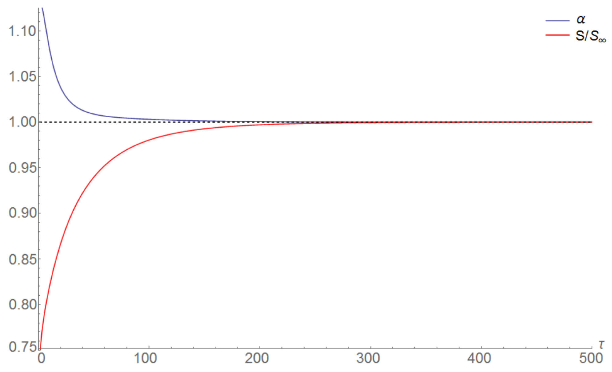
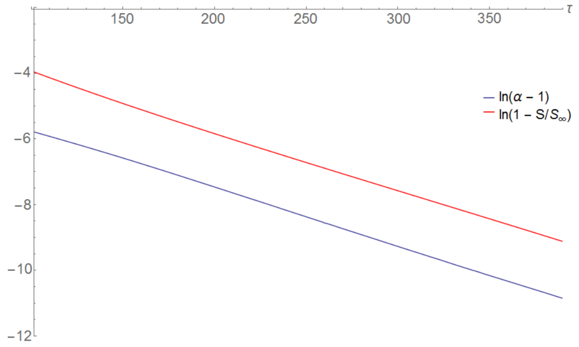
In Figure 7 we plot the evolution of the normalized entropy and anisotropy parameters associated with an initial condition of form (20), with parameters and . Figure 8 shows a log plot of this evolution.
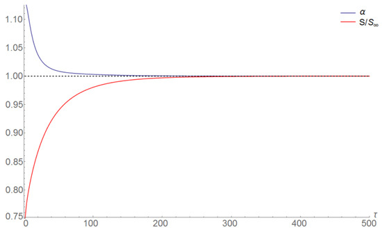
Figure 7.
.Evolution of the normalized entropy and anisotropy parameters.
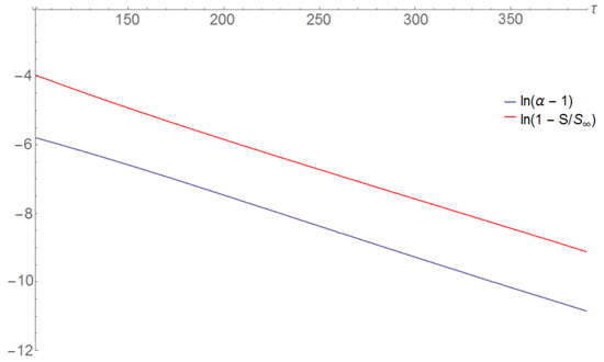
Figure 8.
Linearized evolution of the normalized entropy and anisotropy parameters.
From a fit, the gradients of the lines in Figure 7 are identical within the uncertainties, which corroborates that the rates of isotropization and equilibration are strongly correlated.
6. Discussion
In summary, we have developed an efficient numerical scheme to solve the relativistic Boltzmann equation for gluons in the small-scattering approximation under the assumption of spherically/cylindrically symmetric initial conditions and spatial homogeneity. Among our findings, we have reproduced results from [11] regarding the formation of a transient Bose-Einstein condensate state for overpopulated, spherically symmetric initial conditions. We have investigated the rate at which an anisotropic distribution function becomes isotropic and compared it to the rate of thermalization. Further, we have compared these results to the relaxation-time approximation to the Boltzmann equation.
Possible directions for future work might include investigating the timescale of hydrodynamization (i.e., the time at which hydrodynamics becomes applicable). Following [16], it would be interesting to explore the relation between Bose-Einstein condensation and Kolmogorov turbulence in the relativistic case. Another follow-up would be to study the non-equilibrium attractor described by [17] for the relaxation-time approximation, and see if a similar phenomenon can be observed in the Fokker-Planck approximation.
Scope for further extension of our scheme exists, and such an extension is planned. In particular, it is desirable to extend the scheme to remove the assumption of spatial homogeneity and describe systems without symmetry assumptions in which the above scheme would essentially represent a single spatial cell. A challenge is the fact that the computational complexity scales geometrically with each additional degree of freedom - the so-called “curse of dimensionality”. (Boltzmann equation solvers as well as hydro-codes typically rely on assumptions of symmetry, and for good reason).
Author Contributions
This work is based on the M.Sc. thesis written by B.H. and supervised by A.P.
Funding
This research was funded by NiTheP.
Acknowledgments
The authors are grateful for conversations and coding assistance provided by Nicole Moodley, Will Grunow and Greg Jackson.
Conflicts of Interest
The authors declare no conflict of interest.
Appendix A. Derivation of the Current
Here we present a derivation of the Fokker-Planck current given in Equation (9). Recall expression (7) for the current, where the constant prefactor is absorbed into ,
These two integrals correspond to a vector quantity
and a tensor quantity
each being a functional of the distribution function f. The current (A1) is defined for a specific momentum . For this we then integrate over all possible values of . We can represent the tensor (8) as a matrix,
Thus we find for the components of the first integral in (A1),
Note that since the distribution function vanishes for large momenta. Thus only terms of survive. Integrating by parts we have
with corresponding expressions for and .
Altogether, the non-vanishing terms of are
Similarly
Defining
we can simply write
Now consider the tensor term (A3). Expanding we have
We can tidy this expression by defining
and writing . As it is no longer necessary to differentiate between and , we drop the subscript. Then
and similarly
and
We can write down a vector expression for by inspection as .
Altogether we have the complete expression for the current,
References
- Gelis, F. The early stages of a high energy heavy ion collision. J. Phys. Conf. Ser. 2012, 381, 012021. [Google Scholar] [CrossRef]
- McLerran, L.; Venugopalan, R. Computing Quark and Gluon Distribution Functions for Very Large Nuclei. Phys. Rev. D 1994, 49, 2233–2241. [Google Scholar] [CrossRef]
- Weigert, H. Evolution at small x_bj: The Color Glass Condensate. Prog. Part. Nucl. Phys. 2005, 55, 461–565. [Google Scholar] [CrossRef]
- Gelis, F. Initial State and Thermalization in the Color Glass Condensate Framework. In Quark–Gluon Plasma 5; World Scientific: Singapore, 2016; pp. 67–129. ISBN 9789814663700. [Google Scholar]
- Heinz, U.W.; Kolb, P.F. Early thermalization at RHIC. Nucl. Phys. A 2002, 702, 269–280. [Google Scholar] [CrossRef]
- Romatschke, P.; Romatschke, U. Viscosity Information from Relativistic Nuclear Collisions: How Perfect is the Fluid Observed at RHIC? Phys. Rev. Lett. 2007, 99, 172301. [Google Scholar] [CrossRef] [PubMed]
- Ollitrault, J.-Y. Relativistic hydrodynamics for heavy-ion collisions. Eur. J. Phys. 2008, 29, 275–302. [Google Scholar] [CrossRef]
- Romatschke, P.; Romatschke, U. Relativistic Fluid Dynamics In and Out of Equilibrium—Ten Years of Progress in Theory and Numerical Simulations of Nuclear Collisions. arXiv 2017, arXiv:1712.05815. [Google Scholar]
- Biro, T.S.; van Doorn, E.; Mueller, B.; Thoma, M.H.; Wang, X.N. Parton Equilibration in Relativistic Heavy Ion Collisions. Phys. Rev. C 1993, 48, 1275–1284. [Google Scholar] [CrossRef]
- van der Schee, W. Equilibration and hydrodynamics at strong and weak coupling. Nucl. Phys. A 2017, 967, 74–80. [Google Scholar] [CrossRef]
- Blaizot, J.-P.; Liao, J.; McLerran, L. Gluon transport equation in the small angle approximation and the onset of Bose–Einstein condensation. Nucl. Phys. A 2013, 920, 58–77. [Google Scholar] [CrossRef]
- Blaizot, J.-P.; Liao, J.; Mehtar-Tani, Y. The thermalization of soft modes in non-expanding isotropic quark gluon plasmas. Nucl. Phys. A 2017, 961, 37–67. [Google Scholar] [CrossRef]
- Giulini, D. Luciano Rezzolla and Olindo Zanotti: Relativistic Hydrodynamics; Oxford University Press: Oxford, UK, 2013; 752p, ISBN 978-0-19-852890-6. [Google Scholar]
- Romatschke, P.; Strickland, M. Collective Modes of an Anisotropic Quark-Gluon Plasma. Phys. Rev. D 2003, 68, 036004. [Google Scholar] [CrossRef]
- Romatschke, P.; Strickland, M. Collective modes of an Anisotropic Quark-Gluon Plasma II. Phys. Rev. D 2004, 70, 116006. [Google Scholar] [CrossRef]
- Semikoz, D.V.; Tkachev, I.I. Condensation of bosons in kinetic regime. Phys. Rev. D 1997, 55, 489–502. [Google Scholar] [CrossRef]
- Strickland, M. The non-equilibrium attractor for kinetic theory in relaxation time approximation. J. High Energy Phys. 2018, 2018, 128. [Google Scholar] [CrossRef]


© 2019 by the authors. Licensee MDPI, Basel, Switzerland. This article is an open access article distributed under the terms and conditions of the Creative Commons Attribution (CC BY) license (http://creativecommons.org/licenses/by/4.0/).