Reworking Zubarev’s Approach to Nonequilibrium Quantum Statistical Mechanics

Abstract

In this work, the nonequilibrium density operator approach introduced by Zubarev more than 50 years ago to describe quantum systems at a local thermodynamic equilibrium is revisited. This method, which was used to obtain the first “Kubo” formula of shear viscosity, is especially suitable to describe quantum effects in fluids. This feature makes it a viable tool to describe the physics of Quark–Gluon Plasma in relativistic nuclear collisions.

1. Introduction

One of the authors (F.B.) would like to start this paper with a personal recollection. I first ran across Zubarev’s papers when I was studying the derivation by A. Hosoya et al. [1] of the shear viscosity in quantum-field theory, a result widely known as “Kubo formula”, like many of the same sort. This derivation was overtly based on Zubarev’s method of nonequilibrium density (or statistical) operator, and I surmised that this method must have been a very important and renowned tool in quantum statistical mechanics. In fact, surprisingly, it could hardly be found in textbooks and in the recent literature, and I did not quite understand why the founding method of such an important formula was that overlooked. After some more self-education, I realized that, perhaps part of the problem was that Zubarev himself did not put the right emphasis on the crucial feature that his proposed operator should possess: to be stationary, hence well-suited to be used in relativistic quantum-field theory as a density operator in the Heisenberg representation. A nonequilibrium stationary density operator sounds somewhat contradictory, but this is not the case if we deal with a system that, at some time, is known to be in local thermodynamic equilibrium, as we see in more detail in Section 3.

In this work, we would like to not just summarize Zubarev’s method [2,3,4], but also to make a critical appraisal and to provide a reformulation thereof that highlights the important features of this approach in a hopefully clear fashion. I also hope that this work could do justice to Zubarev and his remarkable achievement.

Notation

In this paper we use natural units, with $\hslash =c=K=1$.

The Minkowskian metric tensor is $\mathrm{diag}(1,-1,-1,-1)$; for the Levi-Civita symbol, we use convention ${ϵ}^{0123}=1$.

Operators in the Hilbert space are denoted by a large upper hat, e.g., $\widehat{T}$, while unit vectors with a small upper hat, e.g., $\widehat{v}$. Scalar products and contractions are sometimes denoted with a dot, e.g., $A_{\mu }{B}^{\mu }=A·B$.

2. Local Thermodynamic Equilibrium

Zubarev formalism can be used in nonrelativistic as well as in relativistic quantum statistical mechanics. We can then start from the latter, more general case, which is applicable to relativistic fluids out of equilibrium [5]. The relativistic version of the nonequilibrium density operator was first put forward by Zubarev himself and his collaborators in 1979 [6], and later reworked by Van Weert in Reference [7].

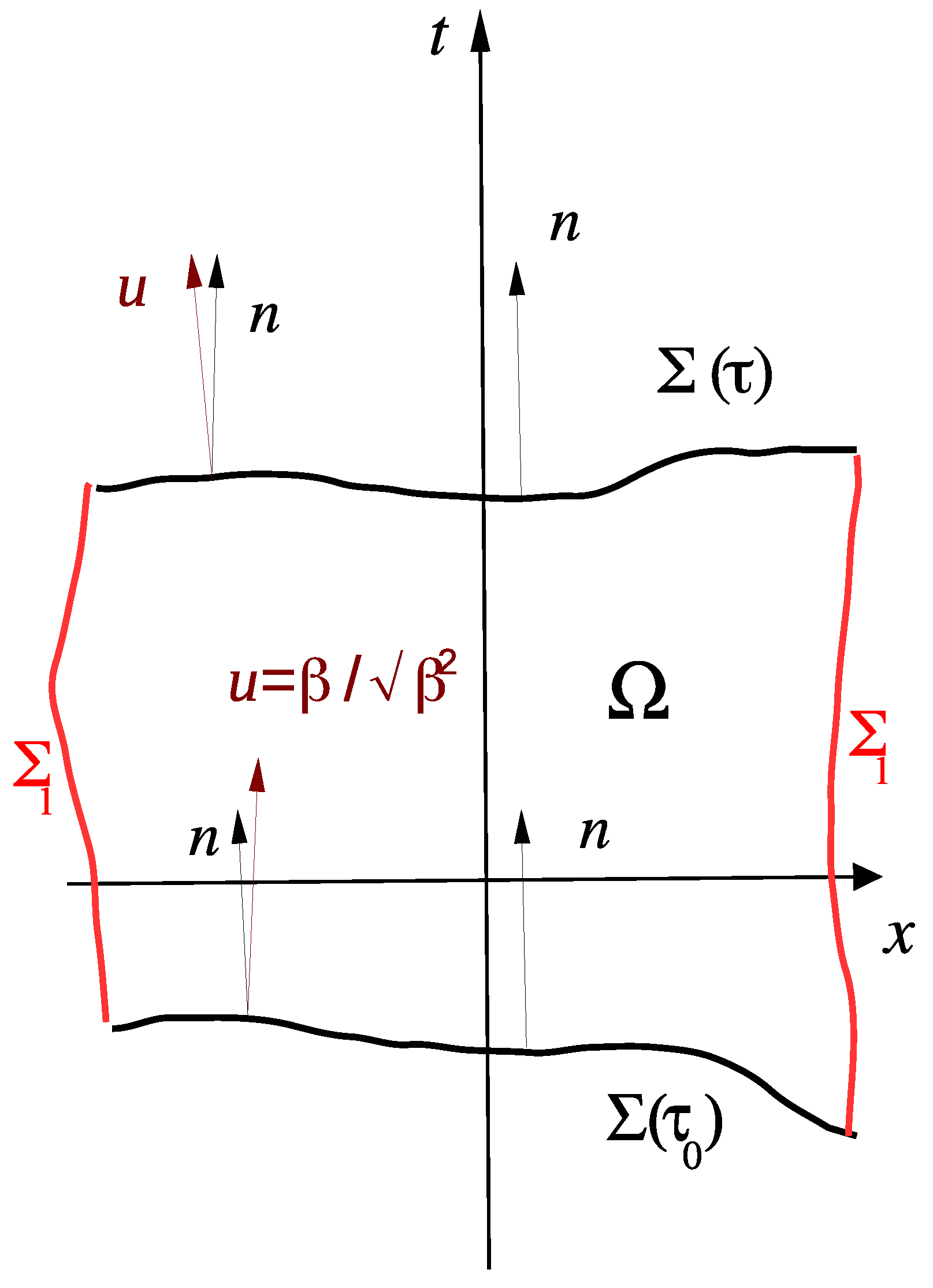
The starting point is the definition of the local equilibrium density operator. In relativity, this notion needs the specification of a one-parameter family of 3D spacelike hypersurfaces $\Sigma \left(\tau \right)$ (see Figure 1), also known as foliation of spacetime [6,7,8,9]. “Time” $\tau$ does not necessarily coincide with the proper time marked by comoving clocks. Local equilibrium density operator ${\widehat{\rho }}_{\mathrm{LE}}$ is obtained by maximizing the total entropy:

$$S=-\mathrm{tr}(\widehat{\rho }log\left(\widehat{\rho }\right))$$

(1)

with constrained values of energy–momentum and charge density, which should be equal to the actual values. In a covariant formulation, these densities are obtained by projecting the mean values of the stress–energy tensor and current onto the normalized vector perpendicular to $\Sigma$:

$$n_{\mu }\mathrm{tr}\left(\widehat{\rho }{\widehat{T}}^{\mu \nu }\right)=n_{\mu }{T}^{\mu \nu },n_{\mu }\mathrm{tr}\left(\widehat{\rho }{\widehat{j}}^{\mu }\right)=n_{\mu }{j}^{\mu }.$$

(2)

where $T^{\mu \nu }$ and $j^{\mu }$ are the true values of the stress–energy and current fields. The operators in Equation (2) are in the Heisenberg representation. In addition to the energy, momentum, and charge densities, one should include the angular momentum density, but if the stress–energy tensor is the Belinfante [10], this further constraint is redundant and can be disregarded.

The resulting operator is the Local Equilibrium Density Operator (LEDO):

$${\widehat{\rho }}_{\mathrm{LE}}={\displaystyle \frac{1}{Z_{\mathrm{LE}}}}exp\left[-{\int }_{\Sigma \left(\tau \right)}\mathrm{d}\Sigma n_{\mu }\left({\widehat{T}}^{\mu \nu }\left(x\right){\beta }_{\nu }\left(x\right)-\zeta \left(x\right){\widehat{j}}^{\mu }\left(x\right)\right)\right]$$

(3)

where $\beta$ and $\zeta$ are the relevant Lagrange multiplier functions for this problem, whose meaning is the four-temperature vector and the ratio between local chemical potential and temperature, respectively [8], $\mathrm{d}\Sigma$ is the measure of the hypersurface induced by the Minkowskian metric, and fields $\beta$ and $\zeta$ are the solution of Constraints (2) with $\widehat{\rho }={\widehat{\rho }}_{\mathrm{LE}}$, namely:

$$n_{\mu }\mathrm{tr}\left({\widehat{\rho }}_{\mathrm{LE}}{\widehat{T}}^{\mu \nu }\right)=n_{\mu }{T}_{\mathrm{LE}}^{\mu \nu }[\beta ,\zeta ,n]=n_{\mu }{T}^{\mu \nu },n_{\mu }\mathrm{tr}\left({\widehat{\rho }}_{\mathrm{LE}}{\widehat{j}}^{\mu }\right)=n_{\mu }{j}_{\mathrm{LE}}^{\mu }[\beta ,\zeta ,n]=n_{\mu }{j}^{\mu }.$$

(4)

These equations indeed define a vector field $\beta$, which, in turn, can be used as a hydrodynamic frame, $\beta$ [8] or thermodynamic frame [11], by identifying the four-velocity with

$$u=\frac{\beta }{\sqrt{{\beta }^2}}=T\beta ,$$

(5)

which somehow inverts the usual definition.

It is important to stress that the LEDO in Equation (3) is not stationary because operators are generally time-dependent. The sufficient condition for stationarity is that $\beta$ is a killing vector field, and $\zeta$ a constant; in this case, the LEDO becomes the general global thermodynamic equilibrium operator [12].

3. Nonequilibrium Density Operator Revisited

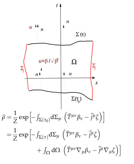
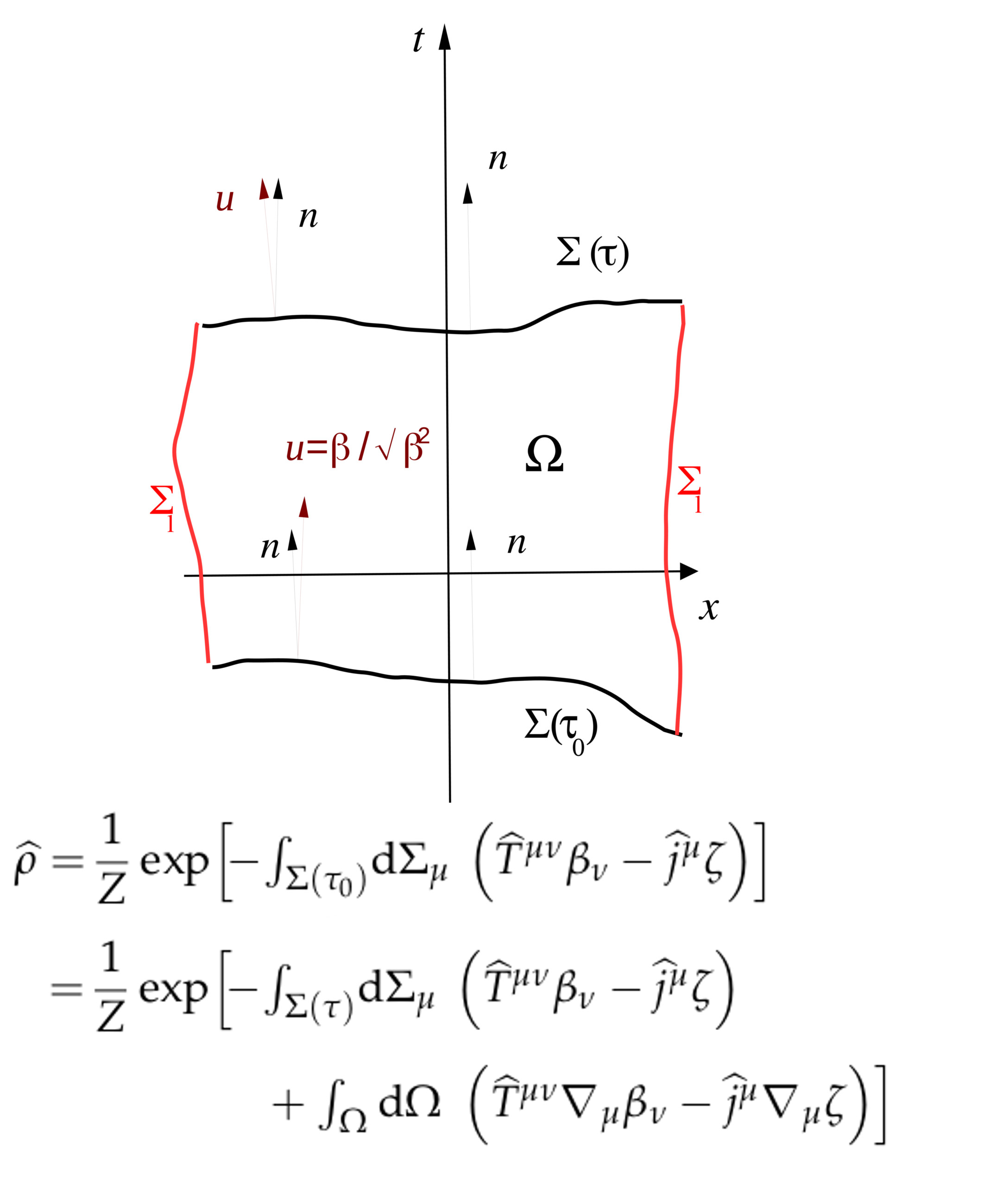
The true density operator in the Heisenberg representation must be stationary by definition, whereas the LEDO is not. The solution of how to work it out (which is an amendment of Zubarev’s original idea) is overly simple: if, at some initial time ${\tau }_0$, the system is known to be in local thermodynamic equilibrium, the actual, stationary, nonequilibrium density operator (NEDO) is ${\widehat{\rho }}_{\mathrm{LE}}\left({\tau }_0\right)$. Therefore, the true mean values of quantum operators should be calculated as:

$$\langle \widehat{O}\rangle \equiv \mathrm{tr}\left(\widehat{\rho }\widehat{O}\right)=\mathrm{tr}\left({\widehat{\rho }}_{\mathrm{LE}}\left({\tau }_0\right)\widehat{O}\right)$$

One can rewrite ${\widehat{\rho }}_{\mathrm{LE}}\left({\tau }_0\right)$ in terms of the operators at present “time” $\tau$ by means of Gauss’ theorem, taking into account that $\widehat{T}$ and $\widehat{j}$ are conserved. Defining

$$\mathrm{d}{\Sigma }_{\mu }=\mathrm{d}\Sigma n_{\mu },$$

and $\mathrm{d}\Omega$ being the measure of a 4D region in spacetime, we have

$$-{\int }_{\Sigma \left({\tau }_0\right)}\mathrm{d}{\Sigma }_{\mu }\left({\widehat{T}}^{\mu \nu }{\beta }_{\nu }-{\widehat{j}}^{\mu }\zeta \right)=-{\int }_{\Sigma \left({\tau }^{\prime }\right)}\mathrm{d}{\Sigma }_{\mu }\left({\widehat{T}}^{\mu \nu }{\beta }_{\nu }-{\widehat{j}}^{\mu }\zeta \right)+{\int }_{\Omega }\mathrm{d}\Omega \left({\widehat{T}}^{\mu \nu }{\nabla }_{\mu }{\beta }_{\nu }-{\widehat{j}}^{\mu }{\nabla }_{\mu }\zeta \right),$$

(6)

where ∇ is the covariant derivative. Region $\Omega$ is the portion of spacetime enclosed by two hypersurfaces $\Sigma \left({\tau }_0\right)$ and $\Sigma \left(\tau \right)$ and the timelike hypersurface at their boundaries, where the flux of (${\widehat{T}}^{\mu \nu }{\beta }_{\nu }\left(x\right)-{\widehat{j}}^{\mu }\zeta \left(x\right)$) is supposed to vanish (see Figure 1). Consequently, the stationary NEDO reads:

$$\widehat{\rho }={\displaystyle \frac{1}{Z}}exp\left[-{\int }_{\Sigma \left({\tau }_0\right)}\mathrm{d}{\Sigma }_{\mu }\left({\widehat{T}}^{\mu \nu }{\beta }_{\nu }-{\widehat{j}}^{\mu }\zeta \right)\right]={\displaystyle \frac{1}{Z}}exp\left[-{\int }_{\Sigma \left(\tau \right)}\mathrm{d}{\Sigma }_{\mu }\left({\widehat{T}}^{\mu \nu }{\beta }_{\nu }-{\widehat{j}}^{\mu }\zeta \right)+{\int }_{\Omega }\mathrm{d}\Omega \left({\widehat{T}}^{\mu \nu }{\nabla }_{\mu }{\beta }_{\nu }-{\widehat{j}}^{\mu }{\nabla }_{\mu }\zeta \right)\right]$$

(7)

This expression is the generally covariant form of the one used in Reference [1] (Equation (2.9) therein), with the only difference that factor $exp\left[\epsilon \right(t-\tau \left)\right]$ does not appear in the second term. In Section 5, we see that such a factor is not necessary to obtain the correct “Kubo” formulae.

The NEDO can be worked out perturbatively by identifying the two terms in the exponent of Equation (7):

$$\widehat{A}=-{\int }_{\Sigma \left(\tau \right)}\mathrm{d}{\Sigma }_{\mu }\left({\widehat{T}}^{\mu \nu }{\beta }_{\nu }-{\widehat{j}}^{\mu }\zeta \right)$$

(8)

and

$$\widehat{B}={\int }_{\Omega }\mathrm{d}\Omega \left({\widehat{T}}^{\mu \nu }{\nabla }_{\mu }{\beta }_{\nu }-{\widehat{j}}^{\mu }{\nabla }_{\mu }\zeta \right),$$

(9)

and assuming that $\widehat{B}$ is small compared to $\widehat{A}$; this happens if the system has small correlation length, and if the gradients in Equation (9) are small, which is the hydrodynamic limit. We can then use identity

$$exp[\widehat{A}+\widehat{B}]=exp\left[\widehat{A}\right]+{\int }_0^1\mathrm{d}zexp\left[z(\widehat{A}+\widehat{B})\right]\widehat{B}exp[-z\widehat{A}]exp\left[\widehat{A}\right]$$

The expansion of $exp[\widehat{A}+\widehat{B}]$ can be iterated in the integrand, and one obtains an operator expansion in $\widehat{B}$. Taking into account that

$$Z=\mathrm{tr}(exp[\widehat{A}+\widehat{B}])$$

at the lowest order in $\widehat{B}$ (linear response):

$$\widehat{\rho }\simeq {\widehat{\rho }}_{\mathrm{LE}}+{\int }_0^1\mathrm{d}zexp\left[z\widehat{A}\right]\widehat{B}exp[-z\widehat{A}]{\widehat{\rho }}_{\mathrm{LE}}-{\langle \widehat{B}\rangle }_{\mathrm{LE}}{\widehat{\rho }}_{\mathrm{LE}}$$

(10)

which is the starting point to obtain the “Kubo” formulae.

It should be pointed out that the original Zubarev formulae were somewhat different [6]. We work it out by using Cartesian coordinates and hyperplanes as hypersurfaces. Zubarev modified the equation for the NEDO in Heisenberg representation

$$\frac{\mathrm{d}\widehat{\rho }}{\mathrm{d}t}=-\epsilon (\widehat{\rho }-{\widehat{\rho }}_{\mathrm{LE}})$$

(11)

$\epsilon >0$ being a real parameter whose limit $\epsilon \to 0$ is to be taken after the thermodynamic limit. The solution of the above equation at the present time, which can be chosen to be $t=0$, reads:

$$\widehat{\rho }\left(0\right)={\widehat{\rho }}_{\mathrm{LE}}-{\int }_{-\infty }^0\mathrm{d}t{\mathrm{e}}^{\epsilon t}\frac{\mathrm{d}{\widehat{\rho }}_{\mathrm{LE}}}{\mathrm{d}t}$$

(12)

One can now use the general expression for the derivative of an exponential to calculate:

$$\frac{\mathrm{d}{\mathrm{e}}^{\widehat{A}}}{\mathrm{d}t}={\int }_0^1\mathrm{d}z{\mathrm{e}}^{z\widehat{A}}\frac{\mathrm{d}\widehat{A}}{\mathrm{d}t}{\mathrm{e}}^{(1-z)\widehat{A}}$$

with $\widehat{A}$ given by Equation (8). This implies

$$\frac{\mathrm{d}{Z}_{\mathrm{LE}}}{\mathrm{d}t}=\frac{\mathrm{d}}{\mathrm{d}t}\mathrm{tr}\left({\mathrm{e}}^{\widehat{A}}\right)=\mathrm{tr}\left(\frac{\mathrm{d}\widehat{A}}{\mathrm{d}t}{\mathrm{e}}^{\widehat{A}}\right)=Z_{\mathrm{LE}}{\langle \frac{\mathrm{d}\widehat{A}}{\mathrm{d}t}\rangle }_{\mathrm{LE}}$$

so that

$$\frac{\mathrm{d}{\widehat{\rho }}_{\mathrm{LE}}}{\mathrm{d}t}={\int }_0^1\mathrm{d}z{\mathrm{e}}^{z\widehat{A}}\frac{\mathrm{d}\widehat{A}}{\mathrm{d}t}{\mathrm{e}}^{-z\widehat{A}}{\widehat{\rho }}_{\mathrm{LE}}-{\langle \frac{\mathrm{d}\widehat{A}}{\mathrm{d}t}\rangle }_{\mathrm{LE}}{\widehat{\rho }}_{\mathrm{LE}}$$

(13)

If the surface boundary terms vanish, we have

$$\frac{\mathrm{d}\widehat{A}}{\mathrm{d}t}=-\int {\mathrm{d}}^3\mathrm{x}\frac{\partial }{\partial t}\left({\widehat{T}}^{0\nu }{\beta }_{\nu }\right)=-\int {\mathrm{d}}^3\mathrm{x}{\partial }_{\mu }\left({\widehat{T}}^{\mu \nu }{\beta }_{\nu }\right)=-\int {\mathrm{d}}^3\mathrm{x}{\widehat{T}}^{\mu \nu }{\partial }_{\mu }{\beta }_{\nu }$$

(14)

By plugging Equations (13) and (14) into Equation (12), we have:

$$\widehat{\rho }\left(0\right)-{\widehat{\rho }}_{\mathrm{LE}}={\int }_0^1\mathrm{d}z{\mathrm{e}}^{z\widehat{A}}{\int }_{-\infty }^0{\mathrm{d}}^{4}x{\mathrm{e}}^{\epsilon t}{\widehat{T}}^{\mu \nu }{\partial }_{\mu }{\beta }_{\nu }{\mathrm{e}}^{-z\widehat{A}}{\widehat{\rho }}_{\mathrm{LE}}-{\int }_{-\infty }^0{\mathrm{d}}^{4}x{\mathrm{e}}^{\epsilon t}{\langle {\widehat{T}}^{\mu \nu }\rangle }_{\mathrm{LE}}{\partial }_{\mu }{\beta }_{\nu }{\widehat{\rho }}_{\mathrm{LE}}$$

Taking Equation (9) into account, the above equation is basically linear Approximation (10) with an extra factor $exp\left(\epsilon t\right)$ in the integrand. In a sense, Zubarev Assumption (11) of a small source term in the density operator evolution equation in the Heisenberg representation leads to the linear approximation of the fully stationary density operator operator (7). However, it should be emphasized that such an extra factor is not necessary. The Heisenberg equation for the true density operator is $\mathrm{d}\widehat{\rho }/\mathrm{d}t=0$ does not need any modification for the derivation of the Kubo formulae or any other result depending on local thermodynamic equilibrium, as we will show in Section 5. A fully relativistic viewpoint with the application of the Gauss theorem makes the derivation of the NEDO expression (7) straightforward, transparent and simple.

4. Entropy Production

A remarkable consequence of this approach is the derivation of a general equation for the entropy production rate, which was reported in References [6,7]. Let us start with the assumption that S is an integral of entropy current $s^{\mu }$:

$$S\left(\tau \right)=-\mathrm{tr}({\widehat{\rho }}_{\mathrm{LE}}\left(\tau \right)log{\widehat{\rho }}_{\mathrm{LE}}\left(\tau \right))={\int }_{\Sigma \left(\tau \right)}\mathrm{d}{\Sigma }_{\mu }{s}^{\mu }$$

On the other hand, entropy can be expanded by using Equation (3):

$$\begin{array}{cc}\hfill S\left(\tau \right)=-\mathrm{tr}({\widehat{\rho }}_{\mathrm{LE}}\left(\tau \right)log{\widehat{\rho }}_{\mathrm{LE}}\left(\tau \right))& =log{Z}_{\mathrm{LE}}+{\int }_{\Sigma \left(\tau \right)}\mathrm{d}{\Sigma }_{\mu }{\langle {\widehat{T}}^{\mu \nu }\rangle }_{\mathrm{LE}}{\beta }_{\nu }-\zeta {\langle {\widehat{j}}^{\mu }\rangle }_{\mathrm{LE}}\hfill \\ & =log{Z}_{\mathrm{LE}}+{\int }_{\Sigma \left(\tau \right)}\mathrm{d}{\Sigma }_{\mu }\left(T^{\mu \nu }{\beta }_{\nu }-\zeta j^{\mu }\right)\hfill \end{array}$$

(15)

where we have used Constraints (2), taking into account that $\mathrm{d}{\Sigma }_{\mu }=\mathrm{d}\Sigma n_{\mu }$.

The derivative with respect to $\tau$ can be computed by taking advantage of a general expression for the variation of an integral between two infinitesimally closed hypersurfaces:

$$\frac{\mathrm{d}S}{\mathrm{d}\tau }={\int }_{\Sigma \left(\tau \right)}\mathrm{d}\Sigma (n·U)\nabla ·s+\frac{1}{2}{\int }_{\partial \Sigma \left(\tau \right)}\mathrm{d}{\tilde{S}}_{\mu \nu }(s^{\mu }{U}^{\nu }-s^{\nu }{U}^{\mu })$$

(16)

where $\partial \Sigma$ is the 2D boundary of $\Sigma$ and $U^{\mu }=\partial x^{\mu }/\partial \tau$; $\tilde{S}$ is the dual of the surface element. Now, assume that the boundary term does not contribute, and calculate the same derivative by using Expression (15):

$$\begin{array}{cc}\hfill \frac{\mathrm{d}S}{\mathrm{d}\tau }& =\frac{\mathrm{d}log{Z}_{\mathrm{LE}}}{\mathrm{d}\tau }+{\int }_{\Sigma \left(\tau \right)}\mathrm{d}\Sigma (n·U){\nabla }_{\mu }\left(T^{\mu \nu }{\beta }_{\nu }-\zeta j^{\mu }\right)\hfill \\ & =\frac{\mathrm{d}log{Z}_{\mathrm{LE}}}{\mathrm{d}\tau }+{\int }_{\Sigma \left(\tau \right)}\mathrm{d}\Sigma (n·U)T^{\mu \nu }{\nabla }_{\mu }{\beta }_{\nu }-j^{\mu }{\nabla }_{\mu }\zeta \hfill \end{array}$$

(17)

where we have taken advantage of the conservation of the exact values $T^{\mu \nu }$ and $j^{\mu }$. The remaining task is to calculate the derivative of $log{Z}_{\mathrm{LE}}$, which can be done by using its definition

$$\frac{\mathrm{d}log{Z}_{\mathrm{LE}}}{\mathrm{d}\tau }=\frac{1}{Z_{\mathrm{LE}}}\frac{\mathrm{d}}{\mathrm{d}\tau }\mathrm{tr}(exp\left[\widehat{A}\right])$$

with $\widehat{A}$ in Equation (8). By using the same formula as the derivative of a $\tau$-dependent integral in Equation (17), and assuming that the boundary term vanishes:

$$\frac{1}{Z_{\mathrm{LE}}}\frac{\mathrm{d}}{\mathrm{d}\tau }\mathrm{tr}(exp\left[\widehat{A}\right])=\frac{1}{Z_{\mathrm{LE}}}\mathrm{tr}\left(\frac{\mathrm{d}\widehat{A}}{\mathrm{d}\tau }exp\left[\widehat{A}\right]\right)={\langle \frac{\mathrm{d}\widehat{A}}{\mathrm{d}\tau }\rangle }_{\mathrm{LE}}=-{\int }_{\Sigma \left(\tau \right)}\mathrm{d}\Sigma (n·U)\left(T_{\mathrm{LE}}^{\mu \nu }{\nabla }_{\mu }{\beta }_{\nu }-j_{\mathrm{LE}}^{\mu }{\nabla }_{\mu }\zeta \right)$$

(18)

By plugging Equation (18) into Equation (17) and comparing with Equation (16), taking into account that the equation should hold for any $\tau$, we have

$$\nabla ·s=(T^{\mu \nu }-T_{\mathrm{LE}}^{\mu \nu }){\nabla }_{\mu }{\beta }_{\nu }-(j^{\mu }-j_{\mathrm{LE}}^{\mu }){\nabla }_{\mu }\zeta ,$$

(19)

which was found in Reference [6], and tells us that the deviations of the conserved currents actual values from those at the local thermodynamic equilibrium are responsible for entropy production.

5. Kubo Formulae

Let us now apply the expansion of the NEDO (10) to calculate the mean value of a local operator $\widehat{O}$ at present time t:

$$\langle \widehat{O}\left(x\right)\rangle \simeq {\langle \widehat{O}\left(x\right)\rangle }_{\mathrm{LE}}-{\langle \widehat{O}\left(x\right)\rangle }_{\mathrm{LE}}{\langle \widehat{B}\rangle }_{\mathrm{LE}}+{\int }_0^1\mathrm{d}z{\langle \widehat{O}\left(x\right){\mathrm{e}}^{z\widehat{A}}\widehat{B}{\mathrm{e}}^{-z\widehat{A}}\rangle }_{\mathrm{LE}}$$

(20)

where $\widehat{A}$ and $\widehat{B}$ are in Equations (8) and (9), respectively. To work out Formula (20), it is customary to approximate the $\widehat{A}$ in the z integral on the right-hand side with the global equilibrium expression. In a covariant fashion, this means making a zero-order approximation of the Taylor expansion of the thermodynamic fields from point x, where operator $\widehat{O}$ is to be calculated:

$$\widehat{A}=-{\int }_{\Sigma \left(\tau \right)}\mathrm{d}{\Sigma }_{\mu }\left({\widehat{T}}^{\mu \nu }{\beta }_{\nu }-{\widehat{j}}^{\mu }\zeta \right)\simeq -{\beta }_{\nu }(\tau ,\sigma ){\int }_{\Sigma \left(\tau \right)}\mathrm{d}{\Sigma }_{\mu }{\widehat{T}}^{\mu \nu }+\zeta (\tau ,\sigma ){\int }_{\Sigma \left(t\right)}\mathrm{d}{\Sigma }_{\mu }{\widehat{j}}^{\mu }=-{\beta }_{\nu }\left(x\right){\widehat{P}}^{\nu }+\zeta \left(x\right)\widehat{Q}$$

(21)

where $\widehat{P}$ is the total four-momentum and $\widehat{Q}$ the total charge. Hence,

$${\widehat{\rho }}_{\mathrm{LE}}\simeq {\displaystyle \frac{1}{Z_{\mathrm{LE}}}}exp\left[\widehat{A}\right]\simeq {\displaystyle \frac{1}{Z}}exp[-\beta \left(x\right)·\widehat{P}+\zeta \left(x\right)\widehat{Q}]\equiv {\widehat{\rho }}_{\mathrm{eq}\left(\mathrm{x}\right)}$$

(22)

that is, ${\widehat{\rho }}_{\mathrm{eq}\left(\mathrm{x}\right)}$ is the global equilibrium density operator having the same vector at point x and similarly for $\zeta$ as constant inverse temperature four-vector.

Furthermore, we replace the integration region enclosed by the two LTE hypersurfaces at t and $t_0$ with the spacelike tangent hyperplanes at points $x=(\tau ,\sigma )$ and $x_0=({\tau }_0,\sigma )$, respectively, whose normal versor is n. This allows to carry out the integration over Minkowski spacetime by using Cartesian coordinates, that is, time t marked by an observer moving with velocity n, and a vector of coordinates $\mathbf{x}$ for the hyperplanes. These approximations make it possible to replace covariant derivatives with usual partial derivatives in Cartesian coordinates:

$${\int }_{\Omega }\mathrm{d}\Omega \left({\widehat{T}}^{\mu \nu }{\nabla }_{\mu }{\beta }_{\nu }-{\widehat{j}}^{\mu }{\nabla }_{\mu }\zeta \right)\to {\int }_{T\Omega }{\mathrm{d}}^{4}x\left({\widehat{T}}^{\mu \nu }{\partial }_{\mu }{\beta }_{\nu }-{\widehat{j}}^{\mu }{\partial }_{\mu }\zeta \right)$$

(23)

where $T\Omega$ is the region encompassed by the two hyperplanes. Thereby, and provided that $n\left(x\right)=\widehat{\beta }\left(x\right)$, that is, that the local equilibrium hypersurface is locally normal to the flow velocity defined by the four-temperature vector [8], Formula (20) can be turned into a more manageable one (see Appendix A for a summary of the derivation) involving the commutators of operator $\widehat{O}$, with the stress–energy tensor and current operators

$$\langle \widehat{O}\left(x\right)\rangle -{\langle \widehat{O}\left(x\right)\rangle }_{\mathrm{LE}}\simeq iT{\int }_{t_0}^t{\mathrm{d}}^4{x}^{\prime }{\int }_{t_0}^{t^{\prime }}\mathrm{d}\theta \left({\langle [\widehat{O}\left(x\right),{\widehat{T}}^{\mu \nu }(\theta ,{\mathbf{x}}^{\prime })]\rangle }_{\beta \left(x\right)}{\partial }_{\mu }{\beta }_{\nu }\left(x^{\prime }\right)-{\langle [\widehat{O}\left(x\right),{\widehat{j}}^{\mu }(\theta ,{\mathbf{x}}^{\prime })]\rangle }_{\beta \left(x\right)}{\partial }_{\mu }\zeta \left(x^{\prime }\right)\right)$$

(24)

where $T=1/\sqrt{{\beta }^2}$, and subscript $\beta \left(x\right)$ stands for averaging with the density operator in Equation (22). It is important to stress the different time arguments for the operators and the thermodynamic fields in Equation (24).

From Equation (24), it turns out that the deviation from LTE of the mean value of $\widehat{O}$ at any time depends on the whole history of thermodynamic fields $\beta$ and $\zeta$. However, the correlation length between $\widehat{O}\left(x\right)$ and both $\widehat{T}\left(x^{\prime }\right),\widehat{j}\left(x^{\prime }\right)$ is typically much smaller than the distance over which the gradients of $\beta$ and $\zeta$ have significant variations. This statement amounts to assuming a separation between the typical microscopic interaction scale and the macroscopic hydrodynamical scale. One would then be tempted to take the gradients out of the integral in Equation (24). However, much care should be taken in this because the derivation of Formula (24), more precisely nonequilibrium density operator (7), required the vanishing of the flux of ${\widehat{T}}^{\mu \nu }{\beta }_{\nu }-{\widehat{j}}^{\mu }\zeta$ at the boundary timelike hypersurface. If one expands the perturbation of the thermodynamic fields with respect to their equilibrium value, by definition those at point x, that is,

$$\delta \beta \equiv \beta -{\beta }_{\mathrm{eq}}=\beta -\beta \left(x\right)\delta \zeta \equiv \zeta -{\zeta }_{\mathrm{eq}}=\zeta -\zeta \left(x\right)$$

in a Fourier series, the only relevant components in the hydrodynamical limit for Integral (24) are those with very small frequency $\omega$ and wave vector $\mathbf{k}$. At the same time, the vanishing of the flux can be achieved by enforcing periodicity of the perturbations in $\mathbf{x}-{\mathbf{x}}^{\prime }$. Taking these requirements into account, perturbations only include smallest wave four-vector K:

$$\delta {\beta }_{\nu }\left(x^{\prime }\right)\simeq A_{\nu }{\displaystyle \frac{1}{2i}}({\mathrm{e}}^{iK·(x^{\prime }-x)}-{\mathrm{e}}^{-iK·(x^{\prime }-x)})$$

(25)

with $A_{\nu }$ being a real constant, the amplitude of the smallest wave four-vector Fourier component. The above form fulfils $\delta \beta \left(x^{\prime }\right)=0$ as well as the request of vanishing flux, provided that $K^i=\pi /L_i$, with $L_i$ being the size of the compact domain in direction i. Hence, after the use of Equation (25), limit $K\to 0$ is to be taken, which is equivalent to the limit of infinite volume. The gradient of Equation (25) (keep in mind that, in Equation (24), ${\partial }_{\mu }=\partial /\partial x^{\prime \mu }$) can then be written as:

$${\partial }_{\mu }{\beta }_{\nu }\simeq K_{\mu }{A}_{\nu }{\displaystyle \frac{1}{2}}({\mathrm{e}}^{iK·(x^{\prime }-x)}+{\mathrm{e}}^{-iK·(x^{\prime }-x)})={\partial }_{\mu }{\beta }_{\nu }\left(x\right)\mathrm{Re}{\mathrm{e}}^{-iK·(x^{\prime }-x)}=\mathrm{Re}{\partial }_{\mu }{\beta }_{\nu }\left(x\right){\mathrm{e}}^{-iK·(x^{\prime }-x)}$$

(26)

Plugging Equation (26) in Equation (24), in limit $K\to 0$, one obtains:

$$\begin{array}{cc}\hfill \langle \widehat{O}\left(x\right)\rangle -{\langle \widehat{O}\left(x\right)\rangle }_{\mathrm{LE}}\simeq & {\partial }_{\mu }{\beta }_{\nu }\left(x\right)\underset{K\to 0}{lim}\mathrm{Im}T{\int }_{t_0}^t{\mathrm{d}}^4{x}^{\prime }{\int }_{t_0}^{t^{\prime }}\mathrm{d}\theta {\langle [{\widehat{T}}^{\mu \nu }(\theta ,{\mathbf{x}}^{\prime }),\widehat{O}\left(x\right)]\rangle }_{\beta \left(x\right)}{\mathrm{e}}^{-iK·(x^{\prime }-x)}\hfill \\ & -{\partial }_{\mu }\zeta \left(x\right)\underset{K\to 0}{lim}\mathrm{Im}T{\int }_{t_0}^t{\mathrm{d}}^4{x}^{\prime }{\int }_{t_0}^{t^{\prime }}\mathrm{d}\theta {\langle [{\widehat{j}}^{\mu }(\theta ,{\mathbf{x}}^{\prime }),\widehat{O}\left(x\right)]\rangle }_{\beta \left(x\right)}{\mathrm{e}}^{-iK·(x^{\prime }-x)}\hfill \end{array}$$

(27)

As the macroscopic time scale $t-t_0$ and the microscopic time scale inherent in the correlators are so different, one can take limit $t_0\to -\infty$. If functions

$$\int {\mathrm{d}}^3{\mathrm{x}}^{\prime }{\langle [\widehat{X}(\theta ,{\mathbf{x}}^{\prime }),\widehat{O}\left(x\right)]\rangle }_{\beta \left(x\right)}$$

with $\widehat{X}=\widehat{T},\widehat{j}$ remain finite for $\theta \to -\infty$, then Equation (27), after integration by parts in $t^{\prime }$, can be turned into:

$$\begin{array}{cc}\hfill \langle \widehat{O}\left(x\right)\rangle -{\langle \widehat{O}\left(x\right)\rangle }_{\mathrm{LE}}\simeq & {\partial }_{\mu }{\beta }_{\nu }\left(x\right)n^{\alpha }{\displaystyle \frac{\partial }{\partial K^{\alpha }}}{|}_{n·K=0}\underset{K_T\to 0}{lim}\mathrm{Im}iT{\int }_{-\infty }^t{\mathrm{d}}^4{x}^{\prime }{\langle [\widehat{O}\left(x\right),{\widehat{T}}^{\mu \nu }\left(x^{\prime }\right)]\rangle }_{\beta \left(x\right)}{\mathrm{e}}^{-iK·(x^{\prime }-x)}\hfill \\ & -{\partial }_{\mu }\zeta \left(x\right)n^{\alpha }{\displaystyle \frac{\partial }{\partial K^{\alpha }}}{|}_{n·K=0}\mathrm{Im}iT{\int }_{-\infty }^t{\mathrm{d}}^4{x}^{\prime }{\langle [\widehat{O}\left(x\right),{\widehat{j}}^{\mu }\left(x^{\prime }\right)]\rangle }_{\beta \left(x\right)}{\mathrm{e}}^{-iK·(x^{\prime }-x)}\hfill \end{array}$$

(28)

where $K_T$ is the projection of K orthogonal to n. This, as it becomes clear later, is the covariant form of the same formula obtained in Reference [1], with the (important) addition of the current term. In other words, it is the well-known formula expressing the transport coefficients as derivatives with respect to the frequency of the retarded correlators of stress–energy components, the so-called Kubo formula. Defining:

$$\begin{array}{cc}\hfill (\widehat{X},\widehat{Y})\equiv & n^{\alpha }{\displaystyle \frac{\partial }{\partial K^{\alpha }}}{|}_{n·k=0}\underset{k_T\to 0}{lim}\mathrm{Im}iT{\int }_{-\infty }^t{\mathrm{d}}^4{x}^{\prime }{\langle [\widehat{X}\left(x\right),\widehat{Y}\left(x^{\prime }\right)]\rangle }_{\beta \left(x\right)}{\mathrm{e}}^{-iK·(x^{\prime }-x)}\hfill \\ \hfill =& n^{\alpha }{\displaystyle \frac{\partial }{\partial K^{\alpha }}}{|}_{n·k=0}\underset{k_T\to 0}{lim}\mathrm{Im}iT{\int }_{-\infty }^0{\mathrm{d}}^4{x}^{\prime }{\langle [\widehat{X}\left(0\right),\widehat{Y}\left(x^{\prime }\right)]\rangle }_{\beta \left(x\right)}{\mathrm{e}}^{-iK·x^{\prime }},\hfill \end{array}$$

(29)

which is bilinear in $\widehat{X}$ and $\widehat{Y}$, one can write the deviations of the stress–energy tensor from its LTE value as:

$$\langle {\widehat{T}}^{\mu \nu }\left(x\right)\rangle -{\langle {\widehat{T}}^{\mu \nu }\left(x\right)\rangle }_{\mathrm{LE}}\equiv \delta T^{\mu \nu }\left(x\right)\simeq ({\widehat{T}}^{\mu \nu },{\widehat{T}}^{\rho \sigma }){\partial }_{\rho }{\beta }_{\sigma }\left(x\right)-({\widehat{T}}^{\mu \nu },{\widehat{j}}^{\rho }){\partial }_{\rho }\zeta \left(x\right).$$

(30)

Similarly, the deviation of the current with respect to its value at LTE reads:

$$\langle {\widehat{j}}^{\mu }\left(x\right)\rangle -{\langle {\widehat{j}}^{\mu }\left(x\right)\rangle }_{\mathrm{LE}}\equiv \delta j^{\mu }\left(x\right)=({\widehat{j}}^{\mu },{\widehat{T}}^{\rho \sigma }){\partial }_{\rho }{\beta }_{\sigma }\left(x\right)-({\widehat{j}}^{\mu },{\widehat{j}}^{\rho }){\partial }_{\rho }\zeta \left(x\right).$$

(31)

The next step is to decompose the correlators and the gradients of the relativistic fields into irreducible components under rotations, a procedure leading to the identification of familiar transport coefficients: shear and bulk viscosities, thermal conductivities, etc. We are not going to show how this is accomplished, but we would just like to point out, for the purpose of identifying the transport coefficients, that the gradients of $\beta$ can be turned into gradients of velocity field u by using Equation (5). Having defined

$${\Delta }_{\mu \nu }=g_{\mu \nu }-u_{\mu }{u}_{\nu }$$

and

$$D=u·\partial {\nabla }_T^{\mu }={\partial }^{\mu }-u^{\mu }D,$$

the transverse gradients of velocity field ${\nabla }_T^{\mu }{u}^{\nu }$ can be written as follows:

$$\begin{array}{cc}\hfill {\nabla }_{T\mu }{u}^{\nu }& ={\nabla }_{T\mu }\frac{{\beta }^{\nu }}{\sqrt{{\beta }^2}}=-\frac{1}{2}{\beta }^{\nu }{\left({\beta }^2\right)}^{-3/2}{\nabla }_{T\mu }{\beta }^2+\frac{1}{\sqrt{{\beta }^2}}{\nabla }_{T\mu }{\beta }^{\nu }\hfill \\ & =\frac{1}{\sqrt{{\beta }^2}}\left(-\frac{{\beta }^{\nu }{\beta }^{\rho }}{{\beta }^2}{\nabla }_{T\mu }{\beta }_{\rho }+{\nabla }_{T\mu }{\beta }^{\nu }\right)=\frac{1}{\sqrt{{\beta }^2}}{\Delta }^{\rho \nu }{\nabla }_{T\mu }{\beta }_{\rho },\hfill \end{array}$$

(32)

where we have used Relation (5). Thereby, the Navier–Stokes shear term can be fully expressed in terms of inverse temperature four-vector $\beta$ and its gradients. The same transformation can be proven for the other terms [8].

6. Outlook

The nonequilibrium statistical operator method introduced by D. Zubarev more than 50 years ago has been a very important achievement in statistical physics and has not received deserved attention. It can be used in all physical problems where a local thermodynamic equilibrium is reached, and it can be quite straightforwardly extended to relativistic statistical mechanics. In this work, we presented an amendment of its original formulation that reproduces known results and makes its application easier to relativistic hydrodynamics problems. Since it is a fully fledged quantum framework, this approach is especially suitable for the calculation of quantum effects. Among various applications, recent evidence of nonvanishing polarization in quark–gluon plasma [13] makes it the ideal tool to deal with this newly found phenomenon.

References

Hosoya, A.; Sakagami, M.; Takao, M. Nonequilibrium Thermodynamics in Field Theory: Transport Coefficients. Ann. Phys.1984, 154, 229. [Google Scholar] [CrossRef]
Zubarev, D.N. A statistical operator for non stationary processes. Sov. Phys. Doklady1966, 10, 850. [Google Scholar]
Zubarev, D.N.; Tokarchuk, M.V. Nonequilibrium Thermo Field Dynamics and the Method of the Nonequilibrium Statistical Operator. Theor. Math. Phys.1992, 88, 876. [Google Scholar] [CrossRef]
Morozov, V.G.; Röpke, G. Zubarev’s method of a nonequilibrium statistical operator and some challenges in the theory of irreversible processes. Condens. Matter Phys.1998, 1, 673. [Google Scholar] [CrossRef]
Van Weert, C.G. Maximum entropy principle and relativistic hydrodynamics. Ann. Phys.1982, 140, 133. [Google Scholar] [CrossRef]
Becattini, F.; Bucciantini, L.; Grossi, E.; Tinti, L. Local thermodynamical equilibrium and the beta frame for a quantum relativistic fluid. Eur. Phys. J. C2015, 75, 191. [Google Scholar] [CrossRef]
Hayata, T.; Hidaka, Y.; Noumi, T.; Hongo, M. Relativistic hydrodynamics from quantum field theory on the basis of the generalized Gibbs ensemble method. Phys. Rev. D2015, 92, 065008. [Google Scholar] [CrossRef]
Becattini, F.; Florkowski, W.; Speranza, E. Spin tensor and its role in non-equilibrium thermodynamics. Phys. Lett. B2019, 789, 419. [Google Scholar] [CrossRef]
Jensen, K.; Kaminski, M.; Kovtun, P.; Meyer, R.; Ritz, A.; Yarom, A. Towards hydrodynamics without an entropy current. Phys. Rev. Lett.2012, 109, 101601. [Google Scholar] [CrossRef] [PubMed]
Becattini, F. Spin tensor and its role in non-equilibrium thermodynamics. Phys. Rev. Lett.2012, 108, 244502. [Google Scholar] [CrossRef] [PubMed]
The STAR Collaboration. Global Λ hyperon polarization in nuclear collisions: Evidence for the most vortical fluid. Nature2017, 548, 62. [Google Scholar] [CrossRef] [PubMed]
Figure 1.
Spacelike hypersurfaces , and their normal unit vector n defining local thermodynamical equilibrium for a relativistic fluid in Minkwoski spacetime. At timelike boundary , the flux is supposed to vanish.