CNN-BiLSTM-CA Model with Visualized Bayesian Optimization for Structural Vibration Prediction During Flood Discharge

Abstract

Accurate prediction of vibration responses in hydraulic structures during flood discharge is essential for ensuring safe and stable operation. This study develops a hybrid deep learning model that combines Convolutional Neural Networks (CNN), Bidirectional Long Short-Term Memory (BiLSTM), and a Channel Attention (CA) mechanism, optimized through Bayesian Optimization (BO), to predict dam gantry crane beam displacements. Time-lagged Pearson correlation and Maximum Information Coefficient (MIC) are applied to select the informative input features. The CNN-BiLSTM-CA model captures both spatial patterns and temporal dependencies in vibration signals. BO tunes model hyperparameters, while Partial Dependence (PD) analysis provides insight into how these parameters affect prediction accuracy. The model is validated using vibration data from an arch dam in Southwest China during flood discharge. Results show that CNN parameters have a greater impact on prediction accuracy than BiLSTM parameters, underscoring the importance of spatial feature extraction. Ablation studies confirm each component’s contribution. Compared with existing methods, the proposed model achieves superior accuracy with a Root Mean Square Error (RMSE) of 5.49, Mean Absolute Error (MAE) of 4.34, and correlation coefficient (R) of 99.42%. This framework provides a reliable and interpretable tool for predicting structural vibrations in hydraulic engineering under complex discharge conditions.

1. Introduction

Flow-induced vibrations in hydraulic structures have emerged as a critical engineering challenge, particularly as modern designs trend toward taller, higher-capacity, and lighter configurations [1,2]. When vibration amplitudes exceed permissible thresholds, structural fatigue failure becomes inevitable, threatening both engineering integrity and public safety, as evidenced by incidents such as the Banqiao Reservoir breach in China [3] and spillway failures at Texarkana Dam, fatigue-induced failure of reinforcing bars at Trinity Dam and Navajo Dam in the U.S. [4]. Accurate prediction of structural vibration responses during flood discharge operations is therefore paramount for ensuring the safe operation of hydraulic infrastructure.

Predictive models for flood-induced structural vibrations are commonly grouped into two classes: physics-driven and data-driven approaches [5,6]. Physics-driven approaches seek to resolve the underlying fluid–structure interaction (FSI) by numerically discretizing the governing equations, for example, via Finite Element Method (FEM) [7,8], Finite Volume Method (FVM) [9,10], FSI frameworks [11,12], or Discrete Element Method (DEM) [13,14]. However, their predictive fidelity is often constrained by idealized boundary conditions, constitutive simplifications, and uncertainty in field loading, which can limit transferability to operational, full-scale engineering environments.

The rapid expansion of monitoring data and advances in computational capacity have accelerated the adoption of data-driven modeling [15,16]. These models learn input-output mappings directly from empirical or simulated observations, enabling efficient prediction in strongly nonlinear regimes where explicit formulations are difficult to derive. While classical statistical formulations can be limited by linearity assumptions, machine-learning methods, such as Support Vector Machines (SVMs) [17], Extreme Learning Machines (ELM) [18], Random Forests (RF) [19], demonstrate strong generalization capabilities for complex nonlinear data. However, most traditional machine-learning methods rely heavily on manual feature engineering, which may fail to capture the high-dimensional and coupled spatiotemporal characteristics in hydraulic structural responses.

Recently, deep learning has emerged as a powerful paradigm capable of autonomously extracting hierarchical nonlinear representations from raw time-series data [20]. Convolutional Neural Networks (CNNs) are particularly effective in capturing spatial correlations [21], whereas Recurrent Neural Networks (RNNs), including Long Short-Term Memory (LSTM) and Gated Recurrent Units (GRU), are well suited for modeling long-range temporal dependencies in dynamic sequences [22,23]. Despite their strengths, single deep learning architectures often struggle to simultaneously exploit complex spatial interactions and temporal dependencies under hydraulic loading conditions. Hybrid deep learning models that integrate complementary architectures have gained increasing attention [24,25,26]. Models such as CNN-GRU and CNN-LSTM can extract spatial features and model temporal sequences, which helps improve prediction stability [27]. Among these methods, the CNN-BiLSTM model achieves higher prediction accuracy using bidirectional temporal information and multi-scale spatial features, and performs better than single LSTM, BiLSTM, and CNN-LSTM models [22,23,28]. Given the increasing structural complexity of hydraulic infrastructure and the strongly coupled vibration responses induced by flood discharge, there is a growing demand for advanced hybrid models capable of accurately capturing spatiotemporal dynamics in hydraulic engineering.

Hyperparameter tuning is a key step in deep learning-based vibration prediction, as model accuracy and generalization are highly sensitive to network structure and training configurations [29,30]. However, deep neural networks usually involve high-dimensional and non-convex optimization problems, making traditional grid search and heuristic strategies inefficient. Bayesian Optimization (BO) provides an effective alternative by building a surrogate model of the objective function and iteratively balancing exploration and exploitation [31]. Compared with evolutionary algorithms [32], local search methods [33], and Monte Carlo strategies [34], BO uses prior evaluation results to guide the search toward promising regions of the parameter space, improving efficiency and reducing computational cost [35]. In addition, Partial Dependence (PD) analysis can be incorporated into this process to quantify the marginal influence of individual hyperparameters on predictive performance [36,37]. By combining BO with PD, the optimization becomes both efficient and more interpretable, providing clearer insight into how key hyperparameters affect model accuracy and strengthening the reliability of data-driven vibration prediction.

To address these challenges, this study proposes an interpretable hybrid framework that combines CNN, BiLSTM, and a Channel Attention (CA) mechanism with BO. Prior to model training, time-lagged Pearson correlation coefficients and the Maximum Information Coefficient (MIC) are used to identify the most informative input features. The CNN module extracts spatial patterns across distributed measurement points, while the BiLSTM network captures bidirectional temporal dependencies. The CA mechanism enhances the model’s sensitivity to critical sensor channels. Hyperparameters are optimized through BO, with PD analysis employed to explain how key parameters influence prediction accuracy. The proposed CNN-BiLSTM-CA framework is validated using vibration data from gantry crane beams at a hydropower station in Southwest China during the flood discharge process. This research provides important reference value for the vibration control and design optimization of flood discharge structures in hydraulic engineering.

The remainder of the paper is organized as follows. Section 2 presents the theoretical foundations of the proposed model, including correlation analysis methods (Pearson correlation and MIC), network architectures (CNN, BiLSTM, CA), BO, and their integration. Section 3 describes the overall modeling framework. Section 4 introduces the experimental setup and data acquisition. Section 5 analyzes prediction results and demonstrates the advantages of the hybrid model compared to existing methods. Section 6 summarizes the main findings and conclusions.

2. Basic Theory for Vibration Prediction

2.1. Correlation Analysis Method

The Pearson correlation coefficient is a statistical measure that quantifies the strength and direction of a linear relationship between two continuous variables. The Pearson coefficient is denoted as follows.

$$P_{xy}={\displaystyle \frac{{\displaystyle \sum _{i=1}^n\left(x_i-\overline{x}\right)}\left(y_i-\overline{y}\right)}{\sqrt{{\displaystyle \sum _{i=1}^n{\left(x_i-\overline{x}\right)}^2}{\displaystyle \sum _{i=1}^n{\left(y_i-\overline{y}\right)}^2}}}}$$

(1)

where $\overline{x}$ and $\overline{y}$ are the respective means of the two signals. P_xy ranges from −1 to 1. The larger the value of P_xy, the greater the similarity between the two signals. Conversely, the smaller the value of P_xy, the lower the similarity between the signals.

The MIC is a measure of the degree of correlation between variables based on mutual information. The detailed calculation process is as follows: Let X and Y be random variables, and the ordered pair set D = {(x_i, y_i), i = 1, 2, …, N} be the corresponding sample. The x-axis is divided into a segments and the y-axis into b segments, creating an a × b grid G on the two-dimensional plane. Let D|_G represent the probability distribution of the points in set D falling on the grid G, and I(D|_G, a, b) be the estimated mutual information value for this partitioning. For different grid partitions G, we can estimate different mutual information values I(D|_G, a, b). Let I^*(D, a, b) be the maximum of all these mutual information values, i.e.,:

$$I^{*}(D,a,b)=\underset{G}{\max }I\left({\left.D\right|}_G,a,b\right)$$

(2)

The calculation for the MIC is then expressed in Equation (3).

$$MIC(X,Y)=\underset{a\times b<B(N)}{\max }{\displaystyle \frac{I^{*}(D,a,b)}{{\log }_2\min (a,b)}}$$

(3)

where N is the sample size, and B(N) is a function of the sample, representing the maximum number of grid cells a × b that satisfy B(N). B(N) is usually set to N^0.6 [38]. This criterion balances the ability to capture detailed dependency structures with the need to avoid overfitting caused by excessive partitioning. For each pair of variables, the MIC algorithm searches over all possible grid partitions that satisfy a × b ≤ B(N) and selects the partition that maximizes the normalized mutual information. The MIC value ranges from 0 to 1. The larger the MIC value between two variables, the stronger the correlation. Conversely, the smaller the MIC value, the weaker the correlation.

2.2. Network Architectures

CNN is a specialized type of deep neural network primarily used for processing grid-structured data. The overall structure of a CNN typically consists of a series of convolutional layers and pooling layers, followed by one or more fully connected layers, as shown in Figure 1. In the convolutional layers, CNN substantially reduces the number of parameters required through the local connectivity of neurons and weight sharing of convolutional kernels, thereby improving the training speed of the model. This architectural design also enables more effective extraction of feature information from the original input data. Furthermore, the pooling layers in CNN play a crucial role. By abstracting the understanding of the original data, the pooling layers can effectively reduce the feature dimension, the number of training parameters, and the degree of model overfitting. Consequently, the efficiency of feature data extraction is significantly improved. This hierarchical design allows the CNN to learn increasingly complex and abstract features from the input data, rendering it highly effective for tasks such as image recognition, object detection, and semantic segmentation [39].

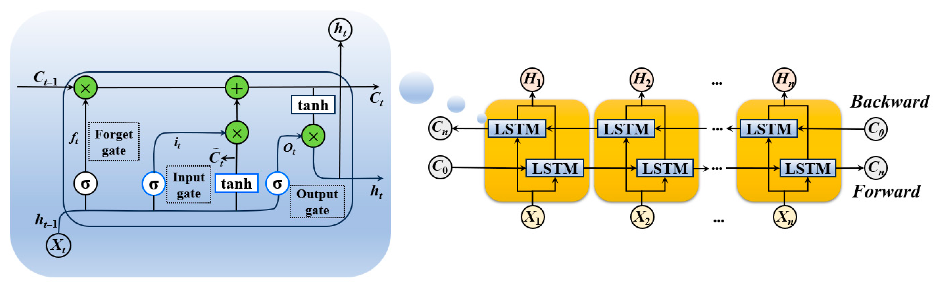
As depicted in Figure 2, the BiLSTM network features a dual-layered structure, processing sequences in both forward and reverse directions. This architectural design integrates insights from both temporal perspectives, enabling the model to capture context-sensitive representations and discern intricate temporal dependencies, particularly when the complete sequence is available during training and inference.

Within each LSTM cell, three critical gates manage information flow: the forget gate, input gate, and output gate. The forget gate determines which information from the previous cell state C_t−1 to discard, utilizing the current input x_t and previous hidden state h_t−1 with a sigmoid activation function to produce a value f_t in [0,1]. The input gate decides which new information to store in the cell state; it comprises a sigmoid function i_t to control information flow and a tanh function ${\tilde{C}}_t$ to generate candidate values. The cell state C_t is then updated by combining the forgotten old state and the new candidate information. Finally, the output gate O_t determines the cell’s final output h_t based on the current input and the updated cell state, also employing sigmoid and tanh activations. This intricate interplay of gates allows BiLSTM to robustly capture and process long-term dependencies.

CA is a mechanism designed to enhance feature representation by emphasizing informative channels and downplaying less informative ones. This technique is particularly useful in deep learning models where the sheer volume of features can obscure the most salient aspects of the data. The structure of CA is shown in Figure 3.

In the CA module, the global average pooling and global max pooling are performed on the feature map, respectively, based on the height and width, compressing the global temporal features of each channel into a 1 × 1 × C format. Then, the two compressed feature maps are input into a multi-layer perceptron (MLP) with two layers of neural networks, where the feature maps are first dimensionally reduced to 1 × 1 × C/r, and then expanded back to the original 1 × 1 × C dimension. The two feature vectors are then element-wise added, and finally, the channel attention feature weight is generated through a Sigmoid activation operation.

2.3. Bayesian Optimization

Hyperparameters are crucial to the learning process and complexity of the CNN-BiLSTM-CA model, including parameters such as the learning rate, CNN filters, and the number of BiLSTM units. Automated hyperparameter optimization not only saves time but also facilitates a fair comparison across different models [40]. BO is a robust technique for hyperparameter tuning in machine learning models. It constructs a probabilistic surrogate model of the objective function and leverages this model to guide decisions on subsequent evaluations.

In this study, Gaussian Process (GP) is adopted as the surrogate model due to its flexibility and the ability to provide uncertainty estimates. As a general paradigm for multivariate Gaussian probability distributions, the GP consists primarily of a mean function m(x) with a semi-positive definite covariance function k(x, x’), i.e.,:

$$y=gp\left(m\left(x\right),k\left(x,x^{\prime }\right)\right)$$

(4)

The general steps for prediction are depicted in Figure S1. The process commences with the initialization of the hyperparameter search space, encompassing parameters such as CNN/LSTM layer counts, unit counts in Dense/LSTM layers, learning rate, activation function, and batch size. Next, a set of initial samples is generated, from which a GP surrogate model is constructed to approximate the objective function. An acquisition function is then computed to select the next promising hyperparameter configuration, balancing exploration and exploitation. This selected configuration is evaluated against the actual objective function, and the GP surrogate model is subsequently updated with the new empirical data. This iterative cycle continues, assessing convergence criteria, until the optimal hyperparameters that maximize the objective function’s performance are output.

2.4. The CNN-BiLSTM-CA Hybrid Model

In the process of high-speed flood discharge, the vibration signals of structures exhibit not only significant temporal nonlinear characteristics but also complex spatial features in the vibration responses of various measurement points in different directions. To thoroughly analyze these characteristics, this research proposes a parallel CNN-BiLSTM-CA network model, as depicted in Figure 4. The model integrates architectures of CNN and BiLSTM with varying numbers of layers and incorporates BO for hyperparameter tuning. The CNN component leverages its robust capability for extracting nonlinear features, capturing the spatiotemporal characteristics of signals through convolutional operations, activation functions, and max pooling operations, while reducing model parameters through downsampling to prevent feature loss. On this foundation, the CNN module further integrates CA to more accurately extract key data features.

Simultaneously, the BiLSTM network is employed to synchronously capture the temporal features and long-term dependencies of structural vibration signals. The processed data is then fed into the fully connected layer of the BiLSTM, further enhancing the model’s comprehension of temporal dynamics. After these treatments, the data is flattened to fit the format required by the fully connected layer. Ultimately, the data processed by CNN and BiLSTM are concatenated in parallel as inputs to the fully connected layer, with the vertical displacement time history of the measurement points as the output, generating the corresponding temporal prediction results.

Compared with the serial CNN-BiLSTM-CA structure, the parallel CNN-BiLSTM-CA structure uses two separate branches to process the same input sequence. The CNN branch extracts local spatial correlation features, while the BiLSTM branch learns temporal dependence directly from the sequence. The two feature sets are fused only at a later stage. This helps avoid early mixing of different types of information and allows the model to preserve spatial and temporal features more effectively. As a result, the model can provide a more complete representation of the vibration response. For hydraulic structural vibration under flood discharge, where multi-point responses are coupled and change over time, this parallel design is more suitable for capturing the main characteristics of the signals.

3. Research Framework

Figure 5 shows the implementation procedure of the CNN-BiLSTM-CA model, which mainly consists of the following steps.

Step 1: Input features selection. Initial input features for predicting structural vibration were derived from three-directional displacement data collected from gantry crane beams in hydraulic engineering. Recognizing that single-sequence prediction neglects crucial spatiotemporal interactions among measurement points, thereby limiting accuracy, we considered the inherent spatiotemporal characteristics. Feature correlation was systematically assessed using both Pearson and MIC analyses, with time-lagged correction applied to enhance the robustness of these correlation results. Final input features were then meticulously selected based on their maximized Pearson and MIC coefficients.

Step 2: Data preprocessing. To generate the initial dataset for the prediction model and create the input features, the raw data undergoes preprocessing, which includes batch normalization and sliding window processing. Further details regarding these pre-processing steps are provided in Section 4.3.

Step 3: Parameter estimation. For robust neural network performance, BO is employed for hyperparameter estimation. The Root Mean Square Error (RMSE) on the test set serves as the objective function for this optimization. Based on objective function evaluations, BO constructs a probabilistic surrogate model to identify the hyperparameter combination that minimizes the RMSE, thereby yielding the optimal set.

Step 4: Optimization process explanation. PD analysis is employed to visually elucidate the BO process within selected two-dimensional hyperparameter subspaces. Concurrently, histograms illustrate the density of all sampling points across two-dimensional parameter planes, while marginal distributions depict their spread along individual dimensions. This visualization collectively facilitates the examination of hyperparameter-performance relationships, offering critical insights into the optimization landscape.

Step 5: Model prediction and performance evaluation. The CNN-BiLSTM-CA hybrid model is employed to predict the vertical displacement of the BZ51 vibration response extremum point. Model performance and generalization capabilities are validated using test set data. An ablation study assesses the model’s predictive efficacy against its constituent components (CNN, BiLSTM, and CA). Further validation involves comparative analysis with established spatiotemporal baseline models. Predictive accuracy is quantified using RMSE, Mean Absolute Error (MAE), Mean Absolute Percentage Error (MAPE), and the correlation coefficient (R), with relevant equations referenced from [37]. Superior performance is indicated by lower RMSE, MAE, and MAPE values, and a higher R value.

4. Experiment and Data

4.1. Dataset Description

The data used in this study were collected from a major hydropower project in Southwest China, which includes a concrete double-curvature arch dam, flood discharge and energy dissipation structures, and an underground water diversion and power generation system. The arch dam has a maximum height of 289 m, with a normal reservoir water level of 825 m and a crest elevation of 834 m. The power generation system features an innovative underground layout with eight 1000 MW vertical hydroelectric turbines on each bank, each with a unit diversion flow rate of 547.8 m³/s.

During flood discharge tests in October 2022, strong vibrations were observed on the upstream gate machinery platform, particularly in the simply supported beams between the spillway piers when all four deep holes were fully open. The maximum vibration acceleration reached 3 m/s². Figure S2 shows the surface discharge outlets and gantry crane beams of the project.

The analysis focuses on dam segments 16^# and 17^#, which exhibited the most intense vibrations at monitoring points BZ51 to BZ53 on the upstream gantry crane beams. These segments correspond to deep holes 2^# and 3^#, respectively. The gate machinery platform beams connect the tops of the two side piers and consist mainly of traffic beams and gantry crane beams. The critical monitoring points BZ51-BZ53, where peak vibrations were recorded, are located centrally on the top plate of the platform beams, aligned from the upstream face toward the dam body (Figure 6a shows the spillway top plate layout; Figure 6b illustrates the positions of points BZ51-BZ53). Each monitoring point records displacement in three directions. The suffix _X denotes the streamwise direction (along the river flow), _Y denotes the cross-stream direction (perpendicular to the river flow), and _Z denotes the vertical direction. For example, BZ51_Z refers to the vertical displacement at monitoring point BZ51.

4.2. Time-Lagged Correlation Study

Pearson correlation and the MIC were first used to evaluate relationships among all displacement features. Figure 7 presents the correlation heatmaps based on the original data. The Pearson coefficients for all measurement points relative to points BZ51_Z and BZ53_Z are negative, and the corresponding MIC values are relatively low, indicating weak direct correlations. These results suggest that the vibration responses may involve time lag effects that are not captured by synchronous analysis. To account for this possibility, time-lagged analysis was performed. For each candidate input feature, the lag order was searched within the range of −10 to 10 time steps. At each lag order, the shifted input sequence was aligned with the target sequence BZ51_Z, and the Pearson correlation coefficient was recalculated. The optimal lag was defined as the lag order that produced the maximum Pearson correlation coefficient with BZ51_Z. Figure 8 shows the correlation heatmap between BZ51_Z and other measurement points under different lag factors. The results indicate that displacement correlations are strongly affected by time lags. A clear periodic lag pattern is observed. The optimal lags for BZ51_X to BZ53_Y relative to BZ51_Z are {7, 4, 5, 4, 4, 6, 3, 5}, respectively. These lag values reflect the time offset at which the response at each monitoring point is most strongly correlated with the target response at BZ51_Z. Physically, the lags indicate that vibration responses at different locations do not occur at the same time. This is because flood-discharge-induced vibrations propagate along the gantry crane beam system and reach different monitoring points at different times. The transmission path, local stiffness distribution, and boundary conditions of the beam all affect how vibrations travel and develop at each point. In addition, responses in different directions (streamwise, cross-stream, and vertical) may also differ in phase due to the directional nature of the hydrodynamic loading. Therefore, the identified lag orders represent the effective time offsets caused by these combined structural and hydraulic effects, rather than simple wave travel times.

After applying the identified time lags, the Pearson and MIC coefficients were recalculated (Figure 9). The corrected Pearson coefficients increase markedly. For example, the Pearson values for BZ52_X and BZ53_Z rise to 0.50 and 0.72, respectively. In contrast, the MIC values show only slight changes. This indicates that time-lagged correction mainly improves linear correlation measures, while nonlinear correlation captured by MIC is less sensitive to temporal shifts.

Based on the corrected correlation results, the displacement of BZ51_Z was predicted using the displacement time histories of BZ52_X, BZ53_Z, and BZ53_X, which exhibited the strongest correlations. A supplementary sensitivity check indicated that small perturbations in the selected lag factors led to only limited changes in prediction performance. This suggests that the proposed model is reasonably robust to minor lag estimation errors, while the optimal lag setting still provides the best accuracy.

4.3. Data Preprocessing

In deep learning, large differences in the scale of input variables can affect model training and slow convergence. To reduce the influence of numerical scale differences and improve training stability, batch normalization is applied to the input data. This step helps standardize feature distributions and enhances computational efficiency. Meanwhile, the original vibration sequences were preserved as much as possible, so that the model could learn representative local patterns and short-term dynamic characteristics directly from the measured signals. For time-series prediction, a sliding window strategy is adopted. In this approach, several consecutive historical time steps are used as input features, and the immediately following time step is defined as the prediction target. A preliminary sensitivity analysis was conducted for different window sizes (4, 6, 8, and 10). The results showed that a window size of six achieved the best balance between prediction accuracy and model complexity, while avoiding unnecessary redundant information. Therefore, as shown in Figure S3, vibration values from the previous six time steps are used to predict the value at the next moment. This window size was determined before BO to keep the input dimensions fixed and to ensure computational efficiency during hyperparameter optimization. The window then moves forward by one time step, forming a new input sequence. This process continues until the entire dataset is processed, generating a series of overlapping sub-sequences for model training and testing.

The dataset is divided sequentially into training and testing sets using a 0.8:0.2 ratio to preserve temporal order (Figure S4). The model input consists of displacement time series from multiple monitoring points, including both X- and Z-direction responses. This multi-dimensional input structure enables the model to capture the coupled spatial characteristics of structural vibrations. The model output is the predicted Z-direction displacement at the target monitoring point (BZ51) for the next time step.

5. Prediction Results and Discussion

5.1. Parameter Estimation

Hyperparameter optimization is essential for maximizing predictive performance, particularly for deep learning models with high-dimensional search spaces. However, exhaustive approaches such as grid search are computationally expensive, and random search often yields suboptimal efficiency. BO provides a more effective alternative. By leveraging prior observations to guide the search process, BO improves sampling efficiency, especially in continuous parameter spaces and under noisy evaluations.

In this study, BO is used to optimize the key hyperparameters of the proposed neural network, including the number of CNN layers, the number and size of LSTM hidden layers, the number of Dense layer units, the learning rate, the activation function, and the batch size (Table S1). The optimization process runs for 40 iterations, and the convergence trajectory is shown in Figure S5.

Within the predefined search space (4–256), the optimal batch size is determined to be 8. Smaller batch sizes introduce greater stochasticity into gradient descent, which can help the model escape local minima, consistent with the findings of [41]. For the learning rate, the optimal value is 0.044 within the range of 0.0001–0.1. This value achieves a balance between convergence speed and training stability, and it was held constant throughout the training process. To further improve this training stability, gradient clipping was applied during optimization, complementing the inherent gating mechanism of the BiLSTM cells.

Regarding the network architecture, the optimal configuration includes three CNN layers (search range: 1–10) and ten LSTM hidden layers (search range: 1–10). ReLU is selected as the activation function due to its ability to mitigate vanishing gradient issues and facilitate stable training. In addition, 44 LSTM units (search range: 1–100) and three Dense layer units (search range: 1–80) are identified as optimal, providing sufficient model capacity while limiting the risk of overfitting. The CNN layers use a kernel size of 3 and a stride length of 1. Since the input is a multivariate time series arranged as a sliding window, the convolutional filters process the signals from all monitoring points simultaneously as parallel channels, capturing the spatial correlations and feature interactions among the different sensors.

5.2. Explainability of the BO Process

Figure 10 illustrates the BO process. The off-diagonal panels show interactions between hyperparameters, while the diagonal panels present partial dependence plots that reflect the influence of individual parameters. Dense sampling in the optimal regions (dark yellow) and sparse sampling in low-performance regions (dark blue) indicate that BO effectively uses prior evaluations to guide iterative refinement. The irregular shape of the optimal region suggests nonlinear and uneven interactions among hyperparameters in the prediction of vertical vibration at monitoring point BZ51. The figure also shows that the number of LSTM layers, LSTM units, and Dense units have relatively limited effects on prediction accuracy, whereas the number of CNN layers, learning rate, batch size, and activation function play dominant roles. Among these, the learning rate strongly affects training convergence, and the number of CNN layers has a greater influence than the depth of LSTM layers. This result highlights the importance of spatial feature extraction from multiple measurement points, especially when BZ51 is treated as an unknown target relying on spatial information from other sensors and historical records. Therefore, a multi-layer CNN structure is essential for achieving high prediction accuracy.

Figure 11 presents the distribution of all sampled points in both one-dimensional and two-dimensional projections. The diagonal panels show histograms for each parameter, while the lower triangular panels display pairwise scatter plots. Sampling order is represented by color variation, with darker purple tones indicating earlier samples and lighter yellow tones indicating later ones. The red star marks the location of the best solution found during optimization. Early samples are broadly distributed across the parameter space, whereas later samples cluster near the optimal region, demonstrating that the Bayesian optimizer progressively refines its search by building and updating a surrogate model of the parameter space.

5.3. Ablation Study

To evaluate the contribution of each module, eight model architectures are compared: BiLSTM (M1), CNN (M2), CNN-BiLSTM-Sequential (M3), CNN-BiLSTM-Parallel (M4), CA-BiLSTM-Sequential (M5), CA-BiLSTM-Parallel (M6), CNN-BiLSTM-CA-Sequential (M7), and the proposed CNN-BiLSTM-CA-Parallel (M8). All models are trained with consistent hyperparameter settings. Performance is assessed using RMSE, MAE, MAPE, and R. The results are summarized in

Table 1. Ablation experiment results.

Model	RMSE	MAE	MAPE	R
BiLSTM (M1)	10.96	7.02	0.20	97.69%
CNN (M2)	6.84	5.50	0.24	99.10%
CNN-BiLSTM-Sequential (M3)	13.68	10.94	0.52	96.40%
CNN-BiLSTM-Parallel (M4)	6.48	5.15	0.24	99.19%
CA-BiLSTM-Sequential (M5)	13.82	11.00	0.54	96.32%
CA-BiLSTM-Parallel (M6)	7.14	5.83	0.21	99.02%
CNN-BiLSTM-CA-Sequential (M7)	13.70	10.94	0.53	96.39%
CNN-BiLSTM-CA-Parallel (M8)	5.49	4.34	0.20	99.42%

and Figure S6.

The baseline CNN model (M2) already shows strong performance, achieving an R value of 99.10% with relatively low RMSE, MAE, and MAPE. Introducing a parallel CNN-BiLSTM structure (M4) slightly improves R and further reduces error metrics. When the CA module is added in the parallel architecture (M8), performance improves further, reaching the highest R value of 99.42%, with RMSE and MAE reduced from 6.48 and 5.15 to 5.49 and 4.34, respectively. In particular, the reduction in RMSE after introducing the CA module suggests that the model achieves smaller errors at locations with relatively large response amplitudes. The lower MAE also indicates a more stable overall fit. These results show that the CA module helps the model assign greater weight to informative feature channels and improves the overall fitting accuracy.

For BiLSTM-based models, adding the CA module in the parallel configuration (M6) increases R by 1.33% compared with the baseline BiLSTM model (M1) and reduces all error metrics. In general, parallel architectures (M4, M6, and M8) outperform their sequential counterparts (M3, M5, and M7), with RMSE, MAE, and MAPE reduced by nearly half. These results indicate that the parallel structure is more effective in capturing the vibration characteristics of gantry crane beams. Overall, the proposed model (M8) achieves the best performance and provides the most balanced improvement among the tested configurations.

5.4. Comparison with Baseline Models

Within the same computational environment and using identical training and testing datasets, five widely used baseline models, including XGBoost, SVM, Kernel Ridge (KR), Random Forest (RF), and Bidirectional Temporal Convolutional Network (BiTCN), are selected for comparison. Their main hyperparameters are listed in

Table 2. Parameter settings of the baseline models.

Model	Parameter Settings
XGBoost	nestimators = 500, lr = 0.08, max_depth = 7
SVM	C = 1.0, γ = 0.5
Kernel Ridge	Kernel = RBF, γ = 0.1
Random Forest	nestimators = 60
BiTCN	nfilters = 64, Kernel_size = 2
Proposed	CNN (3 layers), BiLSTM (10 layers, 44 neurons)

. XGBoost is configured with 500 estimators, a learning rate of 0.08, and a maximum depth of 7. SVM uses C = 1.0 and γ = 0.5. KR adopts a radial basis function kernel with γ = 0.1. RF contains 60 estimators to improve model generalization. BiTCN employs 64 filters with a kernel size of 2 to capture local temporal features. The proposed model uses the optimized configuration identified earlier, including three CNN layers and ten BiLSTM layers with 44 units each. All models are applied to predict the Z-direction vibration sequence at monitoring point BZ51, and the predicted results are compared with measured values (Figure 12).

All models capture the general trend of the vibration response, but SVM, KR, and RF show clear phase lag near sharp peaks, as highlighted in the enlarged views in Figure 12. XGBoost provides better phase alignment but lower overall accuracy. BiTCN and the proposed CNN-BiLSTM-CA model achieve closer agreement with measured data, with the proposed model showing the best overall fit and the highest prediction accuracy. These results indicate that the hybrid framework more effectively learns complex temporal and spatial patterns in the vibration signals.

Prediction performance is further evaluated using absolute error, RMSE, MAE, MAPE, and R, as shown in Figure 13. SVM has the widest error distribution and the highest median absolute error, followed by KR, RF, and XGBoost. By contrast, BiTCN and the proposed model show much lower median errors and more concentrated distributions, indicating better prediction stability. Among them, the proposed model still performs better, especially in some regions with relatively large response changes, as also reflected in Figure 12. This difference may be attributed to the feature learning strategy. BiTCN mainly uses convolution-based operations for sequence modeling, while the proposed CNN-BiLSTM-CA model further combines local feature extraction, temporal dependence learning, and adaptive channel weighting. This helps the model better capture the coupled spatial-temporal characteristics of structural vibration signals. Figure 13b further compares the overall performance metrics, showing that SVM produces error values more than twice those of the proposed model. In terms of computational cost, all models can complete training within about 2–3 s under the present data scale, and the time differences among models are small. Although the proposed M8 model requires slightly more training time, this increase is very limited, while the improvement in prediction accuracy is more evident. Overall, the proposed model demonstrates the most accurate and stable prediction performance among all baseline models, with a performance improvement of up to 50% over baseline models.

6. Conclusions

This study proposes a CNN-BiLSTM-CA parallel network to predict gantry crane beam displacements during high-speed flood discharge. The framework integrates time-lagged Pearson correlation and MIC for feature selection, CNN for spatial feature extraction, BiLSTM for bidirectional temporal modeling, and a CA mechanism to enhance nonlinear feature representation. BO is applied to tune hyperparameters, and PD analysis is used to interpret parameter effects. The model is validated using experimental data from an arch dam in Southwest China, and performance is evaluated using RMSE, MAE, MAPE, and R. The main findings are as follows:

(1)

Time-lagged correction significantly improved Pearson correlation values, indicating stronger linear relationships, while MIC values showed smaller changes. This suggests that time lag is more critical for linear dependencies, whereas nonlinear relationships remain relatively stable.

(2)

BO efficiently optimized key hyperparameters. CNN depth, learning rate, batch size, and activation function had the greatest influence on performance. CNN parameters affected prediction accuracy more than LSTM parameters, highlighting the importance of spatial feature extraction. Optimal performance was achieved with three CNN layers, a learning rate of 0.044, a batch size of 8, and ReLU activation.

(3)

Ablation study demonstrated that the integrated CNN-BiLSTM-CA model outperformed individual CNN, BiLSTM, and sequential baseline models. The parallel structure prevented information from mixing too early and improved prediction accuracy.

(4)

Compared with baseline methods, the proposed model reduced RMSE, MAE, and MAPE by up to 50% and closely matched measured vibration responses, demonstrating strong capability in capturing complex structural dynamics during flood discharge.

Future work can be carried out in the following aspects. First, the proposed model should be further validated using vibration data from more hydropower projects and a wider range of discharge conditions, so that its generalization ability can be examined more fully. Second, additional influencing factors, such as discharge flow, gate opening, and other hydraulic variables, may be introduced to better describe the coupling between structural vibration and hydraulic loading. Third, future studies can further improve the model in terms of interpretability and engineering applicability, so that the prediction results can provide more direct support for vibration monitoring and safety assessment.