FEA-Based Vibration Modal Analysis and CFD Assessment of Flow Patterns in a Concentric Double-Flange Butterfly Valve Across Multiple Opening Angles

Abstract

A concentric double-flange butterfly valve (DN-500, PN-10) was analyzed to examine its dynamic behavior and internal fluid flow across multiple opening angles. Finite Element Analysis (FEA) was employed to determine natural frequencies, mode shapes, and effective mass participation factors (EMPFs) for valve positions at 30°, 60°, and 90°. The valve geometry was discretized using a curvature-based mesh with linear elastic isotropic properties for 1023 carbon steel. Lower-order vibration modes produced global deformations primarily along the valve disk, while higher-order modes showed localized displacement near the shaft–bearing interface, indicating coupled torsional and translational dynamics. The highest EMPF in the X-direction occurred at 1153.1 Hz with 0.2631 kg, while the Y-direction showed moderate contributions peaking at 0.1239 kg at 392.06 Hz. The Z-direction demonstrated lower influence, with a maximum EMPF of 0.1218 kg. Modes 3 and 4 were critical for potential resonance zones due to significant mass contributions and directional sensitivity. Computational Fluid Dynamics (CFD) simulation analyzed flow behavior, pressure drops, and turbulence under varying valve openings. At a lower opening angle, significant flow separation, recirculation zones, and high turbulence were observed. At 90°, the flow became more streamlined, resulting in a reduction in pressure losses and stabilizing velocity profiles.

1. Introduction

Butterfly valves are widely used in industrial flow control systems due to their compact structure, low cost, and operational efficiency. These valves are particularly favored in applications involving large diameters and moderate pressure ratings, such as water distribution, chemical processing, and power generation. Despite their structural simplicity, butterfly valves are subject to complex dynamic phenomena arising from Fluid–Structure Interactions, mechanical excitation, and operational variations, which can compromise their functional performance and structural integrity over time. The dynamic behavior of butterfly valves is critical, especially under cyclic loading or fluctuating flow conditions, where resonant vibrations may lead to fatigue, deformation, or failure. Modal analysis provides a systematic approach for characterizing the inherent vibrational properties of such components, enabling the identification of natural frequencies, deformation patterns (mode shapes), and their sensitivity to structural and operational parameters. These modal characteristics are essential for predicting the valve’s response to dynamic loads and for designing mitigation strategies against resonance-induced failure. The identification of vibration modes and effective mass participation in a concentric double-flange butterfly valve at various opening angles can be effectively analyzed using Finite Element Analysis (FEA) and Fluid–Structure Interaction (FSI) methodologies. FEA is a powerful tool for assessing the structural stability and dynamic behavior of butterfly valves, as demonstrated in studies that focus on shape optimization and material analysis to enhance valve performance [1,2,3]. The nonlinear dynamic behavior of flange-bolted joints, as discussed by Shi and Zhang, highlights the importance of considering contact nonlinearity and preload performances in the vibration analysis of such systems [4]. The comparative study by Wu et al. on butterfly valves emphasizes the significance of valve opening angles on flow characteristics, which directly influence the vibration modes due to changes in flow-induced forces [5]. Vibration analysis, as reviewed by Chu et al., is crucial for predictive maintenance and fault diagnosis, suggesting its applicability in monitoring the health of butterfly valves in fluid systems [6]. Tripathi et al. demonstrate the utility of FEA-based vibration analysis in shipboard piping systems, which can be adapted to analyze the dynamic response of butterfly valves under varying operational conditions [7]. Morales et al. provide insights into FSI analysis, which is essential for understanding the interaction between fluid flow and valve structure, particularly at different opening angles, affecting the valve’s vibration characteristics [8]. The study by Huang et al. on dominant vibration modes in machine tools can be extrapolated to identify dominant modes in butterfly valves, where certain modes may dominate depending on the valve’s opening angle and flow conditions [9]. Attia et al. discuss the significance of complex mode shapes in pipes conveying fluids, which can be applied to understand the vibration modes of butterfly valves, especially under compressible flow conditions [10]. The integration of CFD and FEA, as explored by Abuhatira et al., provides a robust framework for predicting structural responses and identifying potential leak points, which is relevant for assessing the integrity and performance of butterfly valves under dynamic conditions [11]. Finally, the efficient space–time FEA strategy by Dyniewicz et al. offers a computationally efficient approach to solving large-scale vibration problems, which can be beneficial for analyzing the complex dynamics of butterfly valves in industrial applications [12]. Valves in pipeline systems exposed to external excitations with frequencies coinciding with the system’s natural modes can significantly accelerate wear and contribute to structural failure [13,14,15]. Furthermore, the effective mass factor, quantified for each vibrational mode, serves as a critical indicator of how the system mass is distributed across the modal responses [16].

In light of structural complexities and fluid-induced forces inherent in the operation of butterfly valves, the present study aims to investigate the modal behavior of a concentric double-flange butterfly valve using Finite Element Analysis and Computational Fluid Dynamics. The primary focus is on quantifying natural frequencies, identifying mode shapes, evaluating effective mass participation, and analyzing flow characteristics, pressure distributions, and turbulence patterns across three valve opening angles. By examining the directional influence of vibrational modes and their potential to induce resonance, this study provides critical understanding for improving valve design, ensuring mechanical integrity, and enhancing dynamic performance in fluid control systems. The outcomes of this study may serve as a foundation for developing mitigation strategies against dynamic instabilities and guiding future optimization of industrial valve structures under dynamic flow conditions.

2. Modal and Effective Mass Participation Analysis of a Butterfly Valve

Modal analysis of a butterfly valve (DN-500 PN-10 concentric double-flange butterfly valve) using Finite Element Analysis (FEA) involves analyzing the entire geometry of the valve for dynamic behavior, and the entire structure is subdivided into small elements. FEA is a numerical way of solving complex structural problems, especially in the area of modal analysis. In the case of a butterfly valve shown in Figure 1, this analysis assists in determining the resonance vibrations all along the system to enable the design to do away with such concerns. The examination encompasses computations pertaining to the inherent frequencies and mode shapes of the valve structure, which serve as instrumental resources for forecasting the response of the system to diverse loading conditions.

By omitting the effect of damping and external excitation, the general linear equation governing the motion of the butterfly valve system can be written as follows:

$$\left[M_{ij}\right]\left\{{\ddot{u}}_j\right\}+\left[K_{ij}\right]\left\{u_j\right\}=\left\{0\right\}\hspace{0.17em}\hspace{0.17em}\hspace{0.17em}\hspace{0.17em}\hspace{0.17em}\hspace{0.17em}\hspace{0.17em}\hspace{0.17em}\hspace{0.17em}\hspace{0.17em}\hspace{0.17em}\hspace{0.17em}\hspace{0.17em}\hspace{0.17em}\hspace{0.17em}\hspace{0.17em}\hspace{0.17em}\hspace{0.17em}i,j=1,2,\dots ,n$$

(1)

where M_ij represents the mass and K_ij represents stiffness. Assuming the displacement varies harmoniously with respect to time, the displacement $u_i$ and acceleration ${\ddot{u}}_i$ factors can be expressed as follows:

$$u_i(x,t)={\varphi }_i(x)\sin \left({\omega }_{i}t+{\theta }_i\right)$$

(2)

$${\ddot{u}}_i(x,t)=-{\omega }_i^2{\varphi }_i(x)\sin \left({\omega }_{i}t+{\theta }_i\right)$$

(3)

where ${\varphi }_i(x)$ is the modal displacement vector; substituting (2) and (3) into (1) yields the following:

$$\left(\left[K\right]-{\omega }_i^2\left[M\right]\right)\left\{{\varphi }_i(x)\right\}=\left\{0\right\}$$

(4)

The EMPF measures the proportion of the total mass of the system that contributes to the dynamic response in a given direction for that mode. It indicates how much mass of the system participates in the vibration for a particular mode and can mathematically be represented as follows:

$$EMPF={{\displaystyle \frac{\left({\displaystyle {\sum }_j{m}_j{\varphi }_{i,i}}\right)}{{\displaystyle {\sum }_j{m}_j{\varphi }_{j,i}^2}}}}^2$$

(5)

where m_j is the mass of the j-th degree of freedom and ϕ_j,i is the mode shape value for the j-th degree of freedom in mode i.

Table 1. Material properties of the FEA model.

Material	1023 Carbon Steel
Model type	Linear Elastic Isotropic
Failure criterion	Max von Mises Stress
Yield strength	283 MPa
Tensile strength	425 MPa
Mass density	7858 kg/m3
Young’s modulus	205 GPa
Poisson’s ratio	0.29

presents an extensive compilation of the pertinent parameters that characterize the material properties employed within the context of the Finite Element Analysis.

In this analysis, the renowned software Solidworks version 2023 was meticulously utilized as the Finite Element Analysis tool, which facilitated the intricate process of discretizing the model into a multitude of small, manageable elements, thereby enabling a highly accurate and detailed simulation of the complex geometry associated with the butterfly valve.

Table 2. Meshing information of FEA.

Mesh Type	Solid Mesh
Mesh type	Blended curvature-based mesh
High-quality mesh based on Jacobian points	16 points
Maximum element size	18.2467 mm
Minimum element size	0.912334 mm
Maximum aspect ratio	1.8454 × 105
% of elements with aspect ratio < 3	93
% of elements with aspect ratio > 10	0.758
Quality of mesh	High

presents the full specifications of the different meshing types applied in the Finite Element Analysis of the valve configuration. A refined discretization strategy employing a small minimum element size was adopted to enhance the geometric fidelity of the valve domain, allowing an accurate representation of local features and fine structural details.

Linear tetrahedral elements were assessed using Jacobian points, which served as reference landmarks for evaluating the mesh quality throughout the structure. The mesh generation process incorporated a curved-type meshing technique, selected specifically to account for the valve’s complex curvature and to ensure the formation of smoothly contoured elements.

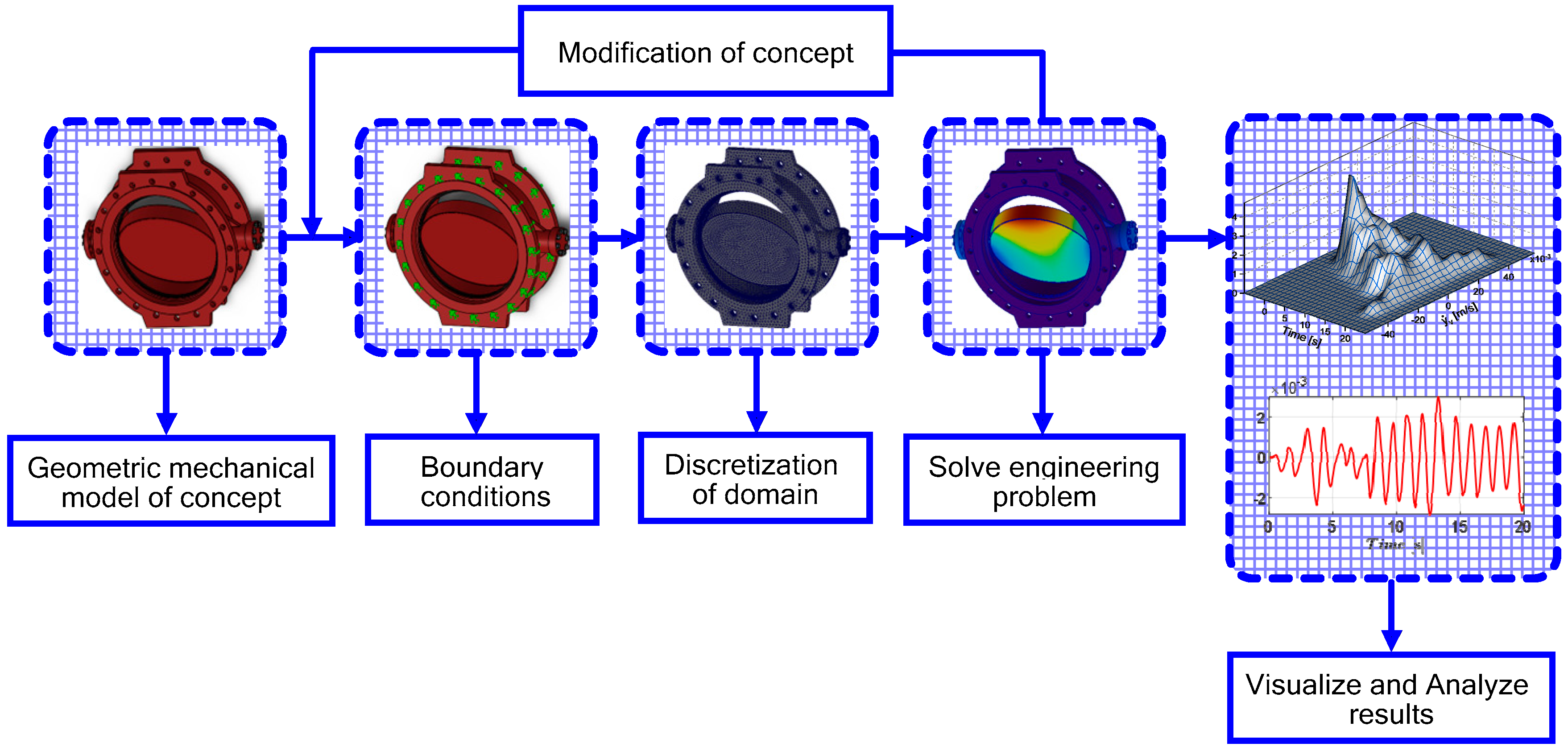
Figure 2 illustrates the flowchart delineating the sequential steps involved in the modal Finite Element Analysis process pertaining to the butterfly valve system. The execution of Finite Element Analysis encompasses three distinct phases of activity: (1) preprocessing, (2) processing, and (3) postprocessing.

Preprocessing involves the geometric mechanical model of the butterfly valve concept, such as nodal coordinates, element connectivity, boundary conditions where the flanges are constrained to move, and material properties assigned to the model. An adaptive mesh was generated in the discretization of a domain to produce nodal coordinate data and optimal node numbering, as well as element connectivity data. Jacobian points served as reference landmarks to assess the quality of each mesh constructed with linear tetrahedral elements. In the processing stage, the finite element program processed the input data and solved an eigenproblem by incremental techniques. The resulting color gradient illustrates the spatial variation in the deformation field, enabling visualization of local deformation intensities across the domain. In the postprocessing, visualization and results were presented by producing displays of the deformed configuration and vibration mode shapes of the system.

3. Computational Fluid Dynamics of a Butterfly Valve System

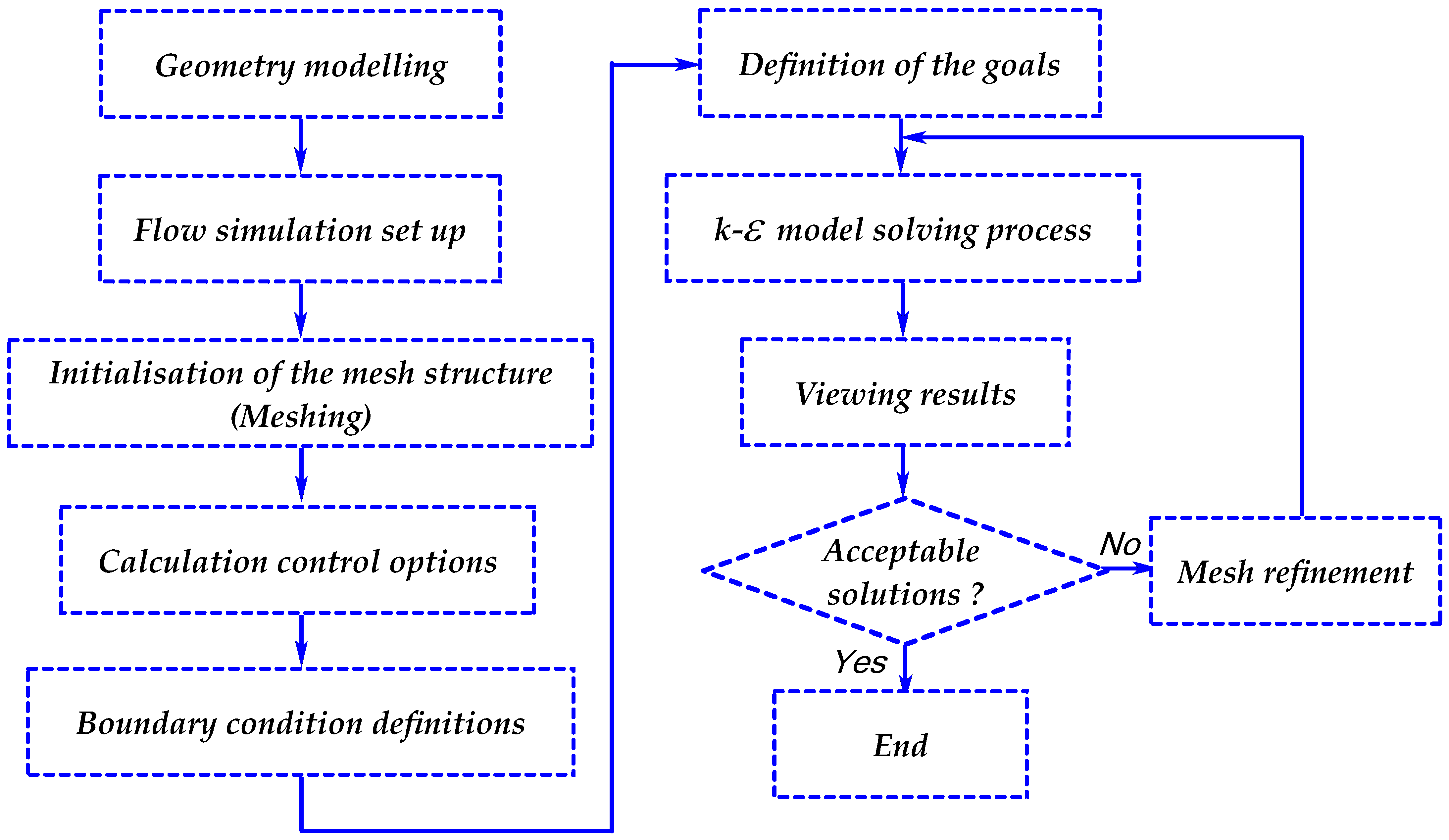
Computational Fluid Dynamics (CFD) provides a numerical framework to analyze the behavior of fluid flow through a butterfly valve system, capturing detailed patterns of velocity, pressure, and turbulence that develop across different valve opening angles. A butterfly valve introduces significant flow disturbances due to the presence of the rotating disk, which modifies the internal geometry and generates complex flow separation zones, recirculation regions, and variations in pressure distribution. The Iterative Time Advancement Solution Method presented in the flowchart in Figure 3 is a numerical approach employed as a fundamental technique in CFD simulation. This method is particularly associated with segregated solvers, which are a class of algorithms that iteratively solve equations for different physical quantities in a segregated or decoupled manner.

In fluid dynamics, the extensive form of conservation of momentum can be expressed through the Navier–Stokes equations. These equations are derived from the principle of momentum conservation and incorporate the effects of pressure gradients, fluid inertia, and Reynolds stress terms.

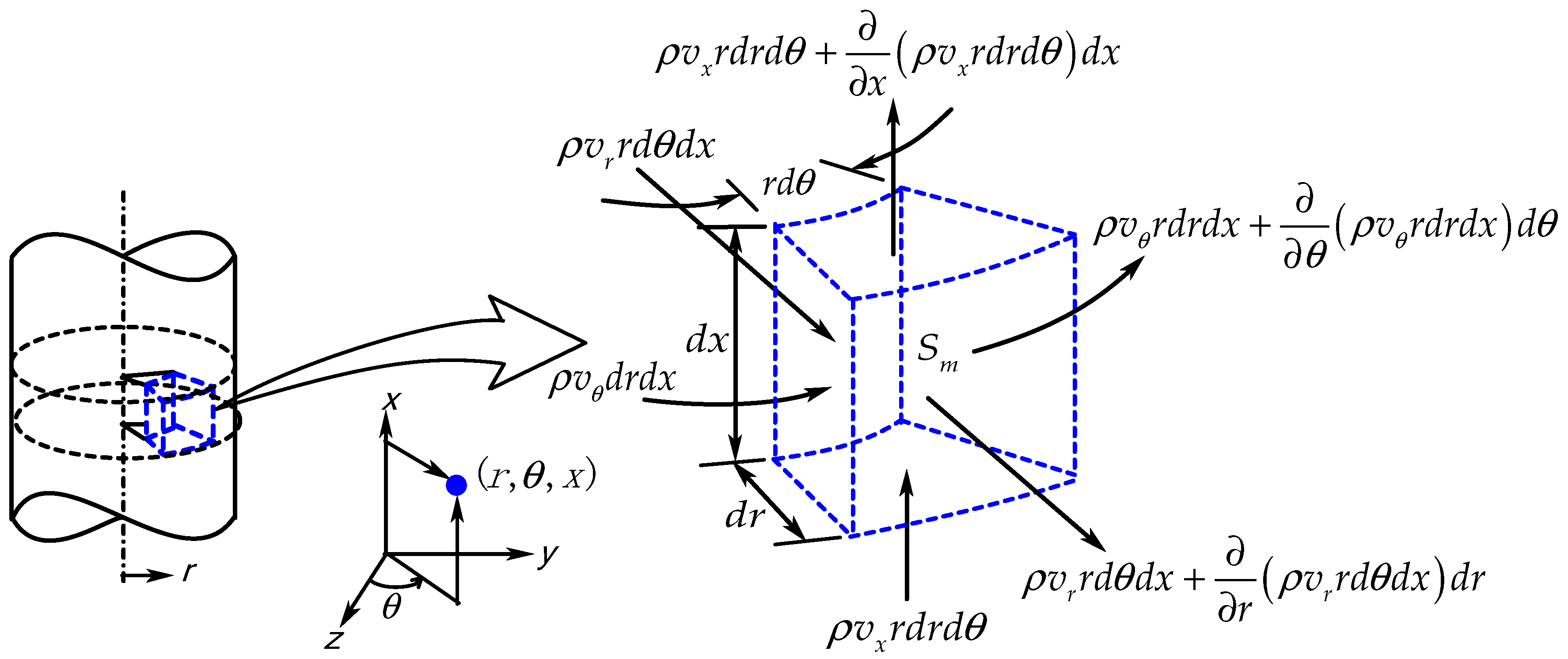
To ensure the balance of mass within a fluid system of a cylindrical control volume of three-dimensional flow shown in Figure 4, the fundamental principle of continuity is applied. The cylindrical finite volume illustrates the spatial extent of the three-dimensional flow. The blue dashed lines indicate the boundaries of the control volume, and the arrows represent mass flux terms in the cylindrical coordinate system r, θ and x.

When examining two-dimensional axisymmetric flows, the subsequent representation of the continuity equation can be employed.

$${\displaystyle \frac{\partial v_r}{\partial t}}+v_r{\displaystyle \frac{\partial v_r}{\partial r}}+{\displaystyle \frac{v_{\theta }}{r}}{\displaystyle \frac{\partial v_r}{\partial \theta }}-{\displaystyle \frac{v_{\theta }^2}{r}}+v_x{\displaystyle \frac{\partial v_r}{\partial x}}=-{\displaystyle \frac{\partial p}{\partial r}}+F_r$$

(6)

$$F_r={\displaystyle \frac{\partial {\overline{{v^{\prime }}_r{v}^{\prime }}}_r}{\partial r}}+{\displaystyle \frac{1}{r}}{\displaystyle \frac{\partial {\overline{{v^{\prime }}_r{v}^{\prime }}}_{\theta }}{\partial r}}+{\displaystyle \frac{\partial {\overline{{v^{\prime }}_r{v}^{\prime }}}_r}{\partial x}}+{\displaystyle \frac{{\overline{{v^{\prime }}_{\theta }{v}^{\prime }}}_{\theta }}{r}}$$

(7)

$${\displaystyle \frac{\partial v_{\theta }}{\partial t}}+v_r{\displaystyle \frac{\partial v_{\theta }}{\partial r}}+{\displaystyle \frac{v_{\theta }}{r}}{\displaystyle \frac{\partial v_{\theta }}{\partial \theta }}+{\displaystyle \frac{v_r{v}_{\theta }}{r}}+v_x{\displaystyle \frac{\partial v_{\theta }}{\partial x}}=-{\displaystyle \frac{1}{r}}{\displaystyle \frac{\partial p}{\partial \theta }}+F_{\theta }$$

(8)

$$F_{\theta }={\displaystyle \frac{\partial {\overline{{v^{\prime }}_{\theta }{v}^{\prime }}}_r}{\partial r}}+{\displaystyle \frac{1}{r}}{\displaystyle \frac{\partial {\overline{{v^{\prime }}_{\theta }{v}^{\prime }}}_{\theta }}{\partial \theta }}+{\displaystyle \frac{\partial {\overline{{v^{\prime }}_{\theta }{v}^{\prime }}}_x}{\partial x}}-{\displaystyle \frac{{\overline{{v^{\prime }}_r{v}^{\prime }}}_{\theta }}{r}}$$

(9)

$${\displaystyle \frac{\partial v_x}{\partial t}}+v_r{\displaystyle \frac{\partial v_x}{\partial r}}+{\displaystyle \frac{v_{\theta }}{r}}{\displaystyle \frac{\partial v_x}{\partial \theta }}+v_x{\displaystyle \frac{\partial v_x}{\partial x}}=-{\displaystyle \frac{\partial p}{\partial x}}+F_x$$

(10)

$$F_x={\displaystyle \frac{\partial {\overline{{v^{\prime }}_x{v}^{\prime }}}_r}{\partial r}}+{\displaystyle \frac{1}{r}}{\displaystyle \frac{\partial {\overline{{v^{\prime }}_x{v}^{\prime }}}_{\theta }}{\partial \theta }}+{\displaystyle \frac{\partial {\overline{{v^{\prime }}_x{v}^{\prime }}}_x}{\partial x}}$$

(11)

In the radial direction, the Equations of momentum, (6) and (7), govern the motion inside or outside of the perpendicular fluid to the axis of the valve. It is responsible for the form as the speed radial seedling along the time and of the space due to the inertia, pressure gradients, and interactions with rotational or axial directions. A centrifugal force, resulting from the curvature of the cylindrical system, balances the effects of the rotation of the fluid, while the turbulence through the Reynolds stresses redistributes the momentum in the radial plane. Equations (8) and (9) accompany the alterations in the azimuthal velocity due to the pressure gradients, the entrances, and the coupling between rotational and radial flow. The turbulence contributes to the transfer of the angular momentum through the shear stresses, influencing the whirl behavior and the stability of the fluid. Equations (10) and (11) reflect the form as the axial speed responds to the pressure gradients that drive the flow and the interaction between radial and azimuthal velocities. The Reynolds stresses induced by the turbulence redistribute the axial momentum, affecting the velocity profile and the resistance to flow. The butterfly valve introduces a localized pressure drop and modifies the axial flow by altering the flow area, increasing the complexity of the system.

The Reynolds stress tensor $-\overline{{v^{\prime }}_i{v^{\prime }}_j}$ models the turbulence. Using the Boussinesq approximation, it is expressed as follows:

$$-\overline{{v^{\prime }}_i{v^{\prime }}_j}={\nu }_t\left({\displaystyle \frac{\partial {\overline{v}}_i}{\partial x_j}}+{\displaystyle \frac{\partial {\overline{v}}_j}{\partial x_i}}\right)-{\displaystyle \frac{2}{3}}k{\delta }_{ij}$$

(12)

$${\nu }_t=C_{\mu }{\displaystyle \frac{k^2}{\epsilon }}, k={\displaystyle \frac{1}{2}}\overline{{v^{\prime }}_i{v^{\prime }}_i} \mathrm{and} {\delta }_{ij}=\left\{\begin{array}{c}1\hspace{0.17em}\hspace{0.17em}if\hspace{0.17em}\hspace{0.17em}i=j\hspace{0.17em}\hspace{0.17em}\hspace{0.17em}\hspace{0.17em}\hspace{0.17em}\\ 0\hspace{0.17em}\hspace{0.17em}otherwise\end{array}\right.$$

The k-ε turbulence model is represented by an equation that offers a method of solving the turbulent kinetic energy (k) and the rate of dissipation of turbulent kinetic energy (ε). The two quantities are essential for the characterization of turbulent flow and can be used to give a fairly good estimation of the effects of turbulence.

$${\displaystyle \frac{\partial k}{\partial t}}+v_j{\displaystyle \frac{\partial k}{\partial x_j}}={\nu }_t\left({\displaystyle \frac{\partial v_i}{\partial x_j}}+{\displaystyle \frac{\partial u_j}{\partial x_j}}\right){\displaystyle \frac{\partial v_i}{\partial x_j}}-\epsilon +{\displaystyle \frac{\partial }{\partial x_j}}\left[\left(\nu +{\displaystyle \frac{v_t}{{\sigma }_k}}\right){\displaystyle \frac{\partial k}{\partial x_j}}\right]$$

(13)

$${\displaystyle \frac{\partial ϵ}{\partial t}}+v_j{\displaystyle \frac{\partial ϵ}{\partial x_j}}=C_{1\epsilon }{\displaystyle \frac{\epsilon }{k}}{\nu }_t\left({\displaystyle \frac{\partial v_i}{\partial x_j}}+{\displaystyle \frac{\partial u_j}{\partial x_j}}\right){\displaystyle \frac{\partial v_i}{\partial x_j}}-C_{2\epsilon }{\displaystyle \frac{{\epsilon }^2}{k}}+{\displaystyle \frac{\partial }{\partial x_j}}\left[\left(\nu +{\displaystyle \frac{{\nu }_t}{{\sigma }_{\epsilon }}}\right){\displaystyle \frac{\partial ϵ}{\partial x_j}}\right]$$

(14)

4. Results and Discussion

In this section, the numerical results obtained from FEA conducted on the concentric double-flange butterfly valve system under three configurations of opening valve position angles (30°, 60°, and 90°) are presented. Emphasis is placed on the dynamic response characteristics, including natural frequencies, deformation mode shapes, and EMPFs for evaluating potential resonance phenomena associated with structural vulnerabilities and their directional dependence.

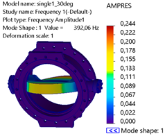
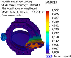
Table 3. The first six natural frequency mode shape deformations at a 30° valve opening.

illustrates the deformation patterns and amplitude resultant (AMPRES) across all directions (X, Y, and Z) of the first six natural frequency mode shapes at a 30° valve opening. Mode 1 with 392.06 Hz exhibits the highest AMPRES at the central disk region, indicating a dominant response in the translational direction. This mode likely corresponds to the primary bending behavior of the valve. Mode 3 with 912.21 Hz shows significant deformation at the periphery of the disk, indicating a localized response to higher vibrational frequencies. Mode 6 with 1153.1 Hz exhibits high AMPRES along the shaft–bearing interface of the valve, indicating torsional and coupled behaviors.

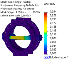
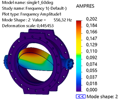
Table 4. The first six natural frequency mode shape deformations at a 60° valve opening.

displays the first six natural frequency mode shape deformations at a 60° valve opening. The deformation patterns and AMPRES are analyzed across the X, Y, and Z directions. The natural frequencies range from 382 Hz at mode 1 to 1125 Hz at mode 6. The frequency increases with higher mode shapes, reflecting more localized and higher-order deformation patterns. Lower modes (modes 1 and 2) exhibit dominant global deformation, while higher modes (modes 5 and 6) show localized effects and coupled dynamics. In

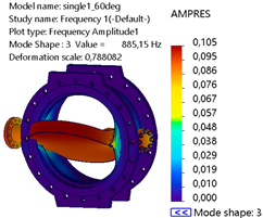
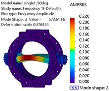
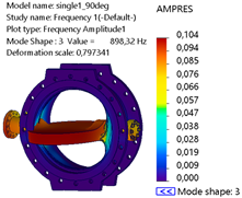
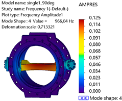
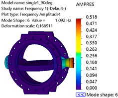
Table 5. The first six natural frequency mode shape deformations at a 90° valve opening.

, mode 1 at 394.89 Hz exhibits significant global bending, with a noticeable deformation at the lower and upper edges of the disk region. AMPRES is relatively high, indicating a dominant response in the X-direction. Mode 2 at 572.51 Hz displays asymmetrical deformation, with a combination of bending and torsional effects. AMPRES emphasizes the onset of coupled behavior in this mode. Mode 3 at 803.82 Hz predominantly shows localized deformation at the valve disk and shaft–bearing interface, with a decrease in AMPRES compared to lower modes, but localized stress regions are critical for fatigue analysis. Mode 4 at 966.04 Hz shows more complex patterns of deformation, with contributions from both translational and torsional motions.

The AMPRES is lower compared to mode 1 but reflects critical regions of stress accumulation. Mode 5 at 1072.7 Hz shows high-frequency localized deformation concentrated specifically at the shaft–bearing interface. Mode 6 at 1092 Hz exhibits the highest torsional deformation, with a sharp increase to the largest AMPRES observed among all modes, indicating critical susceptibility to high-frequency excitations at the shaft–bearing interface of the valve. 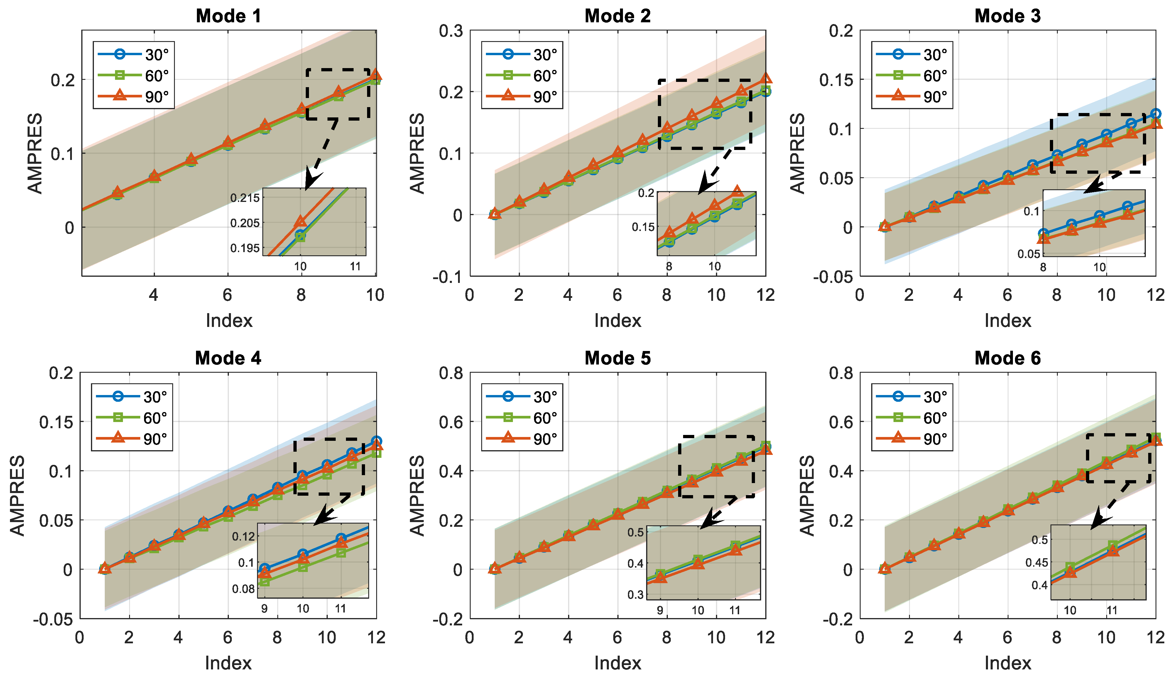Figure 5 presents the mean AMPRES responses and associated standard deviation envelopes for valve opening angles of 30°, 60°, and 90° across six vibration modes. The results indicate a clear trend of increasing AMPRES with both mode number and valve opening angle.

The 90° configuration exhibits high deformation amplitudes in modes 1 and 2, indicating increased susceptibility to resonance and dynamic amplification. The 30° opening consistently shows dominance at modes 3 and 4, indicating greater vibrational sensitivity. The 60° configuration lies between the two extremes but demonstrates lower dominance across the modes, with more evidence in modes 5 and 6. The widening of standard deviation bands in higher modes reflects greater variability and structural complexity, likely due to the localized and coupled nature of higher-order mode shapes.

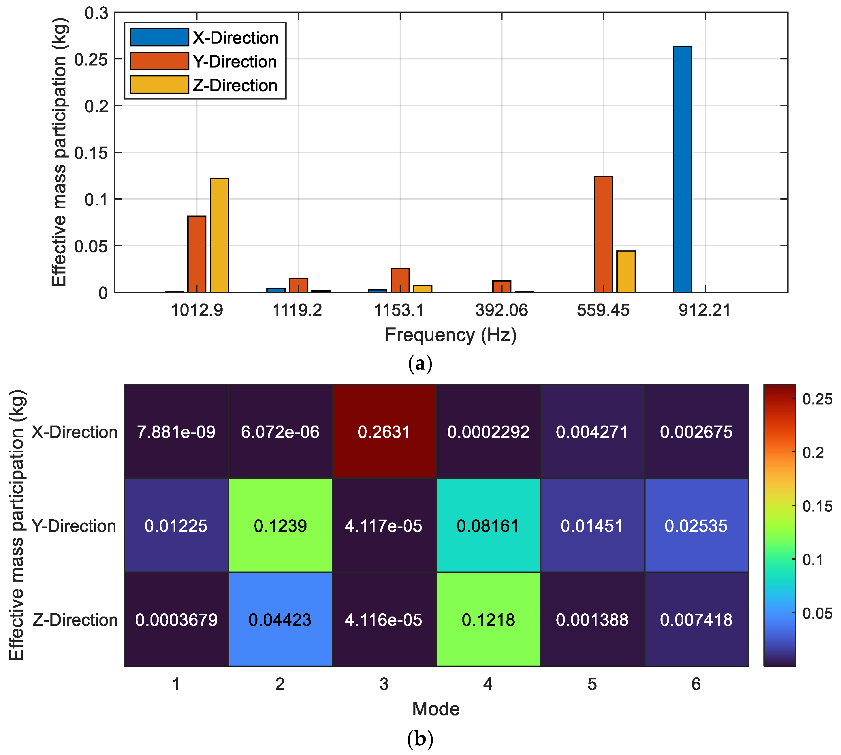
The EMPF of a 30° valve opening was analyzed as a function of the resonance frequencies, as shown in Figure 6a, and consequently presented as a heatmap for different oscillating modes across the X, Y, and Z directions in Figure 6b. The X-direction exhibits the highest EMPF at specific resonance frequencies, particularly at frequencies of 1153 Hz and 912 Hz, indicating oscillatory motion along the X-direction for high structural sensitivity. The Y-direction shows moderate participation, particularly at 392 Hz and 559, implying that these frequencies are primarily affected by motions along the Y-axis. The Z-direction has relatively low participation across the analyzed frequencies, indicating limited impact in this direction. The system might require damping mechanisms in directions and frequencies with high EMPF values to mitigate resonance effects. The heatmap highlights significant EMPF values for the X-direction in mode 3, with a peak value of 0.2631 kg, and in mode 4, with a value of 0.08161 kg. The Y-direction shows its highest EMPF in mode 2 with 0.1239 kg and mode 4 with 0.08161 kg. The Z-direction shows relatively lower values across all modes, with the highest EMPF of 0.1218 kg in mode 4. However, these contributions remain less significant compared to the X and Y directions. The heatmap reveals clear distinctions in mode participation, with mode 3 and mode 4 showing higher contributions in all three directions compared to other modes.

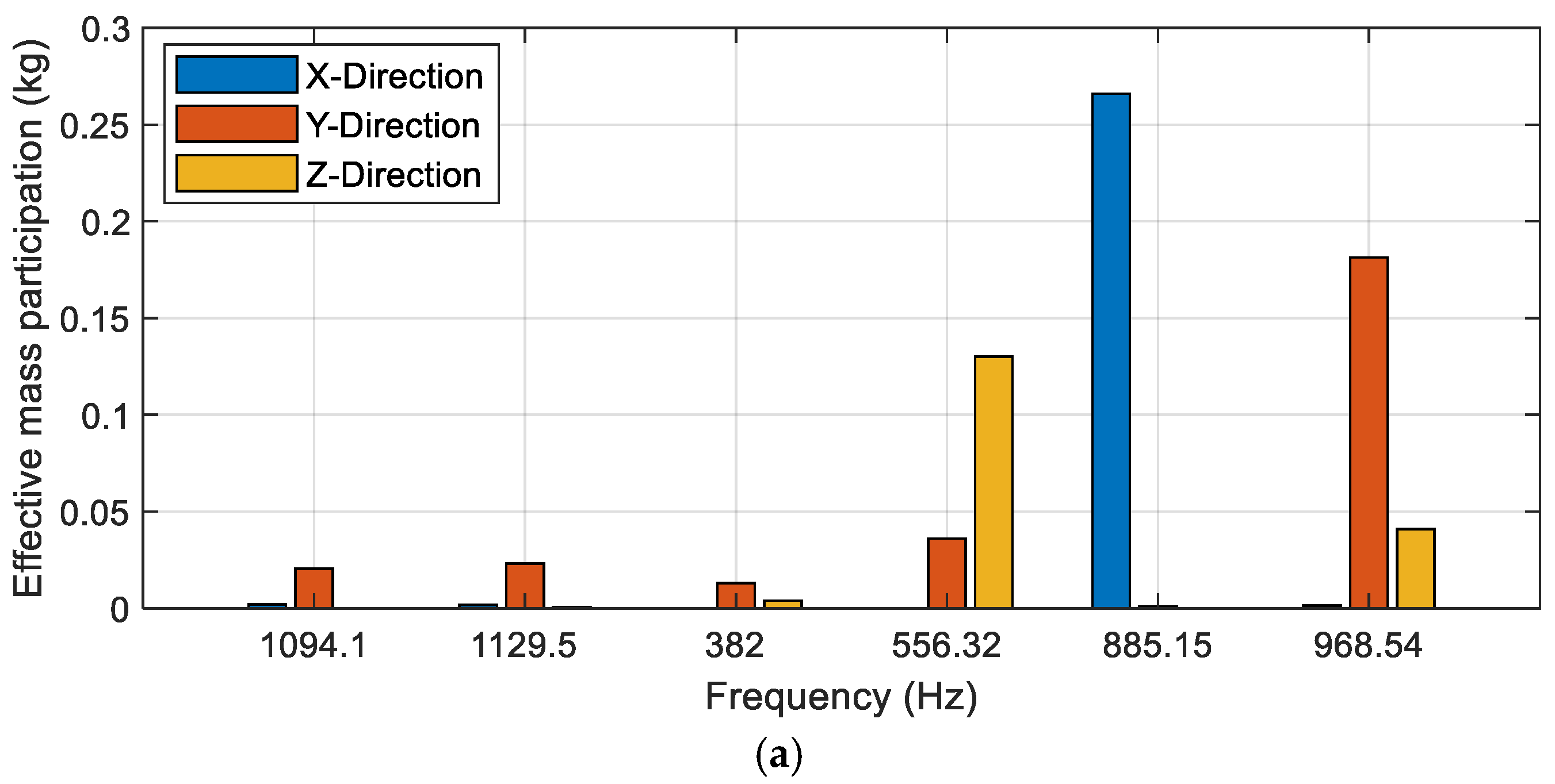
In Figure 7a, similar to the 30° opening, the X-direction exhibits the highest EMPF at certain frequencies, particularly at 1094 Hz and 885 Hz, highlighting that the system is highly sensitive to oscillatory motion along the X-axis for these resonance frequencies. The peak value in the X-direction at 1094 Hz with 0.266 kg indicates that this frequency is critical and may require mitigation strategies to avoid excessive vibrations. At 556 Hz, the Y-direction shows significant participation; the motion along the Y-axis is predominant, indicating a directional shift in dynamic behavior, where Y-axis vibrations are more pronounced than in other directions for this specific frequency. The Z-direction shows noticeable EMPF at 969 Hz. Although its contribution is less significant compared to the X and Y directions, it becomes prominent at specific frequencies, indicating a non-negligible effect. In Figure 7b, mode 2 in the X-direction shows the highest EMPF of 0.266 kg, indicating that this mode dominates the dynamic response in this direction, aligning with the observations in the frequency analysis. The Y-direction at mode 4 exhibits the highest EMPF of 0.1812 kg, making this mode significant for motion along the Y-axis. At mode 3, the Z-direction shows the highest EMPF of 0.1301 kg, demonstrating that this mode predominantly affects Z-axis dynamics.

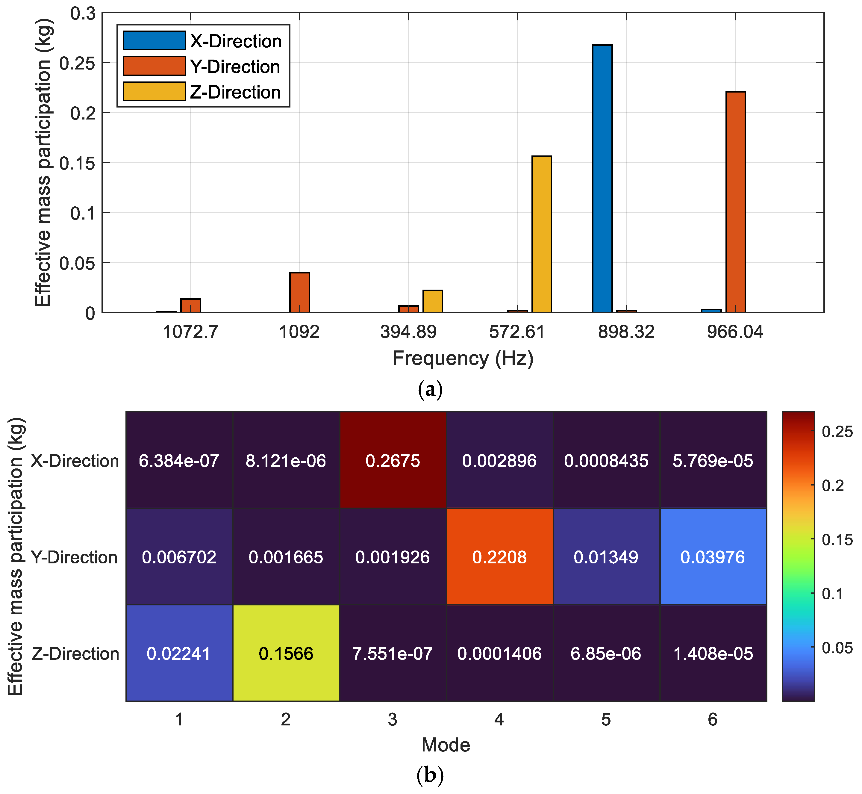
In Figure 8a, the X-direction exhibits the highest EMPF value at 1073 Hz, with a peak participation factor of 0.2675 kg, suggesting that the primary dynamic influence along this direction occurs at this resonance frequency. The Y-direction shows a peak EMPF value at 573 Hz, with substantial participation compared to other directions, with a pronounced dynamic response at this frequency. The Z-direction is relatively significant at 966 Hz, contributing more compared to other frequencies, highlighting that the Z-axis plays a noticeable role in the system dynamics at higher resonance frequencies. In Figure 8b, the X-direction at mode 2 shows the highest EMPF of 0.2675 kg, aligning with the peak at 1073 Hz observed in Figure 6a, appearing to dominate the dynamic response in the X-direction. The Y-direction at mode 4 exhibits its highest EMPF value of 0.2208 kg, consistent with the peak at 573 Hz, indicating influences of the dynamic behavior of this mode along the Y-axis. The Z-direction at mode 3 shows the highest EMPF value of 0.1566 kg, indicating that this mode is critical for oscillations in the Z-direction. The EMPF analysis at a 90° opening reveals a highly directional and mode-dependent dynamic response, with critical influences from the X, Y, and Z-directions at specific frequencies and modes.

Table 6. Boundary conditions of the CFD analysis.

Type	Inlet Mass Flow
Flow parameters	Flow vector direction: Normal to face Mass flow rate: 440 kg/s Fully developed flow: Yes
Thermodynamic parameters	Temperature type: Temperature of initial components Temperature: 293.20 K
Type	Outlet Environment Pressure
Thermodynamic parameters	Environment pressure: 101.325 kPa Temperature type: Temperature of initial components Temperature: 293.20 K

outlines the boundary conditions applied in the CFD analysis of the concentric double-flange butterfly valve system. The inlet boundary condition prescribes a defined mass flow rate directed normal to the inlet face, ensuring that the flow enters the computational domain in a fully developed state. At the outlet, an environmental pressure condition governs the fluid’s exit, maintaining thermodynamic consistency throughout the analysis.

The meshing diagram shown in Figure 9 effectively demonstrates the discretization applied to the butterfly valve system. The level of refinement indicates an effort to capture critical geometrical and physical details to ensure accurate simulation results for the CFD study. In this analysis, the fluid force at a 30° valve opening is identified as a benchmark to verify the optimal mesh size that balances accuracy and efficiency in computational simulation.

Table 7. Mesh refinement information of CFD analysis.

Level	Refinement (mm)	Fluid Force (N)
1	2.0	48,017.268
2	1.0	48,114.907
3	0.5	48,222.311
4	0.25	48,232.075

shows the computed fluid force corresponding to each refinement, with the data demonstrating the influence of mesh refinement on fluid force. As the refinement value decreases, the fluid force converges toward a specific value, indicating grid independence.

Table 8. Flow characteristic of a butterfly valve at 30°, 60°, and 90° opening positions.

30° Valve opened
60° Valve opened
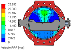
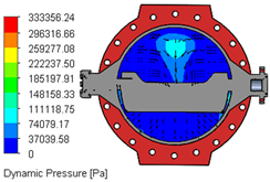
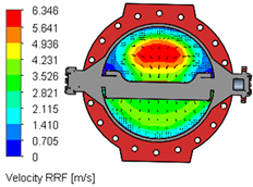
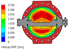
90° Valve opened

captures flow characteristics of the concentric double-flange butterfly valve when the disk transitions through opening angles of 30°, 60°, and 90°. The measurements reveal how the internal geometry of the valve is dictated by the position of the disk, altering the fluid behavior passing through the system. When the valve stands at an opening angle of 30°, the passage for the fluid remains significantly constricted. The disk occupies a large fraction of the valve cross-sectional area, forcing the fluid to accelerate through a narrow gap. In such a case, the overall low flow rate is restricted, since less fluid passes through per unit time. Simultaneously, the fluid experiences a pronounced pressure drop across the valve, as the obstruction forces change direction rapidly by generating high local velocities and substantial energy losses. At the narrow opening, regions of recirculation and vortex formation develop downstream of the disk, which enhances turbulence intensity and imposes fluctuating forces on the valve disk. As the opening angle shifts to 60°, the available flow area expands significantly. Now the fluid encounters a broader path that permits a higher flow rate compared to the 30° case. However, the disk still intrudes into the flow domain enough to cause some obstruction. The pressure drop across the valve remains noticeable but is less severe than at 30°. The fluid velocity becomes distributed over a wider region of the valve cross-section, reducing the sharpness of velocity peaks observed at lower openings. The extended recirculation zones diminish, although localized turbulence can persist around the edges of the disk and shaft. At this stage, the flow shows some asymmetry because the disk remains partially open, yet the conditions become more stable than at lower openings. At a 90° opening angle, the disk aligns almost parallel to the flow direction and leaves the valve largely unobstructed. The fluid moves with minimal interference and reaches the highest flow rate among the three positions. The pressure drop across the valve drops further as the fluid path becomes less complex and energy losses decrease.

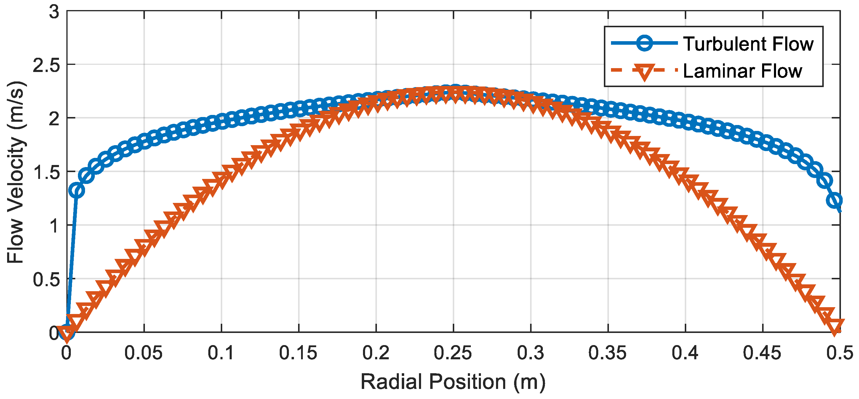
Figure 10 presents the velocity profiles for turbulent and laminar flow in a butterfly valve plotted against the radial position. The turbulent flow reflects the nature of the turbulent motion of a flatter velocity distribution near the center of the valve. The velocity drops sharply near the valve walls due to the no-slip condition and forces the flow velocity to become zero at the boundary. The flatter profile results from the mixing and energy transfer in turbulence, which reduces velocity gradients in the central region. In contrast, the laminar flow profile displays a parabolic shape typical of fully developed laminar flow. The velocity reaches its maximum at the valve’s center and declines steadily to zero at the walls due to the lack of mixing between fluid layers.

5. Conclusions

The modal behavior of a concentric double-flange butterfly valve was analyzed through FEA to evaluate its performance and dynamic characteristics. The X-direction showed the highest EMPF values at specific resonance frequencies of 1153.1 Hz and 912.21 Hz, with peak values around 0.2631 kg and 0.08161 kg, respectively. The Y-direction demonstrated moderate EMPF values, particularly at 392.06 Hz and 559.45 Hz frequencies, with significant contributions of 0.1239 kg and 0.08161 kg in specific modes. The Z-direction exhibited minimal dynamic impact, with the highest EMPF at 0.1218 kg, indicating less susceptibility to vibrations in this direction. Higher dynamic participation was observed in Mode 3 and Mode 4 across all three directions, particularly for the X and Y directions. The modes highlighted critical frequencies requiring potential damping mechanisms to mitigate resonance effects. The X-direction exhibited increased resonance sensitivity at higher frequencies, while the Y-direction suggested areas for reinforcement to minimize dynamic effects. Modes with higher mass participation factors indicate potential zones for stress concentration. Critical areas tend to experience repeated stress cycles that may contribute to fatigue. Computational Fluid Dynamics analysis examined the fluid flow behavior for valve openings set at 30°, 60°, and 90°. The analysis showed intricate flow structures marked by separation zones, recirculation areas, and variations in turbulence intensity. Lower valve openings caused notable pressure drops and created local zones with steep velocity gradients. Fully open positions lowered flow resistance and led to more stable velocity profiles. The combined use of structural and fluid dynamics analyses enables a clearer understanding of how flow-induced forces interact with structural responses. Further research will aim to include fully coupled Fluid–Structure Interaction (FSI) models and experimental validation to improve predictive accuracy and support the development of butterfly valve designs that achieve better dynamic stability and reliable performance in industrial settings. A model including elastic–plastic material behavior, particularly for dynamic analyses under impact scenarios where the valve might experience loads exceeding elastic limits, can also be explored.