Abstract
This paper introduces a novel approach by employing a Monte Carlo simulation to investigate the impact of various design parameters on the performance of two-body wave energy converters. The study uses a simplified analytical model that eliminates the need for complex simulations such as boundary elements or computational fluid dynamics methods. Instead, this model offers an efficient means of predicting and calculating converter performance output. Rigorous validation has been conducted through ANSYS AQWA simulations, affirming the accuracy of the proposed analytical model. The parametric investigation reveals new insights into design optimization. These findings serve as a valuable guide for optimizing the design of two-body point absorbers based on specific performance requirements and prevailing sea state conditions. The results show that in the early design stages, device dimensions and hydrodynamics affect performance more than the PTO’s stiffness and damping. Furthermore, for lower frequencies, adjustments to the buoy’s height emerge as a favorable strategy, whereas augmenting the buoy radius proves more advantageous for enhancing performance at higher frequencies.
1. Introduction
In the contemporary era, ocean wave energy has garnered substantial attention as an alternative, renewable power source due to its remarkable power density [1]. Although wave energy concepts date back to the late 18th century, full-scale WEC trials remain limited compared to other renewable technologies. Two main factors explain why WEC development has lagged behind solar, wind, and hydro technologies. Firstly, the multidisciplinary nature of WEC design necessitates a profound theoretical foundation [2,3,4,5,6,7,8]. Secondly, the challenges and substantial costs associated with testing full-scale prototypes in harsh sea conditions pose significant obstacles [9,10,11,12,13]. Ruehl and Bull [14] outlined a roadmap for WECs to attain full commercial viability. However, a survey of recent advancements and research in WECs [9,15] suggests that wave energy conversion technology lags behind other renewable energy methods in achieving full-scale commercial realization.
Diverse types of WECs, suitable for both near-shore and far-offshore settings, exist. The point absorber represents a simple variant, featuring a buoyant float that oscillates on the water’s surface to harness the considerable wave-induced forces. This kinetic energy is harnessed through a Power Take-Off (PTO) mechanism situated between the buoy and a fixed reference point [1]. The point absorber holds potential even in high-energy, far offshore environments, where the ocean waves carry substantial energy density [16]. This makes it a prime candidate for advancing WECs towards commercialization, given its potential for high conversion efficiency [17]. Locations with significant wave energy, like the southern coast of Australia, often exhibit extended ocean wave periods larger than 8 s [16,18]. Point absorbers are most efficient when the incoming wave frequency aligns with their resonant frequencies [17,19]. Thus, researchers have proposed adding a submerged body to the buoy of point absorbers to decrease their natural resonant frequency and enhance power capture. This submerged oscillating body reduces the resonance frequency by increasing physical dry mass and hydrodynamic added mass. The augmented system inertia results in higher captured power through relative motion between the buoy and the submerged body [19,20,21,22]. Incorporating a submerged body elevates the complexity of point absorbers [23], as various parameters impact the performance of these two-degree-of-freedom WECs. Traditional sensitivity analyses for two-body WECs rely on linear BEM [19,21,24] or computationally intensive nonlinear CFD simulations [3,24,25,26]. These studies compute detailed hydrodynamic properties for use in frequency-domain linear models [2,27]. For example, Wu, Wang, Diao, Peng and Zhang [27] derived a solution for hydrodynamic properties in a two-body WEC with heaving cylinders, performing an initial parameter study that identified design parameters linked to device resonance frequency as the main influencers of performance output. However, the model was complex and ignored viscous drag from the submerged body, leading to overestimated efficiency. It is well-established that this viscous damping drag force acting on the submerged body of a two-body WEC can reduce the absorbed power of two-body WECs by 10–30% [21]. Many other parameter and optimization studies across the literature rely on BEM simulations for hydrodynamic properties, constraining analysis as each new response calculation necessitates a fresh BEM simulation [28,29,30,31,32]. Monte Carlo, genetic algorithm, and machine learning methods require large datasets for optimization studies. Consequently, significant computational resources are required due to the need for new BEM or CFD simulations whenever the device’s geometric configuration is altered. Liu, et al. [33] present a novel quasi-zero-stiffness (QZS) device using piezoelectric buckled beams that simultaneously provides superior vibration isolation and energy harvesting compared to conventional, single-purpose systems where the analytical model was developed for numerical optimization.
This paper introduces a simplified hydrodynamic model for studying how design parameters affect wave energy performance using Monte Carlo simulations. Six Monte Carlo simulations were executed to comprehensively scrutinize the influence of diverse design parameters on the response and performance of two-body WECs. This study uniquely expresses displacement, power output, and natural frequencies as functions of sea state and device dimensions. By furnishing the Monte Carlo simulation results within this study, readers can fine-tune the design parameters of a two-body WEC to achieve desired performance outcomes within specific sea conditions.
The remainder of this paper is structured as follows: Section 2 elaborates on the analytical mathematical model, Section 3 validates the analytical mathematical model via BEM simulation, Section 4 outlines the findings of the Monte Carlo simulations, Section 5 engages in a discourse on these outcomes, and, finally, Section 6 draws conclusions from the presented study.
2. Mathematical Formulation of System Dynamics
2.1. Dynamics of Two Body Point Absorber Wave Energy Converter
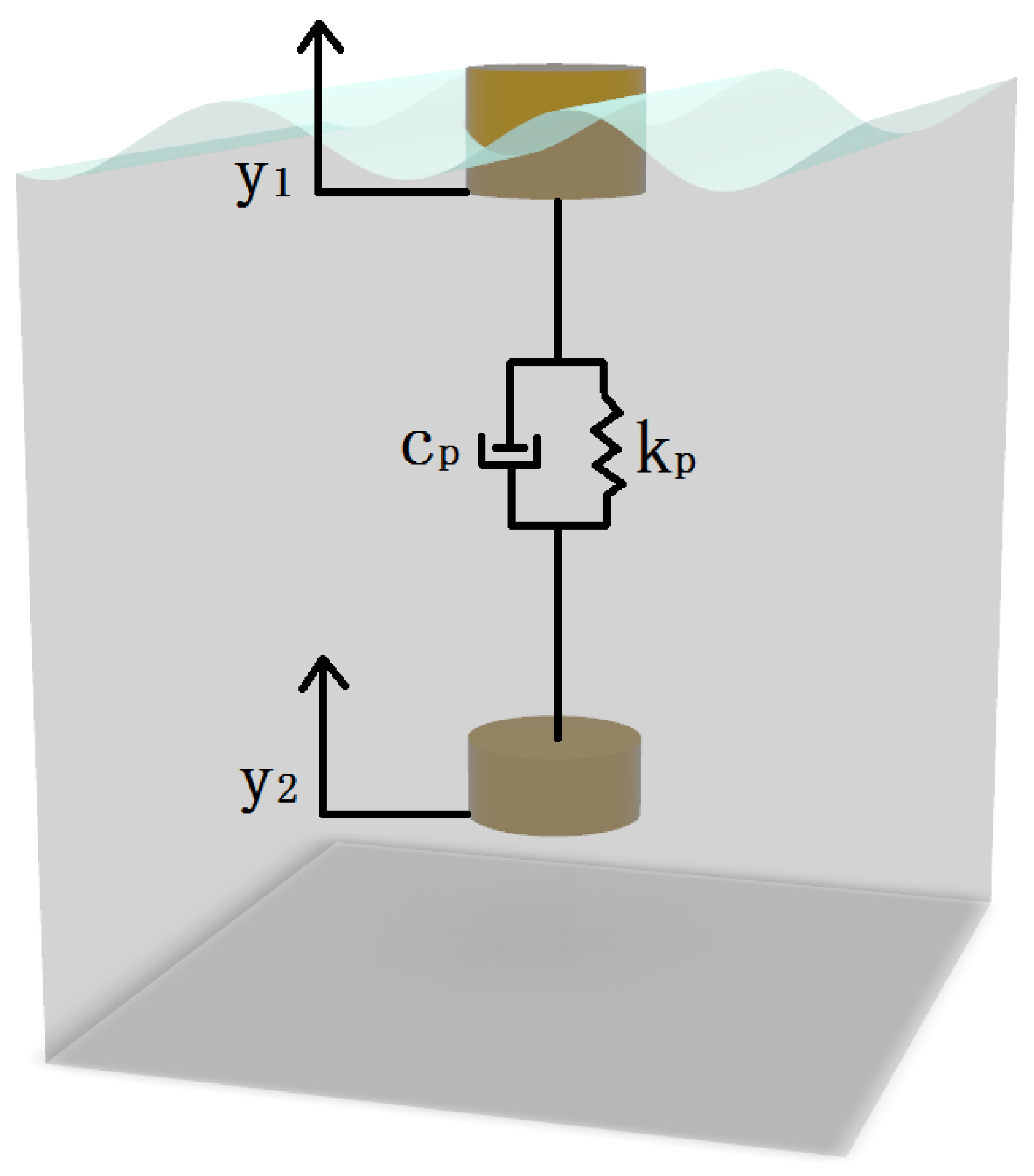
Figure 1 displays the schematic of the described WEC system. The WEC is composed of a cylindrical floating buoy, and a cylindrical submerged body connected by a linear generator. In order to simplify the model, all the forces are linearized, including the hydrodynamic and viscous damping, and PTO forces. This renders the model a two-degree-of-freedom mass-spring-damper system, with a linear PTO operating as a result of the relative movement of the buoy and the submerged body. Point absorbers primarily operate in the heave direction because wave excitation forces—and thus energy—in that direction are much greater than in others [2,27,34,35]. This study focuses solely on heave motion for wave energy conversion. In later design stages, mooring will be added to the submerged body, which may introduce surge or pitch motions that must be considered.

Figure 1.
Schematic of the studied two body WEC.
We applied Newton’s second law of motion in the two-degree-of-freedom oscillating system:
With denoting the buoy, and denoting the submerged body. and represent the displacement, velocity and acceleration of the oscillating bodies, respectively. is the total mass of an oscillating body, which is composed of both the dry mass and the hydrodynamic added mass . represents viscous drag damping, is radiation damping, and is hydrostatic stiffness—the restoring force caused by the difference between buoyancy and weight as the device oscillates. and are the linear PTO’s stiffness and damping coefficients, respectively, which are used to calculate the PTO force, Fp from the relative displacement and relative velocity between the buoy and submerged body: . is the wave excitation force. Finally, and are the hydrodynamic radiation damping and added mass interactions between the two oscillating bodies, respectively.
The total mass is composed of both the dry mass and the hydrodynamic added mass:
The purpose of this work is to develop an analytical model which can predict the response of a two-body point absorber efficiently with a low number of required parameters. The frequency domain is accurate enough to model the linear interactions of point absorbers, although the frequency domain analysis is only applicable to a linear system due to the requirement of Fourier transformation. Therefore, to reduce the complexities, one can assume that the incoming wave is regular and harmonic [3,19,28,36,37]. This presents the following set of harmonic equations in the frequency domain:
where t is time, is the complex amplitude of the displacement of the two bodies, is the complex amplitude of the wave excitation force, , is the imaginary unit and equal to square root of −1, and is the wave angular frequency. j is the phase difference in the displacement of the two bodies, while j is the phase of the wave excitation force on the two bodies.
To reduce the complexity of Equations (1) and (2), the viscous damping drag force on the buoy, can be neglected, as it has a relatively small magnitude [4,38,39], also, the hydrodynamic interactions are equal, rendering and [2,21,27]. By incorporating these assumptions into Equations (1) and (2), substituting Equations (4)–(7) into Equations (1) and (2), and conducting some algebraic manipulations, the following equations representing the amplitude of the harmonic motions can be shown:
2.2. Hydrodynamic Analysis and Parameter Reduction
This section defines the coefficients in Equations (8) and (9) to reduce the number of required variables.
The buoyancy force exerted on the bodies in still water must be equal to their dry weights to achieve neutral buoyancy, resulting in a dry mass equal to the weight of the displaced volume of water:
represents the volume of displaced water and is the draft volume of the oscillating bodies. is the density of water. The dry mass can be expressed as:
where represents the radius of the buoy or submerged body, and is either the draft of the buoy or the height of the submerged body. In this study, the radius and height of both bodies are assumed equal to reduce the number of parameters in the Monte Carlo simulations. Different dimensions between the buoy and submerged body may alter hydrodynamic interactions, particularly those affecting resonance frequencies. Such refinements may be included in future, detailed design optimizations after the main parameters are finalized using this study. The intent of this work is to illustrate a method for conducting high-level optimization using Monte Carlo simulations.
The buoy is placed in two mediums, air and water, indicating that its displacement during oscillation will create a difference between the buoyancy force and its weight. This generates a spring force effect known as the hydrostatic force. The hydrostatic stiffness is represented as:
where is the gravitational acceleration.
This work uses hydrodynamic coefficients derived by Zheng et al. [3], who applied separation of variables and eigenfunction expansion for a two-body point absorber with cylindrical components. The work presented in this paper is based on [2,27] where it is assumed that the draft of the buoy in calm waters is equal to the height of the submerged body, both the cylindrical buoy and submerged body have the same radius, the distance between the buoy and the submerged body is set to ( is the sea depth), and that the fluid is considered to be incompressible, irrotational, and inviscid under the linear potential theory. Wu, Wang, Diao, Peng and Zhang [27] also derived the hydrodynamic coefficients for the same setup of point absorbers and validated this method using the results in [2].
Zheng, Shen, You, Wu and Rong [2] present an analytical investigation into the hydrodynamic properties of two coaxial, vertical, truncated cylinders interacting with linear water waves, focusing on wave forces and coefficients for heave, sway, and roll motions. The authors employ a method of separation of variables and matched eigenfunction expansion across three fluid subdomains to derive analytical expressions for the radiated and diffracted potentials. To validate the model, the study confirms that wave forces from two methods match, and the added mass and damping matrices are symmetrical. Using this verified approach, the authors calculate hydrodynamic properties and investigate their sensitivity to changes in the cylinders’ radii, providing useful data for the design of such multi-body floating structures in ocean engineering. The data from [2] will be used in this section.
Exponential and rational fitting models were used in MATLAB 2023b. The exp2 fitting function fits data as the sum of two exponential terms and the rat55 function fits a rational model, which is the ratio of two polynomials. Specifically, it uses 5th-degree polynomials in both the numerator and denominator to fit the data, allowing more efficient computation than using full analytical or BEM/CFD models. It should be noted that A is the wave height, and k is the wave number, which is calculated from the following dispersion relation:
Point absorbers are suitable for areas with large ocean depth and high energy density, where kh >> 1, allowing the wave number to be approximated as follows:
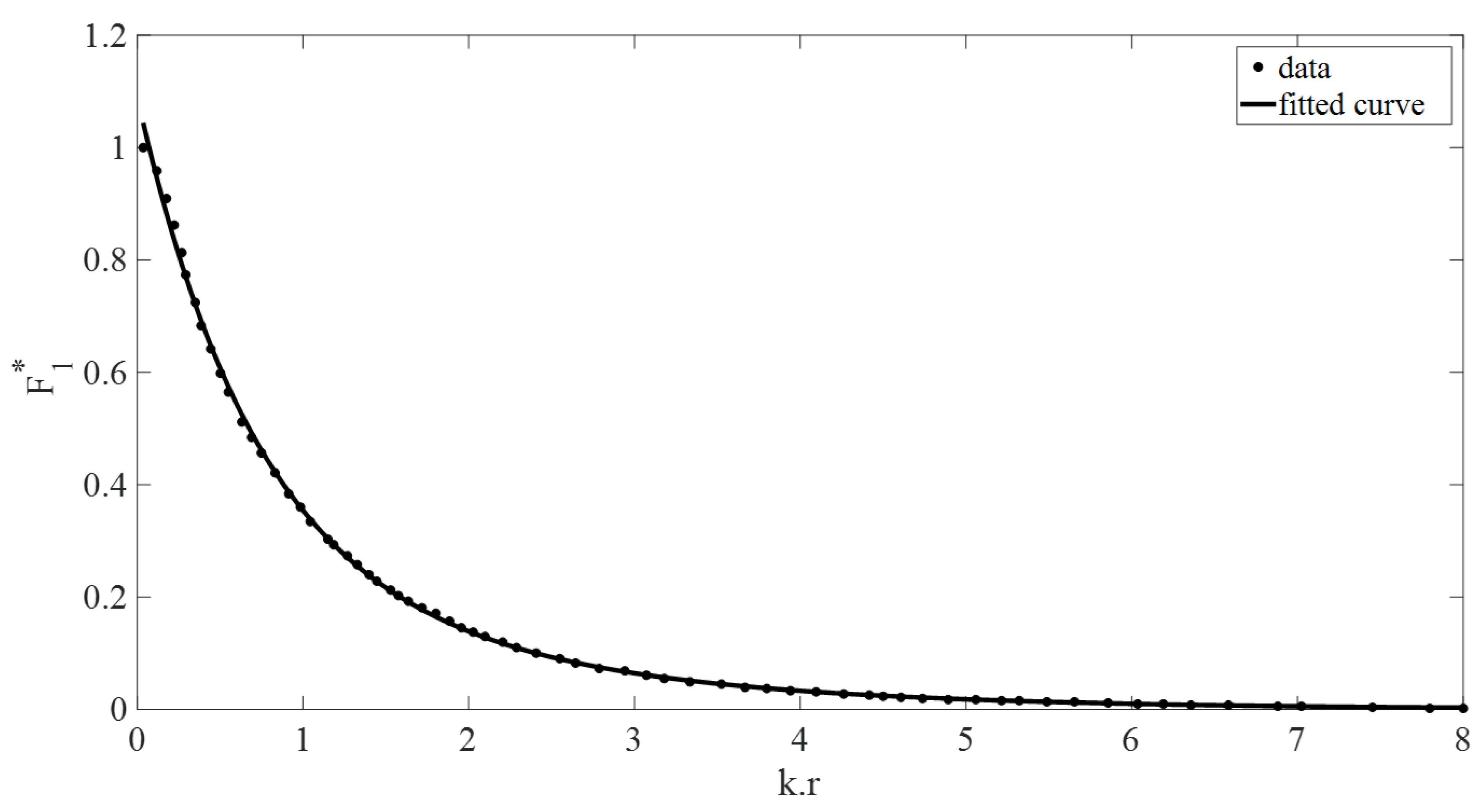
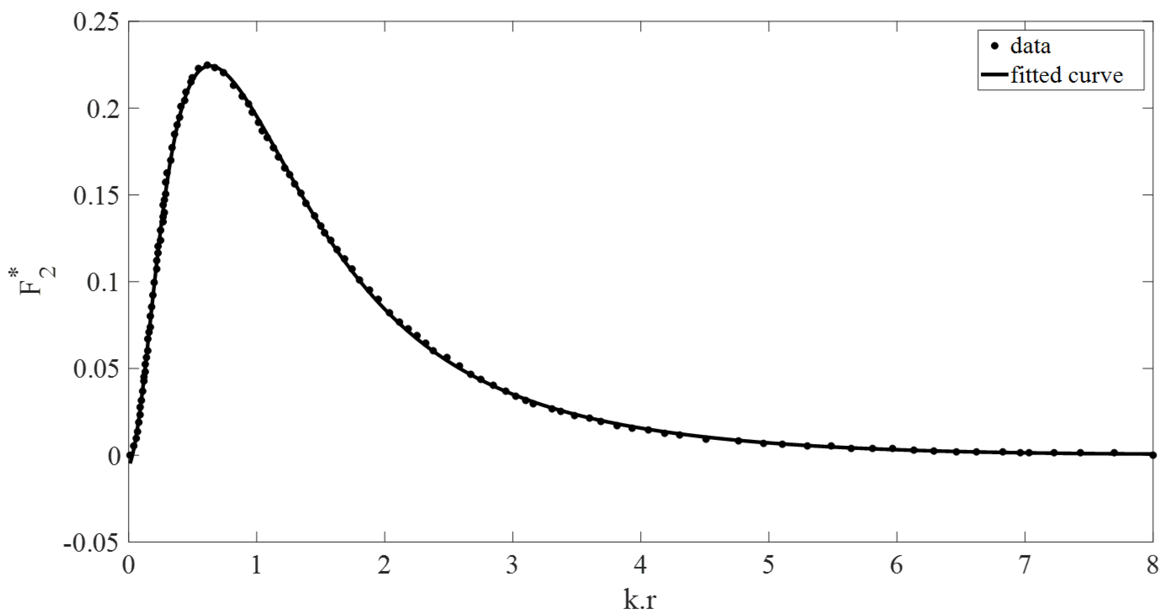
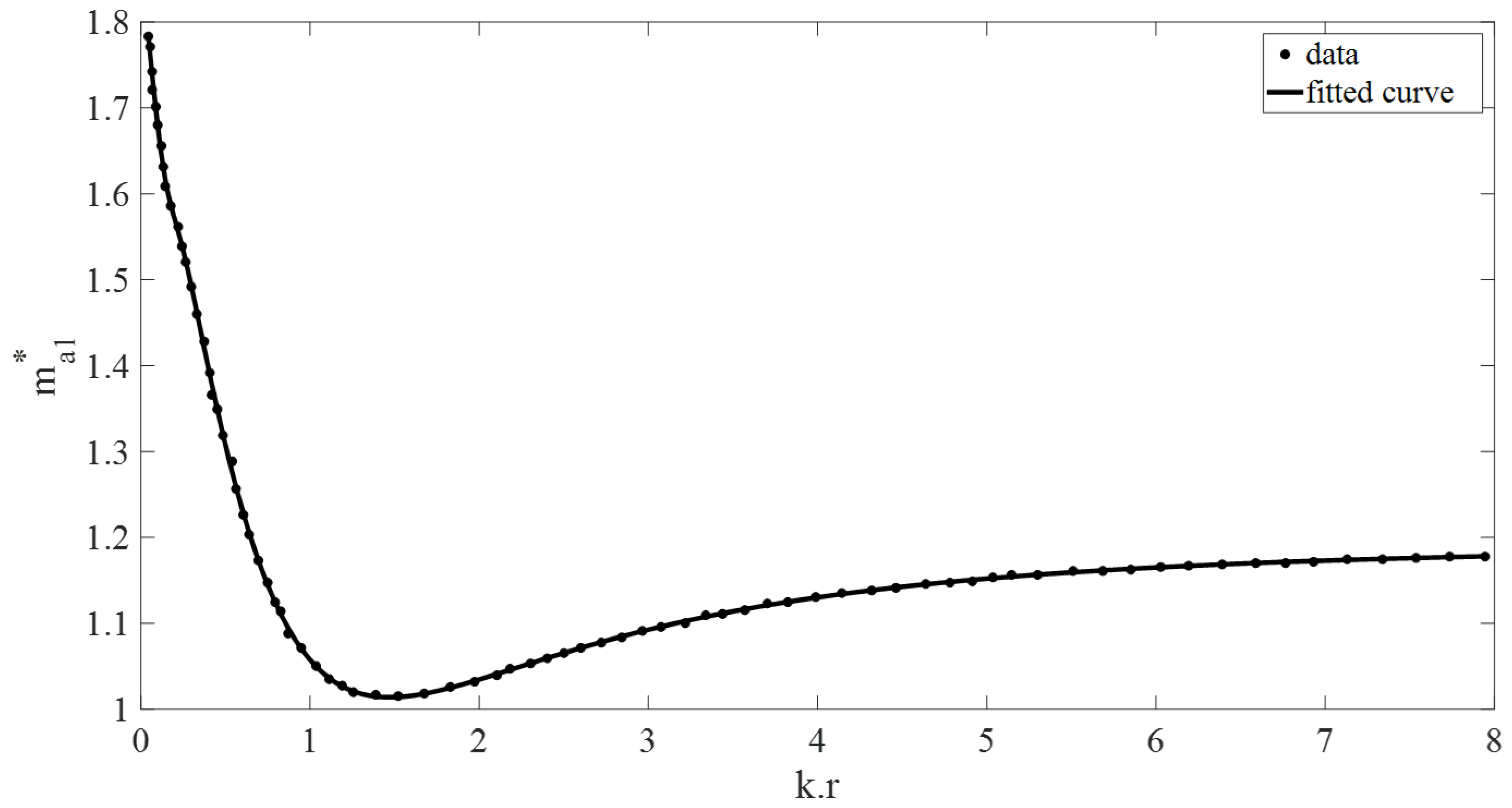
As seen from the figures below (Figure 2, Figure 3, Figure 4, Figure 5, Figure 6, Figure 7, Figure 8 and Figure 9), the fitting curves of the non-dimensional hydrodynamic coefficients accurately represent the adopted analytical solution from the past literature. Additionally, their fitting curves as a function of , or for large sea depths, as a function of are calculated and shown in Appendix A.
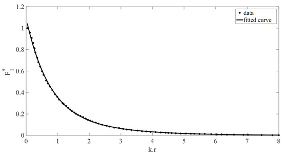
Figure 2.
Non-dimensional buoy wave excitation force vs. (kr). The dotted data used is from [2].
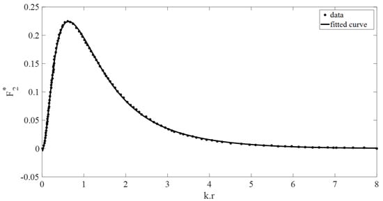
Figure 3.
Non-dimensional submerged body wave excitation force vs. (kr). The dotted data used is from [2].
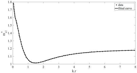
Figure 4.
Non-dimensional buoy added mass vs. (kr). The dotted data used is from [2].
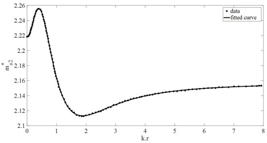
Figure 5.
Non-dimensional submerged body added mass vs. (kr). The dotted data used is from [2].
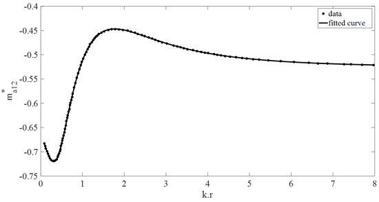
Figure 6.
Non-dimensional interaction added mass vs. (kr). The dotted data used is from [2].
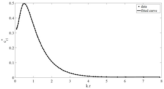
Figure 7.
Non-dimensional buoy radiation damping coefficient vs. (kr). The dotted data used is from [2].
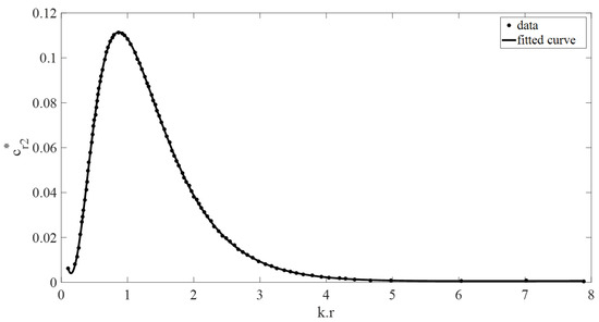
Figure 8.
Non-dimensional submerged body radiation damping coefficient vs. (kr). The dotted data used is from [2].
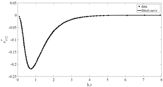
Figure 9.
Non-dimensional interaction radiation damping coefficient vs. (kr). The dotted data used is from [2].
The non-dimensional wave excitation forces on the buoy and the submerged body are, respectively, given by:
The non-dimensional added masses of the buoy and submerged body are, respectively:
The non-dimensional radiation damping coefficients of the buoy and submerged body are, respectively:
The non-dimensional interaction added mass and radiation damping coefficients of the buoy and submerged body are, respectively:
Although the viscous damping drag force acting on the buoy is small and negligible, the viscous damping drag force acting on the submerged body cannot be neglected as it is proven to have a considerable impact on the absorbed power [21,28]. The viscous damping drag force is a nonlinear force which acts in the opposite direction to that of the motion of the device, and is given by the Morison drag force equation:
is the dimensionless viscous damping coefficient. To linearize the equations of the system for the convenience of the solution, Siow, et al. [40] linearized the Morison drag force as the following:
where is the maximum heaving velocity of the submerged body and . This linearization renders the viscous damping drag force to be a function of geometric parameters. Since this paper is focused on the cylindrical oscillating bodies, the non-dimensional viscous damping drag coefficient can be set equal to 1 [24,41]. The non-dimensional viscous damping drag coefficient is typically a function of the radius to height ratio, however, a nominal value of 1 was chosen as the radius to height ratio in order to reduce the complexity of the numerical model.
2.3. Method of Solution
With all hydrodynamic parameters defined, this section presents the method to solve for the response and absorbed power for a two-body point absorber analytically without the need to conduct the hydrodynamic BEM/CFD simulations.
The response for a given sea state—defined by wave height and frequency—can be calculated by solving Equations (8) and (9), or alternatively, one can conduct the Fourier transform of Equations (1) and (2) and solve for the response for a range of frequencies or wave heights via a loop:
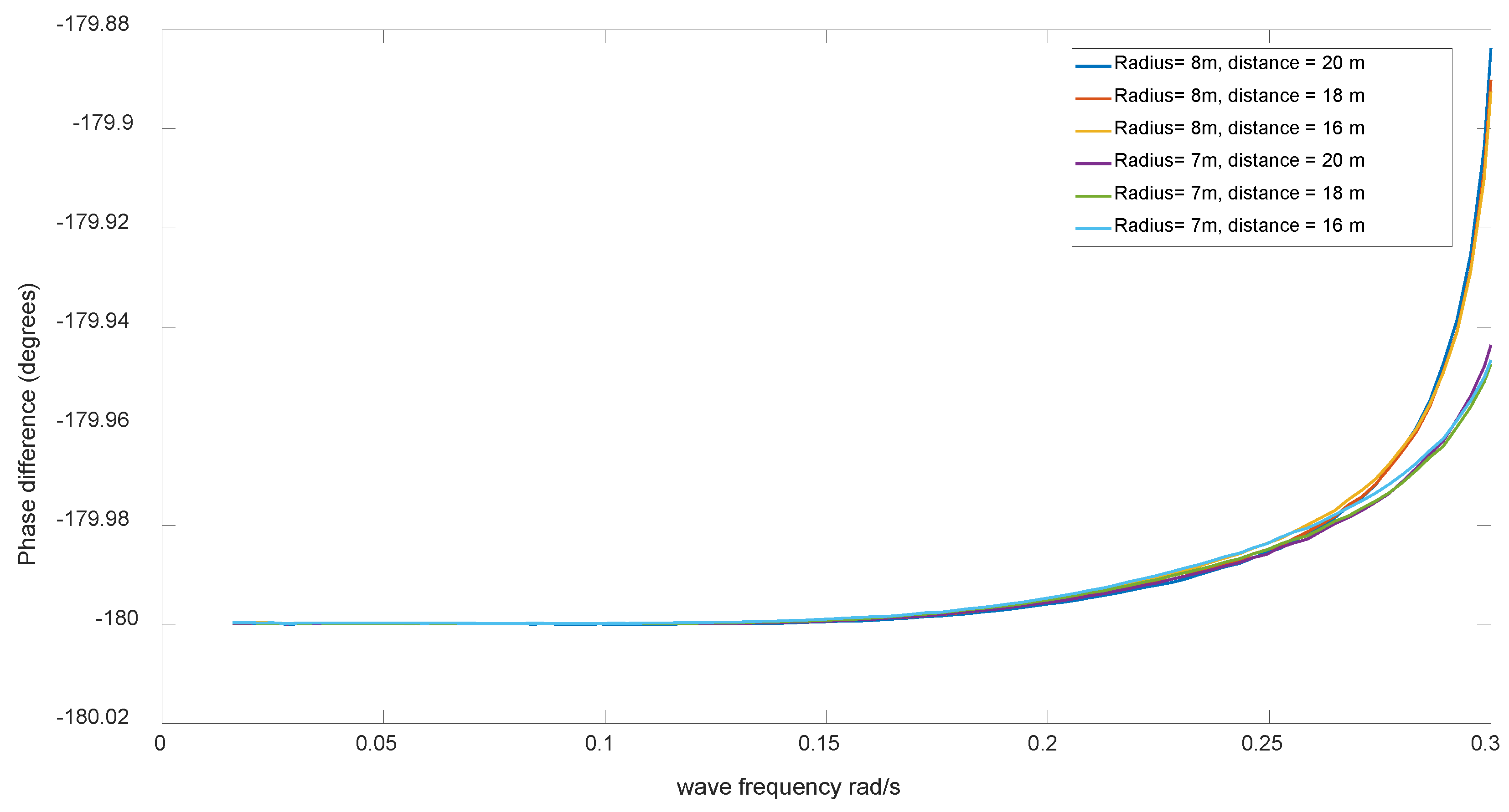
To calculate response and power, the remaining required outputs are the phases of the wave excitation forces. However, for a two-body WEC, the phase difference in the wave excitation force between the buoy and the submerged body is around −180 degrees. As can be seen in Figure 10 below, the phase difference for the wave excitation force between the buoy and the submerged body is plotted for different radiuses of the buoy and the submerged body and for different distances between the buoy and the submerged body. The results are based on the simulations from ANSYS AQWA 2019. Nonlinear resonance dynamics [42,43] are assumed negligible in this study.
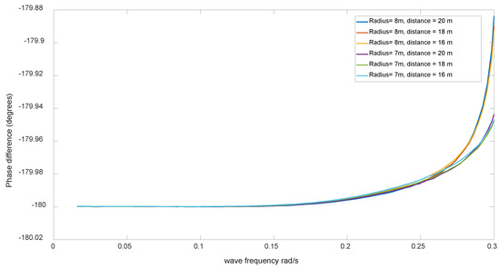
Figure 10.
The phase difference between the buoy and the submerged body for different radius of the buoy and the submerged body and for different distances between the buoy and the submerged body.
The linear PTO, placed between the two bodies, generates electricity from their relative motion. After calculating the heave displacements of the buoy and the submerged body, the average absorbed power by the linear generator PTO can be calculated as follows:
where is the period of the wave in seconds. After the geometric parameters of and and the sea state parameters of , and are provided, all the coefficients in Equations (9)–(22) can be calculated.
As for the linear PTO coefficients, either and constant values are used for control or impedance matching is applied. Impedance matching is considered a passive control algorithm [19], where the linear PTO electrical stiffness and damping coefficients are equal to the external hydrodynamic stiffness and damping coefficients. Also, one can implement varying optimal PTO stiffness and damping coefficients as derived in [20] and given by:
Impedance matching provides a passive control algorithm which predicts the response under more realistically controlled conditions. Impedance matching reduces the number of variables by linking PTO stiffness and damping to the device’s hydrodynamic properties. The device’s hydrodynamic parameters are functions of the geometry and sea state parameters. Reactive control strategies, such as reactive tuning or model predictive control, can yield better power output than the passive approach used in this study. However, the passive control strategy was selected in order to avoid nonlinearities in the mathematical model and for maintaining a high computational efficiency of the mathematical model.
One of the most important performance aspects of point absorbers is their operation around the resonance, as their power capture considerably increases when the point absorbers are resonating at the incoming ocean wave frequency [17,19]. Throughout the literature [19,21,28,29], the natural resonant frequency of a two-body system is calculated by assuming that it is a one-degree mass spring undamped oscillator, ignoring the hydrodynamic interactions between the two oscillating cylinders [24]
If one applies impedance matching, by substituting Equations (12) and (28) into Equation (29), the fundamental natural resonant frequency with impedance matching becomes:
In reality, two-body point absorbers are a two-degree of freedom system with two distinct natural resonant frequencies [44]. Neglecting the hydrodynamic interactions between the two oscillating cylinders, and assuming the system is a two-body undamped mass-spring system, the first and second resonating frequencies are calculated from the Eigen equation of Equations (7) and (8) which is given by:
For the convenience of the reader, the first and second natural frequencies without the impedance matching ( and ), and the first and second natural frequencies with impedance matching ( and ) are presented in Appendix B.
3. Validation
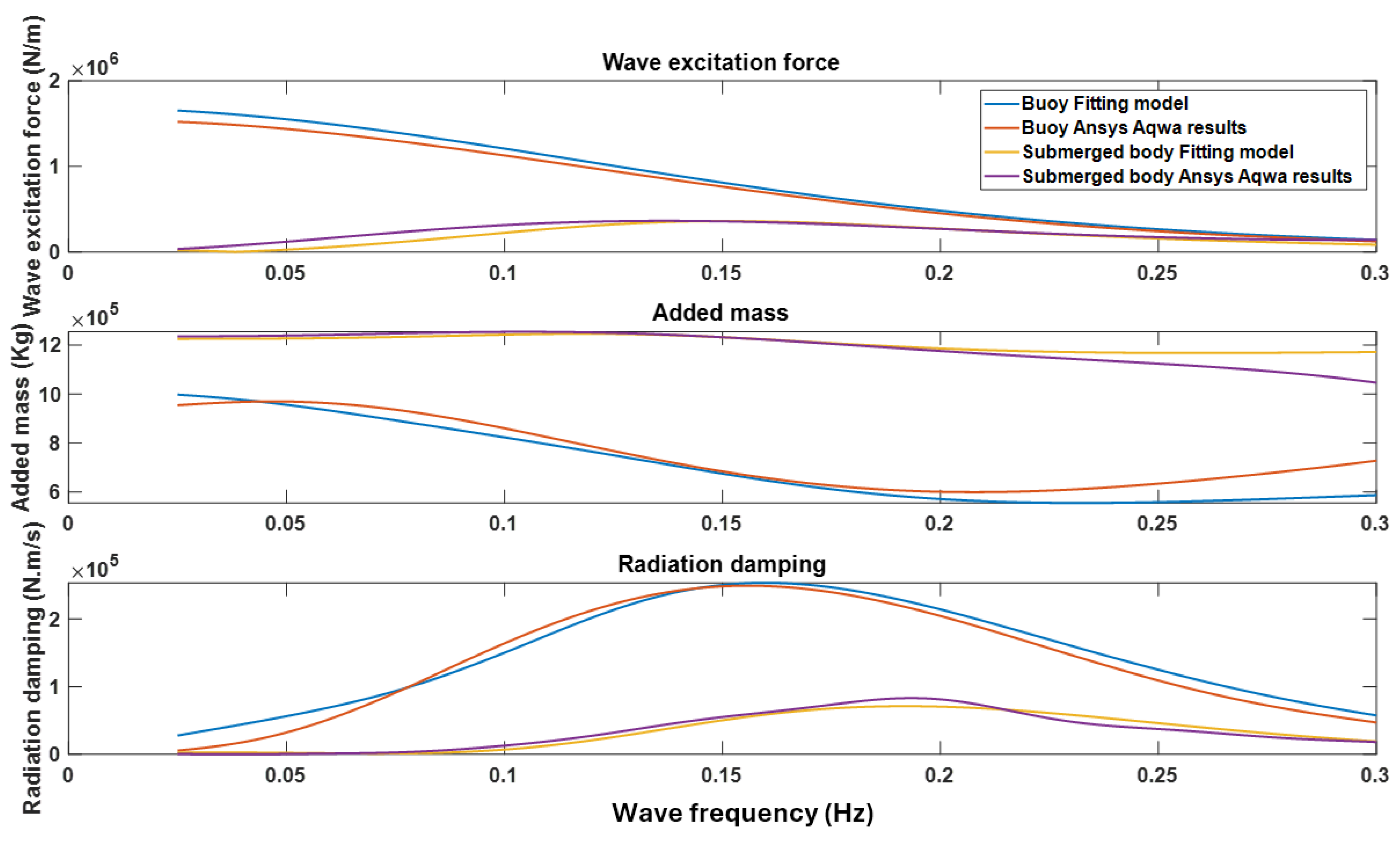
The analytical model is validated against simulations using ANSYS AQWA boundary element analysis software [23,45] The primary difference between the two models lies in how the hydrodynamic coefficients are derived—either by separation of variables and eigenfunction expansion [3] or by numerical simulation. ANSYS AQWA is boundary element analysis software that solves hydrodynamic equations around the oscillating bodies. ANSYS AQWA was extensively used throughout the literature and its results have been verified by experimental results [43]. The two-body point absorber—comprising a cylindrical buoy and submerged body—was simulated in ANSYS AQWA. The incoming wave was meshed, as shown in Figure 11. Table 1 lists the parameters used in the analytical model. A mesh sensitivity study was conducted to ensure result convergence. Hydrodynamic coefficients from ANSYS AQWA were compared with those from the analytical curve-fit model. The results are shown in Figure 12.
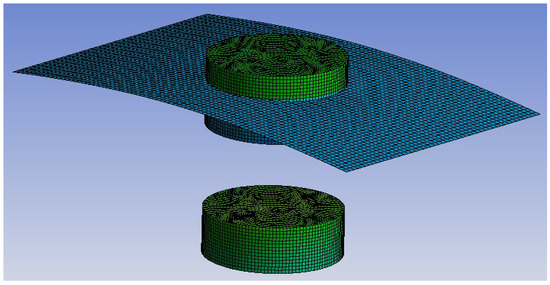
Figure 11.
Two-body point absorber mesh model in ANSYS AQWA.

Table 1.
Parameters of the model for validation.
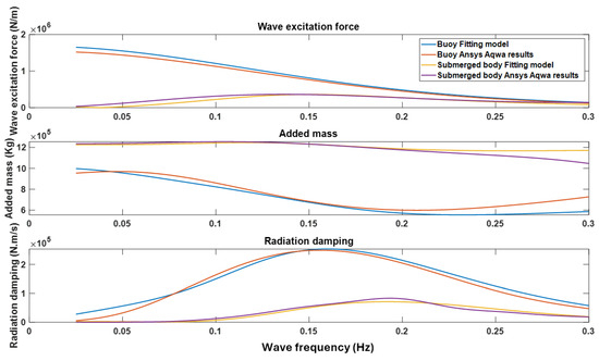
Figure 12.
The hydrodynamic coefficients from the curve fit analytical model used in this work vs. ANSYS AQWA simulation results. Wave excitation force (top), added mass (middle), and radiation damping (bottom).
Figure 12 shows close agreement between the curve-fit model and ANSYS AQWA simulations. Minor differences between the models arise from assumptions in [3] and slight variations in the fitted curves (Equations (A1)–(A8); Figure 2, Figure 3, Figure 4, Figure 5, Figure 6, Figure 7, Figure 8 and Figure 9).
Based on linear potential flow theory, the curve-fit model accurately predicts the response and absorbed power of point absorbers, supporting both design and optimization.
4. Sensitivity Analysis Using Monte Carlo Simulation
The curve-fit model offers two main advantages: it quickly computes response and absorbed power without time-consuming BEM simulations, and it helps estimate the required dimensions of a two-body WEC for a specific sea state. The second advantage is the ability to perform optimization and sensitivity analysis for two-body WECs efficiently. Traditionally, parameter analysis relied on BEM simulations for each case, which is time-consuming and limits the use of some optimization algorithms due to changing hydrodynamic properties. The curve-fit model enables designers to use optimization tools like genetic algorithms or Monte Carlo simulations to better understand two-body WEC hydrodynamics. This section presents a sensitivity analysis using Monte Carlo simulations to examine how design parameters affect two-body WEC performance. This work is part of a project aimed at designing and optimizing a wave energy converter for Australia [9,15,17,27], therefore a wave frequency of 0.1–0.13 Hz will be targeted. The simulations will study a frequency band between 0 and 0.3 Hz, but the objective of the design is to excite the device at the resonant frequency of 0.1–0.13 Hz and ensure that the maximum power absorption occurs at the frequency. The wave height is taken as 1 m.
Monte Carlo simulation is a statistical method used to study the sensitivity of design parameters to system performance [46,47,48]. As mentioned earlier, the resonant frequency of 0.1–0.13 Hz is targeted and the radius and height values of this device are used as mean values. The radius r and height h are then randomized and normally distributed with a 30% standard deviation around the mean values. The excitation frequencies studied under regular waves will be uniformly distributed between 0 and 0.3 Hz. Section 2 demonstrated that the response of a two-body point absorber can be calculated given the sea state parameters and two design parameters, and . Since the sea state is defined, the design parameters will be randomized with a 30% standard deviation around their mean values in this Monte Carlo simulation, to study their effect on device performance.
In all Monte Carlo simulations, in Equation (24), represents the maximum heaving velocity of the submerged body.
The Monte Carlo simulations are applied to study the effects of , , , and on the response and power conversion performance. Table 2 below illustrates the parameters for all the Monte Carlo simulations.
Table 2.
The Monte Carlo simulation parameters.
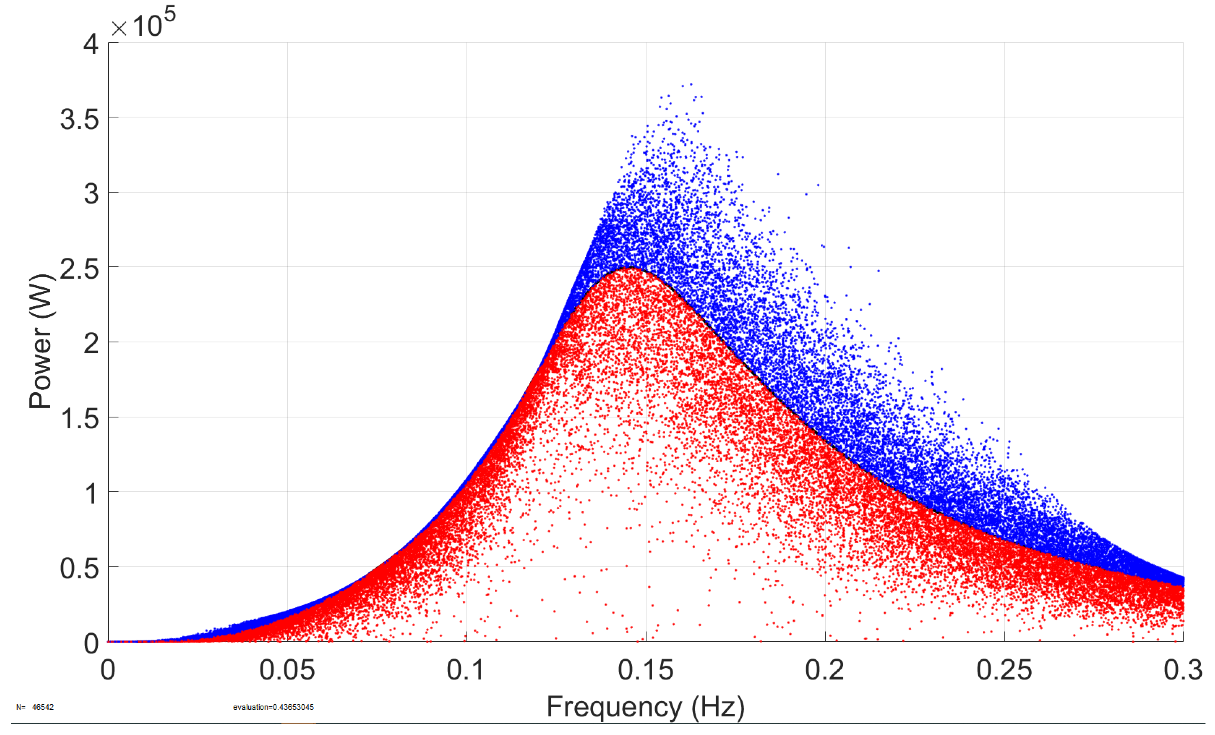
Simulations 1 and 2 examine how varying the buoy radius (r), randomized around a 7 m mean, affects power absorption. Simulation 1 will have the constant PTO stiffness and damping coefficients for all the Monte Carlo simulation runs, while Simulation 2 listed in Table 2 will utilize the varying optimal PTO coefficients derived by [21]. Simulations 3 and 4 will study the effect of the draft of the buoy on the power absorption of the system, with randomly varying the parameter around its mean value of 3.5 m. Simulation 3 will have the constant PTO stiffness and damping coefficients for all the Monte Carlo simulation runs, while Simulation 4 will utilize the varying optimal PTO coefficients derived by [21]. Simulation 5 explores the effect of varying kp around its mean value of 2,428,840 N/m on power absorption, while keeping all other parameters, including cp, constant. It should be noted that this value of is the value which results in the highest power absorption around the desired frequency range, hence it is the value that results in the resonance of the system in that range. Simulation 6 investigates how varying cp around its mean value of 4,745,450 N·s/m affects power absorption, with all other parameters held constant. This value of yields the highest power absorption around the desired frequency range. Each simulation was run for 40,000–45,000 iterations to reveal performance trends. As shown in Figure 13 and Figure 14, one should note that the black line is the absorbed power with the mean parameter values, and the colored dots represent the absorbed power values with the randomized parameter values. The blue dots represent the absorbed power values larger than those with the mean parameter values. The red dots represent the opposite, i.e., absorbed power values lower than those with the mean parameters. This section will showcase the results, and they will be analyzed and discussed in the section below.
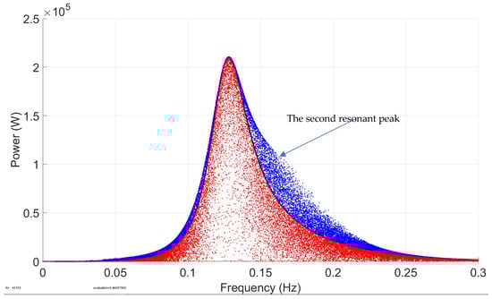
Figure 13.
Simulation 1 results—the power output of the system when r is randomized with a 30% standard deviation around the mean value, with the constant PTO stiffness and damping coefficients.
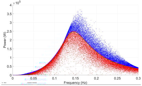
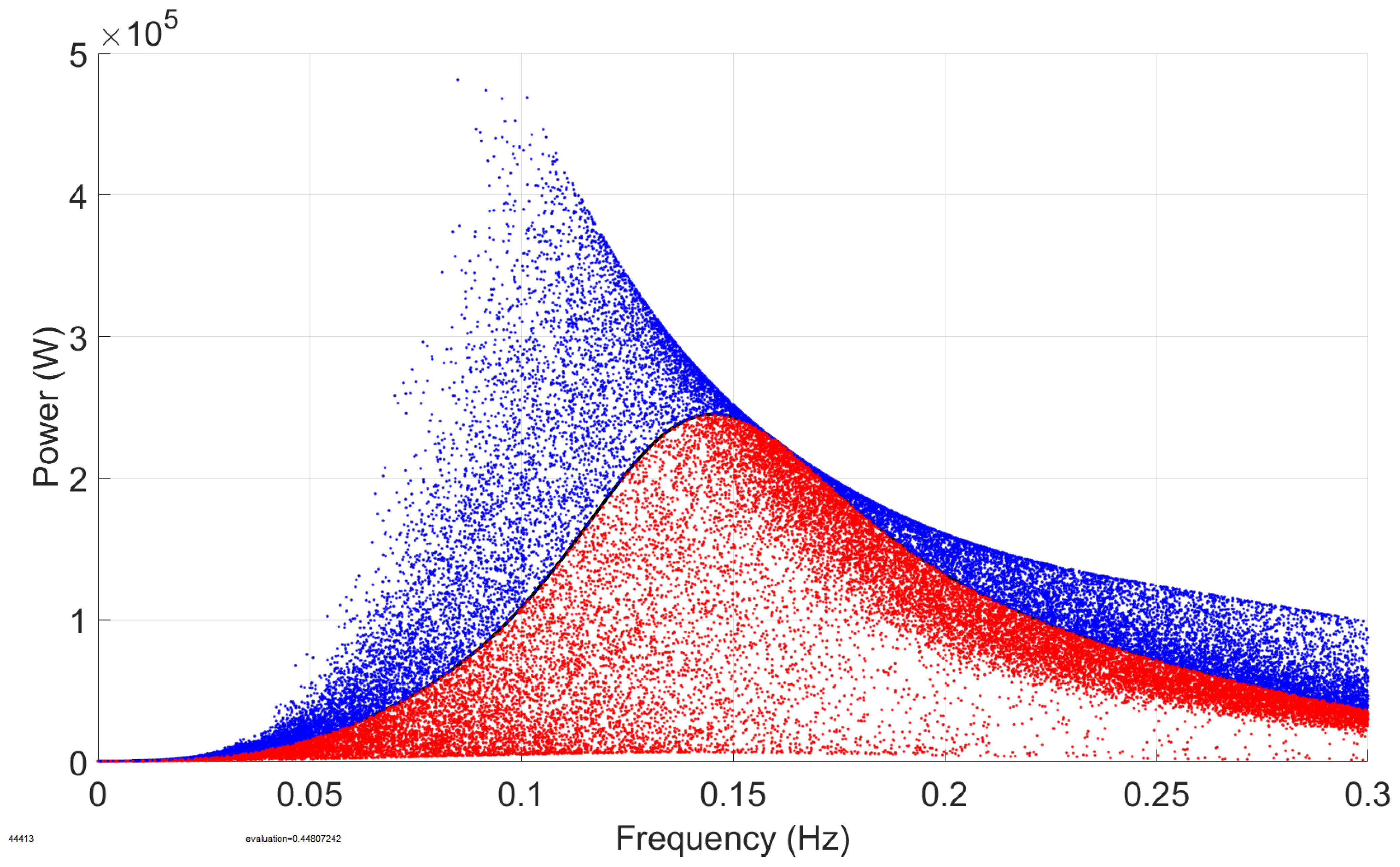
Figure 14.
Simulation 2 results—the power output of the system when r is randomized with 30% standard deviation around the mean value, with varying optimal PTO stiffness and damping coefficients.
Figure 13 and Figure 14 showcase the effects of randomizing with a 30% standard deviation around its mean chosen value. In Figure 13 the PTO stiffness and damping coefficients are assumed to be constant, while in Figure 14 the varying optimal stiffness and damping coefficients were used. With the constant PTO stiffness and damping coefficients, changing has little impact on system performance at the resonant frequency. It can also be observed that the second resonant absorbed power peak occurs between 0.15 and 0.2 Hz. In its mean chosen parameter values, the system mainly presents a single degree of freedom buoy dynamics with a single resonant peak. When the buoy radius changes, the hydrodynamic interaction between the buoy and the submerged body increases. The system then exhibits two-degree-of-freedom dynamics involving both the buoy and the submerged body with two resonant peaks. The random Monte Carlo (MC) simulation data points of the absorbed power have a large spread. When the optimal PTO stiffness and damping coefficients are varied in Simulation 2, is randomly varied by 30% around its mean value. It is seen that the radius r has an effect on both the absorbed power and the resonant frequency, specifically on the right-hand side of the curve peak. The results will be further discussed in Section 5 below. Figure 14 shows that both the random and mean peak absorbed power values are slightly higher than those in Figure 13 in the case with the constant PTO stiffness and damping coefficients. In its mean chosen parameter values, Figure 13 shows the absorbed power at the peak frequency of 0.125 Hz is 2.1 × 10⁵ W while Figure 14 shows that at the peak frequency of 0.14 Hz is 2.5 × 10⁵ W. In Figure 14, the mean PTO stiffness (kp) is higher, while the damping (cp) is lower compared to Figure 13. The spread of random absorbed power values in Figure 14 is larger than in Figure 13. Figure 14 shows that when r is randomized by ±30%, absorbed power can reach up to 3.75 × 10⁵ W with optimal PTO coefficients.
Figure 15 and Figure 16 showcase the effects of the buoy draft h on the average absorbed power by randomizing the buoy draft with a 30% standard deviation around its chosen mean value. In Figure 15, the PTO stiffness and damping coefficients are set to be constant, while in Figure 16, the varying optimal PTO stiffness and damping coefficients are utilized. The trends and effects were similar in both cases, as applying the optimal PTO stiffness and damping coefficients did not change much in the peak value of the absorbed power curve in the mean chosen parameters. Randomizing the buoy draft had an effect on both the average absorbed power and the resonant frequency. The absorbed power seemed to increase with the decrease in the resonant frequency and decrease with the increase in the resonant frequency. Also, it is shown that both the random and mean peak absorbed power values in Figure 16 are inconsiderably larger than those in Figure 15 in the case with the constant PTO stiffness and damping coefficients.
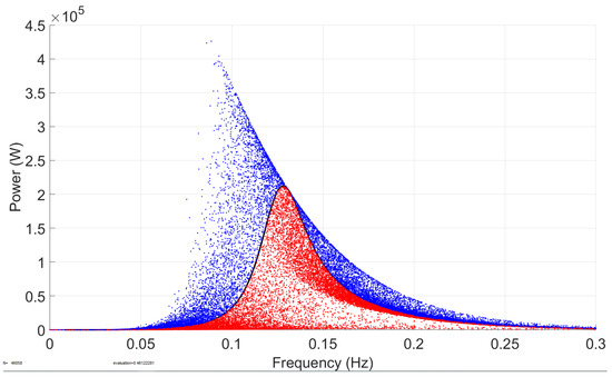
Figure 15.
Simulation 3 results—the power output of the system when the buoy draft h is randomized with 30% standard deviation around its mean value, with the constant PTO stiffness and damping coefficients.

Figure 16.
Simulation 4 results—the power output of the system when the buoy draft h is randomized with 30% standard deviation around its mean value, with the varying optimal PTO stiffness and damping coefficients.
The effect of the PTO stiffness coefficient on the average absorbed power is shown in Figure 17, and the effect of the PTO damping coefficient on the average absorbed power is shown in Figure 18. It is seen from the Monte Carlo simulation results in Simulations 5 and 6 that both the PTO damping coefficient and the PTO stiffness coefficient have a small effect on the average absorbed power output value and resonant frequency.
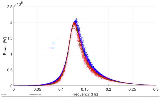
Figure 17.
Simulation 5 results—the power output of the system when kp is randomized with a 30% standard deviation around its mean value while the other parameters are not changed.
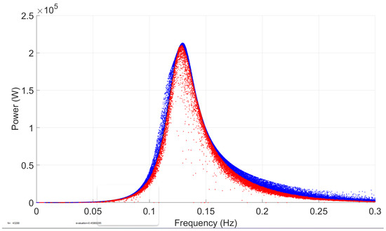
Figure 18.
Simulation 6 results—the power output of the system when cp is randomized with 30% standard deviation around its mean value, while the other parameters are not changed.
It is seen from Figure 13, Figure 14, Figure 15, Figure 16, Figure 17 and Figure 18 that the wave height h has the largest effect on the peak power output value and resonant frequency in the low frequency range (lower than the fundamental resonant frequency). The buoy radius has the second largest effect on the peak power output value and resonant frequency in the high frequency (higher than the fundamental resonant frequency). The PTO damping coefficient and the PTO stiffness coefficient have the least effect on the peak power output value and resonant frequency among all the simulations.
5. Discussions
As mentioned earlier, the system dynamic model assumes that the draft of the buoy is equal to the height of the submerged body. This assumption is acceptable given the purpose of this work which is to present a simplified analytical solution with the simplified hydrodynamic analytical model and simplified/linearized viscous damping drag force calculations for two-body WECs. The calculation of the response in the design process is used to estimate the dimensions of the WEC for a specific ocean site. This assumption is consistent with two-body point absorber configurations tested in wave tanks [49]. This model also enables sensitivity and optimization studies involving changing design parameters. Usually, changing the design parameters related to the dimensions of WECs requires a new BEM or CFD simulation, which is time-consuming. This work demonstrated the ability to conduct the Monte Carlo sensitivity analysis for two-body WECs with 40,000–45,000 runs in each simulation. Traditional BEM methods made Monte Carlo simulations impractical for two-body WECs due to high computational cost.
As for the Monte Carlo simulations, it is observed from Figure 14 and Figure 16 in Section 4 that the optimal PTO parameters (stiffness and damping coefficients) increases the bandwidth much more than increases the maximum absorbed power, which is verified by [21]. This is partly because the chosen constant PTO parameters bring the system close to resonance, where power absorption is highest. Figure 13 and Figure 14 demonstrate the effect of the buoy and submerged body radius r on the average absorbed power in Monte Carlo Simulations 1 and 2. It is seen that the power is greatly affected in the case of the optimal PTO parameters, specifically past the resonance point. This result is expected since altering r greatly affects the system’s inertia and excitation forces of the system. Many parameters—such as dry and added mass, hydrostatic stiffness, and wave excitation forces—depend on r2, though other factors also influence performance. This indicates that absorbed power is highly sensitive to changes in buoy radius. The results agree with those of some of the previous parameter studies [20,28]. Changes in buoy radius had minimal impact on absorbed power before the resonance frequency. This is due to the fact that increasing the buoy radius results in an increase in both the dry and the hydrodynamic added mass, but also increases the hydrostatic stiffness of the device, which cancels the advantages gained with regard to decreasing the resonance frequency out of the increased masses. Figure 7, Figure 8 and Figure 9 show that radiation damping is large at low frequencies and approaches zero as the wave frequency increases. This also explains why there was no meaningful increase in the absorbed power at lower frequencies. It is well known that increasing buoy radius raises dry and added masses and excitation forces. The Monte Carlo analysis further clarifies how these changes affect WEC performance, as discussed below. The increase in mass inertia due to larger buoy radius outweighed the impact of increased viscous damping at higher frequencies. The opposite trend was shown at lower frequencies. This can be specifically seen in Simulation 2, where the buoy radius has a substantial effect on both the absorbed power and the resonance frequency of the system. At frequencies larger than 0.12 Hz, with the varying optimal PTO coefficients, the effect of increasing the mass inertia through increasing the buoy radius overtook that of increasing the radiation and viscous damping drag forces, which has produced more power.
The peak of the absorbed power is much larger for the case of varying optimal PTO coefficients in Simulation 2 than that for the case of constant PTO coefficients in Simulation 1. This occurs because varying the optimal PTO coefficients brings the system into impedance matching. When r is randomized while PTO coefficients remain fixed (Simulation 1, Figure 13). Changing the buoy radius is not only affecting the geometric and hydrodynamic parameters of the device but also changing the PTO stiffness and damping coefficients to further tune the hydrodynamic properties of the system. The effect of the PTO stiffness and damping coefficients can be most seen around the resonant frequency where the velocities of the oscillating bodies are at a maximum.
If we randomize while keeping the PTO coefficients unchanged in Monte Carlo Simulation 1 as shown in Figure 13, we can see that the buoy radius does not have an effect on the resonant frequency. Another resonance frequency appears between 0.15 Hz and 0.2 Hz. For a two degrees of freedom system, the absorbed power curve of the two-body point absorber of two distinct resonant frequencies and two absorbed power peaks were discussed by Falnes [45] and the results of this Monte Carlo simulation showcase that it is possible to move the first and second natural resonant frequencies within an acceptable range. Further optimization could shift the second resonant frequency closer to the ocean wave range and improve bandwidth. This result can be deduced from Equation (A12), as the buoy radius is also one of the variables in the equation, hence influencing the second natural frequency. As the buoy radius r changes, the second natural resonant frequency changes. As for randomizing in Monte Carlo Simulation 2 with the variation in the optimal PTO stiffness and damping coefficients as shown in Figure 14, the buoy radius has an effect on both the peak absorbed power and resonant frequency.
Figure 15 and Figure 16 demonstrate the effects of the buoy’s draft h or submerged body height on the average absorbed power in Monte Carlo Simulations 3 and 4. One can see that the resonant frequency is greatly affected by altering the buoy’s draft h (or submerged body height). This is because increasing will increase the dry and hydrodynamic added masses of the system without affecting the hydrostatic stiffness, resulting in a decrease in the resonant frequency and vice versa. As shown in Equations (A11) and (A13), increasing the buoy draft (or submerged body height) lowers the resonant frequency, since this term appears only in the denominator.
The peak of the absorbed power increased with the decrease in the resonant frequency and decreased with the increase in the frequency. This occurs because the buoy’s wave excitation force peaks at low frequencies and decreases exponentially at higher frequencies (see Figure 2). The system absorbs most of the wave energy due to the buoy’s wave excitation force. Even though the damping is also high at low frequencies, but because the system is resonating where the two-body WEC is overcoming the hydrodynamic damping, taking advantage of the large wave excitation force and absorbing more power. We can see a trend resemblance between the wave excitation force in Figure 2 and the upper bound of the power data envelope as shown in Figure 15 and Figure 16.
Reducing the natural resonant frequency of two-body point absorbers is beneficial for high-energy locations, such as the south coast of Australia where there is a large ocean wave period [15,17]. Simulations 3–4 showcase that one can reduce the natural frequency by altering the draft of the buoy resulting in an increase in the captured power. However, increasing the draft indefinitely does not continually increase absorbed power, as there is a point where the radiation damping becomes too large. The obtainable energy density out of the ocean waves decreases rapidly as the draft increases [19,44].
Finally, Figure 17 and Figure 18 demonstrate the effects of the PTO damping coefficient and the PTO stiffness coefficient on the average absorbed power in Monte Carlo Simulations 5 and 6. Randomizing the PTO stiffness and damping coefficients had the least impact among all simulations as the maximum absorbed power was less affected in the simulations than in the other simulations. The range of the kp and cp values is limited to reflect the effect of the parameter disturbance on the changing trend of the absorbed power and to conform to the assumption of a linear system.” If we take a look at Equation (26), the absorbed power is a direct function of , but randomizing with 30% standard deviation around its mean value barely affected the average absorbed power. A similar observation can be made in the case of randomizing the PTO stiffness coefficient. For a two degrees of freedom mass-spring-damper oscillator system, the resonant frequencies are proportional to the stiffnesses of the system, and hence the first resonant frequency increase with the increase of and vice versa. Therefore, one would expect a large effect of the PTO stiffness coefficient on the resonant frequency. However, as we can see from Figure 17 and Figure 18, altering the PTO spring-damper coefficient had a minimal effect on the absorbed power performance of the device. This suggests that tuning two-body WECs to specific sea states is essential for maximizing power absorption. It seems that the PTO stiffness and damping coefficients had a small effect on the wave-structure interactions and the response of the device, and hence had a low effect on the absorbed power performance of the device as well. These results demonstrate that the geometry and hydrodynamic parameters of a two-body point absorber have a larger effect on its absorbed power performance output than the PTO’s stiffness and damping coefficients. The Monte Carlo analysis assumes a linear system with constant parameters. In reality, WECs may exhibit nonlinear, time-varying behavior, which could affect the accuracy of sensitivity and optimization results.
6. Conclusions
This study developed a streamlined hydrodynamic model to assess the performance of a two-body point absorber. The model combines hydrodynamic properties from [2] with a viscous damping model from [39] The model efficiently predicts two-body WEC performance without relying on complex BEM or CFD simulations. It also provides solutions for the distinct resonant frequencies of two-body WECs. Importantly, only four parameters are required to calculate the response: buoy radius, body height, wave frequency, and wave height, assuming a linear system with constant parameters. Validation against ANSYS AQWA confirms strong agreement, supporting the model’s accuracy. Using the model, six Monte Carlo simulations were performed to examine how design parameters affect two-body WEC performance.
Key findings from the simulations include:
- Elevating the draft (h) of the buoy leads to a reduction in the first resonant frequency.
- Increasing the buoy draft (h) substantially augments absorbed power, particularly at frequencies below the resonance frequency.
- Modifying the buoy radius (r) is more conducive to performance enhancement at higher frequencies, while adjusting buoy draft (h) is preferable for bolstering performance at lower frequencies.
- The geometry and hydrodynamic parameters of the device exert a more pronounced impact on performance output than Power Take-Off (PTO) stiffness and damping coefficients.
- Future work could vary buoy and submerged body geometries separately to better tune the second resonant frequency, as discussed in the appendix. These findings support sensitivity analysis and design optimization of WECs.
Author Contributions
Conceptualization, E.A.S.; methodology, E.A.S., software, E.A.S.; validation, E.A.S., formal analysis, E.A.S.; investigation, E.A.S., resources, X.W.; data curation, E.A.S.; writing—original draft preparation, E.A.S.; writing—review and editing, X.W.; visualization, E.A.S.; supervision, X.W.; project administration, X.W.; funding acquisition, X.W. All authors have read and agreed to the published version of the manuscript.
Funding
This research was funded by the Australian Research Council Discovery Project under grant number DP170101039.
Data Availability Statement
Data availability is not applicable.
Acknowledgments
The authors would like to thank Australia Research Council Discovery Project grant DP170101039 for financial support.
Conflicts of Interest
The authors declare no conflict of interest.
Appendix A
The non-dimensional hydrodynamic coefficients:
Appendix B
Solving Equation (30) and neglecting the negative frequencies renders the following first natural frequency:
And the following second natural frequency:
If we plug Equations (9)–(22) into Equations (A9) and (A10), we obtain:
If we apply impedance matching by setting and performing algebraic simplifications, we end up with the following natural frequencies:
References
- Falcão, A.F.D.O. Wave energy utilization: A review of the technologies. Renew. Sustain. Energy Rev. 2010, 14, 899–918. [Google Scholar] [CrossRef]
- Zheng, Y.H.; Shen, Y.M.; You, Y.G.; Wu, B.J.; Rong, L. Hydrodynamic properties of two vertical truncated cylinders in waves. Ocean Eng. 2005, 32, 241–271. [Google Scholar] [CrossRef]
- Giorgi, G.; Ringwood, J.V. Nonlinear Froude-Krylov and viscous drag representations for wave energy converters in the computation/fidelity continuum. Ocean Eng. 2017, 141, 164–175. [Google Scholar] [CrossRef]
- Penalba, M.; Mérigaud, A.; Gilloteaux, J.-C.; Ringwood, J.V. Influence of nonlinear Froude–Krylov forces on the performance of two wave energy points absorbers. J. Ocean Eng. Mar. Energy 2017, 3, 209–220. [Google Scholar] [CrossRef]
- Jin, S.; Patton, R.J.; Guo, B. Viscosity effect on a point absorber wave energy converter hydrodynamics validated by simulation and experiment. Renew. Energy 2018, 129, 500–512. [Google Scholar] [CrossRef]
- Ringwood, J.; Bacelli, G.; Fusco, F. Energy-Maximizing Control of Wave-Energy Converters: The Development of Control System Technology to Optimize Their Operation. IEEE Control. Syst. 2014, 34, 30–55. [Google Scholar]
- Boren, B.C.; Lomonaco, P.; Batten, B.A.; Paasch, R.K. Design, Development, and Testing of a Scaled Vertical Axis Pendulum Wave Energy Converter. IEEE Trans. Sustain. Energy 2017, 8, 155–163. [Google Scholar] [CrossRef]
- Wang, L.; Isberg, J.; Tedeschi, E. Review of control strategies for wave energy conversion systems and their validation: The wave-to-wire approach. Renew. Sustain. Energy Rev. 2018, 81, 366–379. [Google Scholar] [CrossRef]
- Al Shami, E.; Zhang, R.; Wang, X. Point Absorber Wave Energy Harvesters: A Review of Recent Developments. Energies 2018, 12, 47. [Google Scholar] [CrossRef]
- Liang, C.; Ai, J.; Zuo, L. Design, fabrication, simulation and testing of an ocean wave energy converter with mechanical motion rectifier. Ocean Eng. 2017, 136, 190–200. [Google Scholar] [CrossRef]
- Rhinefrank, K.; Schacher, A.; Prudell, J.; Hammagren, E.; Jouanne, A.V.; Brekken, T. Scaled development of a novel Wave Energy Converter through wave tank to utility-scale laboratory testing. In Proceedings of the 2015 IEEE Power & Energy Society General Meeting, Denver, CO, USA, 26–30 July 2015; pp. 1–5. [Google Scholar]
- Polinder, H.; Damen, M.E.C.; Gardner, F. Design, modelling and test results of the AWS PM linear generator. Eur. Trans. Electr. Power 2005, 15, 245–256. [Google Scholar] [CrossRef]
- Lejerskog, E.; Boström, C.; Hai, L.; Waters, R.; Leijon, M. Experimental results on power absorption from a wave energy converter at the Lysekil wave energy research site. Renew. Energy 2015, 77, 9–14. [Google Scholar] [CrossRef]
- Ruehl, K.; Bull, D. Wave Energy Development Roadmap: Design to Commercialization. In Proceedings of the 2012 Oceans, Hampton Roads, VA, USA, 14–19 October 2012. [Google Scholar]
- Drew, B.; Plummer, A.R.; Sahinkaya, M.N. A review of wave energy converter technology. Proc. Inst. Mech. Eng. Part A J. Power Energy 2016, 223, 887–902. [Google Scholar] [CrossRef]
- Morim, J.; Cartwright, N.; Etemad-Shahidi, A.; Strauss, D.; Hemer, M. A review of wave energy estimates for nearshore shelf waters off Australia. Int. J. Mar. Energy 2014, 7, 57–70. [Google Scholar] [CrossRef]
- Eriksson, M.; Isberg, J.; Leijon, M. Hydrodynamic modelling of a direct drive wave energy converter. Int. J. Eng. Sci. 2005, 43, 1377–1387. [Google Scholar] [CrossRef]
- Illesinghe, S.J.; Manasseh, R.; Dargaville, R.; Ooi, A. Idealized design parameters of Wave Energy Converters in a range of ocean wave climates. Int. J. Mar. Energy 2017, 19, 55–69. [Google Scholar] [CrossRef]
- Engström, J.; Kurupath, V.; Isberg, J.; Leijon, M. A resonant two body system for a point absorbing wave energy converter with direct-driven linear generator. J. Appl. Phys. 2011, 110. [Google Scholar] [CrossRef]
- Bozzi, S.; Miquel, A.; Antonini, A.; Passoni, G.; Archetti, R. Modeling of a Point Absorber for Energy Conversion in Italian Seas. Energies 2013, 6, 3033–3051. [Google Scholar] [CrossRef]
- Liang, C.; Zuo, L. On the dynamics and design of a two-body wave energy converter. Renew. Energy 2017, 101, 265–274. [Google Scholar] [CrossRef]
- Al Shami, E.; Wang, X.; Ji, X. A study of the effects of increasing the degrees of freedom of a point-absorber wave energy converter on its harvesting performance. Mech. Syst. Signal Process. 2019, 133, 106281. [Google Scholar] [CrossRef]
- Ji, X.; Shami, E.A.; Monty, J.; Wang, X. Modelling of linear and non-linear two-body wave energy converters under regular and irregular wave conditions. Renew. Energy 2020, 147, 487–501. [Google Scholar] [CrossRef]
- Bhinder, M.A.; Babarit, A.; Gentaz, L.; Ferrant, P. Assessment of viscous damping via 3D-CFD modelling of a Floating Wave Energy Device. In Proceedings of the 9th European Wave and Tidal Energy Conference, Southampton, UK, 5–9 September 2011. [Google Scholar]
- Connell, K.O.; Cashman, A. Development of a numerical wave tank with reduced discretization error. In Proceedings of the 2016 International Conference on Electrical, Electronics, and Optimization Techniques (ICEEOT), Chennai, India, 3–5 March 2016; pp. 3008–3012. [Google Scholar]
- Giorgi, G.; Ringwood, J.V. Implementation of latching control in a numerical wave tank with regular waves. J. Ocean Eng. Mar. Energy 2016, 2, 211–226. [Google Scholar] [CrossRef]
- Wu, B.; Wang, X.; Diao, X.; Peng, W.; Zhang, Y. Response and conversion efficiency of two degrees of freedom wave energy device. Ocean Eng. 2014, 76, 10–20. [Google Scholar] [CrossRef]
- Al Shami, E.; Wang, X.; Zhang, R.; Zuo, L. A parameter study and optimization of two body wave energy converters. Renew. Energy 2019, 131, 1–13. [Google Scholar] [CrossRef]
- Amiri, A.; Panahi, R.; Radfar, S. Parametric study of two-body floating-point wave absorber. J. Mar. Sci. Appl. 2016, 15, 41–49. [Google Scholar] [CrossRef]
- Davis, A.F.; Thomson, J.; Mundon, T.R.; Fabien, B.C. Modeling and Analysis of a Multi Degree of Freedom Point Absorber Wave Energy Converter. In Proceedings of the 33rd International Conference on Ocean, Offshore and Arctic Engineering, San Francisco, CA, USA, 8–13 June 2014; Volume 8a. [Google Scholar]
- Tarrant, K.; Meskell, C. Investigation on parametrically excited motions of point absorbers in regular waves. Ocean Eng. 2016, 111, 67–81. [Google Scholar] [CrossRef]
- Son, D.; Belissen, V.; Yeung, R.W. Performance validation and optimization of a dual coaxial-cylinder ocean-wave energy extractor. Renew. Energy 2016, 92, 192–201. [Google Scholar] [CrossRef]
- Liu, C.; Zhao, R.; Yu, K.; Lee, H.P.; Liao, B. A quasi-zero-stiffness device capable of vibration isolation and energy harvesting using piezoelectric buckled beams. Energy 2021, 233, 121146. [Google Scholar] [CrossRef]
- Shi, H.D.; Huang, S.T. Hydrodynamic Analysis of Multi-freedom Floater Wave Energy Converter. In Proceedings of the Oceans 2016, Shanghai, China, 10–13 April 2016. [Google Scholar]
- Sergiienko, N.Y.; Cazzolato, B.S.; Ding, B.; Hardy, P.; Arjomandi, M. Performance comparison of the floating and fully submerged quasi-point absorber wave energy converters. Renew. Energy 2017, 108, 425–437. [Google Scholar] [CrossRef]
- Pastor, J.; Liu, Y. Frequency and time domain modeling and power output for a heaving point absorber wave energy converter. Int. J. Energy Environ. Eng. 2014, 5, 101. [Google Scholar] [CrossRef]
- Li, Y.; Yu, Y.-H. A synthesis of numerical methods for modeling wave energy converter-point absorbers. Renew. Sustain. Energy Rev. 2012, 16, 4352–4364. [Google Scholar] [CrossRef]
- Guo, B.; Patton, R.; Jin, S.; Gilbert, J.; Parsons, D. Non-linear Modelling and Verification of a Heaving Point Absorber for Wave Energy Conversion. IEEE Trans. Sustain. Energy 2017, 9, 453–461. [Google Scholar] [CrossRef]
- Zurkinden, A.S.; Ferri, F.; Beatty, S.; Kofoed, J.P.; Kramer, M.M. Non-linear numerical modeling and experimental testing of a point absorber wave energy converter. Ocean Eng. 2014, 78, 11–21. [Google Scholar] [CrossRef]
- Siow, C.; Koto, J.; Abyn, H.; Khairuddin, N. Linearized Morison Drag for Improvement Semi-Submersible Heave Response Prediction by Diffraction Potential. Sci. Eng. 2014, 6, 8–14. [Google Scholar]
- Alexander, P.; Indelicato, E. A semiempirical approach to a viscously damped oscillating sphere. Eur. J. Phys. 2005, 26, 1–10. [Google Scholar] [CrossRef]
- Rhinefrank, K.; Schacher, A.; Prudell, J.; Hammagren, E.; Zhang, Z.; Stillinger, C.; Brekken, T.; von Jouanne, A.; Yim, S. Development of a Novel 1:7 Scale Wave Energy Converter. In Proceedings of the ASME 30th International Conference on Ocean, Offshore and Arctic Engineering, Rotterdam, The Netherlands, 19–24 June 2011; Volume 5, pp. 935–944. [Google Scholar]
- Engström, J.; Eriksson, M.; Isberg, J.; Leijon, M. Wave energy converter with enhanced amplitude response at frequencies coinciding with Swedish west coast sea states by use of a supplementary submerged body. J. Appl. Phys. 2009, 106. [Google Scholar] [CrossRef]
- Falnes, J. Wave-energy conversion through relative motion between two single-mode oscillating bodies. J. Offshore Mech. Arct. Eng. -Trans. Asme 1999, 121, 32–38. [Google Scholar] [CrossRef]
- López, M.; Taveira-Pinto, F.; Rosa-Santos, P. Influence of the power take-off characteristics on the performance of CECO wave energy converter. Energy 2017, 120, 686–697. [Google Scholar] [CrossRef]
- Binder, K.; Heermann, D.; Roelofs, L.; Mallinckrodt, A.J.; McKay, S. Monte Carlo simulation in statistical physics. Comput. Phys. 1993, 7, 156–157. [Google Scholar] [CrossRef]
- Metropolis, N.; Ulam, S. The monte carlo method. J. Am. Stat. Assoc. 1949, 44, 335–341. [Google Scholar] [CrossRef]
- Robert, C.; Casella, G. Monte Carlo Statistical Methods; Springer Science & Business Media: New York, NY, USA, 2013. [Google Scholar]
- Beatty, S.J.; Hall, M.; Buckham, B.J.; Wild, P.; Bocking, B. Experimental and numerical comparisons of self-reacting point absorber wave energy converters in regular waves. Ocean Eng. 2015, 104, 370–386. [Google Scholar] [CrossRef]


Disclaimer/Publisher’s Note: The statements, opinions and data contained in all publications are solely those of the individual author(s) and contributor(s) and not of MDPI and/or the editor(s). MDPI and/or the editor(s) disclaim responsibility for any injury to people or property resulting from any ideas, methods, instructions or products referred to in the content. |
© 2025 by the authors. Licensee MDPI, Basel, Switzerland. This article is an open access article distributed under the terms and conditions of the Creative Commons Attribution (CC BY) license (https://creativecommons.org/licenses/by/4.0/).