Chaos Suppression in Spiral Bevel Gears Through Profile Modifications

Abstract

Spiral bevel gears are used in a wide range of industries, such as automotive and aerospace, to transfer power between intersecting axes. However, a certain level of vibration is always present in the systems, primarily due to the complex dynamic forces generated during the meshing of the gear teeth affected by the tooth profile. To address these challenges, this research developed a comprehensive dynamic model with eight degrees of freedom, capturing both translational and rotational movements of the system’s components. The study focused on evaluating the effects of two different tooth profile modifications, namely topology and flank modifications, on the vibration characteristics of the system. The system comprised a spiral bevel gear pair with mesh stiffness in forward rotation. The results highlighted that optimizing the tooth profile and minimizing tooth surface deviation significantly reduce vibration amplitudes and improve dynamic stability. These findings not only enhance the performance and lifespan of spiral bevel gears but also provide a robust foundation for the design and optimization of advanced gear systems in industrial applications, ensuring higher efficiency and reliability. In this paper, it was observed that some modifications led to a 68% reduction in vibration levels. Additionally, three modifications helped improve the vibrational behavior of the system, preventing chaotic behavior, which can lead to system failure, and transforming the system’s behavior into periodic motion.

1. Introduction

Spiral bevel gears (SBGs) are crucial components in the transmission of motion and power between intersecting shafts. Their specialized design, with two or more teeth engaged simultaneously, allows them to operate more smoothly and quietly than straight bevel gears. This characteristic makes SBGs particularly suitable for applications that require high-speed operation, compact size, and noise reduction. Due to their efficient performance, SBGs are widely used in various industries, including aerospace (such as in helicopters), automotive transmissions, and other scenarios where torque needs to be transmitted between non-parallel axes.

A 2010 study introduced a novel ease-off flank modification method for spiral bevel and hypoid gears manufactured with Cartesian-type hypoid gear generators. The method designs the ease-off topography based on predefined transmission errors and bearing ratios. It then develops an ease-off sensitivity matrix using a mathematical model linked to the machine’s six-axis motion parameters. Finally, linear regression is applied to determine corrective machine settings. The effectiveness of this methodology is validated through a numerical example involving a Gleason Triac face-hobbed hypoid gear produced on a Cartesian-type CNC machine [1]. In a 2014 study by Astoul et al. [2], the analysis and optimization of SBGs to reduce transmission error, a critical factor influencing dynamic performance and noise in gear transmissions, is discussed. The paper introduces a new design method that incorporates an optimization process, which includes loaded meshing simulations. This simulation model was validated using a helicopter tail gearbox as a test case, with results showing a good correlation with experimental measurements. The optimization method primarily targets modifying the tooth flank topography to minimize both contact pressure and transmission error. Mu et al. proposed a novel method for designing high-contact ratio SBGs to reduce running noise and vibration by addressing higher-order transmission errors (HTEs). Their approach involves correcting the conjugated tooth surface based on the HTE curve and contact path and establishing a mathematical model for the pinion generator. The results demonstrate that the HTE SBGs designed with this method provide superior meshing quality compared to those designed using parabolic transmission errors (PTEs) [3]. Also, in a 2020 study by Mu and his colleagues [4], a tooth surface modification method for face-milling SBGs is presented, aimed at enhancing performance by preventing tooth edge contact under heavy loads. The method is analyzed using Tooth Contact Analysis (TCA) and Finite Element Analysis (FEA) techniques to assess its effectiveness in improving gear performance.

Over time, researchers have consistently highlighted the substantial influence of bevel gear vibrations on the durability, performance, and power transmission efficiency of SBGs [5,6]. Samani et al. examined the effect of shaft stiffness on the nonlinear dynamics of a gear–shaft system by analyzing the elastic deformation of both the gear and shaft, as well as the periodic torque [7]. In 2015, Motahar et al. [8] conducted an in-depth analysis of the complex, nonlinear dynamic characteristics of three distinct bevel gear configurations, each featuring unique tooth profiles. The study employed a genetic algorithm to optimize the tooth profiles. Li et al. [9] built upon one of the most recent studies on tooth surface contact by developing a discrete tooth surface contact analysis method. This approach was used to determine the contact characteristics of the gear set under no-load conditions. Several studies have been conducted to investigate the impact of faults on the dynamic performance of gear pairs, providing valuable insights into the complex relationship between faults and the behavior of these mechanical systems [10,11]. Lei et al. [12] developed a 14-degrees of freedom (DOF) nonlinear model to investigate the complex dynamics of the central bevel gear transmission system, considering both internal and external excitations. To comprehensively assess the impact of bearing stiffness on the nonlinear dynamics of a shaft–final drive system, the researchers conducted an in-depth analysis. This study not only considered the effect of bearing stiffness but also addressed several other critical factors, including the engine’s torque ripple, the alternating load from the universal joint, and the complex time-varying mesh parameters associated with the hypoid gear. By incorporating these elements, the researchers aimed to improve the accuracy and reliability of their quantitative analysis. Additionally, a sophisticated 14 DOF model was utilized in the study by Yang et al. [13] to further enhance the precision of the findings. In a study conducted in 2019, nonlinear vibrations of SBGs were examined using a tooth surface modification method to reduce noise and transmission error. The results showed that the higher-order transmission error method improved meshing quality, reducing the maximum time response root mean square by 44% and the peak-to-peak transmission error by 35%. However, this method did not reduce vibrations across all frequency ratios. Analyzing these vibrations provides insights into the dynamic behavior of SBGs, helping to optimize their performance and durability [14]. In a 2024 study [15], a numerical contact model was developed to analyze the contact pressure of profile-modified gears. The model, based on the generating method and tooth profile modification principles, treated the modification as a manufacturing error. The impact of the modified tooth profile on load sharing and contact pressure was examined. The results showed that sudden contact pressure occurred at the start of the modification, and moderate tooth tip modifications helped reduce pressure fluctuations between single-tooth and double-tooth contacts.

The aim of the present study is to analyze the vibrations of SBGs caused by tooth profile modifications. In this research, four cases have been examined by applying various modifications to the tooth profile. Three modifications helped improve the vibrational behavior of the system, preventing chaotic behavior.

2. Governing Equations

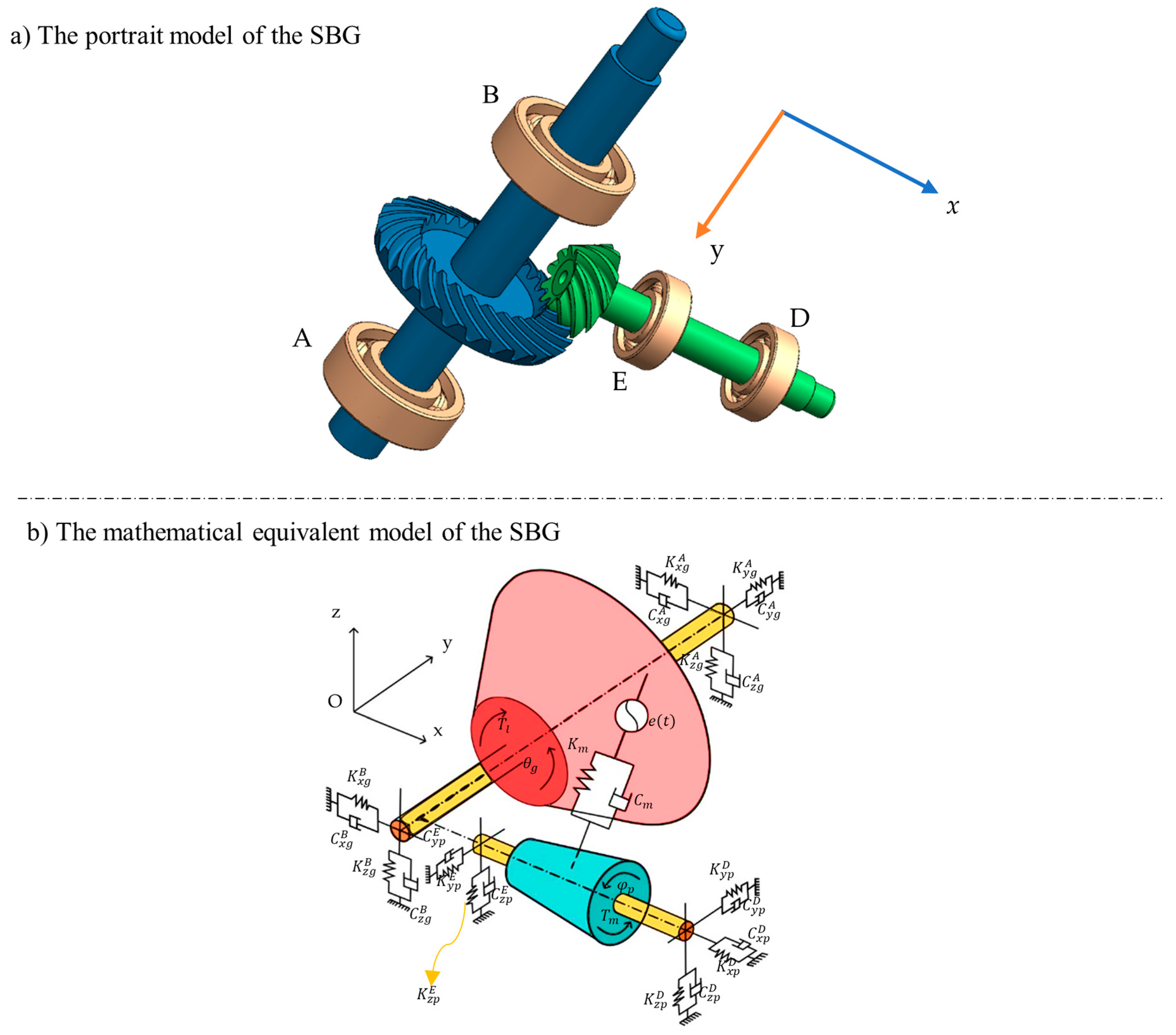
The coordinate system in Figure 1 is selected based on the principal motion directions and symmetry of the gear system. The $x$, $y$, and $z$ axes correspond to lateral, longitudinal, and torsional directions, respectively, which enables the accurate modeling of vibrational behavior. The primary focus of this study is to examine the impact of tolerance stiffness. For this purpose, an eight-degrees of freedom model has been proposed. The mesh stiffness in this model is derived from references, utilizing a transmission error plot.

The governing equations of the dynamic system are provided in Equations (1)–(8). The system’s coordinate vector is expressed as ${[x_p,y_p,z_p,{\phi }_p,x_g,y_g,z_g,{\theta }_g]}^T$ [16].

$$m_p{\ddot{z}}_p+C_{zp}^T{\dot{z}}_p{+K}_{zp}^T{z}_p=-F_n{a}_3$$

(1)

$$m_g{\ddot{z}}_g+C_{zg}^T{\dot{z}}_g+K_{zg}^T{z}_g=F_n{a}_3$$

(2)

$$m_p{\ddot{y}}_p+C_{yp}^T{\dot{y}}_p+K_{yp}^T{y}_p=-F_n{a}_2$$

(3)

$$m_g{\ddot{y}}_g+C_{yg}^T{\dot{y}}_g+K_{yg}^T{y}_g=F_n{a}_2$$

(4)

$$m_p{\ddot{x}}_p+C_{xp}^T{\dot{x}}_p+K_{xp}^T{x}_p=F_n{a}_1$$

(5)

$$m_g{\ddot{x}}_g+C_{xg}^T{\dot{x}}_g+K_{xg}^T{x}_g=-F_n{a}_1$$

(6)

$$I_g^y{\ddot{\theta }}_g=r_g^m\left(F_n\right)a_3-T_l$$

(7)

$$I_p^x{\ddot{\phi }}_p=-r_p^m\left(F_n\right)a_3+T_m$$

(8)

In Equations (1)–(8),

• $K_{zp}^T$ represents the total stiffness of the pinion’s bearings in the $z$-direction;
• $C_{zp}^T$ denotes the damping coefficients of the pinion’s bearings in the $z$-direction, characterized by linear viscous damping;
• Similar definitions apply to other directions.

The parameters $a_1$, $a_2$, $a_3$, $F_n$, $K_{js}^i$, and $C_{js}^i$ in Equations (1)–(8) are defined as follows:

$$a_1=\mathit{sin}\alpha \mathit{sin}\delta +\mathit{sin}\alpha \mathit{sin}\beta \mathit{cos}\delta$$

(9)

$$a_2=\mathit{sin}\alpha \mathit{cos}\delta +\mathit{cos}\alpha \mathit{sin}\beta \mathit{sin}\delta$$

(10)

$$a_3=\mathit{cos}\alpha \mathit{cos}\beta$$

(11)

$$F_n=K_m\left(t\right)f\left(\lambda \right)+C_m\dot{\lambda }$$

(12)

$$\begin{array}{cc}{\overline{K}}_{zp}^T={\displaystyle \frac{K_{zp}^D+K_{zp}^E}{m_p{\omega }_n^2}}& {\overline{C}}_{zp}^T={\displaystyle \frac{C_{zp}^D+C_{zp}^E}{2m_p{\omega }_n}}\\ {\overline{K}}_{zg}^T={\displaystyle \frac{K_{zg}^A+K_{zg}^B}{m_g{\omega }_n^2}}& {\overline{C}}_{zg}^T={\displaystyle \frac{C_{zg}^A+C_{zg}^B}{2m_g{\omega }_n}}\\ {\overline{K}}_{yp}^T={\displaystyle \frac{K_{yp}^D+K_{yp}^E}{m_p{\omega }_n^2}}& {\overline{C}}_{yp}^T={\displaystyle \frac{C_{yp}^D+C_{yp}^E}{2m_p{\omega }_n}}\\ {\overline{K}}_{yg}^T={\displaystyle \frac{K_{yg}^A}{m_g{\omega }_n^2}}& {\overline{C}}_{yg}^T={\displaystyle \frac{C_{yg}^A}{2m_g{\omega }_n}}\\ {\overline{K}}_{xp}^T={\displaystyle \frac{K_{xp}^D}{m_p{\omega }_n^2}}& {\overline{C}}_{xp}^T={\displaystyle \frac{C_{xp}^D}{2m_p{\omega }_n}}\\ {\overline{K}}_{xg}^T={\displaystyle \frac{K_{xg}^A+K_{xg}^B}{m_g{\omega }_n^2}}& {\overline{C}}_{xg}^T={\displaystyle \frac{C_{xg}^A+C_{xg}^B}{2m_g{\omega }_n}}\end{array}$$

(13)

The new dynamic transmission error (DTE) definition for the present eight-degrees of freedom system is defined in Equation (14), while the rotational displacement function, $f\left(\lambda \right)$, is described in Equation (15). In Equation (14), $e\left(t\right)$ denotes the geometric transmission error due to an imperfection in the systems [17], which is mathematically expressed using a Fourier series formulation, as shown in Equation (16).

$$\lambda =\left(-x_p+x_g\right)a_1+\left(y_p-y_g\right)a_2+\left(z_p-z_g+r_p^m{\phi }_p-r_g^m{\theta }_g\right)a_3$$

(14)

$$f(\mathsf{\lambda })=\left\{\begin{array}{ll}\mathsf{\lambda }-\mathrm{e}-\mathrm{b},& \mathsf{\lambda }-\mathrm{e}>b\\ 0,& -b\le \mathsf{\lambda }-\mathrm{e}\le \mathrm{b}\\ \mathsf{\lambda }-\mathrm{e}+\mathrm{b},& \mathsf{\lambda }-\mathrm{e}<-b\end{array}\right.$$

(15)

$$e\left(t\right)=\left\{\begin{array}{ll}{e}^F\left(t\right)=e_0^F+{\displaystyle \sum _{j=1}^s}{ea}_j^F\mathrm{c}\mathrm{o}\mathrm{s}\left(j{\omega }_{m}t\right)+{\displaystyle \sum _{j=1}^s}{ea}_j^F\mathrm{s}\mathrm{i}\mathrm{n}\left(j{\omega }_{m}t\right)& \mathrm{f}\mathrm{o}\mathrm{r}\mathrm{w}\mathrm{a}\mathrm{r}\mathrm{d} \mathrm{m}\mathrm{o}\mathrm{t}\mathrm{i}\mathrm{o}\mathrm{n}\\ e^R\left(t\right)=e_0^R+{\displaystyle \sum _{j=1}^s}{ea}_j^R\mathrm{c}\mathrm{o}\mathrm{s}\left(j{\omega }_{m}t\right)+{\displaystyle \sum _{j=1}^s}{ea}_j^R\mathrm{s}\mathrm{i}\mathrm{n}\left(j{\omega }_{m}t\right)& \mathrm{r}\mathrm{e}\mathrm{v}\mathrm{e}\mathrm{r}\mathrm{s}\mathrm{e} \mathrm{m}\mathrm{o}\mathrm{t}\mathrm{i}\mathrm{o}\mathrm{n}\end{array}\right.$$

(16)

The meshing stiffness of the gear pair varies over time as a periodic function influenced by the excitation mesh frequency ${\omega }_m={\displaystyle \frac{2\pi }{60}}{N}_1{\gamma }_s$. By defining the number of harmonics as $s=\left(N_p-1\right)/2$, Equation (17) provides the Fourier series representation, offering a mathematical expression for the equivalent meshing stiffness. The transmission error is modeled using a truncated Fourier series expansion, where $a_j^R$ and $e_0^R$ denote the amplitude coefficients and the initial phase shift, respectively. These coefficients are used as part of the periodic excitation input in the gear dynamic model [16,18].

$$K_m(t)=k_0+\sum _{j=1}^S{a}_j\mathrm{c}\mathrm{o}\mathrm{s}(j{\omega }_{m}t)+\sum _{j=1}^S{b}_j\mathrm{s}\mathrm{i}\mathrm{n}(j{\omega }_{m}t)$$

(17)

Equations (14), (15) and (17) can be reformulated in terms of the DTE by introducing and substituting new parameters:

$$\begin{array}{c}{\overline{x}}_p={\displaystyle \frac{x_p}{b}}, {\overline{y}}_p={\displaystyle \frac{y_p}{b}}, {\overline{z}}_p={\displaystyle \frac{z_p}{b}}, {\overline{x}}_g={\displaystyle \frac{x_g}{b}}, {\overline{y}}_g={\displaystyle \frac{y_g}{b}}, {\overline{z}}_g={\displaystyle \frac{z_g}{b}}, {\omega }_n=\sqrt{{\displaystyle \frac{K_0}{m_{eq}}}}\\ m_{eq}={\left({\displaystyle \frac{{\left(r_p\right)}^2}{I_p^x}}+{\displaystyle \frac{{\left(r_g\right)}^2}{I_g^y}}\right)}^{-1}\end{array}$$

(18)

$$\overline{\lambda }=\left(-{\overline{x}}_p+{\overline{x}}_g\right)a_1+\left({\overline{y}}_p-{\overline{y}}_g\right)a_2+\left({\overline{z}}_p-{\overline{z}}_g+{\overline{r}}_p{\phi }_p-{\overline{r}}_g{\theta }_g\right)a_3$$

(19)

$$f(\overline{\lambda })=\left\{\begin{array}{ll}\overline{\lambda }-\overline{e}-1,& \overline{\lambda }-\overline{e}>1\\ 0,& -1\le \overline{\lambda }-\overline{e}\le 1\\ \overline{\lambda }-\overline{e}+1,& \overline{\lambda }-\overline{e}<-1\end{array}\right.$$

(20)

$$\overline{K}\left(t\right)=1+\sum _{j=1}^7{\displaystyle \frac{a_j}{m_{eq}{\omega }_n^2}}\mathrm{c}\mathrm{o}\mathrm{s}(j{\omega }_{m}t)+\sum _{j=1}^7{\displaystyle \frac{b_j}{m_{eq}{\omega }_n^2}}\mathrm{s}\mathrm{i}\mathrm{n}(j{\omega }_{m}t)$$

(21)

To normalize the governing equation, the following new parameters are introduced:

$$\begin{array}{rrrrr}\xi ={\displaystyle \frac{C_m}{2m_{eq}{\omega }_n}},& {\overline{T}}_m={\displaystyle \frac{1}{b{m}_{eq}{\omega }_n^2}}\left({\displaystyle \frac{T_m}{r_p}}\right),& \tau ={\omega }_{n}t,& \ddot{\lambda }={\omega }_n^2{\lambda }^{″},& \dot{\lambda }={\omega }_n{\lambda }^{\prime }\\ {\overline{K}}_p\left(t\right)={\displaystyle \frac{K_m\left(t\right)}{m_p{\omega }_n^2}},& {\overline{C}}_p={\displaystyle \frac{C_m}{2m_p{\omega }_n}},& \ddot{z}={\omega }_n^2{z}^{″},& \ddot{y}={\omega }_n^2{y}^{″},& \ddot{x}={\omega }_n^2{x}^{″}\\ {\overline{K}}_g\left(t\right)={\displaystyle \frac{K_m\left(t\right)}{m_g{\omega }_n^2}},& {\overline{C}}_g={\displaystyle \frac{C_m}{2m_g{\omega }_n}},& \dot{z}={\omega }_n{z}^{\prime },& \dot{y}={\omega }_n{y}^{\prime },& \dot{x}={\omega }_n{x}^{\prime }\\ & & {\lambda }^{\prime }={\displaystyle \frac{\mathrm{d}\lambda }{\mathrm{d}\tau }}& \dot{\lambda }={\displaystyle \frac{\mathrm{d}\lambda }{\mathrm{d}t}}& \end{array}$$

(22)

Accordingly, Equations (1)–(8) can be rewritten in the following alternative forms:

$${\overline{\lambda }}^{″}+a_3^2\overline{K}\left(t\right)f\left(\overline{\lambda }\right)+2a_3^2\xi {\overline{\lambda }}^{\prime }-\left(\left(-{\overline{x}}_p^{″}+{\overline{x}}_g^{″}\right)a_1+\left({\overline{y}}_p^{″}-{\overline{y}}_g^{″}\right)a_2+\left({\overline{z}}_p^{″}-{\overline{z}}_g^{″}\right)a_3\right)={\overline{T}}_m{a}_3$$

(23)

$${\overline{z}}_p^{″}+{\overline{K}}_{zp}^T{\overline{z}}_p+2{\overline{C}}_{zp}^T{\overline{z}}_p^{\prime }=-{\overline{K}}_p\left(t\right)f\left(\overline{\lambda }\right)a_3-2{\overline{C}}_p{\overline{\lambda }}^{\prime }{a}_3$$

(24)

$${\overline{z}}_g^{″}+{\overline{K}}_{zg}^T{\overline{z}}_g+2{\overline{C}}_{zg}^T{\overline{z}}_g^{\prime }=+{\overline{K}}_g\left(t\right)f\left(\overline{\lambda }\right)a_3+{\overline{C}}_g{\overline{\lambda }}^{\prime }{a}_3$$

(25)

$${\overline{y}}_p^{″}+{\overline{K}}_{yp}^T{\overline{y}}_p+2{\overline{C}}_{yp}^T{\overline{y}}_p^{\prime }=-{\overline{K}}_p\left(t\right)f\left(\overline{\lambda }\right)a_2-2{\overline{C}}_p{\overline{\lambda }}^{\prime }{a}_2$$

(26)

$${\overline{y}}_g^{″}+{\overline{K}}_{yg}^T{\overline{y}}_g+2{\overline{C}}_{yg}^T{\overline{y}}_g^{\prime }={\overline{K}}_g\left(t\right)f\left(\overline{\lambda }\right)a_2+2{\overline{C}}_g{\overline{\lambda }}^{\prime }{a}_2$$

(27)

$${\overline{x}}_p^{″}+{\overline{K}}_{xp}^T{\overline{x}}_p+2{\overline{C}}_{xp}^T{\overline{x}}_p^{\prime }={\overline{K}}_p\left(t\right)f\left(\overline{\lambda }\right)a_1+2{\overline{C}}_p{\overline{\lambda }}^{\prime }{a}_1$$

(28)

$${\overline{x}}_g^{″}+{\overline{K}}_{xg}^T{\overline{x}}_g+2{\overline{C}}_{xg}^T{\overline{x}}_g^{\prime }=-{\overline{K}}_g\left(t\right)f\left(\overline{\lambda }\right)a_1-2{\overline{C}}_g{\overline{\lambda }}^{\prime }{a}_1$$

(29)

3. Validation

To validate the simulated numerical results, amplitude–frequency diagrams based on the root mean square (RMS) of the dynamic transmission error are compared in Figure 2 with the results of Ref. [19]. Figure 2a represents only one case from Ref. [19], and Figure 2b presents the RMS of this study considering high lateral bearing stiffness. The validation is performed using the blue curve shown in Figure 2a. The close agreement between these two graphs confirms the accuracy of the model and the correctness of the present results. A comparison of RMS variations across different frequency ranges further demonstrates that the simulated dynamic behavior aligns well with the reference data, reinforcing the reliability of the simulation. In all four cases, the bearing stiffness was considered constant.

The comparison between the simulation results and the reference data confirms the validity of the proposed dynamic model. The root mean square (RMS) of the dynamic transmission error (DTE), as depicted in Figure 2, aligns closely with the established benchmark, particularly under high lateral bearing stiffness. This agreement demonstrates that the model accurately captures key vibrational characteristics of spiral bevel gears.

4. Considered SBG Cases to Apply Modifications

This paper investigated four cases, each of which is described individually in this section. Along with converting the transmission error graph to the mesh stiffness, the corresponding mesh stiffness graph for each case is also presented in this section. Following the conversion, the results are analyzed, and the vibrational behavior of each case is studied. The cases examined in this study are presented in

Table 1. Reviewed cases and their modification methods.

Cases Reviewed	Year of Research	Method
Case 1, [1]	2010	Topology modification
Case 2, [2]	2014	Topology modification
Case 3, [3]	2018	Flank modification
Case 4, [4]	2020	Flank modification

, along with the method of tooth profile modification.

Topological modification involves complex, three-dimensional adjustments to the entire tooth surface, allowing asymmetric or curved contact paths to optimize load distribution and dynamic performance. In contrast, flank modification refers to conventional, often symmetric corrections, such as profile or lead crowning, tip relief, and end relief, aimed at compensating for misalignment, deflections, and manufacturing errors. While flank modifications are typically standardized and localized, topological modifications offer greater design flexibility for advanced performance requirements.

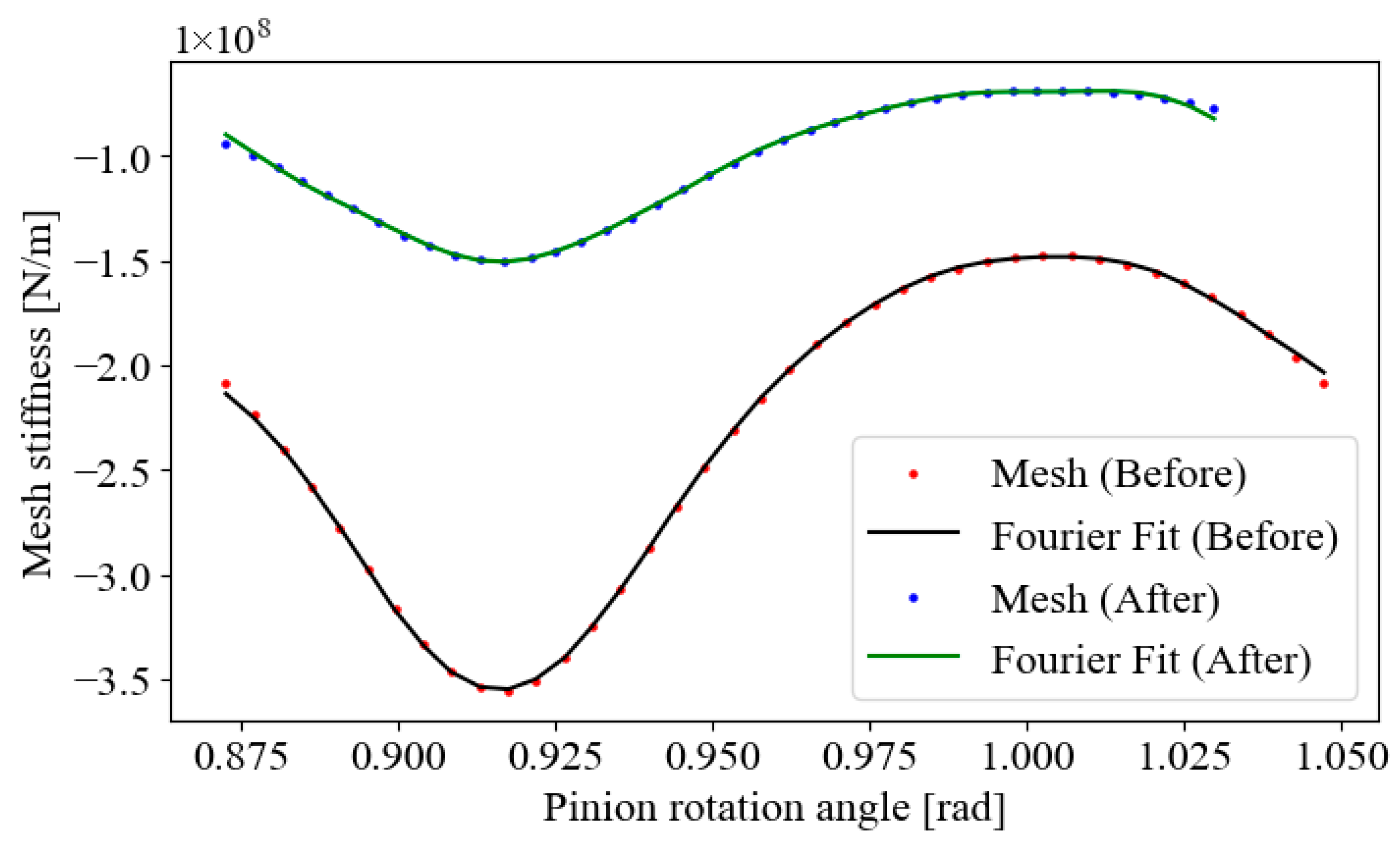
The gear pair properties for the first case are summarized in

Table 2. Gear pair properties for Case 1.

Title	Pinion	Gear
Number of teeth	14	41
Module	3.105
Base circle radius (mm)	20.3	119.62
Pressure angle (deg)	20
Backlash (mm)	0.150
Torque (N·m)	250

[1], and the mesh stiffness diagram is depicted in Figure 3 by expressing a fifth-order Fourier series expansion. The mesh stiffness diagram for Case 1 is presented before and after the modifications in the following figure.

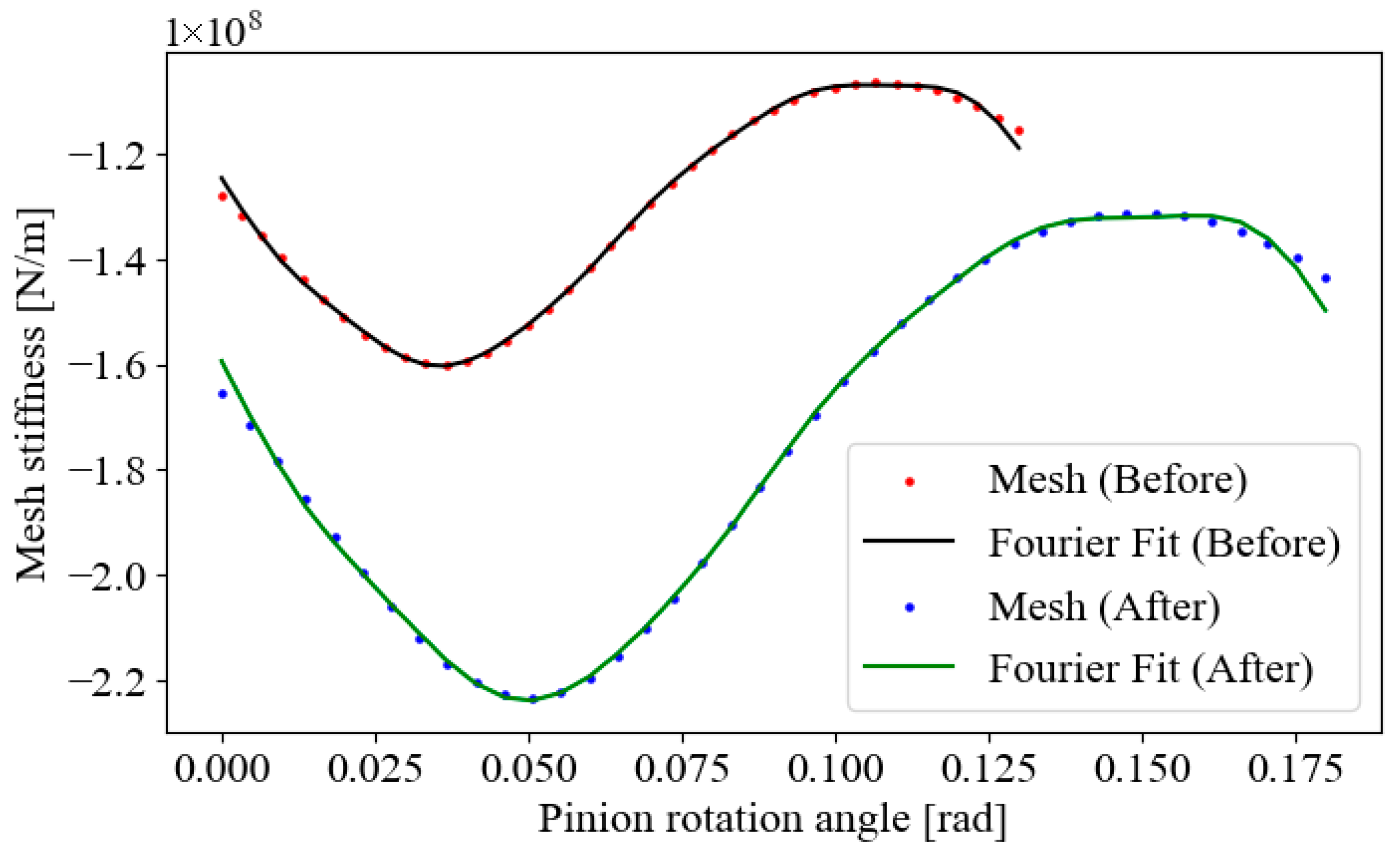
The gear pair properties and mesh stiffness diagram for Case 2 [2] are presented in

Table 3. Gear pair properties for Case 2.

Title	Pinion	Gear
Number of teeth	15	44
Module	5.8
Base circle radius (mm)	43.5	119.90
Pressure angle (deg)	20
Backlash (mm)	0.3
Torque (N·m)	260

and Figure 4.

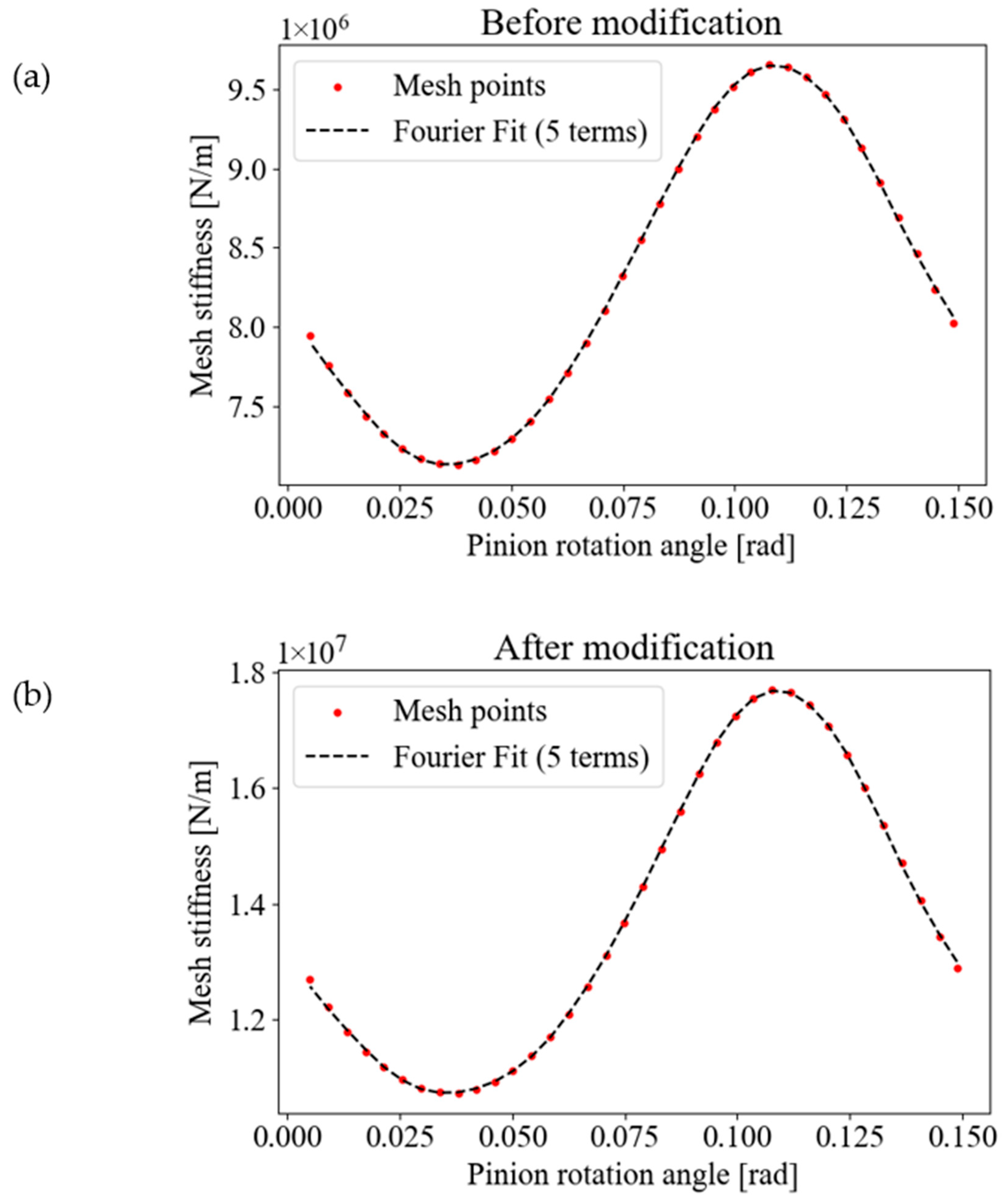
Gear pair properties and mesh stiffness diagram for Case 3 [3] are presented in

Table 4. Gear pair properties for Case 3.

Title	Pinion	Gear
Number of teeth	23	65
Module	3.9
Base circle radius (mm)	42.14	119.10
Pressure angle (deg)	20
Backlash (mm)	0.7
Torque (N·m)	1000

and Figure 5.

Gear pair properties and mesh stiffness diagram for Case 4 [4] are presented in

Table 5. Gear pair properties for Case 4.

Title	Pinion	Gear
Number of teeth	23	65
Module	7
Base circle radius (mm)	75.65	213.78
Pressure angle (deg)	20
Backlash (mm)	0.7
Torque (N·m)	20,000

and Figure 6.

Numerical Results and Discussion

This section addresses the vibrational behavior of the systems, where the responses are obtained by solving the non-smooth second-order ordinary differential equations using the Runge–Kutta method. Subsequently, the responses are extracted through numerical solutions. To capture all possible system’s responses, forward and backward simulations are conducted. Different dynamical tools are employed to evaluate the dynamics of the systems, such as amplitude–frequency diagram, bifurcation analysis, phase portraits, and Poincaré maps. The analysis method began with an examination of the amplitude–frequency diagram, followed by an analysis of the vibration levels of the system. The natural frequency in the investigated system is considered equivalent to that of a single-degree of freedom system representing the studied model. In this study, chaotic motion is identified qualitatively through scattered Poincaré maps and irregular phase portraits, indicating sensitivity to initial conditions and the absence of periodicity. The parameters used in the simulations were chosen based on previous validated models in the literature [16], with minor adjustments to match the system under study.

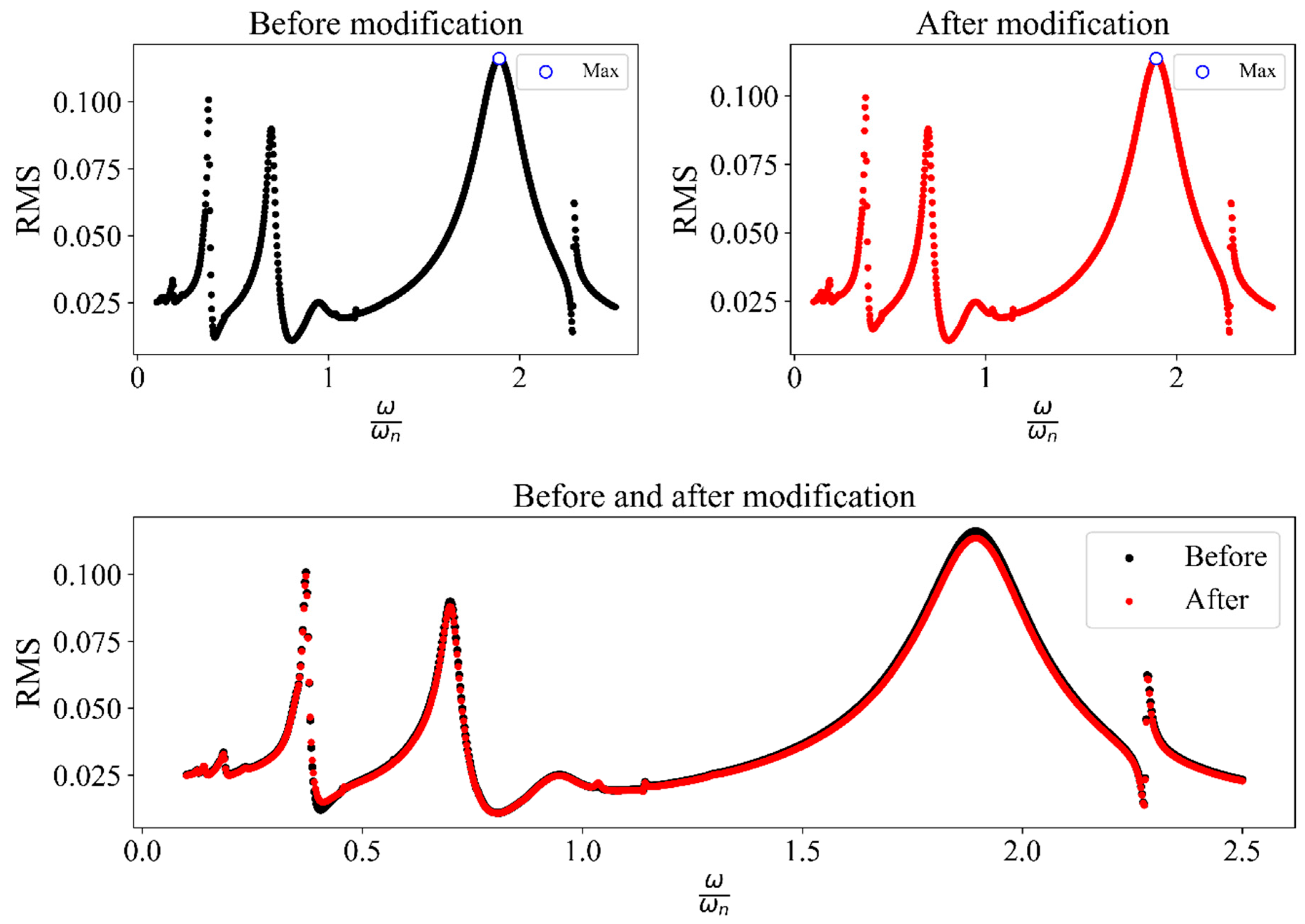
As shown in Figure 7, the highest vibration level of the system occurs at ${\displaystyle \raisebox{1ex}{$\omega $}\!\left/ \!\raisebox{-1ex}{${\omega }_n$}\right.}\approx 1.5$, where before the modifications, this value was 0.10, and after the modifications, it decreased to 0.08. Additionally, in the comparative diagram, it is evident that the vibration level has decreased.

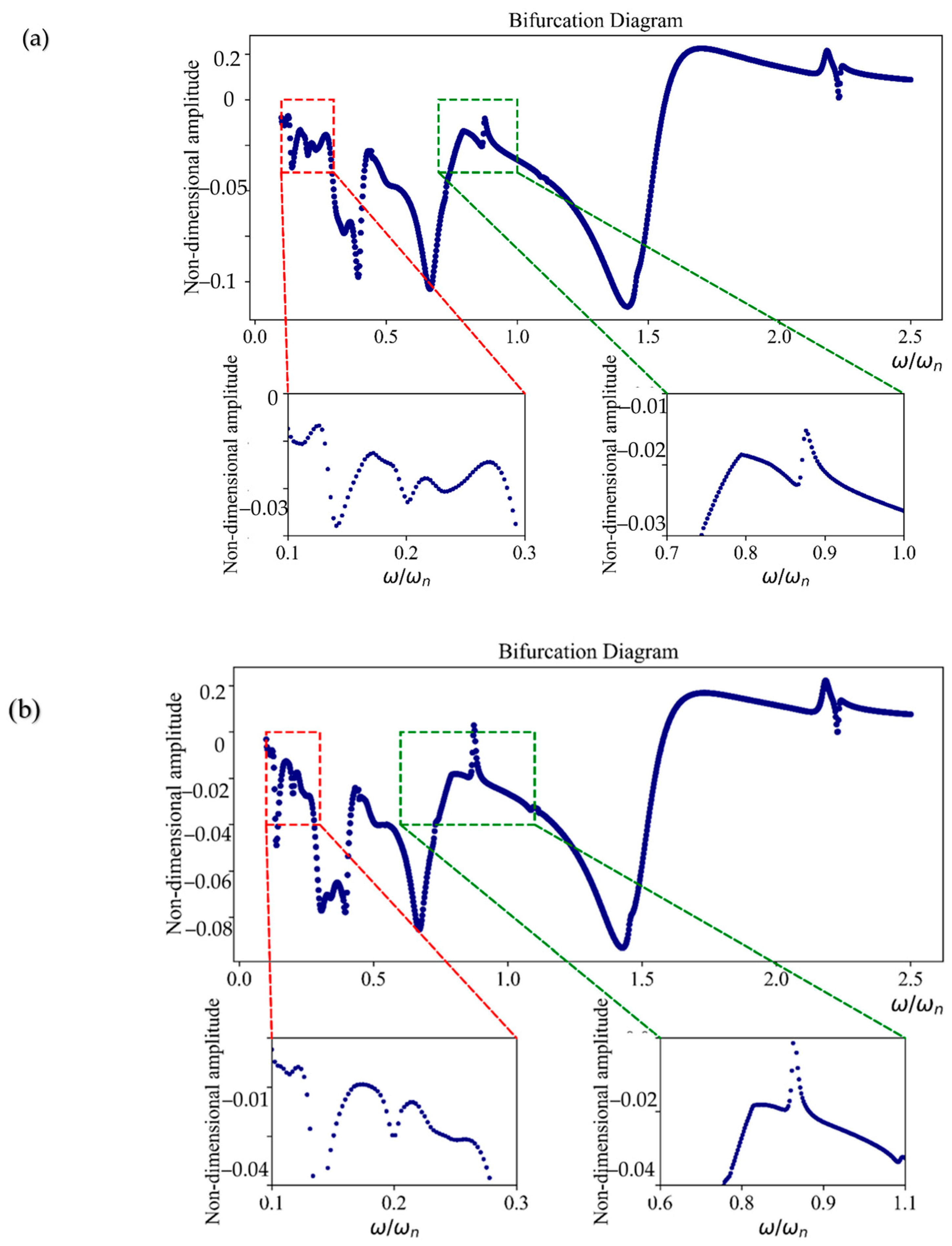
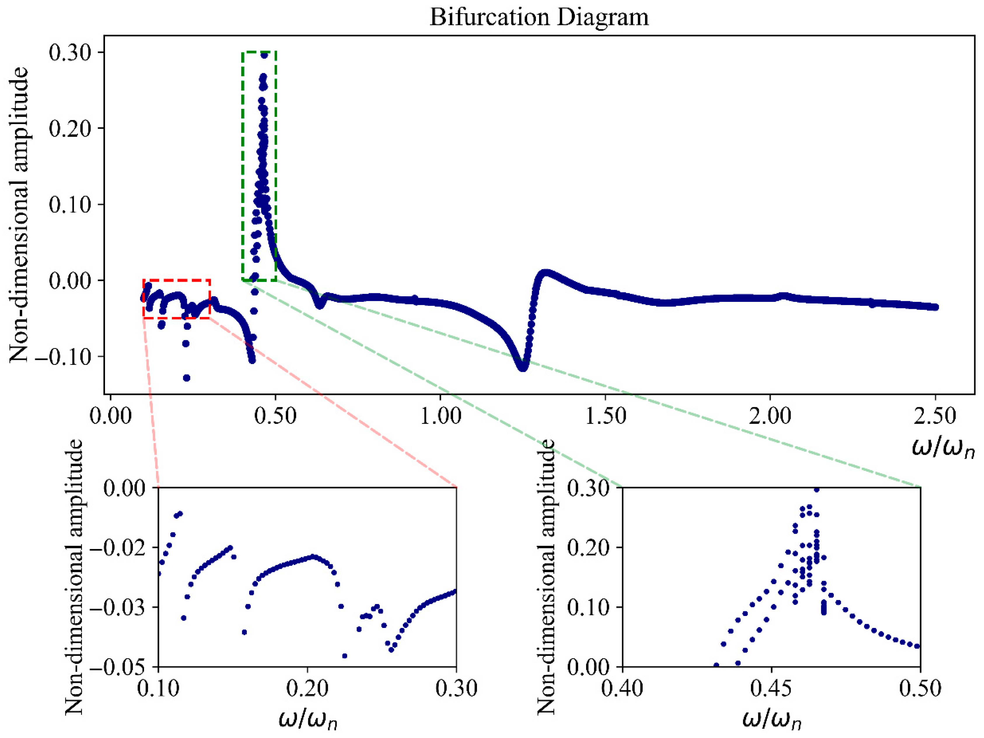
Figure 8 shows the bifurcation diagram of Case 1 before and after the modifications. Upon further analysis, two suspicious regions are identified, which are highlighted below the diagrams. In these regions, it is observed that the vibrational behavior of the system, both before and after the modifications, remains completely periodic, with no occurrence of phenomena such as chaos. For the analysis of Case 2, similar to Case 1, the amplitude–frequency diagram is first examined, as shown in Figure 8.

As shown in Figure 9, a peak is observed at a frequency of ${\displaystyle \raisebox{1ex}{$\omega $}\!\left/ \!\raisebox{-1ex}{${\omega }_n$}\right.}\approx 1.9$ both before and after the modifications, with a reduction in vibration amplitude of approximately 0.01. However, in the bifurcation diagram of Case 2, four suspicious regions are identified. Upon closer examination of these regions, it is evident that the vibrational behavior of this case also remains completely periodic. Refer to Figure 9 and Figure 10 for details.

For the analysis of Case 3, similar to the previous two cases, the RMS diagram is examined first. Refer to Figure 11, where the diagrams indicate a significant reduction in vibration levels for Case 2 after the modifications. In this case, the maximum vibration level occurs at a frequency of ${\displaystyle \raisebox{1ex}{$\omega $}\!\left/ \!\raisebox{-1ex}{${\omega }_n$}\right.}\approx 1.4$.

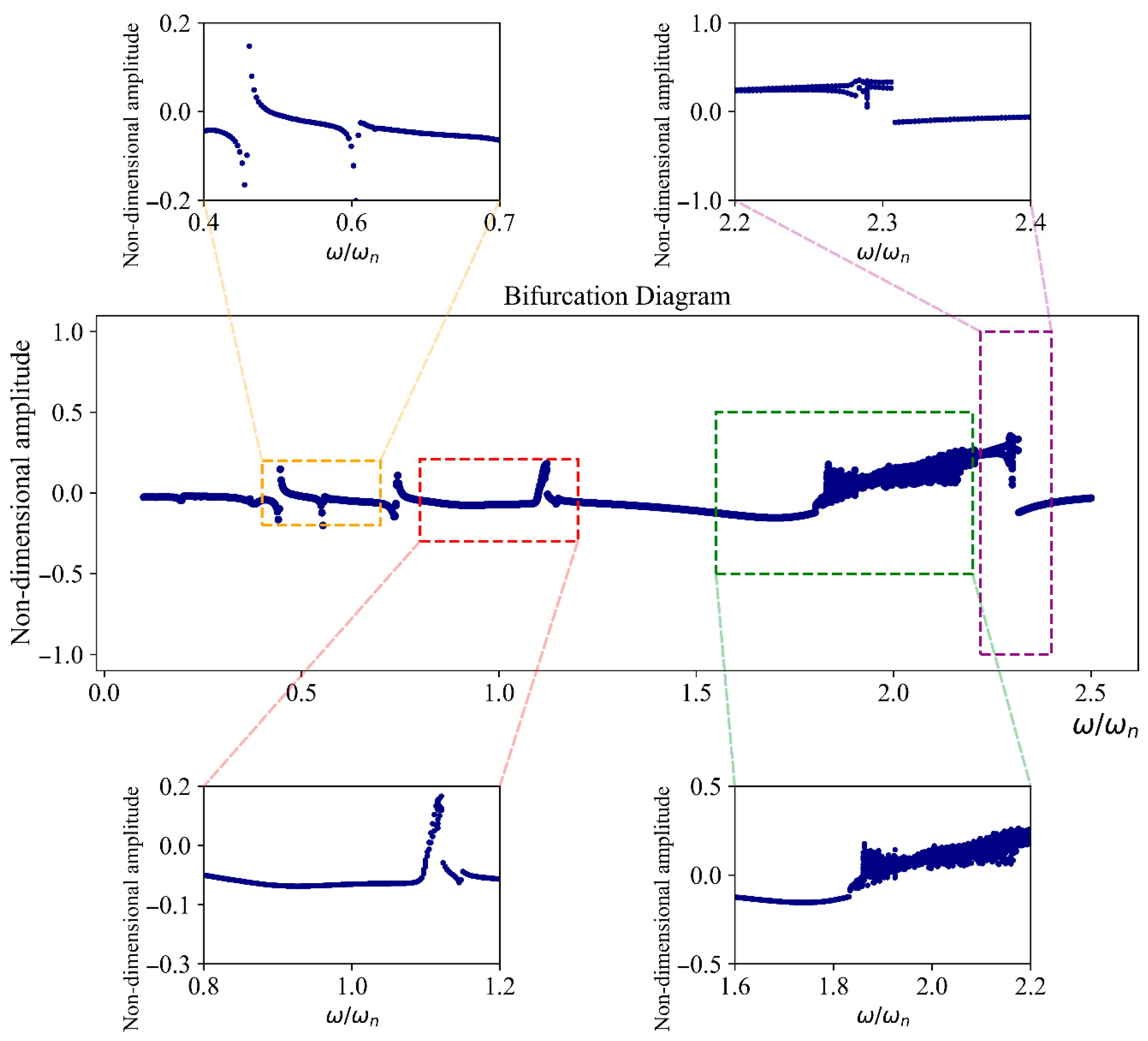
To analyze the vibrational behavior of the system before and after the modifications, it is necessary to examine the bifurcation diagram. Figure 12 illustrates the diagram for the system before the modifications.

Refer to Figure 13, which highlights regions of suspicious vibrational behavior, as shown in four specific areas. By analyzing these regions within a narrow frequency range and with greater detail, it becomes evident that further examination of the system’s vibrational behavior requires studying the phase portraits and Poincaré maps. As depicted in this figure, such diagrams are provided for the four regions at specific frequencies: region 1 at ${\displaystyle \raisebox{1ex}{$\omega $}\!\left/ \!\raisebox{-1ex}{${\omega }_n$}\right.}\approx 0.6$; region 2 at ${\displaystyle \raisebox{1ex}{$\omega $}\!\left/ \!\raisebox{-1ex}{${\omega }_n$}\right.}\approx 1.11$; region 3 at ${\displaystyle \raisebox{1ex}{$\omega $}\!\left/ \!\raisebox{-1ex}{${\omega }_n$}\right.}\approx 1.7$; and region 4 at ${\displaystyle \raisebox{1ex}{$\omega $}\!\left/ \!\raisebox{-1ex}{${\omega }_n$}\right.}\approx 2.30$.

From the analysis, the following is clear:

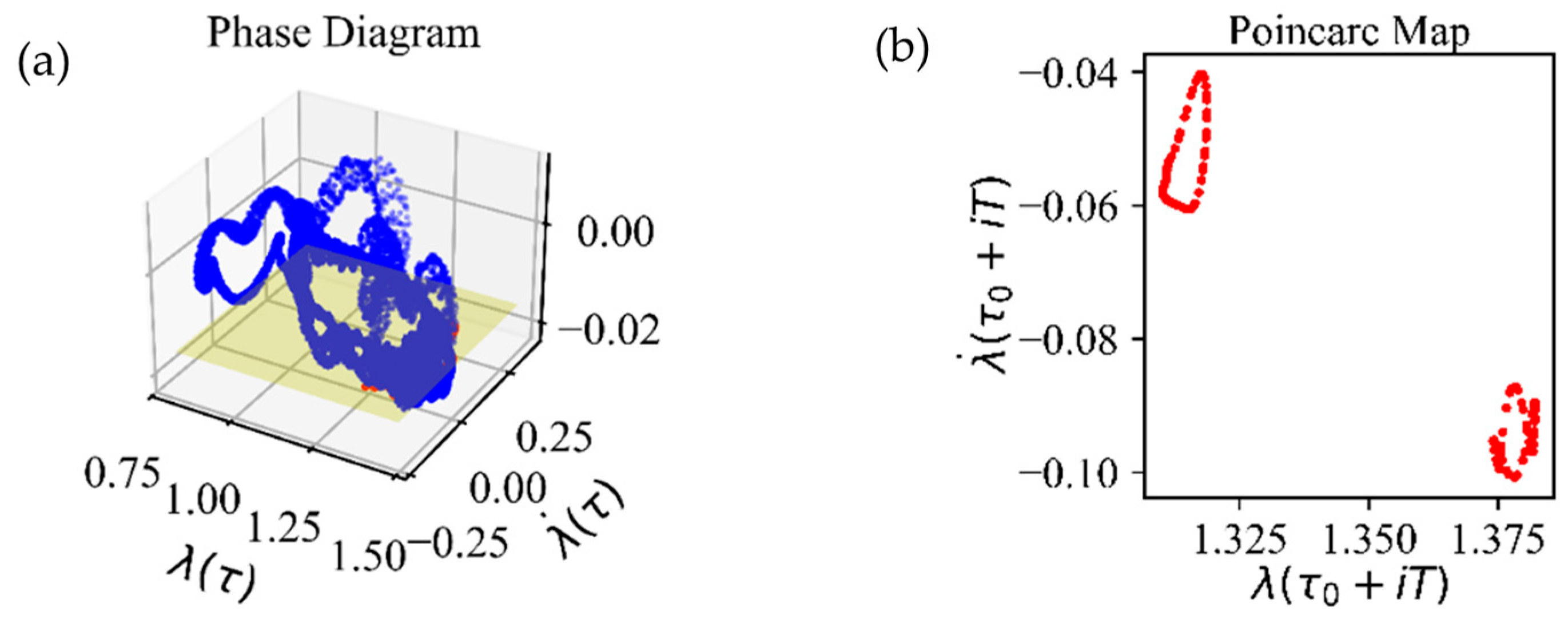
• In region 1, the system exhibits completely periodic behavior, indicating no risk to its stability. It should be noted that in the phase diagram there is only one closed curve, which may appear as three separate closed curves due to its complex shape.
• However, in regions 2, 3, and 4, the system demonstrates chaotic behavior, posing potential risks to its performance.

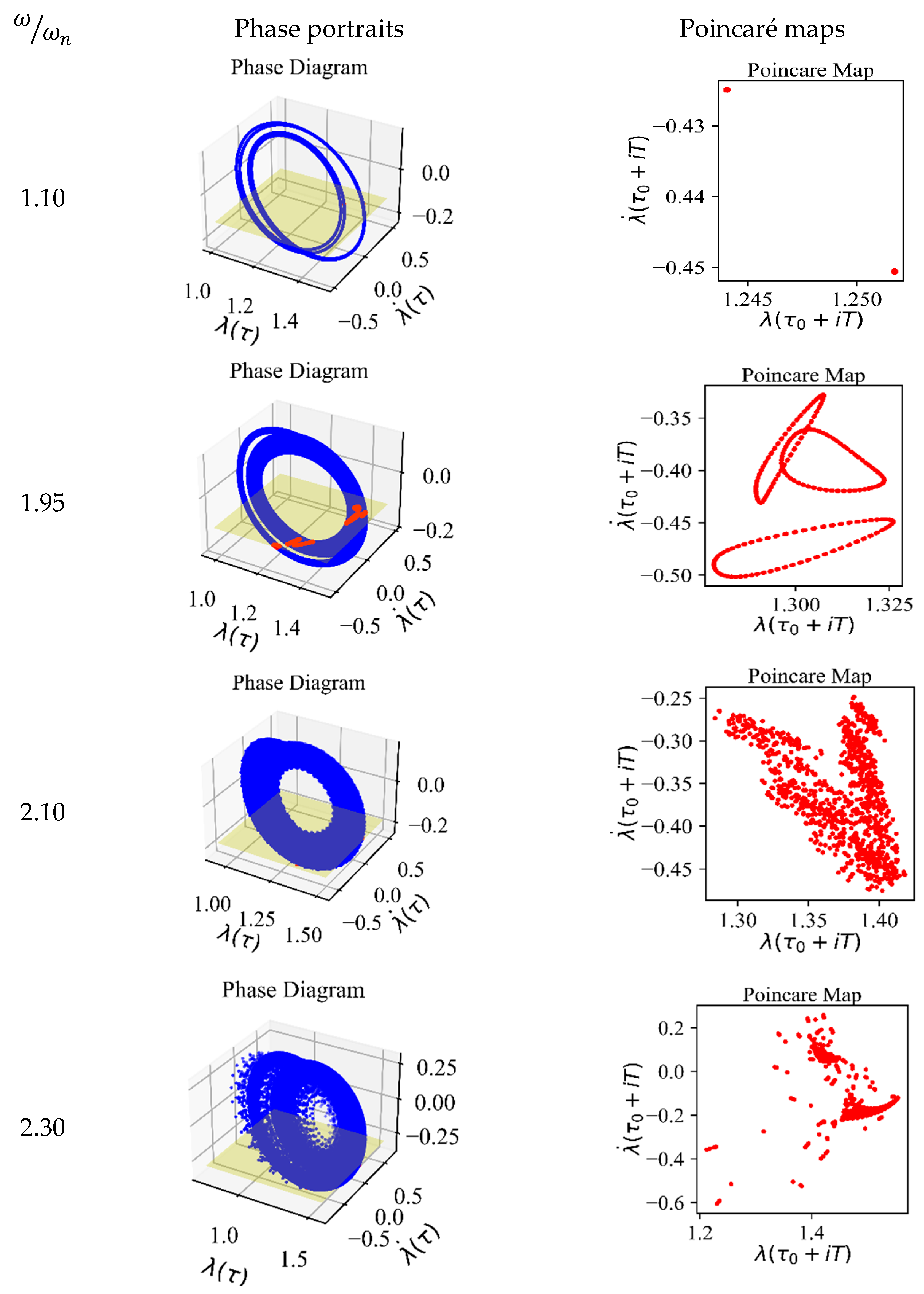
Figure 14 illustrates that the system’s vibrational behavior remains suspicious in the same regions identified earlier. In region 1, the behavior is still periodic, indicating stability. However, for the remaining three regions, a detailed analysis of phase portraits and Poincaré maps is necessary to accurately assess the system’s vibrational behavior and gain further insights.

As shown in Figure 15, within the frequency range of 1 to 1.1, the system’s behavior transitions from chaos to a two-periodic response, indicating an improvement in the vibrational behavior in this range. However, in the other regions, no significant changes are observed, and the system’s vibrational response remains chaotic, posing a potential risk to its stability. A nonlinear time series analysis is conducted to estimate the Largest Lyapunov Exponent (LLE) for Case 3 at different excitation frequencies, where a positive value indicates an irregular response and a negative value corresponds to periodic behavior (see

Table 6. Largest Lyapunov exponent estimation for different excitation frequencies of Case 3.

$\raisebox{1ex}{$\mathit{\omega }$}\!\left/ \!\raisebox{-1ex}{${\mathit{\omega }}_{\mathit{n}}$}\right.$—After	1.10—After	1.95—After	2.10—After	2.30—After
LLE	−0.0015	+0.046	+0.085	+0.009
$\raisebox{1ex}{$\mathit{\omega }$}\!\left/ \!\raisebox{-1ex}{${\mathit{\omega }}_{\mathit{n}}$}\right.$—Before	0.6—Before	Case 2—Before	Case 3—Before	Case 4—Before
LLE	−0.0045	+0.087	+0.068	+0.047

).

Figure 16 shows the RMS diagrams for Case 4, indicating a reduction in the system’s vibration levels. This demonstrates an improvement in the vibrational performance of this case as well.

To analyze the vibrational behavior of this case, Figure 17 present the bifurcation diagram before the modifications.

Based on the bifurcation diagram, the system’s vibrational behavior exhibits two suspicious regions. In the range of 0.3 to 0.4, the system demonstrates periodic behavior, while in the range of 0.4 to 0.5, the behavior is uncertain and requires further analysis through Poincaré maps and phase portraits, as shown in Figure 18. It is evident that at a ${\displaystyle \raisebox{1ex}{$\omega $}\!\left/ \!\raisebox{-1ex}{${\omega }_n$}\right.}\approx 0.45$, the system undergoes chaotic behavior.

To analyze the vibrational behavior of the system after the modifications, refer to Figure 19. This figure illustrates the system’s bifurcation diagram, which, similarly to the previous diagram, contains two suspicious regions. The first region, as before, exhibits periodic behavior, while the second region requires further examination through phase portraits and Poincaré maps.

Refer to Figure 20, where it is evident that the system’s vibrational behavior has improved, transitioning from chaotic behavior to a 10-periodic response at a ${\displaystyle \raisebox{1ex}{$\omega $}\!\left/ \!\raisebox{-1ex}{${\omega }_n$}\right.}\approx 0.45$.

5. Discussion

The present study examined the nonlinear dynamic response of spiral bevel gear systems under four different profile modification scenarios. Through detailed bifurcation analysis, Poincaré maps, and RMS comparisons, it was observed that certain modifications—particularly flank corrections—led to both a reduction in vibration amplitude and the suppression of chaotic behavior.

Table 7. Quantitative comparison of vibration amplitudes before and after applying profile modifications for all four cases.

Case	Max Amplitude (Before)	Max Amplitude (After)	Reduction (%)
1	0.1	0.08	20
2	0.12	0.11	8.33
3	0.68	0.21	69.12
4	0.34	0.28	17.65

summarizes the percentage change in peak vibration amplitude before and after applying the profile modifications for each case.

In Cases 1 and 2, which involved topological modifications, a moderate decrease in vibration levels was detected (20% and 8.3%, respectively), yet the system dynamics remained largely periodic before and after the changes. This indicates that while topological modifications enhance amplitude response by improving load distribution, they might not be sufficient for altering the qualitative nature of system dynamics under all conditions.

Conversely, Cases 3 and 4, which implemented flank modifications, demonstrated more substantial improvements. In Case 3, the maximum amplitude dropped by approximately 69%, and chaotic motion observed in three distinct frequency regions was effectively suppressed in at least one of them. Similarly, in Case 4, the system exhibited a transition from chaos to a 10-periodic response, showing improved stability.

These outcomes underscore the fact that flank modifications not only reduce vibrational amplitude but also influence the system’s stability landscape, pushing chaotic regimes toward more ordered behaviors. The findings align with previous studies that highlight the sensitivity of gear dynamics to local geometry corrections, particularly at the meshing interface.

From a practical perspective, all proposed modifications are achievable using modern manufacturing technologies, such as five-axis CNC milling and precision grinding. However, real-world implementation requires the careful assessment of manufacturing costs, long-term durability under cyclic loading, and integration into current gear design standards.

6. Conclusions

From a practical standpoint, the proposed profile and flank modifications are feasible using modern manufacturing techniques such as CNC grinding, five-axis machining, and precision forging. These methods allow for controlled geometry adjustments with high repeatability. In high-performance applications such as automotive or aerospace gearboxes, even minor improvements in vibrational behavior can lead to significantly enhanced durability and noise reduction. However, further work is needed to assess cost implications, fatigue behavior under load cycles, and integration into existing gear design workflows. This study investigates a SBG system with eight degrees of freedom, incorporating modifications into the tooth profile. Different vibrational responses were observed for each type of modification, and each modification was analyzed separately. The responses varied depending on the type of modification applied. The results of this study demonstrated that the vibration levels of the system decrease with the modifications, indicating an improvement in the system’s vibrational behavior, which positively impacts the system’s lifespan. Additionally, in some cases, improvements in the vibrational behavior of the system were observed, which can also have a positive effect on the system’s longevity. A more detailed analysis revealed that modifications to the tooth profile had a noticeable impact on the system’s vibration levels, although they did not lead to significant changes in the vibrational behavior. However, modifications to the topology not only reduced the vibration levels but also contributed to an improvement in the system’s vibrational behavior.

If we classify the conclusions based on the type of modification, they can be divided into two main categories:

• Tooth Topology Modifications: This type of modification had a 20% significant impact on vibration levels, as seen in Case 1, and an 8% impact in Case 2. As observed, these modifications reduced the vibration levels in these two cases but did not significantly affect the vibrational behavior of the system.
• Tooth Flank Modifications: In this type of modification, a 69% reduction in the vibration levels was observed in Case 3, along with a 17% reduction in Case 4. This modification not only reduced the vibration levels but also improved the vibrational behavior of the system.

References

- Shih, Y.-P. A novel ease-off flank modification methodology for spiral bevel and hypoid gears. Mech. Mach. Theory 2010, 45, 1108–1124. [Google Scholar] [CrossRef]
- Astoul, J.; Mermoz, E.; Sartor, M.; Linares, J.M.; Bernard, A. New methodology to reduce the transmission error of the spiral bevel gears. CIRP Ann. 2014, 63, 165–168. [Google Scholar] [CrossRef]
- Mu, Y.; Li, W.; Fang, Z.; Zhang, X. A novel tooth surface modification method for spiral bevel gears with higher-order transmission error. Mech. Mach. Theory 2018, 126, 49–60. [Google Scholar] [CrossRef]
- Mu, Y.; Li, W.; Fang, Z. Tooth surface modification method of face-milling spiral bevel gears with high contact ratio based on cutter blade profile correction. Int. J. Adv. Manuf. Technol. 2020, 106, 3229–3237. [Google Scholar] [CrossRef]
- Korka, Z. An overview of mathematical models used in gear dynamics. Rom. J. Acoust. Vib. 2007, 4, 43–50. [Google Scholar]
- Molaie, M.; Zippo, A.; Pellicano, F. Chaotic dynamics of spiral bevel gears. Int. J. Non-Linear Mech. 2025, 175, 105098. [Google Scholar] [CrossRef]
- Samani, F.S.; Salajegheh, M.; Molaie, M. Nonlinear vibration of the spiral bevel gear under periodic torque considering multiple elastic deformation evaluations due to different bearing supports. SN Appl. Sci. 2021, 3, 772. [Google Scholar] [CrossRef]
- Motahar, H.; Samani, F.S.; Molaie, M. Nonlinear vibration of the bevel gear with teeth profile modification. Nonlinear Dyn. 2016, 83, 1875–1884. [Google Scholar] [CrossRef]
- Li, H.; Tang, J.; Chen, S.; Rong, K.; Ding, H.; Lu, R. Loaded contact pressure distribution prediction for spiral bevel gear. Int. J. Mech. Sci. 2023, 242, 108027. [Google Scholar] [CrossRef]
- Molaie, M.; Samani, F.S.; Motahar, H. Nonlinear vibration of crowned gear pairs considering the effect of Hertzian contact stiffness. SN Appl. Sci. 2019, 1, 414. [Google Scholar] [CrossRef]
- Su, X.; Tomovic, M.M.; Zhu, D. Diagnosis of gradual faults in high-speed gear pairs using machine learning. J. Braz. Soc. Mech. Sci. Eng. 2019, 41, 195. [Google Scholar] [CrossRef]
- Xu, J.; Wan, L.; Luo, W. Influence of bearing stiffness on the nonlinear dynamics of a shaft-final drive system. Shock. Vib. 2016, 2016, 1–14. [Google Scholar] [CrossRef]
- Yang, J.J.; Shi, Z.H.; Zhang, H.; Li, T.X.; Nie, S.W.; Wei, B.Y. Dynamic analysis of spiral bevel and hypoid gears with high-order transmission errors. J. Sound Vib. 2018, 417, 149–164. [Google Scholar] [CrossRef]
- Samani, F.S.; Molaie, M.; Pellicano, F. Nonlinear vibration of the spiral bevel gear with a novel tooth surface modification method. Meccanica 2019, 54, 1071–1081. [Google Scholar] [CrossRef]
- Wang, H.; Yan, C.; Zhou, C.; Hu, B.; Dong, J.; Yin, L. A loaded tooth contact analysis (LTCA) model of profile-modified gears. Meccanica 2024, 60, 17–37. [Google Scholar] [CrossRef]
- Samani, F.S.; Molaie, M.; Rakhshani, S.; Asadi, M.; Zippo, A.; Iarriccio, G. Nonlinear dynamics of spiral bevel gear: Axial bearing stiffness effect. In Advances in Italian Mechanism Science; Springer Nature: Cham, Switzerland, 2024. [Google Scholar] [CrossRef]
- Molaie, M.; Deylaghian, S.; Iarriccio, G.; Samani, F.S.; Zippo, A.; Pellicano, F. Planet load-sharing and phasing. Machines 2022, 10, 634. [Google Scholar] [CrossRef]
- Molaie, M.; Samani, F.S.; Zippo, A.; Iarriccio, G.; Pellicano, F. Spiral bevel gears: Bifurcation and chaos analyses of pure torsional system. Chaos Solitons Fractals 2023, 177, 114179. [Google Scholar] [CrossRef]
- Molaie, M.; Samani, F.S.; Zippo, A.; Pellicano, F. Spiral bevel gears: Nonlinear dynamic model based on accurate static stiffness evaluation. J. Sound Vib. 2023, 544, 117434. [Google Scholar] [CrossRef]
Figure 1.
Dynamical model of considered SBG with lateral DOF.
Figure 2.
RMS comparison. (
a): RMS graph from Ref. [
19], (
b): RMS graph of the present study considering huge lateral bearing stiffness.
Figure 3.
Mesh stiffness diagram for Case 1 (before and after modifications).
Figure 4.
Mesh stiffness diagram: Case 2 (before and after modifications).
Figure 5.
Mesh stiffness diagram for Case 3 (a) before modification and (b) after modification.
Figure 6.
Mesh stiffness diagram for Case 4 (a) before modification and (b) after modification.
Figure 7.
RMS plots for Case 1 (before and after modification).
Figure 8.
Bifurcation diagram for Case 1 ((a): before modification; (b): after modification).
Figure 9.
RMS plots for Case 2 (before and after modification).
Figure 10.
Bifurcation diagram for Case 2 before modification.
Figure 11.
Bifurcation diagram Case 2 after modification.
Figure 12.
RMS plots for Case 3 (before and after modification).
Figure 13.
Bifurcation diagram, Poincaré maps, and phase portraits for Case 3 before modifications. Region 1 shows the periodic behavior; regions 2–4 exhibit chaotic motion.
Figure 14.
Bifurcation diagram for Case 3 (after modifications).
Figure 15.
Poincaré maps and phase portraits for Case 3 (after modifications).
Figure 16.
RMS plots for Case 4 (before and after modification).
Figure 17.
Bifurcation diagram for Case 4 before modifications.
Figure 18.
Poincaré Map and phase portrait for Case 4 (before modifications).
Figure 19.
Bifurcation diagram for Case 4 (after modifications).
Figure 20.
Poincaré Map and phase portrait for Case 4 (after modifications).