Machine Learning Approach to Nonlinear Fluid-Induced Vibration of Pronged Nanotubes in a Thermal–Magnetic Environment

Abstract

Exploring the dynamics of nonlinear nanofluidic flow-induced vibrations, this work focuses on single-walled branched carbon nanotubes (SWCNTs) operating in a thermal–magnetic environment. Carbon nanotubes (CNTs), renowned for their exceptional strength, conductivity, and flexibility, are modeled using Euler–Bernoulli beam theory alongside Eringen’s nonlocal elasticity to capture nanoscale effects for varying downstream angles. The intricate interactions between nanofluids and SWCNTs are analyzed using the Differential Transform Method (DTM) and validated through ANSYS simulations, where modal analysis reveals the vibrational characteristics of various geometries. To enhance predictive accuracy and system stability, machine learning algorithms, including XGBoost, CATBoost, Random Forest, and Artificial Neural Networks, are employed, offering a robust comparison for optimizing vibrational and thermo-magnetic performance. Key parameters such as nanotube geometry, magnetic flux density, and fluid flow dynamics are identified as critical to minimizing vibrational noise and improving structural stability. These insights advance applications in energy harvesting, biomedical devices like artificial muscles and nanosensors, and nanoscale fluid control systems. Overall, the study demonstrates the significant advantages of integrating machine learning with physics-based simulations for next-generation nanotechnology solutions.

1. Introduction

CNTs are carbon allotropes possessing a tube-like or cylindrical lattice structure. The diameter of CNTs could be estimated to be around 0.5–100 nm. The cylindrical structure has an aspect ratio around one thousand (1000) [1]. However, the actual length of CNTs can vary considerably, with some exceeding 10,000 times their diameter [2]. These lattices are subdivided into layers, and as such, they are sometimes classified as Single-Walled Carbon Nanotubes (SWCNTs) when there is only one layer [3]. The diameters for SWCNTs could typically vary from 0.78 nm to 1.4 nm [4]. Double-Walled Carbon Nanotubes (DWCNTs) are titled as such when there are two cylindrical layers and Multi-Walled Carbon Nanotubes (MWCNTs) when there are multiple layers. Aside from being lightweight, they are also known for their strength and toughness and thermal and electrical conductivity. They are less dense than copper and have shown that they are highly conductive [5]. Since the discovery of these allotropes of carbon by Sumio Iijima in 1991, the uniqueness and explorable capabilities in their properties have made researchers conduct different studies on how they could be applied to improve systems, processes, and mechanisms [6]. Cui et al. [7] demonstrated that they can be used to improve the strength of cement-based properties, like temperature resistance, can greatly be increased using physical dispersion technology. However, some detriments accompany this process. When CNTs are subjected to a great amount of compressive force, vibrational frequency in gigahertz and terahertz is experienced [8]. Consequently, it would be interesting to understand the effect of the presence of a magnetic field on CNTs conveying nanofluids. Carbon nanotubes have been used in the field of biotechnology as artificial neurons. However, this application has come with the shortcoming of the vibration response of this material to impacted force. The use of this material can be optimized by the optimization of vibration parameters to control vibrational frequency. Machine learning algorithms like Extreme Gradient Boosting (XGBoost), Category Boosting (CATBoost), Random Forest (RF), and Neural Networks, such as Artificial Neural Networks (ANNs), can be used to build a responsive model that can help optimize parameters to be studied. Also, this can be used to understand relationships between the physical parameters in this context and then predict the optimum parameters to be used. Hence, this research focuses on optimizing vibrational parameters with consideration for the magneto-thermal stability of a branched-chain carbon nanotube conveying nanofluid. Also, this work focuses on applying machine learning algorithms. such as Neural Networks and tree-based algorithms, to optimize thermo-magnetic and vibrational parameters. The discovery of CNTs has been accompanied by various applications and research. Although the unique properties of carbon nanotubes cannot be overemphasized, there have been shortcomings, and researchers in the field of nanotechnology have conducted several studies to understand and improve on some of these properties.

While prior studies have analyzed thermal and magnetic effects on nanotube dynamics independently, few have explored the interdependent influence of branching geometry, magnetic damping, and fluid flow velocity in a unified framework. Moreover, traditional physics-based models have limited predictive capacity in identifying optimal parameter combinations across a high-dimensional input space. The existing literature often lacks tools to quantify the sensitivity of each input or predict vibrational outcomes under varying configurations efficiently. This study addresses this gap by integrating physics-informed modeling with supervised machine learning algorithms, enabling both accurate prediction and feature-level interpretation of key stability parameters.

A few highlights of recent work and research conducted in the study of CNTs and applications are as follows:

Mahmure et al. [9] examined the nonlinear free vibration behavior of thin-walled composite shells reinforced with carbon nanotubes. The shells sit on the Winkler-Pasternak Foundation. This model considers a variety of uniform and nonuniform CNT distributions, as well as Von-Karman nonlinearities. Equations accounted for the composite shell, CNTs, foundation, and nonlinearities. The equations were solved using the Galerkin and Grigolyuk methods. This approach provides valuable insights for designing composite structures with CNTs. Huang and Yao [10] presented the analysis of SWCNTs modeled with beam theory under thermal and electrostatic conditions. They showed that, unlike the Euler–Bernoulli theory, this approach presented independent stiffness. Mechanical phenomena, such as static bending, buckling, and nonlinear vibration, were also examined. Their finding suggested that there might be a need to re-evaluate classical beam theories. The vibration of SWCNTs resting on Winkler foundation with magnetic effect was studied by modeling the system using Euler–Bernoulli beam theory, and for the bending of a pipe, fluid velocity has the most significant impact, followed by the nonlocal parameter and magnetic field intensity, using a one-parameter finite element and the Newmark temporal integration method [11].

Yinusa and Sobamowo [12] studied the mechanics of SWCNT using Galerkin decomposition, considering the impact of a nonlinear Winkler foundation. The acquired solutions are then processed with after-treatment procedures to capture a vast temporal domain during dynamic reaction. Parametric studies confirmed the veracity of nonlocal elastic theory and the frequency-increasing influence of the foundation parameter. The dynamics of nanosensors have also been considered via Hamilton’s principle with the weighted residual approach used for the analysis of both classical and higher-order boundary conditions for a simply supported beam. The study examined the impact of various factors, including the vibration modes, on the dynamic response of the system [13]. Chen et al. [14] studied vibration analysis of functionally graded CNT in a thermal environment. The potential applications of functionally graded carbon nanotube-reinforced composites (FG-CNTRC) in the transportation of natural gas and oil in various industries were investigated. In a heated setting, the study examined the nonlinear free vibration properties called FG-CNTRC. The fundamental frequencies of the deforming modes in SWCNTs exhibit a dependence on their aspect ratio. While it can be adequately described by Bernoulli-Euler beam theory for aspect ratios exceeding 30, accurate determination for shorter nanotubes necessitates employing modal analysis simulations [15]. An analytical approach was presented by Dat et al. [16] on the vibration of smart, rolled plates reinforced with CNTs. The relationships between close parameters were shown using the Galerkin and harmonic equilibrium method. The effect of CNTs on overall volume was studied from the numerical results obtained. De Rosa et al. [17] employed DQM to analyze free vibration of nonuniform SWCNTs with nonlocal effects, considering a clamped-elastic support and a concentrated mass at the free end. They investigated the influences of different control parameters on the system’s vibration and validated the method employed [17]. This confirms that DQM is a powerful tool for CNT’s vibration analyses even when analytical solutions are unavailable. Precise control of sound and movement in nano-scale devices via tailored vibration frequency manipulation can be optimally achieved.

Oveissi et al. [18] evaluated the effects of nanofluid flow on vibrations of SWCNT. This study considered water nanoflow and air nanoflow. Equations are resolved by the Galerkin technique, with descriptions made with the help of the nanorod model. The first mode divergence has the lowest value, and a drop in critical flow velocity with increasing wave number is one of the key results. Particularly in airflow over SWCNTs, the Knudsen effect greatly affects critical velocities. Additionally, although an increase in characteristic length associated with the strain-inertia gradient theory leads to a decrease in critical flow velocity, an increase in nonlocal parameter and Knudsen number. Chang et al. [19] analyzed stability and the nonlinear vibration in CNS-reinforced pipes conveying fluids. The governing equations were derived using Euler beam theory, the Von-Karman nonlinear stress-strain principle, the Hamilton variation principle, and the Galerkin method, and it was discovered that the influence of the maximum displacement is more vivid at the second-order frequency. A similar analysis has been performed for micropipes to enhance their biomedical applications, where an analytical solution of micropipes conveying fluids in an elastic medium was performed and the nonlinear differential equation was discretized using the Galerkin method, where the result shown was that the optimal convergence parameter greatly reduced the error of the homotopy solution [20]. Moborukoje et al. [21] investigated nanotubes that transport fluid. The nanotube was on different foundations. Parametric experiments utilizing approximate analytical solutions yielded numerous notable findings. The results showed that surface stress influences vibration frequencies, with a drop associated with positive values and a rise with negative values. Furthermore, nonlocal parameters influenced the surface effect and the nanotube’s natural frequency. The findings provide important insights on controlling and creating carbon nanotubes in thermomagnetic settings. The nonlinear vibration of CNT composites was investigated via Hamilton’s principle and Timoshenko beam theory, Karman’s geometric nonlinear theory, and the resulting partial differential equation solved by discretization using FEM [22]. This unveils the characteristics of function between various parameters considered in this analysis. Similarly, the use of functionally graded carbon nanotubes in drug delivery systems has also been analyzed with the mathematical model for analysis generated using the Euler–Bernoulli beam theory, Hamilton principle, and Erigen elasticity principle, and the result shows that increasing the magnetic field dramatically improves stability (critical flow velocity increases by 227%), while loading the CNTs with drugs weakens it (velocity drops by 17–21%), but a “hybrid load distribution” can optimize the material, balancing stability and drug delivery [23]. The impacts of electrical voltage, Lorentz force, and modulus on the nanosystem’s stability were examined. The simultaneous application of these force fields is discussed for the first time, revealing potential applications in smart structure design [24]. It has also been shown that energy can be harvested from CNTs in a magnetic field due to the vibration produced while conveying nanofluids. This analysis was achieved using the Euler–Bernoulli theory, Navier–Stokes equation, piezo-elastic theory, and Vander Pol equation to obtain the governing equation, and it was observed that the output voltage is increased when there is a reduction in the density of the fluids in the modeled system [25].

Most recently, Yinusa et al. [26] performed a vibration study on SWCNTs and MWCNTs resting on nonlinear foundations. The research focused on vibrational analysis of nanotubes conveying nanofluids. The study, which focused on CNTs’ unique properties, developed fully coupled equations of motion for nanotube vibrations. The study employed multi-dimensional numerical PDE solvers in MATLAB (R2024a). The study provides insights into nanotube design and serves as a reference for future research in the field.

Through a relatively new approach, the use of machine learning in predicting the mechanical properties, fault detection in structures, and analysis of mechanical parameters can be made possible with the aid of mathematical modeling and simulation of different occurrences or physical states. Vivanco-Benavides et al. [27] discussed how machine learning can be used to analyze the properties of CNTs. The research reviewed and explored the powerful synergy between machine learning and the investigation of CNT’s intricate physical properties. It also highlighted the versatility of machine learning in tackling the complexities of CNTs and emphasized the importance of algorithm selection based on data availability and the number of parameters involved. Typical use of deep learning algorithms may not be efficient with a limited amount of data. Algorithms such as Artificial Neural Networks (ANNs) for deep learning approaches, Support Vector Machines (SVM), and Random Forest (Decision Trees) have proven particularly effective in analyzing uncontrolled CNT properties. Random Forest and Support Vector Machines could be employed, as they have proven to be able to help detect noise in data. While machine learning has been proven to successfully evaluate and predict mechanical properties, further research is needed to refine vibrational frequency predictions based on chiral parameters. For thermal, electrical, and electronic properties, complementary approaches combining machine learning with molecular dynamics and density functional theory hold significant promise. Intriguingly, a strong link has been found between defect detection in CNTs and the number of machine learning iterations required to analyze their properties, suggesting that understanding vibrational behavior in defective CNTs could be essential for nanosensor development. Overall, this review concludes that machine learning offers a promising avenue for predicting and comprehending CNT properties, but further studies are needed to tailor algorithms and deepen our understanding of specific areas like vibrational behavior and defect detection. Crucially, the integration of machine learning with simulations holds the potential to reduce research costs and accelerate the exploration of these remarkable nanomaterials, which is made possible with the existence of software that can be used to accurately represent real materials. The modeling of Stealth Carbon Nanotubes (S-CNTs) for radio wave shielding and attenuation in next-generation aircraft was the main emphasis of Pollayi and Rao [28]. A Python-based artificial intelligence/machine learning (AI/ML) framework was used, and CNTs were simulated using CNT bands (V2.7.3). The K-Means Clustering Algorithm is used to estimate the optimal diameter of CNTs. A deep learning framework for carbon nanotubes was presented by CanaCija [29], with an emphasis on modeling techniques and mechanical characteristics. Tensile experiments were performed on SWCNTs considering all possible conformations. The analysis revealed that nanotube chirality significantly affected the physical and structural properties. Using the molecular dynamics dataset, an Artificial Neural Network was created that can accurately predict mechanical properties while reducing the effects of temperature fluctuations. The study also thoroughly examined the impact of dataset size on prediction quality, providing future researchers with useful modeling techniques. Similarly, Yang et al. [30] conducted a machine learning-aided uncertainty analysis of nanotubes, while Akbarzadeh et al. [31] suggested a computational approach. One hidden-layer perceptron was used in the ANN model, which optimized it using the Levenberg–Marquardt algorithm. Input variables included MWCNT’s mass concentrations. Khanam et al. [32] aimed to predict physical and chemical properties in graphene composites. Different concentrations of graphene were extruded with varying speeds. Thermal conductivity, crystallization, degradation, and tensile strength were optimized. Tensile strength peaked at 4% graphene weight and 150 rpm. Artificial Neural Networks effectively predicted these properties, demonstrating potential cost and time savings in development and manufacturing. Hajilounezhad et al. [33] anticipated the mechanical attributes of CNT forestry by using image-based machine learning and physics-based simulations. Because there are large experimental parameter spaces that make it difficult to comprehend and manage the self-assembly of CNT forests, simulations were performed. They present CNTNet, a deep learning classifier module that is based on images and was trained using synthetic imagery. To forecast the strength of carbon CNT-reinforced concrete, Kekez and Kubica [34] investigated the application of ANNs. The paper discusses the importance of concrete, which has strong mechanical qualities, is long-lasting, multipurpose, and aesthetically pleasing. The research underscores the importance of ANNs as an effective tool for improving concrete mixtures based on their intended purposes, with an emphasis on environmentally friendly and versatile materials. To close the gap between the ANN approach and other approaches, experimental findings are used for the learning process.

The investigation of the simultaneous impacts of surface energy, initial stress, and nonlocality on the nonlinear vibration of carbon nanotubes conveying fluid has been investigated by Sunday et al. [35]. The nanotubes in this study rested on both linear and nonlinear elastic foundations and operated in a thermo-magnetic environment. The derived equations governing the behavior were solved using Galerkin’s decomposition-Adomian decomposition method. The study explored the concurrent impacts of surface elasticity, initial stress, residual surface tension, and nonlocality on the nonlinear vibration. The effects of various parameters, such as surface energy and nonlocality, on the dynamic behavior of the nanostructure, are investigated, presented, and discussed [36].

Abubakar et al. [37] conducted a theoretical exploration into the dynamic response of nanostructures, specifically focusing on SWCNTs. The study emphasizes the vibration behavior of SWCNTs on an elastic foundation, considering the impacts of magnetic and thermal effects in the presence of electrostatic force. Employing Eringen’s nonlocal elastic theory and Euler–Bernoulli beam theory, Hamilton’s principle was used to derive the nonlinear governing equation of motion. Utilizing the Galerkin separation technique, the researchers decomposed the resulting nonlinear mathematical model into spatial and temporal equations. The temporal aspect was then addressed using the Homotopy Perturbation Method (HPM) to obtain an approximate analytical solution. The investigation systematically explores the influences of magnetic term, thermal term, nonlocal parameter, linear elastic foundation, nonlinear elastic foundation, Pasternak foundation, and electrostatic force on the amplitude-frequency response and time-deflection curves of SWCNTs. Through parametric studies, the research contributed valuable insights, enhancing the comprehension and better understanding of the dynamic behavior of SWCNTs under specified conditions [37].

Selim and Musa [38] studied the nonlinear vibration of CNTs filled with water and simply supported at both ends. A mathematical model was obtained using Donnel’s shear theory. The mathematical model produced was solved numerically, and the results depicted that there is an increase in the nonlinear frequency with an increase in the parameters of CNTs, like radius and thickness. Also, the nonlocal parameter influence is higher at the lower modes compared to the higher modes.

Strozzi et al. [39] conducted a comparative analysis of three classical shell theories—Donnell, Sanders, and Flügge—in modeling the linear vibrations of single-walled carbon nanotubes (SWCNTs). The study utilized a continuous homogeneous cylindrical shell model with equivalent thickness and surface density to represent the discrete SWCNT. An anisotropic elastic shell model, accounting for the intrinsic chirality of carbon nanotubes (CNTs), was employed. The investigation applied simply supported boundary conditions and utilized a complex method to solve the equations of motion and determine natural frequencies. Comparisons with molecular dynamics simulations confirmed the superior accuracy of the Flügge shell theory. The study further conducted a parametric analysis, evaluating the influence of diameter, aspect ratio, and the number of waves along longitudinal and circumferential directions on SWCNTs’ natural frequencies under the three shell theories. Results indicated inaccuracies in the Donnell shell theory for specific conditions, whereas the Sanders shell theory demonstrated consistent accuracy across all geometries and wave numbers. The study recommended the adoption of the Sanders shell theory as a simpler yet accurate alternative to the Flügge shell theory for modeling the vibrations of SWCNTs.

The study by Olaleye et al. [40] employed the variation iteration method to explore the simultaneous impacts of surface elasticity, initial stress, residual surface tension, and nonlocality on the nonlinear vibration of single-walled carbon nanotubes conveying fluid. The nanotubes rest on both linear and nonlinear elastic foundations and operate in a thermo-magnetic environment. The equation of motion governing nanotube vibration is derived using Erigen’s theory, Euler–Bernoulli’s theory, and Hamilton’s principle. Through parametric studies, the research reveals significant insights, including the influence of surface stress on frequency ratios and the gradual approach of nanotube natural frequency to the nonlinear Euler–Bernoulli beam limit at high values of nonlocal parameters and nanotube length. The study contributes valuable information for controlling and designing carbon nanotubes in thermo-magnetic environments resting on elastic foundations [40].

Data for model building in the present study is to be obtained from simulation using Fluid Fluent in ANSYS R1 2023. These would be obtained by varying parameters and imitating the condition of flow. A grid-dependence test would be conducted by varying necessary parameters to understand the sensitivity of various parameter changes. This would serve as a data evaluation measure, as no fluent solution can be trusted without an appropriate grid-independence test for confirmation. Ansys software provides an environment that can be used to imitate actual occurrences. Actual results are computed using FEM. This points out the need to specify an accurate boundary condition. The machine learning algorithms to be used for this research are as follows: XGBoost also referred to as eXtreme Gradient Boosting, is a powerful tool used for regression and classification tasks. It works using the principle of gradient boosting. XGBoost operates by combining multiple weak learners (simple models) to create a strong ensemble model as an aggregate of all other models, thereby capturing and combining their strengths to make correct predictions [35]. XGBoost has consistently been ranked among the most accurate algorithms, often outperforming other algorithms like Random Forest and Support Vector Machines. It has inbuilt regularization techniques that prevent overfitting, ensuring the model can generalize well and the model build doesn’t just memorize the training data. Figure 1a illustrates the ensembling method utilized by XGBoost and its capability in handling large datasets efficiently, making it suitable for real-world applications.

CATBoost is another state-of-the-art gradient-boosting algorithm focusing on efficiency and accuracy for both classification and regression tasks. It was developed by Yandex (the Russian tech giant). It has some unique features that differentiate it from popular counterparts like XGBoost. It excels in data where there are features with categorical values, and as shown in Figure 1b, it has a strategic mechanism for handling categorical data. It automatically detects and interprets category levels, leading to better performance on datasets with a mix of numerical and categorical features. It also leverages GPUs for faster training, making it a great choice for large datasets and complex problems. Its API provides built-in visualization and interpretation tools to understand how the model makes predictions, valuable for debugging and gaining insights into your data. Similarly to XGBoost, CATBoost utilizes various regularization methods to prevent overfitting and improve generalizability. CATBoost often competes with and even surpasses XGBoost in terms of accuracy on many tasks, especially those with categorical data. GPU support makes CATBoost significantly faster for training large models.

The Random Forest algorithm is a machine learning problem widely used for regression and classification problems. The algorithm can be viewed as an ensemble of several decision trees to produce a single decision tree that represents the average of all decision trees, as shown in Figure 1c. The averaging technique helps to control overfitting, thereby presenting a model that would be able to generalize. However, the danger of overfitting lingers when the number of trees in the ensemble becomes too much.

Neural Networks, especially Artificial Neural Networks (ANNs), have emerged as powerful tools in various scientific disciplines, offering a versatile approach to model complex relationships and patterns within data. In the context of this study, Neural Networks find application in understanding the intricate dynamics and behaviors of these nanostructures of SWCNTs. Artificial Neural Networks consist of interconnected nodes, which mimic the structure of biological neurons, and they excel at capturing nonlinear relationships and patterns within datasets. Figure 1d shows three different layers (input, hidden, and output layers) of a multilayer perception. In the realm of CNTs, where the vibrational properties are influenced by numerous factors such as chirality, length, diameter, and environmental conditions, Neural Networks provide a valuable means to model and predict these intricate relationships.

2. Model Formulation

The following assumptions are made in the mathematical modeling of the vibration of a branched SWCNT: the nanotube is resting on a Winkler’s foundation; the CNT’s lateral displacement and velocity have zero beginning conditions; and the material being considered is assumed to be isotropic and homogeneous.

2.1. Model Formulation for Velocity of Flow of Nanotube

To formulate the equation for the nanomagnetic flow (NMF), the following modified Navier–Stokes equation is employed:

We have the continuity equation described as follows:

$$\nabla U=0$$

(1)

$${\displaystyle \frac{\partial \psi }{\partial t}}+U\cdot \nabla \psi +{\displaystyle \frac{e_{np}}{{\rho }_{np}}}=0$$

(2)

The momentum equation can also be expressed as follows:

$${\rho }_f{\displaystyle \frac{\partial U}{\partial t}}=-\nabla P+{\mu }_{eff}{\nabla }^{2}U+(J\times B)$$

(3)

The energy equation is expressed as follows:

$${\rho }_c{\displaystyle \frac{\partial T}{\partial t}}+{\rho }_c(v\cdot \nabla T)=h\cdot e_{n}n$$

(4)

The following assumptions underlie the development of this thermo-fluidic model: a low diluted mixture, a time-invariant gradient of nanoparticle volumetric fraction, and a Newtonian, incompressible fluid with a uniform magnetic field specified. Additionally, we see that the diffusion of the mass flux term and transient and inertia terms are neglected here. Based on these assumptions, Equation (1) remains unchanged, and Equations (2)–(4) reduce to the following:

$$\nabla U=0$$

$$U\cdot \nabla \psi =0$$

(5)

$$-\nabla P+{\mu }_{eff}{\nabla }^{2}U+(J\times B)=0$$

(6)

$${\rho }_c(v\cdot \nabla T)=h\cdot e_{np}$$

(7)

The velocity distribution is to be obtained by solving the momentum equation (assuming slip conditions) which can be expressed as follows:

$${\mu }_{eff}{\nabla }^{2}U+(J\times B)=\nabla P$$

(8)

Since the following is valid:

$$J=\sigma (U\times B)$$

(9)

Then we obtain the following:

$${\nabla }^{2}U+{\displaystyle \frac{\sigma B^2}{{\mu }_{eff}}}U={\displaystyle \frac{1}{{\mu }_{eff}}}\nabla P$$

(10)

We know that the velocity is a function of the radius; we know that the fluid flow in the cylindrical coordinates can be described as follows:

$${\nabla }^{2}U={\displaystyle \frac{d^{2}U}{d{r}^2}}+{\displaystyle \frac{1}{r}}{\displaystyle \frac{dU}{dr}}$$

(11)

Using this cylindrical coordinate and inserting it into equation, we obtain the following:

$${\nabla }^{2}U={\displaystyle \frac{d^{2}U}{d{r}^2}}+{\displaystyle \frac{1}{r}}{\displaystyle \frac{dU}{dr}}$$

(12)

$${\displaystyle \frac{1}{{\mu }_{eff}}}\nabla P={\displaystyle \frac{d^{2}U}{d{r}^2}}+{\displaystyle \frac{1}{r}}{\displaystyle \frac{dU}{dr}}-{\displaystyle \frac{\sigma B^2}{{\mu }_{eff}}}U$$

(13)

For slip conditions, we obtain the following:

$$\begin{array}{l}r=0,{\displaystyle \frac{dU(r)}{dr}}=0\\ r=R,{\displaystyle \frac{dU(r)}{dr}}=-\lambda U(r)\end{array}$$

(14)

Also, we obtain the following:

$$\lambda =f(R,b,Kn,\sigma )$$

The solution for the differential equation described can be viewed as follows:

$$U(r)=U_{CF}+U_{PI}$$

(15)

To solve the complimentary part, we obtain the following:

$${\displaystyle \frac{d^{2}U(r)}{d{r}^2}}+{\displaystyle \frac{1}{r}}{\displaystyle \frac{dU(r)}{dr}}-{\displaystyle \frac{\sigma B^2}{{\mu }_{eff}}}U(r)=0$$

(16)

The solution can then be described to be in the following form:

$$U_{CF}=\left(A\cdot I_0\left(\sqrt{{\displaystyle \frac{\sigma B^2}{{\mu }_{eff}}}}r\right)+C\cdot K_0\left(\sqrt{{\displaystyle \frac{\sigma B^2}{{\mu }_{eff}}}}r\right)\right)$$

(17)

To solve the PI (particular integral), we obtain the following:

$${\displaystyle \frac{1}{{\mu }_{eff}}}\nabla P={\displaystyle \frac{d^2{U}_{PI}(r)}{d{r}^2}}+{\displaystyle \frac{1}{r}}{\displaystyle \frac{d{U}_{PI}(r)}{dr}}-{\displaystyle \frac{\sigma B^2}{{\mu }_{eff}}}{U}_{PI}(r)$$

(18)

Then, we obtain the following:

$${\displaystyle \frac{1}{{\mu }_{eff}}}\nabla P={\displaystyle \frac{d^2({\beta }_r)}{d{r}^2}}+{\displaystyle \frac{1}{r}}{\displaystyle \frac{d({\beta }_r)}{dr}}-{\displaystyle \frac{\sigma B^2}{{\mu }_{eff}}}({\beta }_r)$$

(19)

$${\beta }_r=U_{PI}\mathrm{and} U_{PI}={\displaystyle \frac{1}{\sigma B_l^2}}\nabla P$$

Which gives the generalized solution for the velocity profile, written as follows:

$$U_{PI}={\displaystyle \frac{1}{\sigma B_l^2}}U(r)=\left(A\cdot I_0\left(\sqrt{{\displaystyle \frac{\sigma B^2}{{\mu }_{eff}}}}r\right)+C\cdot K_0\left(\sqrt{{\displaystyle \frac{\sigma B^2}{{\mu }_{eff}}}}r\right)\right)$$

(20)

where $C=0,$ then $A={\displaystyle \frac{\nabla P}{\sigma B_l^2}}\left({\displaystyle \frac{1}{I_0\left(\sqrt{\frac{\sigma B_l^2}{{\mu }_{eff}}}{R}_i\right)+\frac{I_1}{\lambda }\sqrt{\frac{\sigma B_l^2}{{\mu }_{eff}}}.\left(\sqrt{\frac{\sigma B_l^2}{{\mu }_{eff}}}{R}_i\right)}}\right)$

By substituting for A, and then ${\mu }_{eff}={\displaystyle \frac{{\mu }_b}{(1+aKn)}}$ and $\xi =\sigma B_l^2$, an expression for the observed velocity profile can be obtained as follows:

$$U(r)=\left({\displaystyle \frac{1}{I_0\left(\sqrt{\frac{(1+a{K}_n)\xi }{{\mu }_b}}{R}_i\right)+\frac{1}{\lambda }\sqrt{\frac{(1+a{K}_n)\xi }{{\mu }_b}}{I}_1\left(\sqrt{\frac{(1+a{K}_n)\xi }{{\mu }_b}}{R}_1\right)}}\right){\displaystyle \frac{\nabla P}{\xi }}.I_0\left(\sqrt{{\displaystyle \frac{(1+a{K}_n)\xi }{{\mu }_b}}}r\right)-{\displaystyle \frac{1}{\xi }}\nabla P$$

(21)

By factoring out the common term ∇P/ξ, we can develop a versatile model that can be applied to various boundary conditions to determine the velocity profile, written as follows:

$$U(r)={\displaystyle \frac{\nabla P}{\xi }}\left({\displaystyle \frac{I_0\left(\sqrt{\frac{(1+a{K}_n)\xi }{{\mu }_b}}r\right)-\frac{1}{\xi }\nabla P}{I_0\left(\sqrt{\frac{(1+a{K}_n)\xi }{{\mu }_b}}{R}_i\right)+\frac{1}{\lambda }\sqrt{\frac{(1+a{K}_n)\xi }{{\mu }_b}}{I}_1\left(\sqrt{\frac{(1+a{K}_n)\xi }{{\mu }_b}}{R}_1\right)}}\right)$$

(22)

$$U(r)={\displaystyle \frac{\nabla P}{\xi }}\left({\displaystyle \frac{I_0\left(\sqrt{\frac{(1+a{K}_n)\xi }{{\mu }_b}}r\right)}{I_0\left(\sqrt{\frac{(1+a{K}_n)\xi }{{\mu }_b}}{R}_i\right)+\frac{1}{\lambda }\sqrt{\frac{(1+a{K}_n)\xi }{{\mu }_b}}{I}_1\left(\sqrt{\frac{(1+a{K}_n)\xi }{{\mu }_b}}{R}_1\right)}}-1\right)$$

(23)

We must remember the fundamental boundary conditions for slip and no-slip to calculate the value for 1/λ, specifically the following:

$$U{|}_{r=R_i}=0$$

$$\mathrm{For} \mathrm{slip} \mathrm{conditions}, \mathrm{we} \mathrm{have} U{|}_{r=R_i}=-R_i\left({\displaystyle \frac{2-{\sigma }_v}{{\sigma }_v}}\right)\left({\displaystyle \frac{Kn}{1-bKn}}\right){\left.{\displaystyle \frac{\partial U}{\partial r}}\right|}_{r=R_i}$$

(24)

Then we obtain the following:

$${\left.{\displaystyle \frac{\partial U}{\partial r}}\right|}_{r=R_i}=-{\displaystyle \frac{U}{R_i\left(\frac{2-{\sigma }_v}{{\sigma }_v}\right)\left(\frac{Kn}{1-bKn}\right)}}=-\lambda U$$

(25)

$$\mathrm{Where} {\displaystyle \frac{1}{\lambda }}=R_i\left({\displaystyle \frac{2-{\sigma }_v}{{\sigma }_v}}\right)\left({\displaystyle \frac{Kn}{1-bKn}}\right)$$

(26)

The NMF velocity distribution in the SWCNT, expressed in terms of the parameters described and the Bessel functions and can be fully expressed as follows:

$$U(r)={\displaystyle \frac{\nabla P}{\xi }}\left({\displaystyle \frac{I_0\left(\sqrt{\frac{(1+aKn)\xi }{{\mu }_b}}r\right)}{I_0\left(\sqrt{\frac{(1+\alpha Kn)\xi }{{\mu }_b}}{R}_i\right)+R_i\left(\frac{2-{\sigma }_v}{{\sigma }_v}\right)\left(\frac{Kn}{1-bKn}\right)\sqrt{\frac{(1+aKn)\xi }{{\mu }_b}}.I_1\left(\sqrt{\frac{(1+aKn)\xi }{{\mu }_b}}{R}_i\right)}}-1\right)$$

(27)

2.2. Model Formulation for Influence of Nanomagnetic Fluid at Nanotube Junction

To analyze the forces acting on the fluid in the transverse and axial directions, we can apply the principle of momentum balance to the control volume depicted in Figure 2.

$$q_x={\rho }_f{Q}_1{U}_1-{\rho }_f{Q}_2{U}_2-{\rho }_f{Q}_3{U}_3$$

(28)

Assuming the discharges from the exits are the same, then we obtain the following:

$$q_x={\rho }_f{Q}_1{U}_1-2{\rho }_f{Q}_2{U}_2\left(\because Q_2=Q_3\right)$$

(29)

$$q_x={\rho }_f{Q}_1(U_1-U_2)$$

(30)

$$q_x={\rho }_f{A}_f{U}_1(U_1-U_2)$$

(31)

$$q_x=m_f{U}_1^2\left(1-{\displaystyle \frac{U_2}{U_1}}\right)$$

(32)

Also, by making substitutions based on the relations, we obtain the following:

$$q_x=m_f{(\Gamma U)}^2(1-\cos {\varphi }_n)\left(\because 2Q_2=Q_1,{\displaystyle \frac{U_2}{U_1}}=\cos {\varphi }_n,{\displaystyle \frac{U_i}{U}}=\Gamma \right)$$

(33)

$$q_y={\rho }_f{Q}_2{U}_2+{\rho }_f{Q}_3{U}_3$$

(34)

$$q_y={\rho }_f{Q}_2{U}_1\sin {\varphi }_n-{\rho }_f{Q}_3{U}_1\sin {\varphi }_n=0$$

(35)

2.3. Model Formulation for Vibration of Carbon-Nanotube

Considering the assumptions in Section 2 above and given a nanotube resting on an elastic foundation and a simple support, as shown in Figure 3.

The model is therefore formulated as follows:

The deflection of the nanotube after considering surface effect can be described by Equation (36).

$$EI{\displaystyle \frac{{\partial }^{4}w}{\partial x^4}}+E_s{I}_s{\displaystyle \frac{{\partial }^{4}w}{\partial x^4}}+\left[-{\displaystyle \frac{\partial Q}{\partial x}}\right]={(e_{o}a)}^2{\displaystyle \frac{{\partial }^2}{\partial x^2}}\left[-{\displaystyle \frac{\partial Q}{\partial x}}\right]$$

(36)

The acting forces include weight, magnetic force, foundation force, elastic force, surface force, pressure force, support force, and fluid flow forces.

The net force can then be calculated as follows:

$$-{\displaystyle \frac{\partial Q}{\partial x}}=q_{weight}+q_{magnetic}+q_{elastic}+q_{fluidflow}+q_{\sup port}+q_{foundation}+q_{surface}+q_{pressure}+q_x$$

(37)

The terms for each of these forces are expressed as follows:

$$\mathrm{Weight} \mathrm{term}:q_{weight}=ma=m{\displaystyle \frac{{\partial }^{2}w}{\partial x^2}}$$

(38a)

$$\mathrm{Magnetic} \mathrm{term}:q_{magnetic}=-\mu A{\mathrm{H}}_x{\displaystyle \frac{{\partial }^{2}w}{\partial x^2}}$$

(38b)

$$\mathrm{Elastic} \mathrm{force} \mathrm{term}:q_{elastic}=-\eta A{\xi }_x{\displaystyle \frac{{\partial }^{2}w}{\partial x^2}}$$

(38c)

$$\mathrm{Surface} \mathrm{force} \mathrm{term};q_{surface}=\delta {\sigma }_{o}A{\displaystyle \frac{{\partial }^{2}w}{\partial x^2}}$$

(38d)

$$\mathrm{Pressure} \mathrm{force} \mathrm{term};q_{pressure}=PA{\displaystyle \frac{{\partial }^{2}w}{\partial x^2}}$$

(38e)

$$\mathrm{Support} \mathrm{force} \mathrm{term};q_{\sup port}=\left[{\displaystyle \frac{E}{2L}}{\displaystyle \underset{0}{\overset{L}{\int }}\left(\frac{{\partial }^{2}w}{\partial x^2}\right)}dx\right]{\displaystyle \frac{{\partial }^{2}w}{\partial x^2}}$$

(38f)

$$\mathrm{Foundation} \mathrm{force} \mathrm{term};q_{winkler-foundation}=k_{1}w+k_2{w}^3$$

(38g)

The fluid flow force comprises three constituent forces which are the centripetal force, centrifugal force, and the force due to the Coriolis effect, written as follows:

$$q_{fluidflow}=q_{centripetal}+q_{centrifugal}+q_{corolis}$$

(38h)

The fluid flows can thus be expressed as follows:

$$q_{fluidflow}=m_f{\displaystyle \frac{{\partial }^{2}w}{\partial t^2}}+m_f{U}^2{\displaystyle \frac{{\partial }^{2}w}{\partial x^2}}+2m_{f}U{\displaystyle \frac{{\partial }^{2}w}{\partial x\partial t}}$$

(38i)

By adding the force term, we obtain the following:

$$-{\displaystyle \frac{\partial Q}{\partial x}}=q_{weight}+q_{magnetic}+q_{elastic}+q_{fluidflow}+q_{\sup port}+q_{foundation}+q_{surface-energy}+q_x$$

(39)

The equation can be fully expressed as follows:

$$\begin{array}{l}-{\displaystyle \frac{\partial Q}{\partial x}}=m{\displaystyle \frac{{\partial }^{2}w}{\partial x^2}}+\left[-\mu A{H}_x{\displaystyle \frac{{\partial }^{2}w}{\partial x^2}}\right]+\left[-\eta A{\xi }_x{\displaystyle \frac{{\partial }^{2}w}{\partial x^2}}\right]+m_f{\displaystyle \frac{{\partial }^{2}w}{\partial t^2}}+m_f{U}^2{\displaystyle \frac{{\partial }^{2}w}{\partial x^2}}\\ +2m_{f}U{\displaystyle \frac{{\partial }^{2}w}{\partial x\partial t}}+\left[{\displaystyle \frac{E}{2L}}{\displaystyle \underset{0}{\overset{L}{\int }}\left(\frac{{\partial }^{2}w}{\partial x^2}\right)}dx\right]{\displaystyle \frac{{\partial }^{2}w}{\partial x^2}}+k_{1}w+k_2{w}^3+\delta {\sigma }_{o}A{\displaystyle \frac{{\partial }^{2}w}{\partial x^2}}+PA{\displaystyle \frac{{\partial }^{2}w}{\partial x^2}}\\ +m_f{(\Gamma U)}^2(1-\cos {\varphi }_n)\end{array}$$

(40)

By factorizing Equation (40) the term above the equation reduces to the following:

$$\begin{array}{l}-{\displaystyle \frac{\partial Q}{\partial x}}=\left[\begin{array}{l}m-\mu A{H}_x-\eta A{\xi }_x+m_f+m_f{U}^2+2m_{f}U\\ +\left[{\displaystyle \frac{E}{2L}}{\displaystyle \underset{0}{\overset{L}{\int }}\left(\frac{{\partial }^{2}w}{\partial x^2}\right)}dx\right]+\delta {\sigma }_{o}A+PA\end{array}\right]{\displaystyle \frac{{\partial }^{2}w}{\partial x^2}}+k_{1}w+k_2{w}^3\\ +m_f{(\Gamma U)}^2(1-\cos {\varphi }_n)\end{array}$$

(41)

Inserting Equation (41) in Equation (36), we obtain the following:

$$\begin{array}{l}EI{\displaystyle \frac{{\partial }^{4}w}{\partial x^4}}+E_s{I}_s{\displaystyle \frac{{\partial }^{4}w}{\partial x^4}}\\ +\left[\begin{array}{l}\left[m-\mu A{H}_x-\eta A{\xi }_x+m_f+m_f{U}^2+2m_{f}U+\left[{\displaystyle \frac{E}{2L}}{\displaystyle \underset{0}{\overset{L}{\int }}\left(\frac{{\partial }^{2}w}{\partial x^2}\right)}dx\right]+\delta {\sigma }_{o}A+PA\right]{\displaystyle \frac{{\partial }^{2}w}{\partial x^2}}+k_{1}w+k_2{w}^3\\ +m_f{(\Gamma U)}^2(1-\cos {\varphi }_n)\end{array}\right]=\\ {(e_{o}a)}^2{\displaystyle \frac{{\partial }^2}{\partial x^2}}\left[\begin{array}{l}\left[m-\mu A{H}_x-\eta A{\xi }_x+m_f+m_f{U}^2+2m_{f}U+\left[{\displaystyle \frac{E}{2L}}{\displaystyle \underset{0}{\overset{L}{\int }}\left(\frac{{\partial }^{2}w}{\partial x^2}\right)}dx\right]+\delta {\sigma }_{o}A+PA\right]{\displaystyle \frac{{\partial }^{2}w}{\partial x^2}}\\ +k_{1}w+k_2{w}^3+m_f{(\Gamma U)}^2(1-\cos {\varphi }_n)\end{array}\right]\end{array}$$

(42)

The governing equation for a branched, single-wall carbon nanotube under thermo-magnetic influence conveying nanofluid with the specified assumptions can be represented as the following:

$$\begin{array}{c}EI{\displaystyle \frac{{\partial }^{4}w}{\partial x^4}}+E_s{I}_s{\displaystyle \frac{{\partial }^{4}w}{\partial x^4}}\\ +\left[\begin{array}{l}\left[m-\mu A{H}_x-\eta A{\xi }_x+m_f+m_f{U}^2+2m_{f}U+\left[{\displaystyle \frac{E}{2L}}{\displaystyle \underset{0}{\overset{L}{\int }}\left(\frac{{\partial }^{2}w}{\partial x^2}\right)}dx\right]+\delta {\sigma }_{o}A\right]{\displaystyle \frac{{\partial }^{2}w}{\partial x^2}}+\\ k_{1}w+k_2{w}^3+m_f{(\Gamma U)}^2(1-\cos {\varphi }_n)\end{array}\right]=\\ {(e_{o}a)}^2{\displaystyle \frac{{\partial }^2}{\partial x^2}}\left[\begin{array}{l}\left[m-\mu A{H}_x-\eta A{\xi }_x+m_f+m_f{U}^2+2m_{f}U+\left[{\displaystyle \frac{E}{2L}}{\displaystyle \underset{0}{\overset{L}{\int }}\left(\frac{{\partial }^{2}w}{\partial x^2}\right)}dx\right]+\delta {\sigma }_{o}A\right]{\displaystyle \frac{{\partial }^{2}w}{\partial x^2}}+k_{1}w+k_2{w}^3\\ +m_f{(\Gamma U)}^2(1-\cos {\varphi }_n)\end{array}\right]\end{array}$$

(43)

2.4. Galerkin Decomposition Method

Galerkin’s approach is essential for converting the governing equation into an ordinary differential equation (ODE). This conversion simplifies the governing equation, making it easier to solve numerically.

As a result, the system’s vibrational response may be described using the generalized coordinate q(t) and the first Eigen function of a simply supported beam Φ(t) as follows:

$$w(x,t)=\Phi \left(x\right)•q(t)$$

(44)

Inserting Equation (44) into Equation (43), we obtain the following:

$$\left[\begin{array}{l}{\rm E}{\rm I}{\displaystyle \frac{{\partial }^4\left(\Phi (x)\cdot q(t)\right)}{\partial x^4}}-{\left(e_{0}a\right)}^2\left[\begin{array}{l}\left(m_n+m_f\right){\displaystyle \frac{{\partial }^4\left(\Phi (x)\cdot q(t)\right)}{\partial x^2\partial t^2}}+\left(\mathrm{P}\mathrm{A}-\mathrm{T}+m_f{\nu }^2-\eta H_x^2\mathrm{A}\right){\displaystyle \frac{{\partial }^4\left(\Phi (x)\cdot q(t)\right)}{\partial x^4}}\\ +2m_f\nu {\displaystyle \frac{{\partial }^4\left(\Phi (x)\cdot q(t)\right)}{\partial x^3\partial t}}+\left(k_1+3{\left(\Phi (x)\cdot q(t)\right)}^2{k}_2\right){\displaystyle \frac{{\partial }^2\left(\Phi (x)\cdot q(t)\right)}{\partial x^2}}\\ +6\left(\Phi (x)\cdot q(t)\right)k_2{\left[{\displaystyle \frac{\partial \left(\Phi (x)\cdot q(t)\right)}{\partial x}}\right]}^2\end{array}\right]\\ +\left[\begin{array}{l}\left(m_n+m_f\right){\displaystyle \frac{{\partial }^2\left(\Phi (x)\cdot q(t)\right)}{\partial t^2}}+\left(\mathrm{P}\mathrm{A}-\mathrm{T}+m_f{\nu }^2-\eta H_x^{2}A\right){\displaystyle \frac{{\partial }^2\left(\Phi (x)\cdot q(t)\right)}{\partial x^2}}+2m_f\nu {\displaystyle \frac{{\partial }^2\left(\Phi (x)\cdot q(t)\right)}{\partial x\partial t}}\\ +k_1\left(\Phi (x)\cdot q(t)\right)+k_2{\left(\Phi (x)\cdot q(t)\right)}^3\end{array}\right]\end{array}\right]=0$$

(45)

Arranging the terms in Equation (45) we obtain the following:

$$\left[\begin{array}{l}\mathrm{E}\mathrm{I}{\displaystyle \frac{{\partial }^4\Phi (x)}{\partial x^4}}\cdot q(t)-{\left(e_{0}a\right)}^2\left[\begin{array}{l}\left(m_n+m_f\right){\displaystyle \frac{{\partial }^2\Phi (x)}{\partial x^2}}\cdot {\displaystyle \frac{{\partial }^{2}q(t)}{\partial t^2}}\\ +\left(\mathrm{P}\mathrm{A}-\mathrm{T}+m_f{\nu }^2-\eta H_x^{2}A\right){\displaystyle \frac{{\partial }^4\Phi (x)}{\partial x^4}}\cdot q(t)\\ +2m_f\nu {\displaystyle \frac{{\partial }^3\Phi (x)}{\partial x^3}}\cdot {\displaystyle \frac{\partial q(t)}{\partial t}}+k_1{\displaystyle \frac{{\partial }^2\Phi (x)}{\partial x^2}}\cdot q(t)\\ +3{\Phi }^2(x)k_2{\displaystyle \frac{{\partial }^2\Phi (x)}{\partial x^2}}\cdot q^3(t)+6\Phi (x)\cdot q^3(t)k_2{\left[{\displaystyle \frac{\partial \Phi (x)}{\partial x}}\right]}^2\end{array}\right]\\ +\left[\begin{array}{l}\left(m_n+m_f\right){\displaystyle \frac{{\partial }^{2}q(t)}{\partial t^2}}\cdot \Phi (x)+\left(\mathrm{P}\mathrm{A}-\mathrm{T}+m_f{\nu }^2-\eta H_x^{2}A\right){\displaystyle \frac{{\partial }^2\Phi (x)}{\partial x^2}}\cdot q(t)\\ +2m_f\nu {\displaystyle \frac{\partial \Phi (x)}{\partial x}}\cdot {\displaystyle \frac{\partial q(t)}{\partial t}}+k_1\Phi (x)\cdot q(t)+k_2{\Phi }^3(x)\cdot q^3(t)\end{array}\right]\end{array}\right]=0$$

(46)

Rearranging Equation (46) and collecting like terms gives us the following:

$$\begin{array}{l}\left[\left(m_n+m_f\right)-{\left(e_{0}a\right)}^2\left(\left(m_n+m_f\right){\displaystyle \frac{{\partial }^2\Phi (x)}{\partial x^2}}\right)\right]{\displaystyle \frac{{\partial }^{2}q(t)}{\partial t^2}}\\ +\left[2m_f\nu {\displaystyle \frac{\partial \Phi (x)}{\partial x}}-{\left(e_{0}a\right)}^2\left(2m_f\nu {\displaystyle \frac{{\partial }^3\Phi (x)}{\partial x^3}}\right)\right]{\displaystyle \frac{\partial q(t)}{\partial t}}\\ +\left[\begin{array}{l}\mathrm{E}\mathrm{I}{\displaystyle \frac{{\partial }^4\Phi (x)}{\partial x^4}}-{\left(e_{0}a\right)}^2\left(\begin{array}{l}\left(\mathrm{P}\mathrm{A}-\mathrm{T}+m_f{\nu }^2-\eta H_x^{2}A\right){\displaystyle \frac{{\partial }^4\Phi (x)}{\partial x^4}}\\ +k_1{\displaystyle \frac{{\partial }^2\Phi (x)}{\partial x^2}}\end{array}\right)\\ +\left(\mathrm{P}\mathrm{A}-\mathrm{T}+m_f{\nu }^2-\eta H_x^{2}A\right){\displaystyle \frac{{\partial }^2\Phi (x)}{\partial x^2}}+k_1\Phi (x)\end{array}\right]q(t)\\ +\left[k_2{\Phi }^3(x)-{\left(e_{0}a\right)}^2\left(3{\Phi }^2(x)k_2{\displaystyle \frac{{\partial }^2\Phi (x)}{\partial x^2}}+6\Phi (x)k_2{\left[{\displaystyle \frac{\partial \Phi (x)}{\partial x}}\right]}^2\right)\right]q^3(t)=0\end{array}$$

(47)

This then can be re-written as follows:

$$\begin{array}{l}\left[\left(m_n+m_f\right)-{\left(e_{0}a\right)}^2\left(\left(m_n+m_f\right){\displaystyle \frac{{\partial }^2\Phi (x)}{\partial x^2}}\right)\right]\ddot{q}(t)\\ +\left[2m_f\nu {\displaystyle \frac{\partial \Phi (x)}{\partial x}}-{\left(e_{0}a\right)}^2\left(2m_f\nu {\displaystyle \frac{{\partial }^3\Phi (x)}{\partial x^3}}\right)\right]\dot{q}(t)\\ +\left[\begin{array}{l}\mathrm{E}\mathrm{I}{\displaystyle \frac{{\partial }^4\Phi (x)}{\partial x^4}}-{\left(e_{0}a\right)}^2\left(\begin{array}{l}\left(\mathrm{P}\mathrm{A}-\mathrm{T}+m_f{\nu }^2-\eta H_x^{2}A\right){\displaystyle \frac{{\partial }^4\Phi (x)}{\partial x^4}}\\ +k_1{\displaystyle \frac{{\partial }^2\Phi (x)}{\partial x^2}}\end{array}\right)\\ +\left(\mathrm{P}\mathrm{A}-\mathrm{T}+m_f{\nu }^2-\eta H_x^{2}A\right){\displaystyle \frac{{\partial }^2\Phi (x)}{\partial x^2}}+k_1\Phi (x)\end{array}\right]q(t)\\ +\left[k_2{\Phi }^3(x)-{\left(e_{0}a\right)}^2\left(3{\Phi }^2(x)k_2{\displaystyle \frac{{\partial }^2\Phi (x)}{\partial x^2}}+6\Phi (x)k_2{\left[{\displaystyle \frac{\partial \Phi (x)}{\partial x}}\right]}^2\right)\right]q^3(t)=0\end{array}$$

(48)

Each of the terms are multiplied by the Eigen function Φ(t), where R_i(x,t) can be set to be equal to the governing Equation (48).

Then, we integrate the obtained equation over the interval (0, L) and apply the stepwise approach of Galerkin’s method, which yields the following:

$${\displaystyle {\int }_0^L{R}_i(x,t)\Phi (x)dx=0}$$

(49)

Substituting Equation (48) and expanding it gives us the following:

$${\displaystyle {\int }_0^L\left[\begin{array}{l}\left[\left(m_n+m_f\right)-{\left(e_{0}a\right)}^2\left(\left(m_n+m_f\right)\frac{{\partial }^2\Phi (x)}{\partial x^2}\right)\right]\ddot{q}(t)\\ +\left[2m_f\nu \frac{\partial \Phi (x)}{\partial x}-{\left(e_{0}a\right)}^2\left(2m_f\nu \frac{{\partial }^3\Phi (x)}{\partial x^3}\right)\right]\dot{q}(t)\\ +\left[\begin{array}{l}\mathrm{E}\mathrm{I}\frac{{\partial }^4\Phi (x)}{\partial x^4}-{\left(e_{0}a\right)}^2\left(\left(\mathrm{P}\mathrm{A}-\mathrm{T}+m_f{\nu }^2-\eta H_x^2\mathrm{A}\right)\frac{{\partial }^4\Phi (x)}{\partial x^4}+k_1\frac{{\partial }^2\Phi (x)}{\partial x^2}\right)\\ +\left(\mathrm{P}\mathrm{A}-\mathrm{T}+m_f{\nu }^2-\eta H_x^2\mathrm{A}\right)\frac{{\partial }^2\Phi (x)}{\partial x^2}+k_1\Phi (x)\end{array}\right]q(t)\\ +\left[-{\left(e_{0}a\right)}^2\left(3{\Phi }^2(x)k_2\frac{{\partial }^2\Phi (x)}{\partial x^2}+6\Phi (x)k_2{\left[\frac{\partial \Phi (x)}{\partial x}\right]}^2\right)+k_2{\Phi }^3(x)\right]q^3(t)\end{array}\right]}\Phi (x)dx=0$$

(50)

The equation above is then converted into an ODE.

$$\begin{gathered} {\displaystyle {\int }_0^L\left[-{\left(e_{0}a\right)}^2\left(\left(m_n+m_f\right)\frac{{\partial }^2\Phi (x)}{\partial x^2}\right)+\left(m_n+m_f\right)\right]\ddot{q}(t)\Phi (x)}dx \\ =\left[{\displaystyle {\int }_0^L\left[-{\left(e_{0}a\right)}^2\Phi (x)\left(\left(m_n+m_f\right)\frac{{\partial }^2\Phi (x)}{\partial x^2}\right)+\left(m_n+m_f\right)\Phi (x)\right]}dx\right]\ddot{q}(t) \end{gathered}$$

(51)

$$\begin{gathered} {\displaystyle {\int }_0^L\left[-{\left(e_{0}a\right)}^2\left(2m_f\nu \frac{{\partial }^3\Phi (x)}{\partial x^3}\right)+2m_f\nu \frac{\partial \Phi (x)}{\partial x}\right]\dot{q}(t)\Phi (x)}dx \\ =\left[{\displaystyle {\int }_0^L\left[-{\left(e_{0}a\right)}^2\Phi (x)\left(2m_f\nu \frac{{\partial }^3\Phi (x)}{\partial x^3}\right)+2m_f\nu \Phi (x)\frac{\partial \Phi (x)}{\partial x}\right]}dx\right]\dot{q}(t) \end{gathered}$$

(52)

$$\begin{gathered} {\displaystyle {\int }_0^L\left[\begin{array}{l}\mathrm{E}\mathrm{I}\frac{{\partial }^4\Phi (x)}{\partial x^4}-{\left(e_{0}a\right)}^2\left(\left(\mathrm{P}\mathrm{A}-\mathrm{T}+m_f{\nu }^2-\eta H_x^2\mathrm{A}\right)\frac{{\partial }^4\Phi (x)}{\partial x^4}+k_1\frac{{\partial }^2\Phi (x)}{\partial x^2}\right)\\ +\left(\mathrm{P}\mathrm{A}-\mathrm{T}+m_f{\nu }^2-\eta H_x^2\mathrm{A}\right)\frac{{\partial }^2\Phi (x)}{\partial x^2}+k_1\Phi (x)\end{array}\right]q(t)}\Phi (x)dx \\ =\left[{\displaystyle {\int }_0^L\left[\begin{array}{l}\mathrm{E}\mathrm{I}\Phi (x)\frac{{\partial }^4\Phi (x)}{\partial x^4}-{\left(e_{0}a\right)}^2\Phi (x)\left(\left(\mathrm{P}\mathrm{A}-\mathrm{T}+m_f{\nu }^2-\eta H_x^2\mathrm{A}\right)\frac{{\partial }^4\Phi (x)}{\partial x^4}+k_1\frac{{\partial }^2\Phi (x)}{\partial x^2}\right)\\ +\left(\mathrm{P}\mathrm{A}-\mathrm{T}+m_f{\nu }^2-\eta H_x^2\mathrm{A}\right)\Phi (x)\frac{{\partial }^2\Phi (x)}{\partial x^2}+k_1{\Phi }^2(x)\end{array}\right]}dx\right]q(x) \end{gathered}$$

(53)

$$\begin{gathered} {\displaystyle {\int }_0^L\left[-{\left(e_{0}a\right)}^2\left(3{\Phi }^2(x)k_2\frac{{\partial }^2\Phi (x)}{\partial x^2}+6\Phi (x)k_2{\left[\frac{\partial \Phi (x)}{\partial x}\right]}^2\right)+k_2{\Phi }^3(x)\right]q^3(t)}\Phi (x)dx \\ =\left[{\displaystyle {\int }_0^L\left[-{\left(e_{0}a\right)}^2\left(3{\Phi }^3(x)k_2\frac{{\partial }^2\Phi (x)}{\partial x^2}+6{\Phi }^2(x)k_2{\left[\frac{\partial \Phi (x)}{\partial x}\right]}^2\right)+k_2{\Phi }^4(x)\right]}dx\right]q^3(t) \end{gathered}$$

(54)

By rearranging and grouping like terms, the Galerkin’s method helps us yield the following Duffing equation:

$$M\ddot{q}(t)+C\dot{q}(t)+K_{1}q(t)+K_2{q}^3(t)=0$$

(55)

where we obtain the following:

$$\begin{gathered} M={\displaystyle {\int }_0^L\left[-{\left(e_{0}a\right)}^2\Phi (x)\left(\left(m_n+m_f\right)\frac{{\partial }^2\Phi (x)}{\partial x^2}\right)+\left(m_n+m_f\right)\Phi (x)\right]dx} \\ ={\displaystyle {\int }_0^L\Phi (x)\left[-{\left(e_{0}a\right)}^2\left(\left(m_n+m_f\right)\frac{{\partial }^2\Phi (x)}{\partial x^2}\right)+\left(m_n+m_f\right)\right]dx} \end{gathered}$$

(56)

where C is given as follows:

$$\begin{gathered} C={\displaystyle {\int }_0^L\left[-{\left(e_{0}a\right)}^2\Phi (x)\left(2m_f\nu \frac{{\partial }^3\Phi (x)}{\partial x^3}\right)+2m_f\nu \Phi (x)\frac{\partial \Phi (x)}{\partial x}\right]dx} \\ ={\displaystyle {\int }_0^L\Phi (x)\left[-{\left(e_{0}a\right)}^2\left(2m_f\nu \frac{{\partial }^3\Phi (x)}{\partial x^3}\right)+2m_f\nu \frac{\partial \Phi (x)}{\partial x}\right]dx} \end{gathered}$$

(57)

Also, the value of K₁ is given as follows:

$$\begin{gathered} K_1={\displaystyle {\int }_0^L\left[\begin{array}{l}\mathrm{E}\mathrm{I}\Phi (x)\frac{{\partial }^4\Phi (x)}{\partial x^4}-{\left(e_{0}a\right)}^2\Phi (x)\left(\left(\mathrm{P}\mathrm{A}-\mathrm{T}+m_f{\nu }^2-\eta H_x^2\mathrm{A}\right)\frac{{\partial }^4\Phi (x)}{\partial x^4}+k_1\frac{{\partial }^2\Phi (x)}{\partial x^2}\right)\\ +\left(\mathrm{P}\mathrm{A}-\mathrm{T}+m_f{\nu }^2-\eta H_x^2\mathrm{A}\right)\Phi (x)\frac{{\partial }^2\Phi (x)}{\partial x^2}+k_1{\Phi }^2(x)\end{array}\right]}dx \\ ={\displaystyle {\int }_0^L\Phi (x)\left(\begin{array}{l}\mathrm{E}\mathrm{I}\frac{{\partial }^4\Phi (x)}{\partial x^4}-{\left(e_{0}a\right)}^2\left(\left(\mathrm{P}\mathrm{A}-\mathrm{T}+m_f{\nu }^2-\eta H_x^2\mathrm{A}\right)\frac{{\partial }^4\Phi (x)}{\partial x^4}+k_1\frac{{\partial }^2\Phi (x)}{\partial x^2}\right)\\ +\left(\mathrm{P}\mathrm{A}-\mathrm{T}+m_f{\nu }^2-\eta H_x^2\mathrm{A}\right)\frac{{\partial }^2\Phi (x)}{\partial x^2}+k_1\Phi (x)\end{array}\right)}dx \end{gathered}$$

(58)

The value of constant K₂ is given as follows:

$$\begin{gathered} K_2={\displaystyle {\int }_0^L\left[-{\left(e_{0}a\right)}^2\left(3{\Phi }^3(x)k_2\frac{{\partial }^2\Phi (x)}{\partial x^2}+6{\Phi }^2(x)k_2{\left[\frac{\partial \Phi (x)}{\partial x}\right]}^2\right)+k_2{\Phi }^4(x)\right]}dx \\ ={\displaystyle {\int }_0^L\Phi (x)\left(-{\left(e_{0}a\right)}^2\left(3{\Phi }^2(x)k_2\frac{{\partial }^2\Phi (x)}{\partial x^2}+6\Phi (x)k_2{\left(\frac{\partial \Phi (x)}{\partial x}\right)}^2\right)+k_2{\Phi }^3(x)\right)}dx \end{gathered}$$

(59)

To determine the natural frequency of the model the following is obtained:

$${\omega }_n=\sqrt{{\displaystyle \frac{K_1}{M}}}$$

(60)

Substituting Equations (58) and (56) into Equation (60) gives us the following:

$${\omega }_n=\sqrt{{\displaystyle \frac{{\displaystyle {\int }_0^L\Phi (x)\left(\begin{array}{l}\mathrm{E}\mathrm{I}\frac{{\partial }^4\Phi (x)}{\partial x^4}-{\left(e_{0}a\right)}^2\left(\left(\mathrm{P}\mathrm{A}-\mathrm{T}+m_f{\nu }^2-\eta H_x^2\mathrm{A}\right)\frac{{\partial }^4\Phi (x)}{\partial x^4}+k_1\frac{{\partial }^2\Phi (x)}{\partial x^2}\right)\\ +\left(\mathrm{P}\mathrm{A}-\mathrm{T}+m_f{\nu }^2-\eta H_x^2\mathrm{A}\right)\frac{{\partial }^2\Phi (x)}{\partial x^2}+k_1\Phi (x)\end{array}\right)}dx}{{\displaystyle {\int }_0^L\Phi (x)\left[-{\left(e_{0}a\right)}^2\left(\left(m_n+m_f\right)\frac{{\partial }^2\Phi (x)}{\partial x^2}\right)+\left(m_n+m_f\right)\right]dx}}}}$$

(61)

3. Analytical Solutions to the Developed Models

Finding an exact solution to the developed equations is extremely difficult due to the inclusion of nonlinear variables. Therefore, the use of numerical techniques is being considered. These nonlinear equations can now be handled and solved using a variety of approximation or semi-analytical methods. This work uses DTM to analyze the linked nonlinear equations analytically [41].

By applying DTM, Equation (55) becomes the following:

$$\begin{array}{l}M\left[\left(k+1\right)\left(k+2\right)q\left[k+2\right]\right]+C\left[\left(k+1\right)q\left[k+1\right]\right]\\ +K_1\left[q\left[k\right]\right]-K_2\left[{\displaystyle \sum _{p=0}^k{\displaystyle \sum _{l=0}^{p}q\left[l\right]q\left[p-l\right]q\left[k-p\right]}}\right]=0\end{array}$$

(62)

This can be re-written as follows:

$$M\left[\left(k+1\right)\left(k+2\right)q\left[k+2\right]\right]=\left(\begin{array}{l}{K}_2\left[{\displaystyle \sum _{p=0}^k{\displaystyle \sum _{l=0}^{p}q\left[l\right]q\left[p-l\right]q\left[k-p\right]}}\right]\\ -C\left[\left(k+1\right)q\left[k+1\right]\right]-K_1\left[q\left[k\right]\right]\end{array}\right)$$

We make the highest coefficient of q the subject of the following formula:

$$\therefore q\left[k+2\right]={\displaystyle \frac{K_2\left[{\displaystyle \sum _{p=0}^k{\displaystyle \sum _{l=0}^{p}q\left[l\right]q\left[p-l\right]q\left[k-p\right]}}\right]-C\left[\left(k+1\right)q\left[k+1\right]\right]-K_1\left[q\left[k\right]\right]}{M\left(k+1\right)\left(k+2\right)}}$$

(63)

The initial conditions are as follows:

We let the initial displacement q be q = β and let the initial velocity q be q = 0.

Given that the following is valid:

$$q=q[k]$$

At k = 0, we obtain the following:

$$\therefore q[0]=\beta$$

Also, we obtain the following:

$$\dot{q}=(k+1)q[k+1]$$

At k = 0, we obtain the following:

$$\therefore \dot{q}=q[1]=0$$

Also, we obtain the following:

$$\delta \left(k\right)=\{\begin{array}{cc}1\hfill & k=0\\ 0\hfill & k\ne 0\end{array}$$

Iterating the governing Equation (63) for k = 0, 1, 2, 3, and 4 gives us the following value for q[k]:

At k = 1, we have the following:

$$q_2={\displaystyle \frac{K_2{\beta }^3-K_1\beta }{2M}}$$

(64)

At k = 2, we have the following:

$$q_3=-{\displaystyle \frac{1}{6M}}\left[{\displaystyle \frac{C\left(K_2{\beta }^3-K_1\beta \right)}{M}}\right]$$

(65)

At k = 3, we have the following:

$$q_4={\displaystyle \frac{1}{12M}}\left[{\displaystyle \frac{3K_2{\beta }^2\left(K_2{\beta }^3-K_1\beta \right)}{2M}}-{\displaystyle \frac{K_1\left(K_2{\beta }^3-K_1\beta \right)}{2M}}+{\displaystyle \frac{C^2\left(K_2{\beta }^3-K_1\beta \right)}{2M^2}}\right]$$

(66)

At k = 4, we have the following:

$$q_5={\displaystyle \frac{1}{20M}}\left[\begin{array}{l}-{\displaystyle \frac{K_2{\beta }^{2}C\left(K_2{\beta }^3-K_1\beta \right)}{2M^2}}+{\displaystyle \frac{K_{1}C\left(K_2{\beta }^3-K_1\beta \right)}{6M^2}}\\ -{\displaystyle \frac{C\left(\frac{3K_2{\beta }^2\left(K_2{\beta }^3-K_1\beta \right)}{2M}-\frac{K_1\left(K_2{\beta }^3-K_1\beta \right)}{2M}+\frac{C^2\left(K_2{\beta }^3-K_1\beta \right)}{2M^2}\right)}{3M}}\end{array}\right]$$

(67)

At k = 5, we have the following:

$$\begin{array}{l}{q}_6={\displaystyle \frac{1}{30M}}\left[\begin{array}{l}{K}_2\left({\displaystyle \frac{{\beta }^2\left(\frac{3K_2{\beta }^2(K_2{\beta }^3-K_1\beta )}{2M}-\frac{K_1(K_2{\beta }^3-K_1\beta )}{2M}+\frac{C^2(K_2{\beta }^3-K_1\beta )}{2M^2}\right)}{4M}}+{\displaystyle \frac{3\beta {(K_2{\beta }^3-K_1\beta )}^2}{4M^2}}\right)\\ -{\displaystyle \frac{K_1\left(\frac{3K_2{\beta }^2\left(K_2{\beta }^3-K_1\beta \right)}{2M}-\frac{K_1\left(K_2{\beta }^3-K_1\beta \right)}{2M}+\frac{C^2\left(K_2{\beta }^3-K_1\beta \right)}{2M^2}\right)}{12M}}\\ -{\displaystyle \frac{C\left(\begin{array}{l}-\frac{K_2{\beta }^{2}C(K_2{\beta }^3-K_1\beta )}{2M^2}+\frac{K_{1}C(K_2{\beta }^3-K_1\beta )}{6M^2}\\ -\frac{C\left(\frac{3K_2{\beta }^2(K_2{\beta }^3-K_1\beta )}{2M}-\frac{K_1(K_2{\beta }^3-K_1\beta )}{2M}+\frac{C^2(K_2{\beta }^3-K_1\beta )}{2M^2}\right)}{3M}\end{array}\right)}{4M}}\end{array}\right]\end{array}$$

(68)

At k = 6, we have the following:

$$q_7=-{\displaystyle \frac{1}{42M}}\left[\begin{array}{l}{K}_2\left(\begin{array}{l}-{\displaystyle \frac{1}{20M}}\left(3{\beta }^2\left(\begin{array}{l}-{\displaystyle \frac{K_2{\beta }^{2}C\left(K_2{\beta }^3-K_1\beta \right)}{2M^2}}+{\displaystyle \frac{K_{1}C\left(K_2{\beta }^3-K_1\beta \right)}{6M^2}}\\ -{\displaystyle \frac{C\left(\begin{array}{l}\frac{3K_2{\beta }^2\left(K_2{\beta }^3-K_1\beta \right)}{2M}\\ -\frac{K_1\left(K_2{\beta }^3-K_1\beta \right)}{2M}+\frac{C^2\left(K_2{\beta }^3-K_1\beta \right)}{2M^2}\end{array}\right)}{3M}}\end{array}\right)\right)\\ -{\displaystyle \frac{\beta C{\left(K_2{\beta }^3-K_1\beta \right)}^2}{2M^3}}\end{array}\right)\\ -{\displaystyle \frac{1}{20M}}\left(K_1\left(\begin{array}{l}-{\displaystyle \frac{K_2{\beta }^{2}C\left(K_2{\beta }^3-K_1\beta \right)}{2M^2}}+{\displaystyle \frac{K_{1}C\left(K_2{\beta }^3-K_1\beta \right)}{6M^2}}\\ -{\displaystyle \frac{C\left(\begin{array}{l}\frac{3K_2{\beta }^2\left(K_2{\beta }^3-K_1\beta \right)}{2M}-\frac{K_1\left(K_2{\beta }^3-K_1\beta \right)}{2M}\\ +\frac{C^2\left(K_2{\beta }^3-K_1\beta \right)}{2M^2}\end{array}\right)}{3M}}\end{array}\right)\right)\\ -{\displaystyle \frac{1}{5M}}\left(C\left(\begin{array}{l}{K}_2\left(\begin{array}{l}{\displaystyle \frac{{\beta }^2\left(\begin{array}{l}\frac{3K_2{\beta }^2\left(K_2{\beta }^3-K_1\beta \right)}{2M}-\frac{K_1\left(K_2{\beta }^3-K_1\beta \right)}{2M}\\ +\frac{C^2\left(K_2{\beta }^3-K_1\beta \right)}{2M^2}\end{array}\right)}{4M}}\\ +{\displaystyle \frac{3\beta {\left(K_2{\beta }^3+K_1\beta \right)}^2}{4M^2}}\end{array}\right)\\ -{\displaystyle \frac{K_1\left(\begin{array}{l}\frac{3K_2{\beta }^2\left(K_2{\beta }^3-K_1\beta \right)}{2M}-\frac{K_1\left(K_2{\beta }^3-K_1\beta \right)}{2M}\\ +\frac{C^2\left(K_2{\beta }^3-K_1\beta \right)}{2M^2}\end{array}\right)}{12M}}\\ -{\displaystyle \frac{1}{4M}}\left(C\left(\begin{array}{l}-{\displaystyle \frac{K_2{\beta }^{2}C\left(K_2{\beta }^3-K_1\beta \right)}{2M^2}}\\ +{\displaystyle \frac{K_{1}C\left(K_2{\beta }^3-K_1\beta \right)}{6M^2}}\\ -{\displaystyle \frac{C\left(\begin{array}{l}\frac{3K_2{\beta }^2\left(K_2{\beta }^3-K_1\beta \right)}{2M}\\ -\frac{K_1\left(K_2{\beta }^3-K_1\beta \right)}{2M}\\ +\frac{C^2\left(K_2{\beta }^3-K_1\beta \right)}{2M^2}\end{array}\right)}{3M}}\end{array}\right)\right)\end{array}\right)\right)\end{array}\right]$$

(69)

The lateral displacement of the CNT is given as follows:

$$q[t]={\displaystyle \sum _{i=0}^k{q}_i{t}^i=q_0}+q_{1}t+q_2{t}^2+q_3{t}^3+q_4{t}^4+\dots +q_k{t}^k$$

(70)

For k = 5, we have the following:

$$q[t]={\displaystyle \sum _{i=0}^5{q}_i{t}^i=q_0}+q_{1}t+q_2{t}^2+q_3{t}^3+q_4{t}^4+q_5{t}^5$$

(71)

Therefore, we have the following:

$$\begin{array}{l}q[t]=\beta -{\displaystyle \frac{\left(K_2{\beta }^3-K_1\beta \right)t^2}{2M}}-{\displaystyle \frac{C\left(K_2{\beta }^3-K_1\beta \right)t^3}{6M^2}}\\ +{\displaystyle \frac{\left(\frac{3K_2{\beta }^2\left(K_2{\beta }^3-K_1\beta \right)}{2M}-\frac{K_1\left(K_2{\beta }^3-K_1\beta \right)}{2M}+\frac{C^2\left(K_2{\beta }^3-K_1\beta \right)}{2M^2}\right)t^4}{12M}}\\ +{\displaystyle \frac{\left(\begin{array}{l}-\frac{K_2{\beta }^{2}C\left(K_2{\beta }^3-K_1\beta \right)}{2M^2}+\frac{K_{1}C\left(K_2{\beta }^3-K_1\beta \right)}{6M^2}\\ -\frac{C\left(\frac{3K_2{\beta }^2\left(K_2{\beta }^3-K_1\beta \right)}{2M}-\frac{K_1\left(K_2{\beta }^3-K_1\beta \right)}{2M}+\frac{C^2\left(K_2{\beta }^3-K_1\beta \right)}{2M^2}\right)}{3M}\end{array}\right)t^5}{20M}}\end{array}$$

(72)

Equation (72) is the DTM solution of the Duffing equation. The displacement equation w(x,t) is then calculated as follows:

Recalling that the following is valid:

$$w(x,t)=\Phi (x)\cdot q(t)$$

(73)

Substituting the value of q(t) in Equation (73) gives us the following:

$$w(x,t)=\left[\begin{array}{l}\beta -{\displaystyle \frac{\left(K_2{\beta }^3-K_1\beta \right)t^2}{2M}}-{\displaystyle \frac{C\left(K_2{\beta }^3-K_1\beta \right)t^3}{6M^2}}\\ +{\displaystyle \frac{\left(\frac{3K_2{\beta }^2\left(K_2{\beta }^3-K_1\beta \right)}{2M}-\frac{K_1\left(K_2{\beta }^3-K_1\beta \right)}{2M}+\frac{C^2\left(K_2{\beta }^3-K_1\beta \right)}{2M^2}\right)t^4}{12M}}\\ +{\displaystyle \frac{\left(\begin{array}{l}-\frac{K_2{\beta }^{2}C\left(K_2{\beta }^3-K_1\beta \right)}{2M^2}+\frac{K_{1}C\left(K_2{\beta }^3-K_1\beta \right)}{6M^2}\\ -\frac{C\left(\frac{3K_2{\beta }^2\left(K_2{\beta }^3-K_1\beta \right)}{2M}-\frac{K_1\left(K_2{\beta }^3-K_1\beta \right)}{2M}+\frac{C^2\left(K_2{\beta }^3-K_1\beta \right)}{2M^2}\right)}{3M}\end{array}\right)t^5}{20M}}\end{array}\right]\Phi (x)$$

(74)

The displacement Equation (74) is solved from the boundary and initial conditions of the CNT.

In this project, the CNT is subjected to a simple supported beam, written as follows:

$$\Phi (x)=\sin \left({\displaystyle \frac{n\pi }{L}}x\right)$$

(75)

where initial conditions are given as follows:

$$\begin{array}{l}w(x,0)=\beta \\ \dot{w}(x,0)=0\end{array}$$

where the boundary conditions are given as follows:

$$\begin{array}{l}w(0,t)=w″(0,t)=0\\ w(L,t)=w″(L,t)=0\end{array}$$

Substituting Equation (75) into Equation (73) we have the following:

$$\begin{gathered} \begin{array}{l}{K}_2={\displaystyle \frac{\begin{array}{l}2\left(6{(e_{0}a)}^2{n}^2\left(k_2+\frac{1}{2}\right){\pi }^2+k_2{L}^2\right)\sin \left(n\pi \right)\cos {\left(n\pi \right)}^3-\\ 5\left(\frac{6{(e_{0}a)}^2\left(k_2+\frac{5}{2}\right)n^2{\pi }^2}{5}+k_2{L}^2\right)\sin \left(n\pi \right)\cos \left(n\pi \right)\\ +3\pi n\left(-2{(e_{0}a)}^2\left(k_2-\frac{3}{2}\right)n^2{\pi }^2+k_2{L}^2\right)\end{array}}{8Ln\pi }}\end{array} \\ w(x,t)=\left[\begin{array}{l}\beta -{\displaystyle \frac{\left(K_2{\beta }^3-K_1\beta \right)t^2}{2M}}-{\displaystyle \frac{C\left(K_2{\beta }^3-K_1\beta \right)t^3}{6M^2}}\\ +{\displaystyle \frac{\left(\frac{3K_2{\beta }^2\left(K_2{\beta }^3-K_1\beta \right)}{2M}-\frac{K_1\left(K_2{\beta }^3-K_1\beta \right)}{2M}+\frac{C^2\left(K_2{\beta }^3-K_1\beta \right)}{2M^2}\right)t^4}{12M}}\\ +{\displaystyle \frac{\left(\begin{array}{l}-\frac{K_2{\beta }^{2}C\left(K_2{\beta }^3-K_1\beta \right)}{2M^2}+\frac{K_{1}C\left(K_2{\beta }^3-K_1\beta \right)}{6M^2}\\ -\frac{C\left(\frac{3K_2{\beta }^2\left(K_2{\beta }^3-K_1\beta \right)}{2M}-\frac{K_1\left(K_2{\beta }^3-K_1\beta \right)}{2M}+\frac{C^2\left(K_2{\beta }^3-K_1\beta \right)}{2M^2}\right)}{3M}\end{array}\right)t^5}{20M}}\end{array}\right]\sin \left({\displaystyle \frac{n\pi }{L}}x\right) \end{gathered}$$

(76)

Therefore, the constants M, C, K₁, and K₂ are obtained as follows:

$$M=-{\displaystyle \frac{\left(\left(\frac{{\pi }^2\sin \left(\pi n\right)a^2{n}^2}{2}+L^2\right)\cos \left(\pi n\right)-\frac{{\pi }^3{a}^2{n}^3}{2}-L^2\right)\left(m_n+m_f\right)}{\pi nL}}$$

(77)

$$C={\displaystyle \frac{\sin {\left(\pi n\right)}^{2}v{m}_f\left({\pi }^2{a}^2{n}^2+L^2\right)}{L^2}}$$

(78)

$$K_1={\displaystyle \frac{\left(-\cos \left(n\pi \right)\sin \left(n\pi \right)+n\pi \right)\left(\begin{array}{l}{n}^4\left(\left(\left(H^2\eta -P\right)A-m_f{v}^2+T\right)e_0{a}^2+EI\right){\pi }^4\\ +\left(e_0{a}^2{k}_1+\left(H^2\eta -P\right)A-m_f{v}^2+T\right)L^2{n}^2{\pi }^2+k_1{L}^4\end{array}\right)}{2L^{3}n\pi }}$$

(79)

$$\begin{array}{l}{K}_2={\displaystyle \frac{\begin{array}{l}2\left(6{(e_{0}a)}^2{n}^2\left(k_2+\frac{1}{2}\right){\pi }^2+k_2{L}^2\right)\sin \left(n\pi \right)\cos {\left(n\pi \right)}^3-\\ 5\left(\frac{6{(e_{0}a)}^2\left(k_2+\frac{5}{2}\right)n^2{\pi }^2}{5}+k_2{L}^2\right)\sin \left(n\pi \right)\cos \left(n\pi \right)\\ +3\pi n\left(-2{(e_{0}a)}^2\left(k_2-\frac{3}{2}\right)n^2{\pi }^2+k_2{L}^2\right)\end{array}}{8Ln\pi }}\end{array}$$

(80)

Then the natural frequency is solved and is obtained as follows:

$${\omega }_n=\sqrt{{\displaystyle \frac{\frac{\left(-\cos \left(n\pi \right)\sin \left(n\pi \right)+n\pi \right)\left(\begin{array}{l}{n}^4\left(\left(\left(H^2\eta -P\right)A-m_f{v}^2+T\right)e_0{a}^2+EI\right){\pi }^4\\ +\left(e_0{a}^2{k}_1+\left(H^2\eta -P\right)A-m_f{v}^2+T\right)L^2{n}^2{\pi }^2+k_1{L}^4\end{array}\right)}{2L^{3}n\pi }}{-\frac{\left(m_n+m_f\right)\left(\left(\frac{\sin \left(n\pi \right){(e_{0}a)}^2{n}^2{\pi }^2}{2}+L^2\right)\cos \left(n\pi \right)-\frac{{(e_{0}a)}^2{n}^3{\pi }^3}{2}-L^2\right)}{Ln\pi }}}}$$

(81)

3.1. After Treatment Techniques

In this work, the flow-induced damped vibration has a truncated series that is periodic only in a restricted domain. After treatment techniques are applied to treat the solution to enable it to capture a wider range of the independent variable during simulation.

3.1.1. Cosine-After Treatment Technique (CAT Technique)

This is used for DTM transformation of a dynamic equation with even power. We consider the following series:

$${\phi }_N\left(t\right)={\displaystyle \sum _{k=0}^N{q}_k{t}^k}$$

(82)

Expressing in even power terms gives us the following:

$${\phi }_N\left(t\right)={\displaystyle \sum _{k=0}^N{q}_{2k}{t}^{2k}}$$

(83)

Which is subjected to the following:

$$\forall k=0,1,2,\dots ,{\displaystyle \frac{N}{2}}-1$$

(84)

The equivalent Cosine’s equation is then given as follows:

$${\phi }_N\left(t\right)={\displaystyle \sum _{k=0}^n{\lambda }_k\cos \left({\theta }_{k}t\right)}$$

(85)

Then, using the Fourier series expansion, it becomes the following:

$${\phi }_N\left(t\right)={\displaystyle \sum _{k=1}^n{\lambda }_k}-\left({\displaystyle \sum _{k=1}^n{\lambda }_k}{\theta }_k^2\right){\displaystyle \frac{t^2}{2!}}+\left({\displaystyle \sum _{k=1}^n{\lambda }_k}{\theta }_k^4\right){\displaystyle \frac{t^4}{4!}}-\left({\displaystyle \sum _{k=1}^n{\lambda }_k}{\theta }_k^6\right){\displaystyle \frac{t^6}{6!}}+\left({\displaystyle \sum _{k=1}^n{\lambda }_k}{\theta }_k^8\right){\displaystyle \frac{t^8}{8!}}-\cdots$$

(86)

The series solution of Equation (85) is given as follows:

$${\phi }_N\left(t\right)=q_0+q_2{t}^2+q_4{t}^4+q_6{t}^6+\cdots +q_N{t}^N$$

(87)

By comparing both solutions, we have the following:

$$q_0+q_2{t}^2+q_4{t}^4+q_6{t}^6+\cdots +q_N{t}^N={\displaystyle \sum _{k=1}^n{\lambda }_k}-\left({\displaystyle \sum _{k=1}^n{\lambda }_k}{\theta }_k^2\right){\displaystyle \frac{t^2}{2!}}+\left({\displaystyle \sum _{k=1}^n{\lambda }_k}{\theta }_k^4\right){\displaystyle \frac{t^4}{4!}}-\left({\displaystyle \sum _{k=1}^n{\lambda }_k}{\theta }_k^6\right){\displaystyle \frac{t^6}{6!}}+\cdots$$

(88)

By comparing coefficients, we have the following:

$$\begin{array}{l}{t}^0:{\displaystyle \sum _{k=1}^n{\lambda }_k}=q_0\\ t^2:{\displaystyle \sum _{k=1}^n{\lambda }_k{\theta }^2}=-2!q_2\\ t^4:{\displaystyle \sum _{k=1}^n{\lambda }_k{\theta }^4}=4!q_4\\ t^6:{\displaystyle \sum _{k=1}^n{\lambda }_k{\theta }^6}=-6!q_6\end{array}$$

(89)

An approximation of the expression in the form of a Cos function is given in place of these terms.

$${\phi }_N\left(t\right)={\displaystyle \sum _{k=1}^2{\lambda }_k\cos \left({\theta }_{k}t\right)}={\lambda }_1\cos \left({\theta }_{1}t\right)+{\lambda }_2\cos \left({\theta }_{2}t\right)$$

(90)

Applying the technique/approach to Equation (85) gives us the following:

$$\begin{array}{l}{t}^0:{\lambda }_1+{\lambda }_2=q_0\\ t^2:{\lambda }_1{{\theta }_1}^2+{\lambda }_2{{\theta }_2}^2=-2!q_2\\ t^4:{\lambda }_1{{\theta }_1}^4+{\lambda }_2{{\theta }_2}^4=4!q_4\\ t^6:{\lambda }_1{{\theta }_1}^6+{\lambda }_2{{\theta }_2}^6=-6!q_6\end{array}$$

(91)

The four unknowns λ₁, ϴ₁, λ₂, and ϴ₂ were found numerically.

3.1.2. Sine-After Treatment Technique (SAT Technique)

Similarly, we can consider an Nth series given as follows:

$${\phi }_N\left(t\right)={\displaystyle \sum _{k=0}^N{q}_k{t}^k}$$

(92)

Writing in odd power gives us the following:

$${\phi }_N\left(t\right)={\displaystyle \sum _{k=1}^N{q}_{1k}{t}^{1k}}$$

(93)

Which is subject to the following:

$$\forall k=0,1,2,\dots ,{\displaystyle \frac{N}{2}}-1$$

(94)

The equivalent Sine equation is then given as follows:

$${\phi }_N\left(t\right)={\displaystyle \sum _{k=1}^n{\mu }_k\sin \left({\psi }_{k}t\right)}$$

(95)

Then using Fourier series expansion, it becomes the following:

$${\phi }_N\left(t\right)=\left({\displaystyle \sum _{k=1}^n{\mu }_k}{{\psi }_k}^1\right){\displaystyle \frac{t^1}{1}}-\left({\displaystyle \sum _{k=1}^n{\mu }_k}{{\psi }_k}^3\right){\displaystyle \frac{t^3}{3!}}+\left({\displaystyle \sum _{k=1}^n{\mu }_k}{{\psi }_k}^5\right){\displaystyle \frac{t^5}{5!}}-\left({\displaystyle \sum _{k=1}^n{\mu }_k}{{\psi }_k}^7\right){\displaystyle \frac{t^7}{7!}}+\left({\displaystyle \sum _{k=1}^n{\mu }_k}{{\psi }_k}^9\right){\displaystyle \frac{t^9}{9!}}\cdots$$

(96)

The series solution of Equation (95) is given as follows:

$${\phi }_N\left(t\right)=q_1{t}^1+q_3{t}^3+q_5{t}^5+q_7{t}^7+\cdots +q_N{t}^N$$

(97)

By comparing both solutions, we have the following:

$$q_1{t}^1+q_3{t}^3+q_5{t}^5+q_7{t}^7+\cdots +q_N{t}^N=\left({\displaystyle \sum _{k=1}^n{\mu }_k}{{\psi }_k}^1\right){\displaystyle \frac{t^1}{1}}-\left({\displaystyle \sum _{k=1}^n{\mu }_k}{{\psi }_k}^3\right){\displaystyle \frac{t^3}{3!}}+\left({\displaystyle \sum _{k=1}^n{\mu }_k}{{\psi }_k}^5\right){\displaystyle \frac{t^5}{5!}}-\cdots$$

(98)

By comparing coefficients, we have the following:

$$\begin{gathered} t^1:{\displaystyle \sum _{k=1}^n{\mu }_k{\psi }_k^1}=q_1 \\ {t}^3:{\displaystyle \sum _{k=1}^n{\mu }_k{\psi }_k^3}=-3!q_3 \\ {t}^5:{\displaystyle \sum _{k=1}^n{\mu }_k{\psi }_k^5}=5!q_5 \\ {t}^7:{\displaystyle \sum _{k=1}^n{\mu }_k{\psi }_k^7}=-7!q_7 \end{gathered}$$

(99)

An approximation of the expression in the form of a Sine function is given in place of these terms.

$${\phi }_N\left(t\right)={\displaystyle \sum _{k=1}^2{\mu }_k\sin \left({\psi }_{k}t\right)}={\mu }_1\sin \left({\psi }_{1}t\right)+{\mu }_2\sin \left({\psi }_{2}t\right)$$

(100)

Applying the technique/approach to Equation (95) gives us the following:

$$\begin{array}{l}{t}^1:{\mu }_1{\psi }_1^1+{\mu }_2{\psi }_2^1=q_1\\ t^3:{\mu }_1{\psi }_1^3+{\mu }_2{\psi }_2^3=-3!q_3\\ t^5:{\mu }_1{\psi }_1^5+{\mu }_2{\psi }_2^5=5!q_5\\ t^7:{\mu }_1{\psi }_1^7+{\mu }_2{\psi }_2^7=-7!q_7\end{array}$$

(101)

Here the unknowns are solved numerically.

3.2. SAT and CAT Combinations

The variables are present in the truncated series solution because of the damping that is available in the duffing equation.

$$\phi (t)={\lambda }_1\cos \left({\theta }_{1}t\right)+{\lambda }_2\cos \left({\theta }_{2}t\right)+{\mu }_1\sin \left({\psi }_{1}t\right)+{\mu }_2\sin \left({\psi }_{2}t\right)$$

(102)

This is then solved by applying the solutions obtained from CAT and SAT techniques using MATLAB software.

Therefore, we then obtain the displacement w(x,t) by combining the special term obtained from the boundary condition and the temporal term obtained from after treatment.

$$w(x,t)=\Phi (x)\cdot \phi (t)$$

(103)

Which is re-written as follows and is solved with the MATLAB software to obtain the displacement over a given period.

$$\begin{array}{l}w(x,t)=\sin \left({\displaystyle \frac{n\pi }{L}}x\right)\cdot {\lambda }_1\cos \left({\theta }_{1}t\right)+{\lambda }_2\cos \left({\theta }_{2}t\right)+{\mu }_1\sin \left({\psi }_{1}t\right)+{\mu }_2\sin \left({\psi }_{2}t\right)\end{array}$$

(104)

3.3. Simulation and Data Collection

In simulating the vibrational response of a carbon nanotube in a thermal–magnetic environment, it was assumed that the surface of the tube was continuous and there was no discontinuity at any point across the entire surface of the tube. This simulation approach includes the following:

• Modeling;
• Engineering data;
• Meshing;
• Magnetostatic analysis;
• Static structural analysis;
• Modal analysis;
• Transient structural analysis;
• Data collection.

3.3.1. Modeling

The geometry of the carbon nanotube (CNT) was modeled using Ansys SpaceClaim (ANSYS 2023 R1)). It provides an avenue to model structures on the nano-level. All nanotubes are modeled with a diameter of 30 nm and with a thickness of 1 nm. The geometric properties are presented in

Table 1. Geometrical properties of nanotubes [8].

S/N	Downstream Angle (ϕ deg)	Horizontal Length [nm]	Slant Length [nm]	Area [nm2]
1	0	200	-	18,849.5559
2	15	100	83.43	21,467.0328
3	30	100	80.00	22,463.1906
4	45	100	70.71	21,107.2913
5	60	100	80.00	22,945.5640
6	75	100	80.00	22,882.0359
7	90	100	80.00	24,023.8767

.

The geometry of the carbon nanotubes for different orientations were modeled on Ansys Space Claim and the following dimensions were assigned:

3.3.2. Engineering Data

The material property of carbon nanotubes was represented by the creation of a new material. The material’s properties were obtained by experiments and theoretical work. The electrical properties were obtained. These properties are presented in

Table 2. Properties of nanotubes [29].

S/N	Property	Values
1	Density	1330 kg/m3
2	Isotropic Secant Coefficient of Expansion	−1.5 C−1
3	Melting Temperature	3550 C
4	Young’s Moduli	3.6 TPa
5	Poisson’s Ratio	0.273
6	Bulk’s moduli	2.6432 TPa
7	Shear’s Moduli	1.414 TPa
8	Strength Coefficient	63 GPa
9	Strength Exponent	−0.18
10	Ductility Coefficient	0.05
11	Ductility Exponent	−0.5
12	Cyclic Strength Coefficient	63 GPa
13	Cyclic Strength Hardening Exponent	0.15
14	Tensile Yield Strength	630 GPa
15	Compressive Yield Strength	150 GPa
16	Tensile Ultimate Strength	93 GPa
17	Compressive Ultimate Strength	112 GPa
18	Isotropic Relative Permeability	1.05
19	Isotropic Resistivity	3 × 10−7 Ωm

.

3.3.3. Meshing

The meshing process in ANSYS typically employs the FEM to discretize the CNT model into smaller solvable elements. A fine mesh size of 0.04 nm is used to capture the detailed behavior of the CNT accurately. The choice of mesh size is very critical as it affects the accuracy of the simulation results, and thus grid independence tests were performed to ascertain the validity of the simulation. A finer mesh provides more precise results but at the cost of increased computational resources. The properties of the mesh are further described in

Table 3. Mesh properties.

S/N	Property	Value
1	Mesh Type	Adaptive Sizing
2	Element Quality	0.95
3	Element Order	Quadratic
4	Transition Ratio	0.272
5	Growth Rate	1.2
6	Number of Element	8905
7	Number of Nodes	60,595
8	Bounding Box Diagonal	2.0445 × 10−4 mm
9	Average Surface Area	9.1458 × 10−9 mm2
10	Minimum Edge Length	8.7965 × 10−5 mm

below:

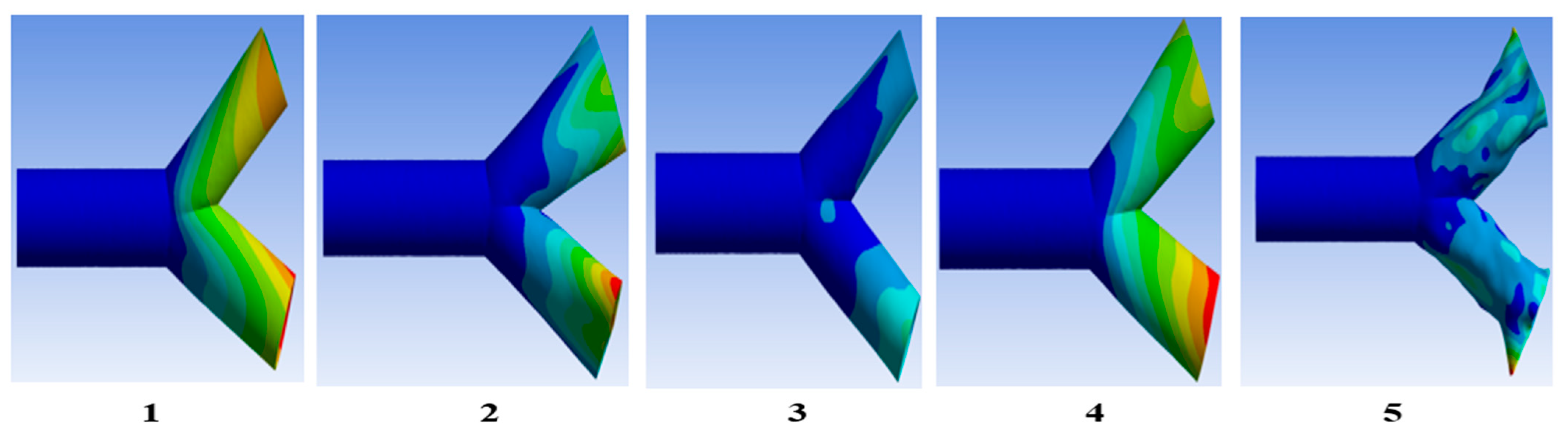
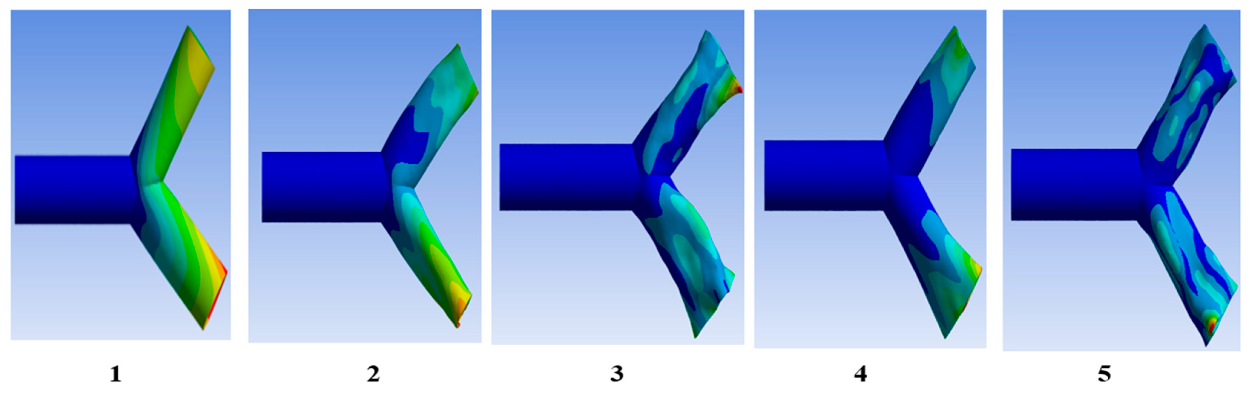
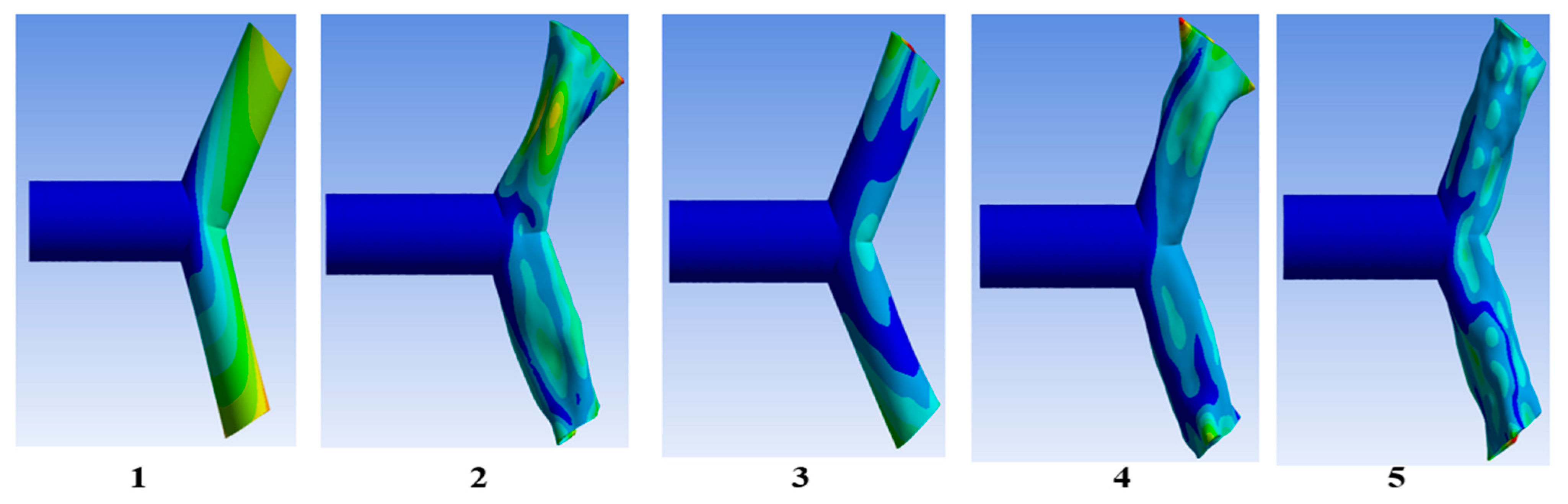
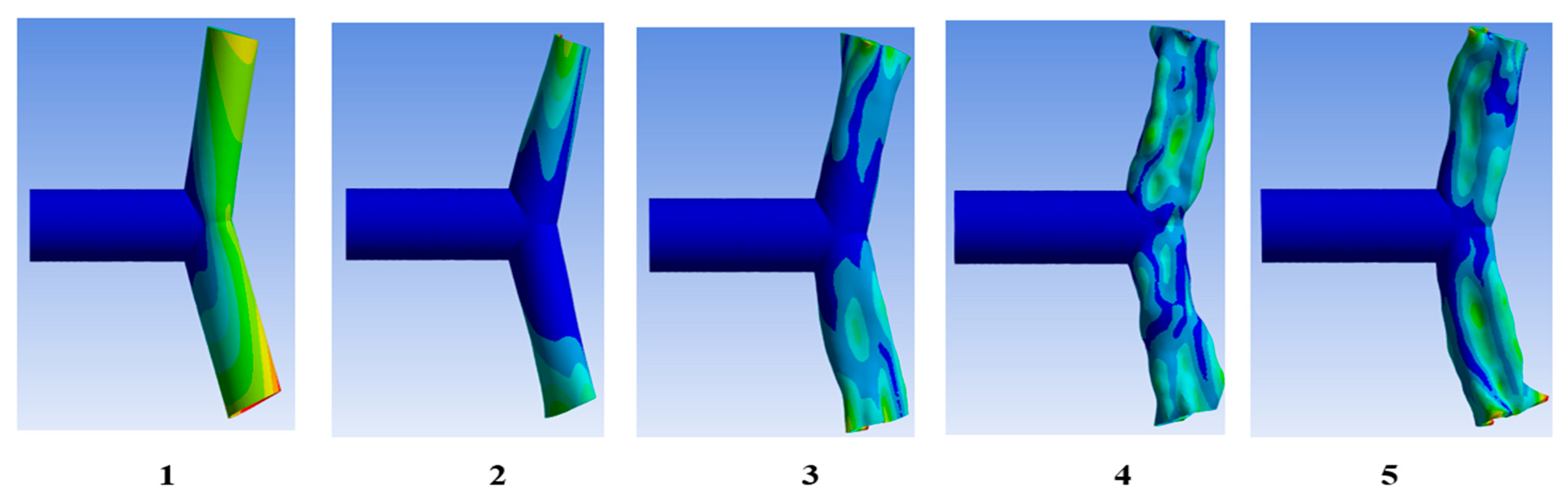
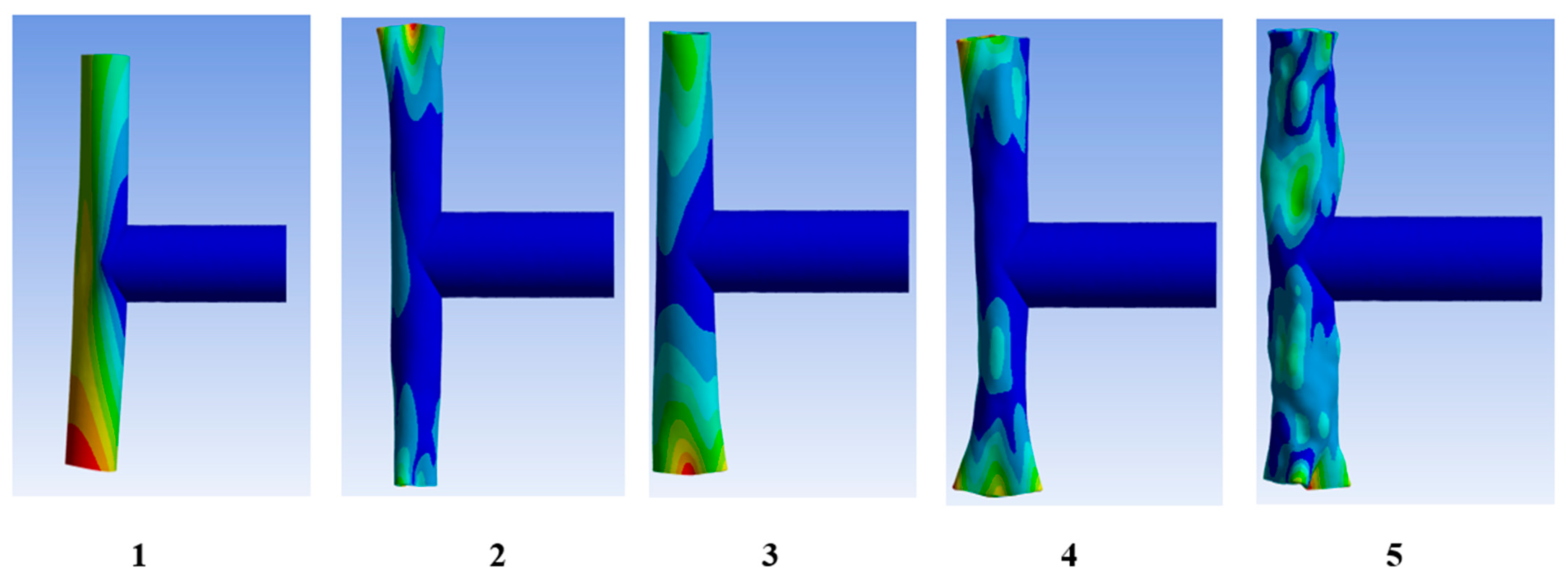
3.3.4. Mode and Mode Shape Analysis

Mode analysis is conducted with remote displacement to represent the pin support of the nanotube. This analysis determines the fundamental frequency per mode shape of CNT. The mode shapes and fundamental frequencies are essential for understanding the vibrational characteristics of the CNT. The vibrational frequency for 10 modes was obtained with the corresponding deformation for each of the modes shaped. In the analysis of random vibration, these parameters are key to determining the PSD values, which help in describing the variation of vibrational energy. The setup for the modal analysis is explained as follows:

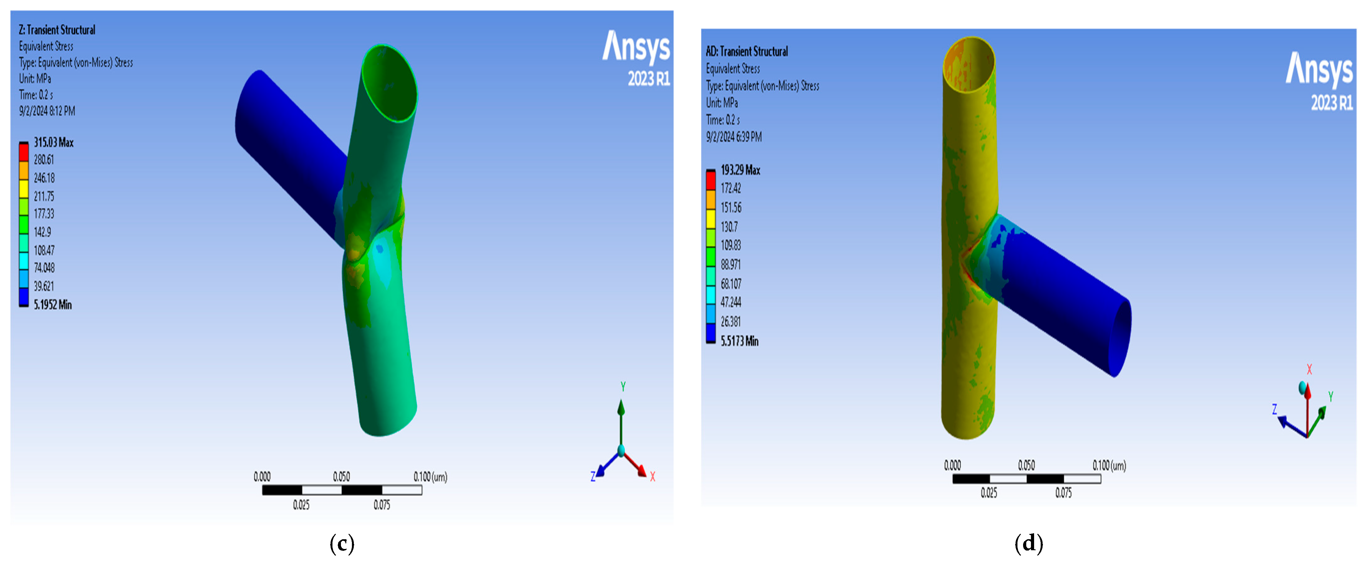
3.3.5. Transient Structural Analysis

The transient structural analysis is used to simulate the overall effect of varying forces on the nanotube under elastic conditions. An elastic support with a stiffness constant of 0.0000003 N/mm².

Cylindrical support is imposed on the tube. The magnetostatic force obtained from the magnetostatic analysis is imported using Ansys MAPDL scripts to account for the effect of magnetism. The transient structural analysis was run for 2 steps within 1 s. The initial time step was set at 0.01 s, with the maximum and minimum time steps at 0.01 s and 0.001 s, respectively.

3.3.6. Grid Independence Test

To make sure that the mesh size has no discernible impact on the simulation results, a grid independence test is conducted. This test involves changing the parameters and comparing the outcomes to ensure consistency. To ensure that the mesh size selected yields dependable results without needless computational overhead, the grid independence test data validates the viability and accuracy of the results for the straight CNTs.

3.3.7. Data Collection

The results obtained from the simulations were stored in formats compatible with the subsequent machine learning stages. Specifically, image outputs, such as mode shapes, stress contour maps, and bifurcation diagrams, were saved in JPEG and PNG formats. Numerical data, including displacement magnitudes, natural frequencies, and other feature values, were exported and stored in CSV (comma-separated values) format to facilitate preprocessing, feature extraction, and training of the machine learning models.

The collected data include mode shapes, natural frequencies, stress distributions, and displacement patterns, which are crucial for a comprehensive understanding of the vibrational behavior of CNTs.

The dataset shape of the dataset is 121 rows with 36 columns representing various physical measurements and conditions.

3.3.8. Data Preparation

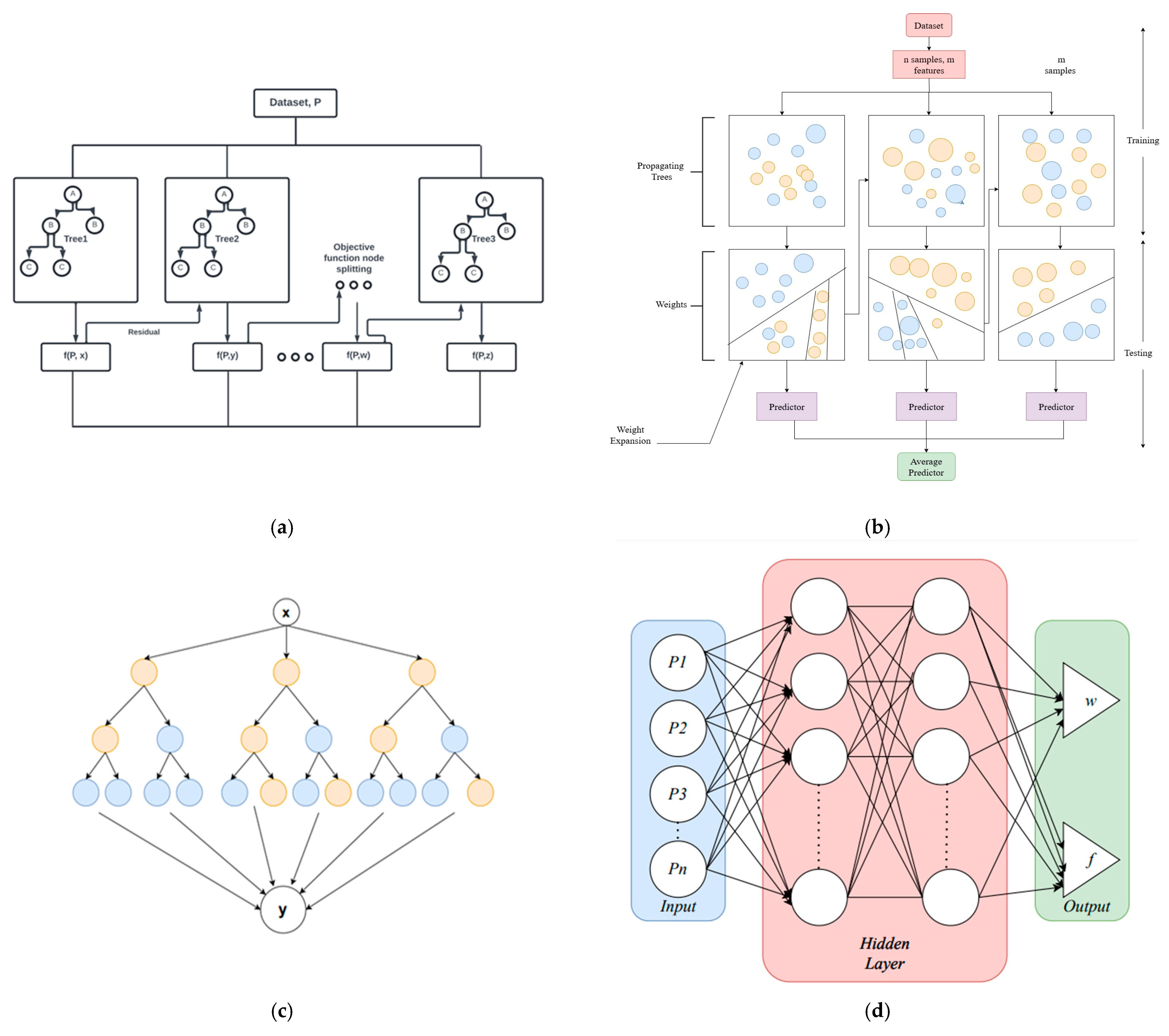
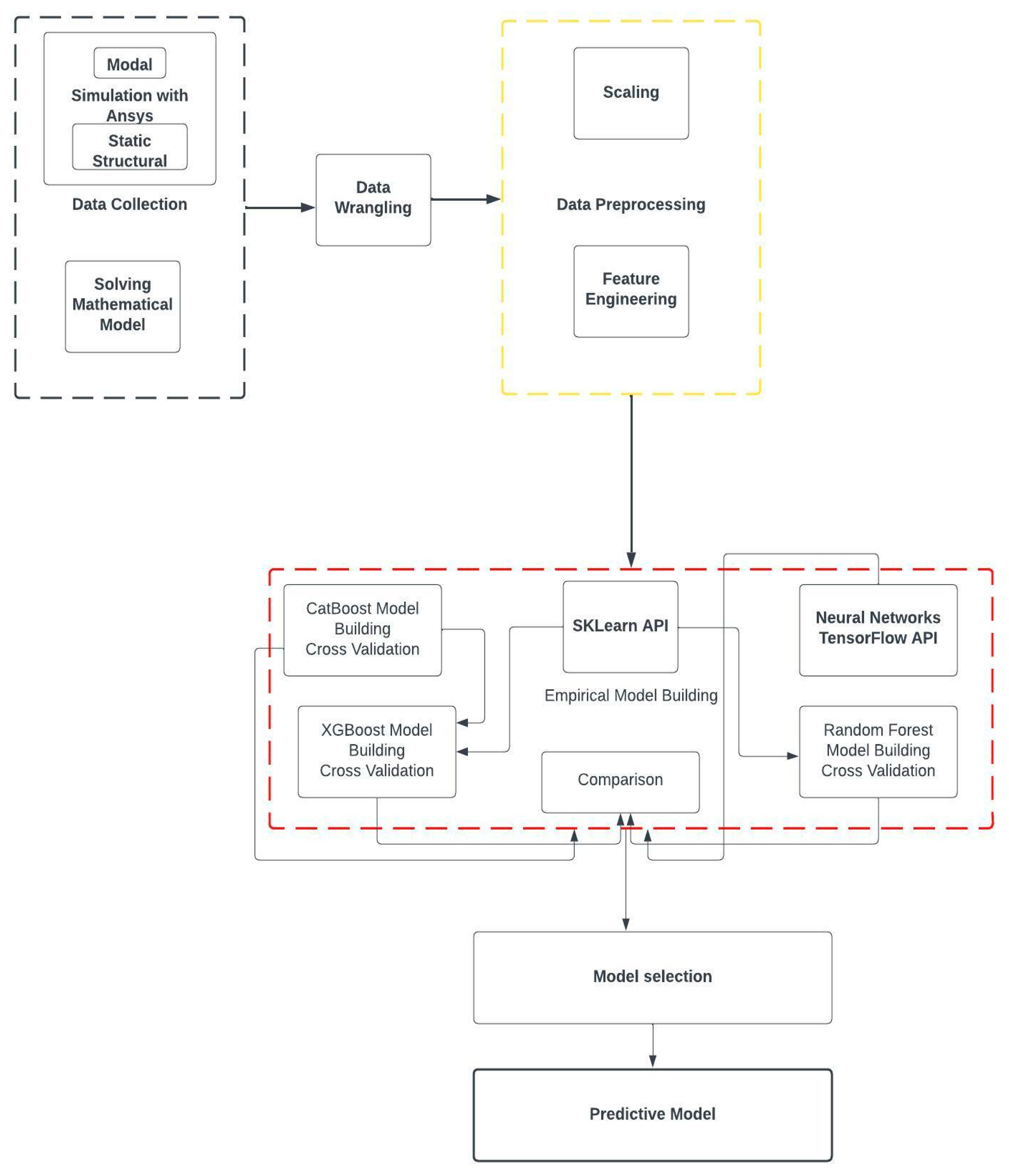
Before model building, the data was carefully preprocessed. Missing values were detected and processed using linear interpolation in a bid to maintain dataset integrity without bias. Statistical tests were used to detect outliers, which were corrected or removed based on physical reasonableness. Feature variables were scaled using the StandardScaler method in a way that each variable’s mean was zero and its standard deviation was one, thus boosting model convergence and performance.

The data preparation process for building the machine learning models is as follows:

Data Cleaning: The dataset was inspected for null values, outliers, and inconsistencies. An interpolation technique was used to fill in any missing data, ensuring that the dataset was complete and ready for modeling. The columns were renamed to simpler, more descriptive names, facilitating easier analysis and interpretation.

Exploratory Data Analysis (EDA): Exploratory data analysis was performed to understand the data. Histograms are plotted for each of the features to understand the distribution of the features. About 68% of the features depict a Gaussian distribution (normal distribution). Also, the correlation plot shows that most of the features are correlated. However, the stability frequency and the mass coefficient are highly correlated.

Scaling and Normalization: The feature distributions were analyzed and found to be approximately Gaussian for about 68% of the features, which justified the application of StandardScaler to normalize the dataset effectively before model training. Features were standardized using StandardScaler to ensure that all input variables had similar scales, improving the performance of machine learning algorithms.

Data Splitting: After preprocessing, the dataset was randomly shuffled and split into training and testing sets in a 4:1 ratio (80% training, 20% testing). This split ensured that the models could be trained on most of the data at hand while being validated on an unseen subset to evaluate generalizability. No data leakage occurred between training and test sets. These preprocessing steps were implemented using Python libraries, including Pandas (version 2.1.4) and Scikit-learn (version 1.4.2). Being a supervised learning process, the key input parameters are shown in

Table 4. Summary of key input parameters used in simulation.

Parameter	Symbol	Value Range	Units
Magnetic Field Strength	B	50–150	mT
Axial Flow Velocity	U	0–300	m/s
Nanotube Diameter	D	30	nm
Nanotube Wall Thickness	t	1	nm
Young’s Modulus	E	3.6	TPa
Density of Nanotube Material	Ρ	1330	kg/m3
Magnetic Permeability	Μ	1.05	-
Winkler Foundation Stiffness	kw	3 × 10−7	N/mm2
Branching Angle	Φ	0–90°	Degrees
Thermal Environment Temperature	T	300–400	K

.

3.4. Model Building

The model-building process is presented in Figure 4. Four different machine learning models were chosen to predict the displacement and frequency of each mode. These are XGBoost, CATBoost, Random Forest, and Neural Network.

XGBoost: The model is configured with hyperparameters such as learning rate, max depth, and number of estimators. These parameters control the complexity and learning process of the model. The model is trained using the training dataset. Common to the XGBoost algorithm is the utilization of gradient boosting techniques to minimize prediction error, which enhance the possibility of generating more accurate results.

Mathematically, we can observe the objective of the XGBoost algorithm as that which would always try to reduce the loss function and a regularization term.

$$\mathcal{L}(y,\widehat{y})={\displaystyle \sum _{i=1}^n{L}_a}(y_i,{\widehat{y}}_i)+{\Omega }_{XGB}(F)$$

(105)

The regularization term which is a composition of L1 and L2 is given by the following:

$${\Omega }_{XGB}(F)={\gamma }_L{T}_n+{\displaystyle \frac{1}{2}}{\lambda }_j{\displaystyle \sum _{i=1}^T{\displaystyle \sum _{j=1}^d{(w_{ij})}^2}}$$

(106)

Due to the iterative nature of the XGBoost algorithm, the i-th instance of the predicted value can be given as follows:

$${\widehat{y}}_i^{(t)}={\widehat{y}}_i^{(t-1)}+f_t(x_i)$$

(107)

CATBoost: CATBoost is set up with parameters like XGBoost, including learning rate, depth, and number of iterations. CATBoost is particularly effective with categorical features, but here we focus on numerical features. The model is trained with the training data, leveraging its boosting capabilities to handle overfitting and improve prediction accuracy.

$$\mathcal{L}(y,\widehat{y})={\displaystyle \sum _{i=1}^{n}L}(y_i,{\widehat{y}}_i)+{\Omega }_{CAT}(F)$$

(108)

The regularization term is like that of XGBoost, and as such, can be represented by Equation (106). While the loss function is similar, it is worth noting that the way categorical features are handled by each algorithm differs.

Random Forest: Random Forest is configured with parameters such as the number of trees and maximum depth. This model creates an ensemble of decision trees to make predictions. This model is trained by aggregating the predictions from multiple decision trees to reduce variance and improve robustness.

Where a Random Forest can be denoted as F, the predictions for a new instance may be defined as follows:

$$F(x)={\displaystyle \frac{1}{n_i}}{\displaystyle \sum _{n_i=1}^{n_i}{T}_b}(x)$$

(109)

Neural Network: The neural network architecture includes several dense layers with activation functions such as ReLU. Dropout layers are used to prevent overfitting. The model is trained with a specified number of epochs and a validation split to monitor performance. Early stopping is employed to halt training when no further improvement is observed, preventing overfitting.

Evaluation: Performance of each model is evaluated using metrics such as Mean Squared Error (MSE) and R². These metrics provide insight into how well the model predictions match the actual values. For models like XGBoost, CATBoost, and Random Forest, feature importance is computed to understand which features contribute the most to the predictions. This helps in identifying key factors affecting vibration modes. Therefore, we then obtain the displacement w(x,t) by combining the special term obtained from the boundary condition and the temporal term obtained from after treatment.

4. Results and Discussion

4.1. Results from Mathematical Modeling

The following outcomes are attained by focusing on the problem’s physics and carrying out sufficient parametric research.

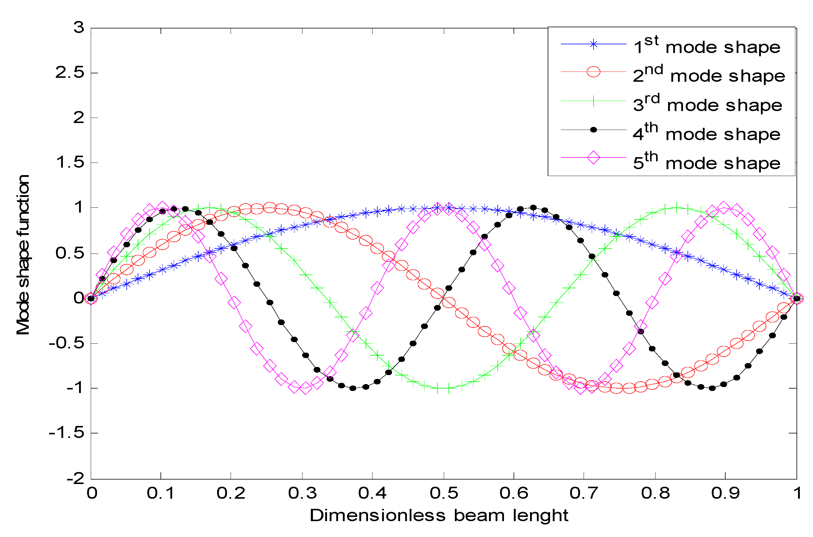
4.1.1. Modal Numbers’ Impact on Nanotube’s Mode Shapes

Figure 5 shows how the boundary conditions and mode number affect the nanotube’s nonlinear deformation patterns. For the first five mode configurations, this graphic displays the deflection of the nanotube along its dimensionless length. We can see from this image that for a given beam length, the stability of the nanotube decreases as the mode number upsurges. This behavior is explained by the trial function’s reliance on the mode number.

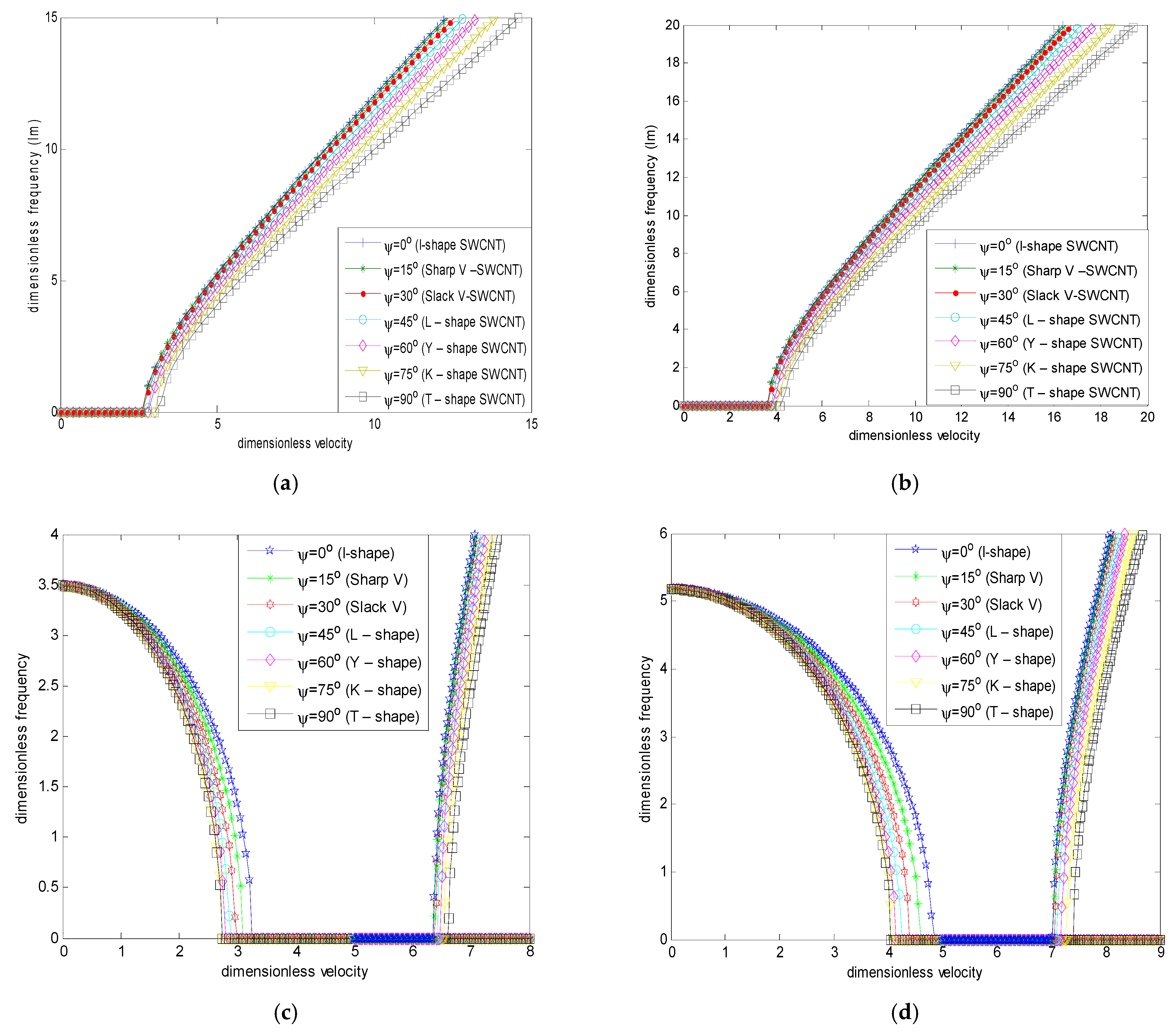
4.1.2. Branch Angles’ Impacts on Stability

The relationship between dimensionless frequency and dimensionless flow velocity is shown to be influenced by the downstream angle, which establishes the end shape of the nanotube (Figure 6 and Figure 7). With increasing velocity, the frequency first falls parabolically for both linear and nonlinear foundations. This suggests that within this range, the nanotube stays stable. Nevertheless, the nanotube eventually reaches a critical dimensionless velocity, after which bifurcation makes it unstable. This suggests that the nanotube is more stable under nonlinear conditions. Furthermore, the region of bifurcation is shorter for the nonlinear analysis, meaning that the nanotube regains stability more quickly after becoming unstable. As the flow velocity continues to increase beyond the critical velocity, the system remains unstable with zero frequency. Eventually, another critical velocity is reached where the system temporarily stabilizes. However, further increases in velocity can lead to divergence and potentially flutter.

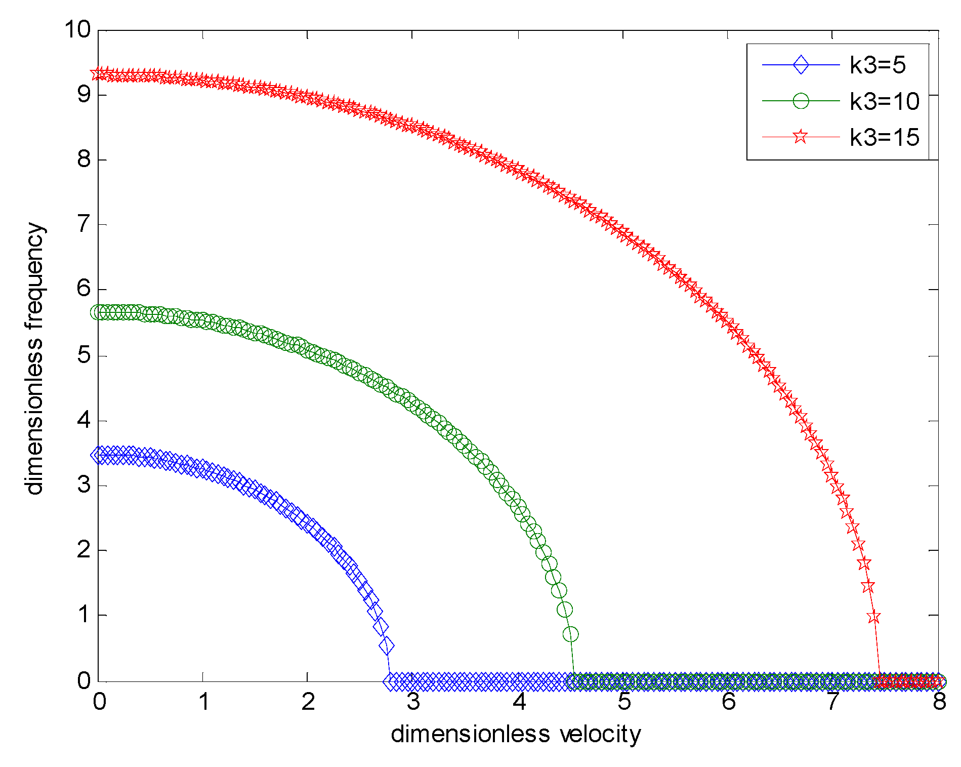
4.1.3. Winkler’s Foundations Effects on Stability of SWCNT

Figure 8 shows how the foundation affects the stability of the nanotube. The graphs show that raising the Winkler foundation coefficients causes the stiffness of the nanotube to grow in tandem, raising the system frequencies.

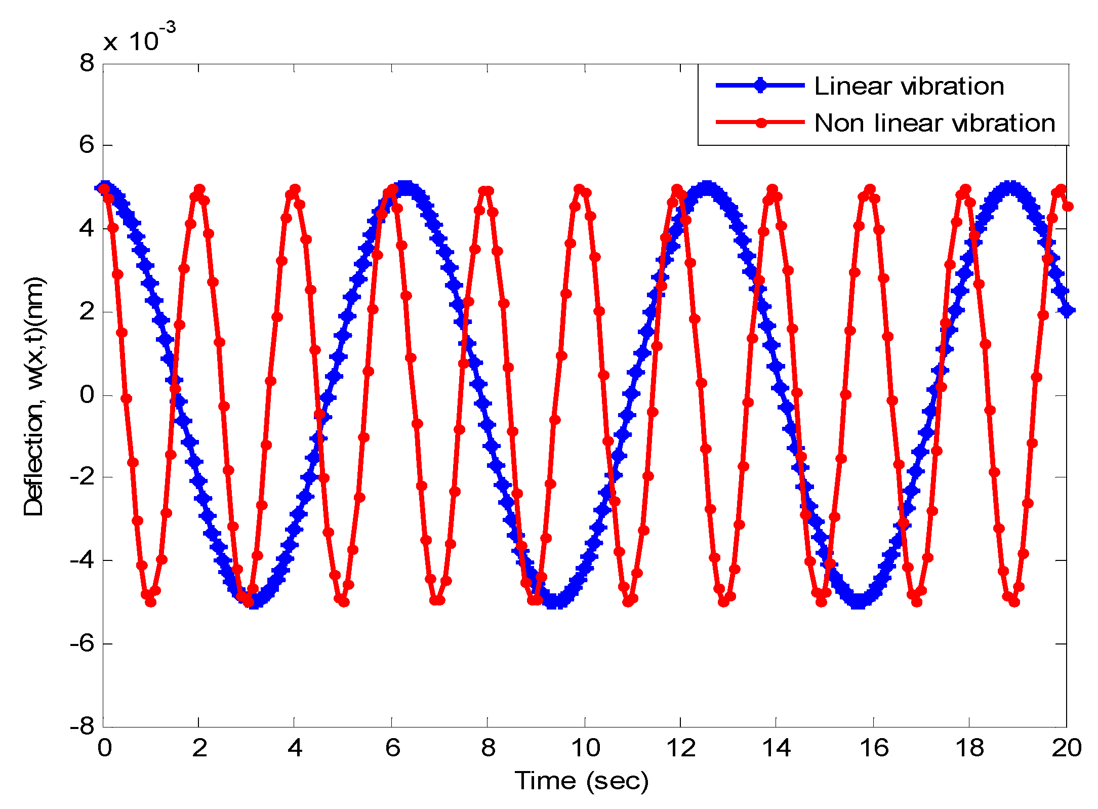
4.1.4. Vibrational Dynamic Responses of the SWCNT

The carbon nanotube’s nonlinear and linear dynamics are contrasted in Figure 9. The divergence is caused by the nonlinear variables present in the Duffing equations, which are used to compute nonlinear frequency and frequency ratio. As the maximal dynamic vibration rises, this difference becomes more noticeable.

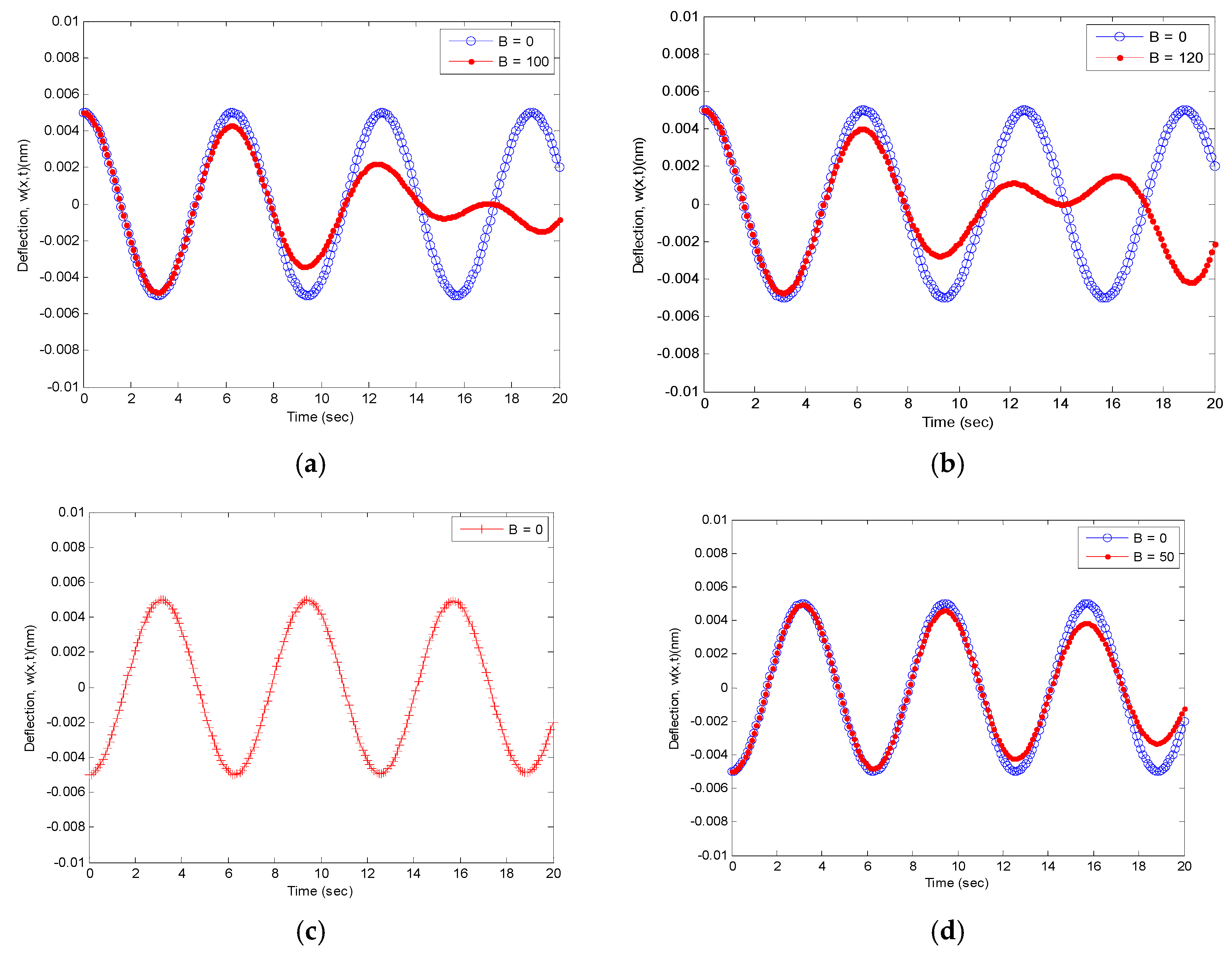
4.1.5. Magnetic Term’s Influence on SWCNT Response

The influences of the magnetic term on dynamic responses of the nanotube for modes 1 and 2 are shown in Figure 10a–d. It was discovered that mode 2 responses were completely out of sync with the mode 1 responses. Furthermore, it was found that as the magnetic influence grew, the system’s dynamic responses decreased. This suggests that the dynamic activity of the nanotube is dampened by the magnetic characteristic.

4.2. Simulation Results

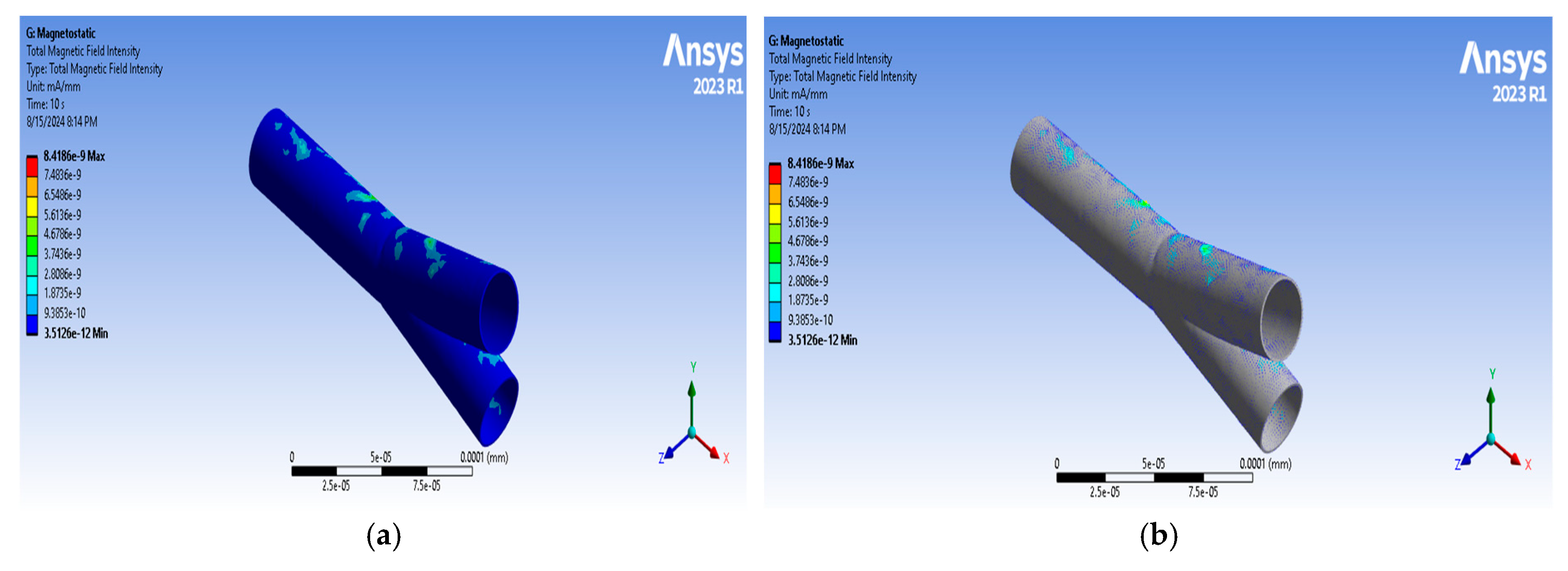
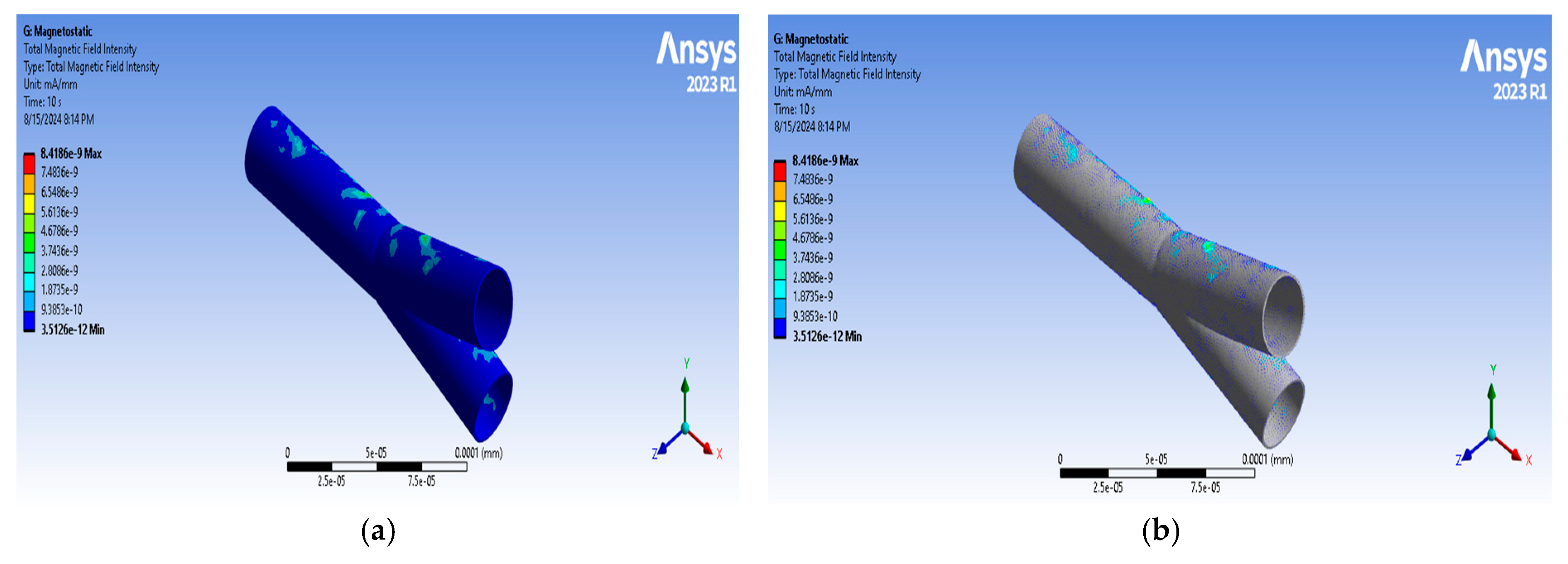
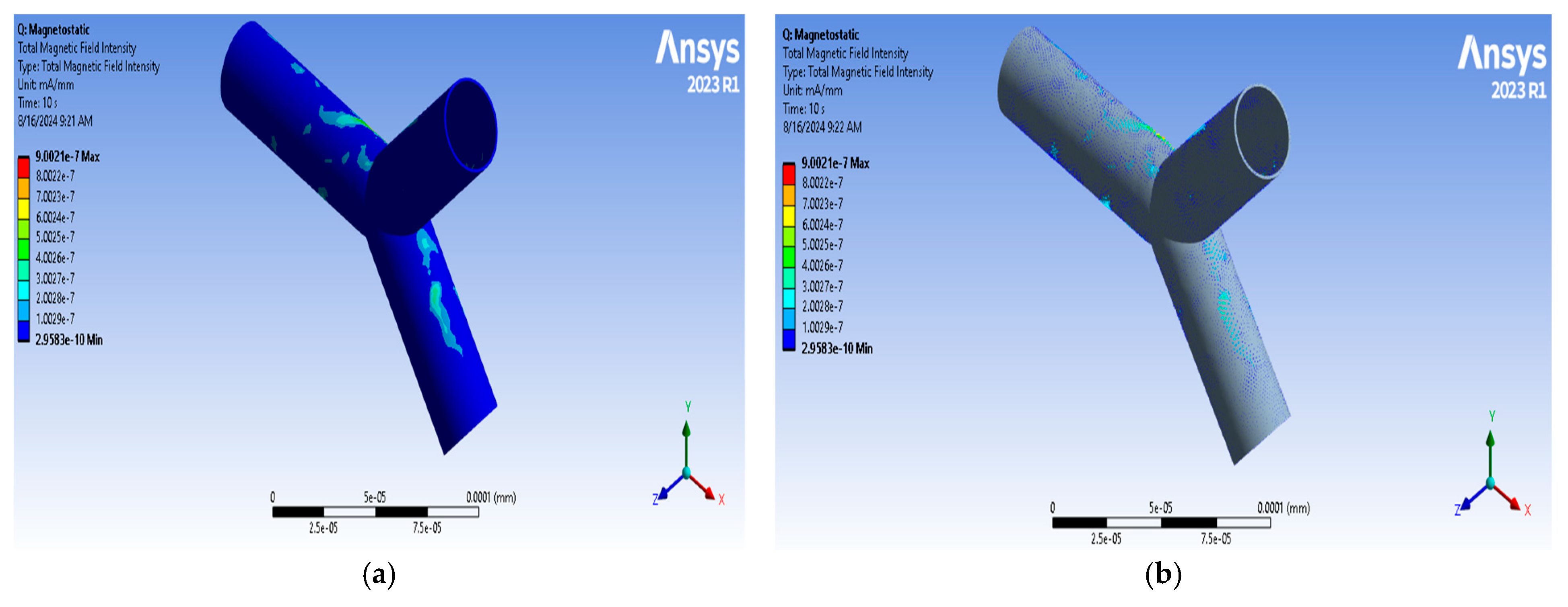
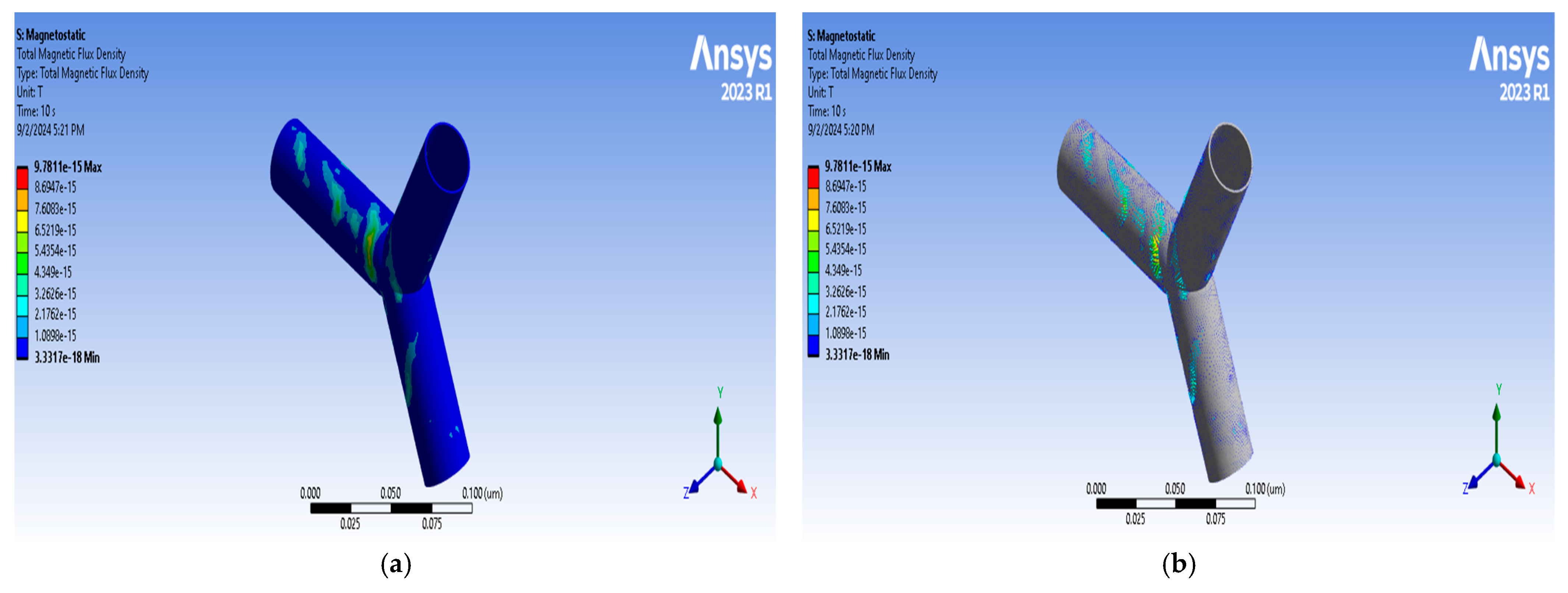
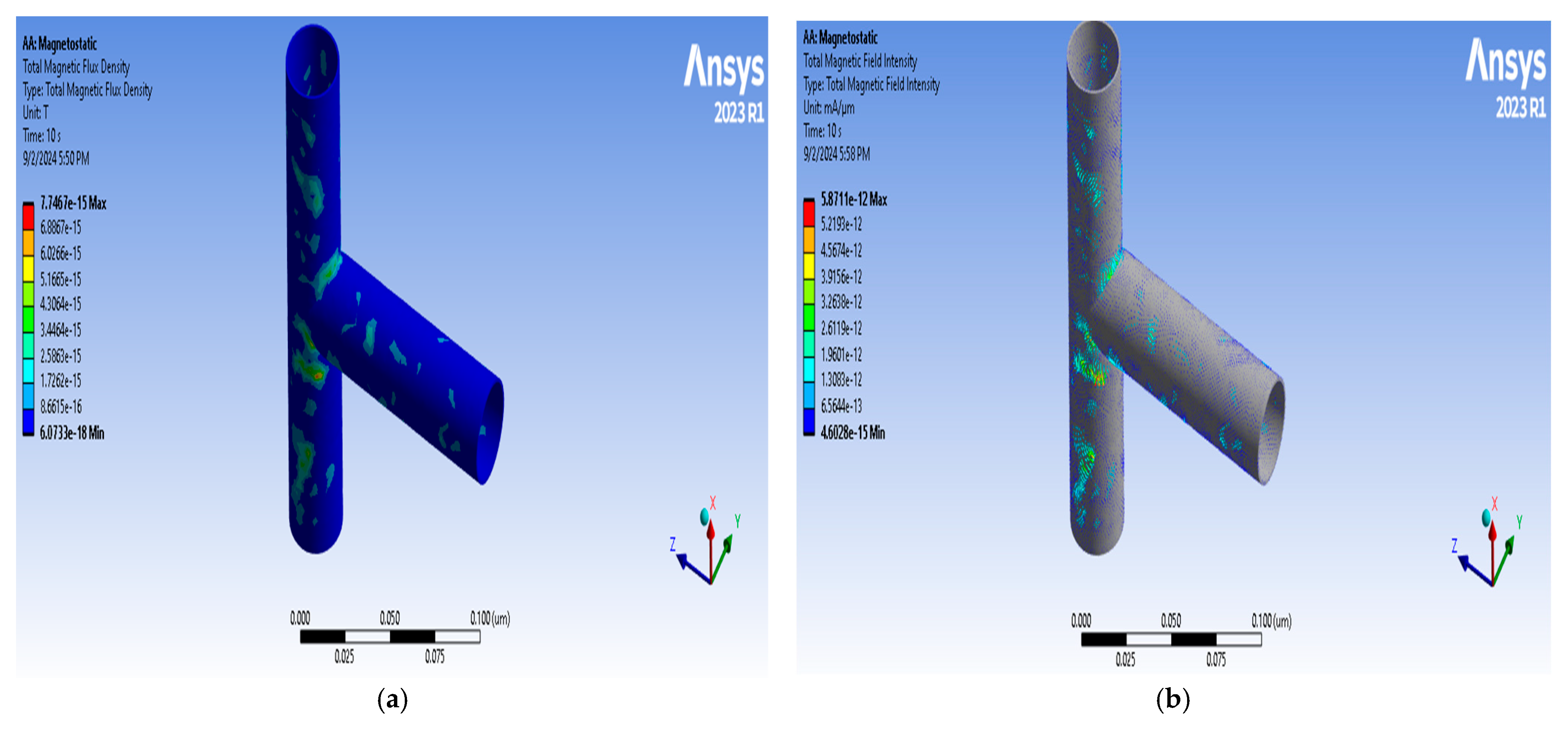
4.2.1. Magnetostatic Analysis

The magnetic flux density (MFD) and magnetic flux intensity (MFI) vary along the periphery of the straight nanotube and are even more evident in the surface area, as shown in Figure 11 and

Table 5. MFD and MFI for I-shaped nanotube.

Time Steps	MiMFD (mT)	MaMFD (mT)	AvMFD (mT)	MiMFI (mA/mm)	MaMFI (mA/mm)	AvMFI (mA/mm)
1.	0	0	0	0	0	0
2.	5.1727 × 10−4	6.9473 × 10−2	2.9487 × 10−2	4.1163 × 10−5	5.5285 × 10−3	2.3465 × 10−3
3.	5.8193 × 10−4	7.8157 × 10−2	3.3173 × 10−2	4.6309 × 10−5	6.2195 × 10−3	2.6398 × 10−3
4.	6.4659 × 10−4	8.6841 × 10−2	3.6858 × 10−2	5.1454 × 10−5	6.9106 × 10−3	2.9331 × 10−3
5.	7.1125 × 10−4	9.5525 × 10−2	4.0544 × 10−2	5.66 × 10−5	7.6016 × 10−3	3.2264 × 10−3
6.	7.7591 × 10−4	0.10421	4.423 × 10−2	6.1745 × 10−5	8.2927 × 10−3	3.5197 × 10−3
7.	9.0523 × 10−4	0.12158	5.1602 × 10−2	7.2036 × 10−5	9.6748 × 10−3	4.1063 × 10−3
8.	9.9144 × 10−4	0.13316	5.6516 × 10−2	7.8896 × 10−5	1.0596 × 10−2	4.4974 × 10−3
9.	1.0777 × 10−3	0.14473	6.1431 × 10−2	8.5757 × 10−5	1.1518 × 10−2	4.8885 × 10−3
10.	1.1639 × 10−3	0.15631	6.6345 × 10−2	9.2618 × 10−5	1.2439 × 10−2	5.2796 × 10−3

presents the actual values.

The magnetic flux density and magnetic flux intensity for Y-shaped and T-shaped nanotubes exhibit a contrasting behavior to those seen in the straight nanotube, as they are almost uniform across the surface with slight areas having relatively higher values, as shown in Figure 12, Figure 13, Figure 14, Figure 15, Figure 16 and Figure 17 and

Table 6. MFD and MFI of nanotube with branch angle of 15°.

Time Steps	MiMFD (mT)	MaMFD (mT)	AvMFD (mT)	MiMFI (mA/mm)	MaMFI (mA/mm)	AvMFI (mA/mm)
1.	4.414 × 10−12	1.0579 × 10−8	4.922 × 10−10	3.5126 × 10−13	8.4186 × 10−10	3.9168 × 10−11
2.	1.1035 × 10−11	2.6448 × 10−8	1.2305 × 10−9	8.7814 × 10−13	2.1047 × 10−9	9.792 × 10−11
3.	1.7215 × 10−11	4.1259 × 10−8	1.9196 × 10−9	1.3699 × 10−12	3.2833 × 10−9	1.5275 × 10−10
4.	1.7656 × 10−11	4.2317 × 10−8	1.9688 × 10−9	1.405 × 10−12	3.3675 × 10−9	1.5667 × 10−10
5.	2.4277 × 10−11	5.8185 × 10−8	2.7071 × 10−9	1.9319 × 10−12	4.6303 × 10−9	2.1542 × 10−10
6.	2.8691 × 10−11	6.8765 × 10−8	3.1993 × 10−9	2.2832 × 10−12	5.4721 × 10−9	2.5459 × 10−10
7.	3.0898 × 10−11	7.4054 × 10−8	3.4454 × 10−9	2.4588 × 10−12	5.893 × 10−9	2.7417 × 10−10
8.	3.5312 × 10−11	8.4633 × 10−8	3.9376 × 10−9	2.81 × 10−12	6.7349 × 10−9	3.1334 × 10−10
9.	3.9726 × 10−11	9.5213 × 10−8	4.4298 × 10−9	3.1613 × 10−12	7.5768 × 10−9	3.5251 × 10−10
10.	4.414 × 10−11	1.0579 × 10−7	4.922 × 10−9	3.5126 × 10−12	8.4186 × 10−9	3.9168 × 10−10

,

Table 7. MFD and MFI of nanotube with branch angle of 30°.

Time Steps	MiMFD (mT)	MaMFD (mT)	AvMFD (mT)	MiMFI (mA/mm)	MaMFI (mA/mm)	AvMFI (mA/mm)
1.	9.4821 × 10−13	3.5836 × 10−9	2.3093 × 10−10	7.5456 × 10−14	2.8517 × 10−10	1.8377 × 10−11
2.	2.95 × 10−12	1.1149 × 10−8	7.1844 × 10−10	2.3475 × 10−13	8.8721 × 10−10	5.7172 × 10−11
3.	4.9518 × 10−12	1.8714 × 10−8	1.206 × 10−9	3.9405 × 10−13	1.4892 × 10−9	9.5967 × 10−11
4.	6.9535 × 10−12	2.628 × 10−8	1.6935 × 10−9	5.5334 × 10−13	2.0913 × 10−9	1.3476 × 10−10
5.	8.9553 × 10−12	3.3845 × 10−8	2.181 × 10−9	7.1264 × 10−13	2.6933 × 10−9	1.7356 × 10−10
6.	1.0957 × 10−11	4.1411 × 10−8	2.6685 × 10−9	8.7194 × 10−13	3.2954 × 10−9	2.1235 × 10−10
7.	1.2959 × 10−11	4.8976 × 10−8	3.156 × 10−9	1.0312 × 10−12	3.8974 × 10−9	2.5115 × 10−10
8.	1.4961 × 10−11	5.6541 × 10−8	3.6435 × 10−9	1.1905 × 10−12	4.4994 × 10−9	2.8994 × 10−10
9.	1.6962 × 10−11	6.4107 × 10−8	4.131 × 10−9	1.3498 × 10−12	5.1015 × 10−9	3.2874 × 10−10
10.	1.8964 × 10−11	7.1672 × 10−8	4.6185 × 10−9	1.5091 × 10−12	5.7035 × 10−9	3.6753 × 10−10

,

Table 8. MFD and MFI of nanotube with branch angle of 45°.

Time Steps	MiMFD (mT)	MaMFD (mT)	AvMFD (mT)	MiMFI (mA/mm)	MaMFI (mA/mm)	AvMFI (mA/mm)
1.	3.3458 × 10−10	1.0181 × 10−6	4.7945 × 10−8	2.6625 × 10−11	8.1019 × 10−8	3.8153 × 10−9
2.	7.1046 × 10−10	2.1619 × 10−6	1.0181 × 10−7	5.6537 × 10−11	1.7204 × 10−7	8.1017 × 10−9
3.	1.0863 × 10−9	3.3057 × 10−6	1.5567 × 10−7	8.6449 × 10−11	2.6306 × 10−7	1.2388 × 10−8
4.	1.4622 × 10−9	4.4496 × 10−6	2.0954 × 10−7	1.1636 × 10−10	3.5408 × 10−7	1.6674 × 10−8
5.	1.8381 × 10−9	5.5934 × 10−6	2.634 × 10−7	1.4627 × 10−10	4.4511 × 10−7	2.0961 × 10−8
6.	2.214 × 10−9	6.7372 × 10−6	3.1727 × 10−7	1.7618 × 10−10	5.3613 × 10−7	2.5247 × 10−8
7.	2.5899 × 10−9	7.881 × 10−6	3.7113 × 10−7	2.061 × 10−10	6.2715 × 10−7	2.9534 × 10−8
8.	2.9658 × 10−9	9.0248 × 10−6	4.2499 × 10−7	2.3601 × 10−10	7.1817 × 10−7	3.382 × 10−8
9.	3.3417 × 10−9	1.0169 × 10−5	4.7886 × 10−7	2.6592 × 10−10	8.0919 × 10−7	3.8106 × 10−8
10.	3.7175 × 10−9	1.1312 × 10−5	5.3272 × 10−7	2.9583 × 10−10	9.0021 × 10−7	4.2393 × 10−8

,

Table 9. MFD and MFI of nanotube with branch angle of 60°.

Time Steps	MiMFD (mT)	MaMFD (mT)	AvMFD (mT)	MiMFI (mA/mm)	MaMFI (mA/mm)	AvMFI (mA/mm)
1.	3.3317 × 10−19	9.7811 × 10−16	4.5868 × 10−17	2.525 × 10−16	7.4129 × 10−13	3.4763 × 10−14
2.	6.6633 × 10−19	1.9562 × 10−15	9.1737 × 10−17	5.05 × 10−16	1.4826 × 10−12	6.9525 × 10−14
3.	9.995 × 10−19	2.9343 × 10−15	1.376 × 10−16	7.575 × 10−16	2.2239 × 10−12	1.0429 × 10−13
4.	1.3327 × 10−18	3.9125 × 10−15	1.8347 × 10−16	1.01 × 10−15	2.9652 × 10−12	1.3905 × 10−13
5.	1.6658 × 10−18	4.8906 × 10−15	2.2934 × 10−16	1.2625 × 10−15	3.7065 × 10−12	1.7381 × 10−13
6.	1.999 × 10−18	5.8687 × 10−15	2.7521 × 10−16	1.515 × 10−15	4.4478 × 10−12	2.0858 × 10−13
7.	2.3322 × 10−18	6.8468 × 10−15	3.2108 × 10−16	1.7675 × 10−15	5.1891 × 10−12	2.4334 × 10−13
8.	2.6653 × 10−18	7.8249 × 10−15	3.6695 × 10−16	2.02 × 10−15	5.9304 × 10−12	2.781 × 10−13
9.	2.9985 × 10−18	8.803 × 10−15	4.1281 × 10−16	2.2725 × 10−15	6.6716 × 10−12	3.1286 × 10−13
10.	3.3317 × 10−18	9.7811 × 10−15	4.5868 × 10−16	2.525 × 10−15	7.4129 × 10−12	3.4763 × 10−13

,

Table 10. MFD and MFI of nanotube with branch angle of 75°.

Time Steps	MiMFD (mT)	MaMFD (mT)	AvMFD (mT)	MiMFI (mA/mm)	MaMFI (mA/mm)	AvMFI (mA/mm)
1.	4.0206 × 10−19	1.1934 × 10−15	3.3235 × 10−17	3.0472 × 10−16	9.0442 × 10−13	2.5188 × 10−14
2.	8.0412 × 10−19	2.3867 × 10−15	6.647 × 10−17	6.0943 × 10−16	1.8088 × 10−12	5.0376 × 10−14
3.	1.2062 × 10−18	3.5801 × 10−15	9.9705 × 10−17	9.1415 × 10−16	2.7133 × 10−12	7.5565 × 10−14
4.	1.6082 × 10−18	4.7734 × 10−15	1.3294 × 10−16	1.2189 × 10−15	3.6177 × 10−12	1.0075 × 10−13
5.	2.0103 × 10−18	5.9668 × 10−15	1.6618 × 10−16	1.5236 × 10−15	4.5221 × 10−12	1.2594 × 10−13
6.	2.4124 × 10−18	7.1601 × 10−15	1.9941 × 10−16	1.8283 × 10−15	5.4265 × 10−12	1.5113 × 10−13
7.	2.8144 × 10−18	8.3535 × 10−15	2.3265 × 10−16	2.133 × 10−15	6.331 × 10−12	1.7632 × 10−13
8.	3.2165 × 10−18	9.5469 × 10−15	2.6588 × 10−16	2.4377 × 10−15	7.2354 × 10−12	2.0151 × 10−13
9.	3.6186 × 10−18	1.074 × 10−14	2.9912 × 10−16	2.7424 × 10−15	8.1398 × 10−12	2.2669 × 10−13
10.	4.0206 × 10−18	1.1934 × 10−14	3.3235 × 10−16	3.0472 × 10−15	9.0442 × 10−12	2.5188 × 10−13

and

Table 11. MFD and MFI of nanotube with branch angle of 90°.

Time Steps	MiMFD (mT)	MaMFD (mT)	AvMFD (mT)	MiMFI (mA/mm)	MaMFI (mA/mm)	AvMFI (mA/mm)
1.	6.0733 × 10−19	7.7467 × 10−16	4.8008 × 10−17	4.6028 × 10−16	5.8711 × 10−13	3.6384 × 10−14
2.	1.2147 × 10−18	1.5493 × 10−15	9.6016 × 10−17	9.2056 × 10−16	1.1742 × 10−12	7.2768 × 10−14
3.	1.822 × 10−18	2.324 × 10−15	1.4402 × 10−16	1.3808 × 10−15	1.7613 × 10−12	1.0915 × 10−13
4.	2.4293 × 10−18	3.0987 × 10−15	1.9203 × 10−16	1.8411 × 10−15	2.3484 × 10−12	1.4554 × 10−13
5.	3.0366 × 10−18	3.8734 × 10−15	2.4004 × 10−16	2.3014 × 10−15	2.9355 × 10−12	1.8192 × 10−13
6.	3.644 × 10−18	4.648 × 10−15	2.8805 × 10−16	2.7617 × 10−15	3.5227 × 10−12	2.1831 × 10−13
7.	4.2513 × 10−18	5.4227 × 10−15	3.3606 × 10−16	3.222 × 10−15	4.1098 × 10−12	2.5469 × 10−13
8.	4.8586 × 10−18	6.1974 × 10−15	3.8406 × 10−16	3.6823 × 10−15	4.6969 × 10−12	2.9107 × 10−13
9.	5.466 × 10−18	6.9721 × 10−15	4.3207 × 10−16	4.1425 × 10−15	5.284 × 10−12	3.2746 × 10−13
10.	6.0733 × 10−18	7.7467 × 10−15	4.8008 × 10−16	4.6028 × 10−15	5.8711 × 10−12	3.6384 × 10−13

present the actual values.

4.2.2. Modal Analysis

The modal deformation for different modes is presented below for the different orientations of nanotubes considered in this study. The straight carbon nanotubes consist of two cases, which were when there were simple supports at both ends and with and without support on the external surface area of the cylinder.

The modal shapes with the deformation at different modes for I-shaped CNT are presented as follows:

Figure 18 and Figure 19 both represent the deformation at different modes. The deformation is seen to increase steadily for the first five modes.

The modal shapes with the deformation at different modes for Y-shaped CNT are presented in

Table 12. Modal frequency for CNT at varying downstream angle.

	Frequency (MHz)
Modes	0	15	30	45	60	75	90
1	2.353 × 10−11	2.08 × 10−12	9.08 × 10−6	2.56 × 10−13	−2.0479 × 10−13	2.0312 × 10−13	4.0616 × 10−13
2	1.5417 × 10−11	3.32 × 10−7	3.33 × 10−6	3.90 × 10−7	−1.061 × 10−9	1.061 × 10−9	1.061 × 10−9
3	1.2398 × 10−10	4.02 × 10−7	3.13 × 10−5	1.47 × 10−7	−1.061 × 10−9	1.061 × 10−9	1.061 × 10−9
4	2.058 × 10−10	3.43 × 10−7	3.19 × 10−5	5.67 × 10−7	−1.061 × 10−9	1.061 × 10−9	1.061 × 10−9
5	2.7809 × 10−10	9.83 × 10−7	4.75 × 10−5	4.52 × 10−7	−1.061 × 10−9	1.061 × 10−9	1.061 × 10−9
6	3.9117 × 10−10	3.70 × 10−7	6.89 × 10−5	7.40 × 10−7	−1.061 × 10−9	1.061 × 10−9	1.061 × 10−9
7	3.9954 × 10−10	1.38 × 10−6	5.18 × 10−5	5.21 × 10−7	−1.061 × 10−9	1.061 × 10−9	1.061 × 10−9
8	4.0446 × 10−10	5.30 × 10−7	6.97 × 10−5	9.04 × 10−7	−1.061 × 10−9	1.061 × 10−9	1.061 × 10−9
9	4.0489 × 10−10	1.82 × 10−6	7.64 × 10−5	1.13 × 10−6	−1.061 × 10−9	1.061 × 10−9	1.061 × 10−9
10	4.0499 × 10−10	6.90 × 10−7	1.52 × 10−4	1.26 × 10−6	−1.061 × 10−9	1.061 × 10−9	1.061 × 10−9

and

Table 13. Deformation for CNT at varying downstream angles.

	Deformation (Ⴏm)
Modes	0	15	30	45	60	75	90
1	31.998	0.00018869	5.72 × 10−5	3.39 × 10−5	9.604 × 10−3	9.2143 × 10−3	8.2562 × 10−3
2	347.69	1.732	2.512	1.6242	1.7744	1.8811	2.2076
3	430.27	1.7666	2.3358	2.1649	1.9492	2.4072	1.8218
4	567.02	1.6772	2.1682	1.9493	2.6251	2.2065	1.8914
5	614.73	1.7843	2.3358	2.3673	2.4339	2.2916	2.2211
6	561.82	1.684	2.1682	2.6993	2.6043	2.1477	1.7175
7	571.76	2.3413	2.3115	1.9122	2.5140	2.4863	1.7255
8	502.72	1.9917	2.2874	2.15218	1.6629	1.8826	1.9705
9	518.4	1.7508	2.1793	2.2192	2.9362	2.1940	1.9857
10	489.92	1.4758	2.2088	1.6817	2.0070	1.1628	1.9993

.

Figure 20, Figure 21, Figure 22, Figure 23, Figure 24 and Figure 25 show large deformations for the branched region of the nanotubes. However, for the T-shaped nanotube, the deformation is prominent along the vertical section, which coincides with the unconstrained section. Figure 25 shows that for all five modes represented, there are large deflections from the branched part of the nanotubes.

4.2.3. Transient Structural Analysis

Figure 26a–d represents the result obtained from the transient structural analysis. For the simply supported I-shaped nanotube, it is observed that there is large radial deformation under the modeled thermo-magnetic environment. Furthermore, for the branched nanotubes, large stress occurs at unsupported edges, with the T-shaped nanotube an exception to this. Maximum stress for the T-shaped nanotube occurs at the inner walls of the tube.

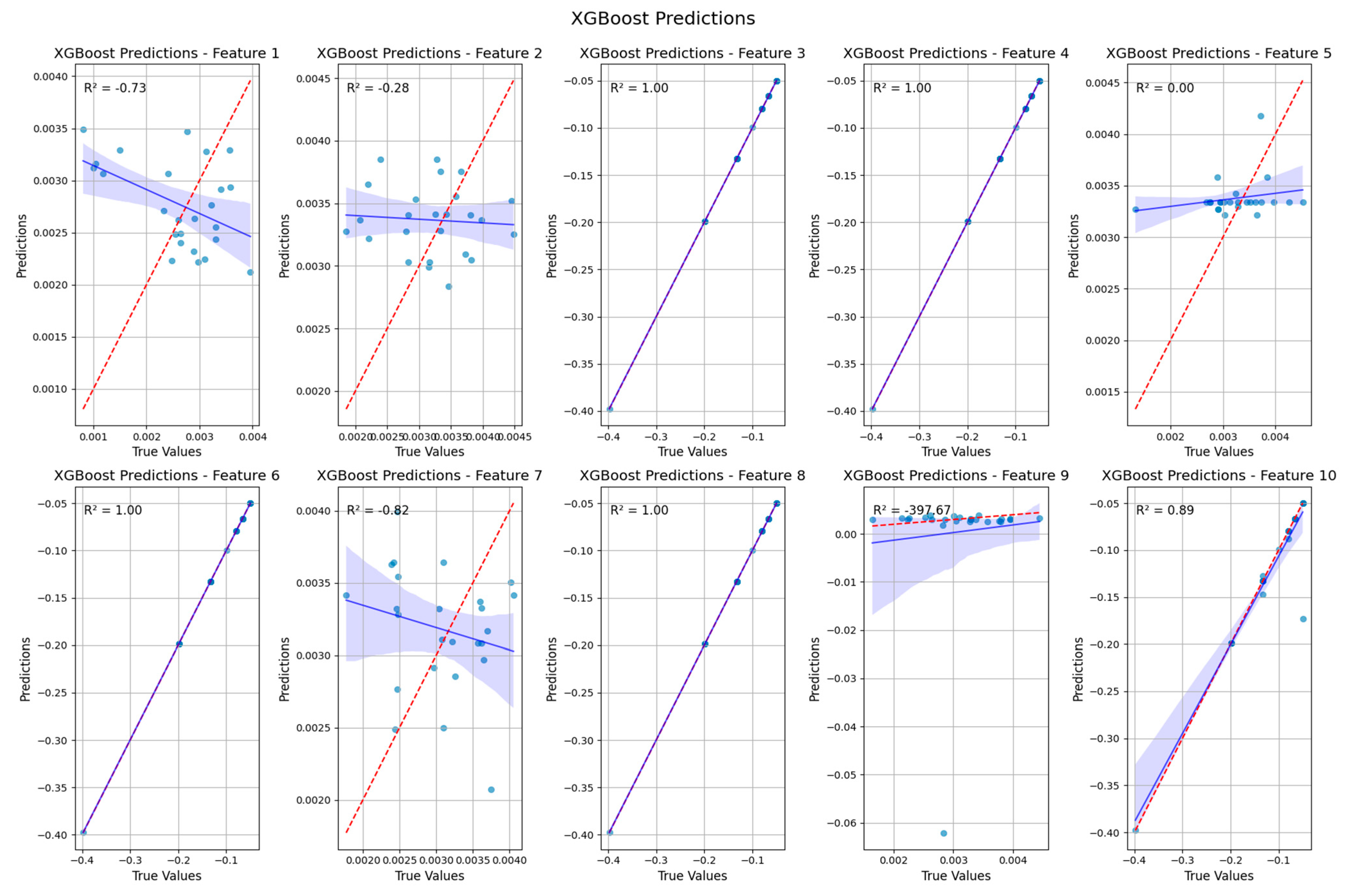
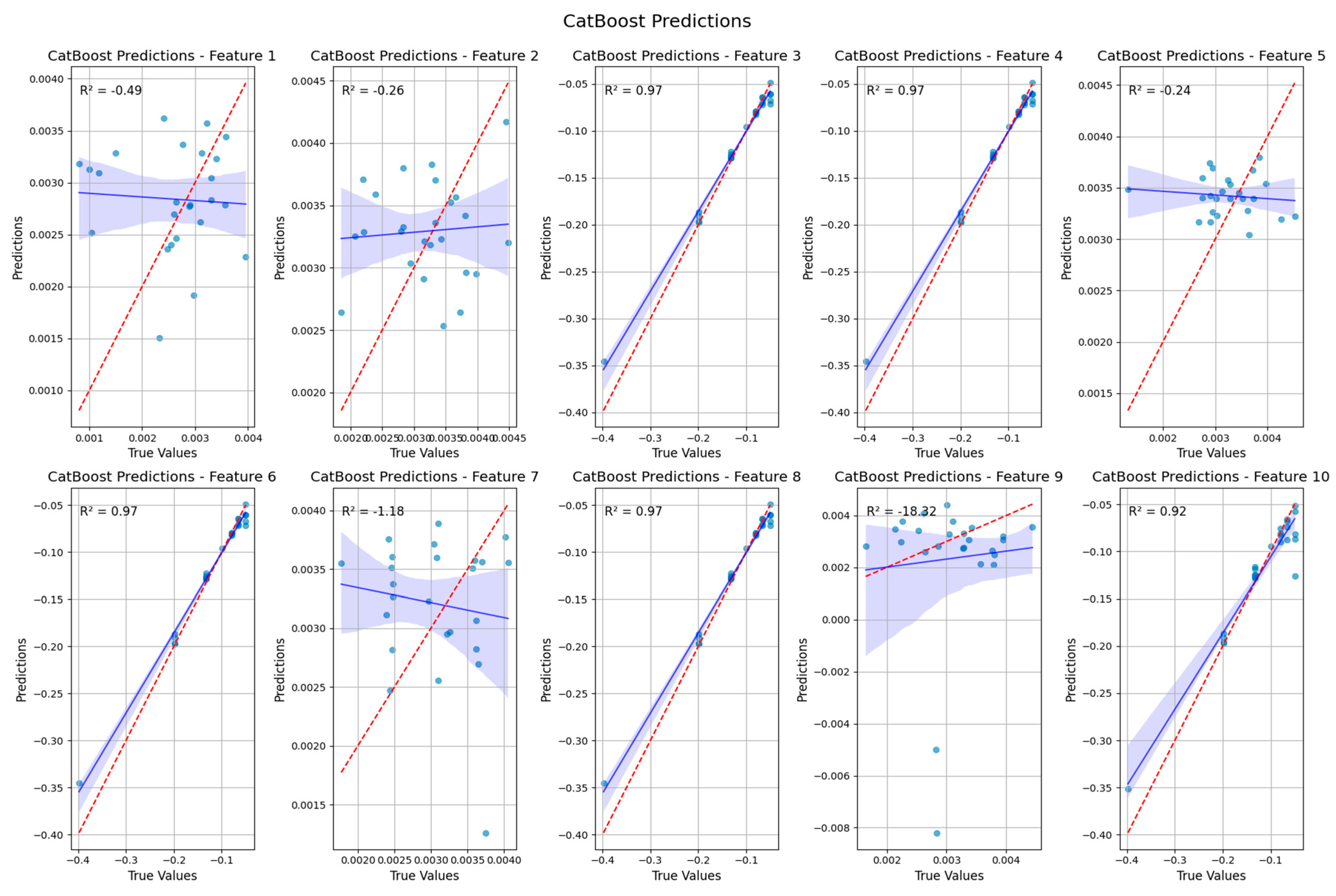
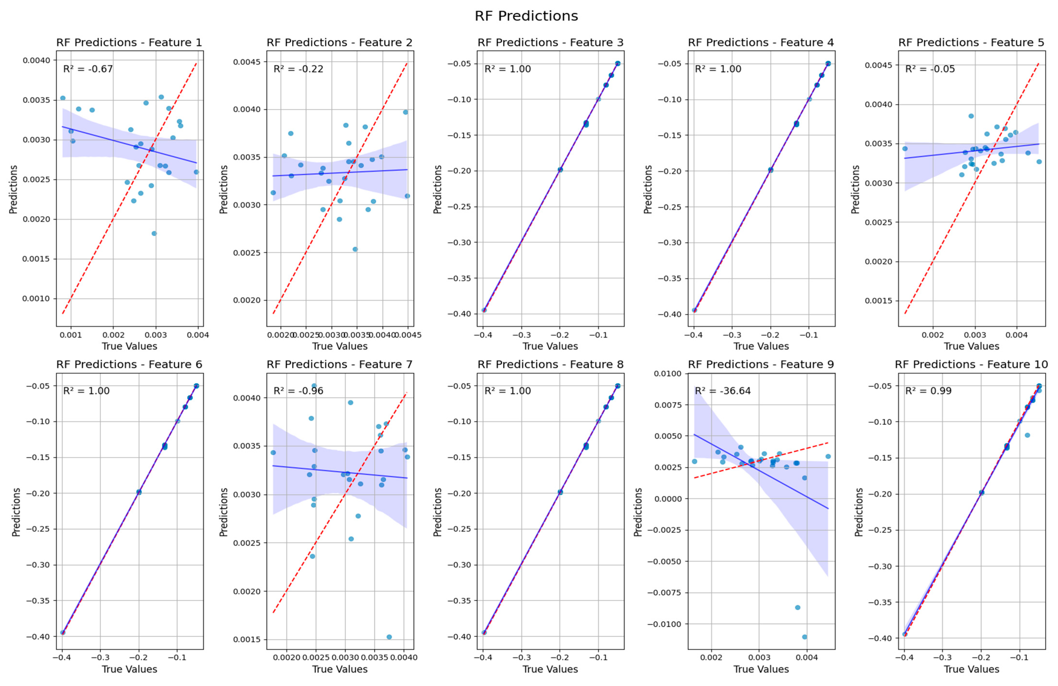
4.3. Machine Learning Results

Figure 27, Figure 28, Figure 29, Figure 30 and Figure 31 showcase the performance of the ML models in the prediction of carbon nanotube vibrations for displacement and frequency for five modes. Each scatter plot represents the bond between the predicted values and true values for a specific feature. The first five features represent the amplitude for five modes, and the next five represent the frequency in the same order.

In Figure 27 it can be observed that Features 3, 4, 6, and 8 show R² values of 1.00, indicating an almost perfect fit between the predicted and true values. With similar performance quotas, features 1, 7, and 10 show R² values between 0.42 and 0.89, suggesting a reasonable fit. Feature 2 has an R² of 0.28, indicating a moderate fit. Feature 5 has an R² of 0.00, suggesting a very poor fit. The model is unable to capture the relationship between the predicted and true values for this feature. Feature 9 has an extremely low R² value of −397.67, indicating a very poor fit and potential issues with the data or model for this feature.

The XGBoost model shows promising results for several features but struggles with others.

Features 3, 4, 6, and 8 show R² values of 0.97, indicating a very good fit between the predicted and true values, as shown in Figure 28. However, feature 10 has an R² of 0.92, suggesting a good fit. On the contrary, Features 1 and 5 have R² values between 0.24 and 0.49, indicating a moderate fit. Feature 2 has an R² of −0.26, suggesting a poor fit. The model is not capturing the relationship between predicted and true values well for this feature.

Features 7 and 9 have extremely low R² values, indicating a very poor fitness and potential issues with the data or model for these features. Overall, the CATBoost model shows promising results for several features but struggles with others.

Features 1, 4, 6, and 9: These features show an R² of 1.00, indicating a perfect fit as shown in Figure 29. This suggests the Random Forest models are performing exceptionally well for these features.

Other features: The R² values for the remaining features are negative or close to zero, suggesting a poor fit. The model is not performing well in predicting these features.

Overall, the Random Forest model appears to be effective in predicting certain vibrational modes of the carbon nanotube (features 1, 4, 6, and 9) but struggles with others.

Based on the R² values, the ANN model is performing extremely poorly for all features, as depicted by Figure 30. The R² values are extremely large and negative, indicating a very poor fit between the predicted and true values. This suggests that the ANN model is not able to capture the underlying patterns in the data and is making very poor predictions.

4.4. Comparison of Machine Learning Models for Carbon Nanotube Vibration Prediction

Having analyzed the performance of four models—Random Forest, XGBoost, CATBoost, and ANN—in predicting carbon nanotube vibrations based on provided visualizations provided in Figure 27, Figure 28, Figure 29 and Figure 30. The following performance summary is presented.

From Figure 31, XGBoost and CATBoost exhibit significantly lower MSE values than Random Forest and Neural Network, indicating superior performance in predicting the target variable as depicted by

Table 14. Machine learning models performance summary.

Model	Overall Performance	Strengths	Weaknesses
Random Forest	Moderate	Good performance on features 1, 4, 6, and 9	Poor performance on other features
XGBoost	Good	Excellent performance on features 3, 4, 6, and 8; good performance on others 1, 7, and 10	Fair performance on feature 2, poor performance on feature 5, very poor performance on feature 9
CATBoost	Good	Excellent performance on several features (3, 4, 6, and 8); good performance on feature 10	Fair performance on features 1 and 5, poor performance on feature 2, very poor performance on features 7 and 9
ANN	Very Poor	None	Poor performance on all features

. Random Forest demonstrates a moderate level of error, falling between the top-performing models and the Neural Network.

While Neural Network shows the highest MSE, suggesting that the model struggles to capture the underlying patterns in the data.

In addition to R² and MSE, we also evaluated model performance using the mean absolute error (MAE) and root mean square error (RMSE). MAE provides an average magnitude of error without penalizing large deviations disproportionately, while RMSE emphasizes larger errors due to its quadratic nature. These metrics allowed a more complete assessment of the regression models. XGBoost consistently achieved the lowest MAE and RMSE values across prediction tasks, confirming its robustness in modeling the nonlinear vibrational behavior of the system.

Although the machine learning models demonstrated good predictive power, some limitations were apparent, particularly in the representation of higher-mode complicated nonlinear interactions. Several reasons may be attributable to this. To begin with, the relatively small dataset size, although it covered a broad matrix of physical parameters, might have constrained the generalizability of the models in all situations. Second, feature correlations and variation among inputs, especially between mass coefficient, stability frequency, and magnetic flux, might have introduced latent biases to model learning. In addition, simulation noise and boundary condition assumptions can lead to small differences between training data and physical reality. Feature importance analysis showed that certain features had a dominating impact on the model predictions, which meant that under-represented features (e.g., branch angle interactions at high velocities) would need to be further refined for future datasets. Refinement of these aspects, e.g., data volume expansion, feature engineering, and noise reduction, will continue to enhance the usability and robustness of ML models for difficult nanoscale vibration problems.

5. Conclusions

This study presented a comprehensive approach to modeling and analyzing the nonlinear fluid-induced vibration of pronged single-walled carbon nanotubes (SWCNTs) subjected to thermal and magnetic fields. Through a combination of analytical modeling using the Euler–Bernoulli and Eringen nonlocal theories, numerical simulation via ANSYS, and predictive modeling with machine learning algorithms (XGBoost, CATBoost, Random Forest, and Neural Networks), we identified the critical parameters influencing system stability, including branching angle, magnetic flux density, flow velocity, and foundation stiffness.

The parametric analysis led to the following key findings:

• The angle at which the nanotube branches significantly affects its stability. A larger angle has been demonstrated to reduce stability.
• The dynamic behavior of the SWCNT is dampened by the existing magnetic field introduced to the environment.
• The nonlocal term has a major impact on flow velocity and frequency. Furthermore, raising the foundation parameters and shear moduli increases the fundamental frequency of the nanotube.
• The fluid–structure mass ratio becomes particularly important in post-bifurcation regions, where frequencies and velocities increase with rising temperatures.
• The difference between linear and nonlinear vibration frequencies becomes more pronounced as flow velocity and amplitude rise.
• Increasing axial pre-tension on the nanotube reduces its stability, especially as it deviates further from linear behavior.

In addition to magnetic effects, temperature also plays a critical role in influencing the vibrational characteristics of branched SWCNTs. As temperature increases, thermal expansion leads to a reduction in the effective stiffness of the nanotube material, resulting in lower natural frequencies and greater susceptibility to instability under fluid flow. This softening effect reduces the critical flow velocities at which bifurcation or flutter phenomena are observed.

The novel integration of machine learning algorithms with physics-based models provides rapid, accurate predictions and optimization strategies for enhancing system stability at the nanoscale. This integration offers a new pathway for designing nanostructures in energy harvesting, biomedical devices, and nanofluidic systems where real-time vibrational control is essential.

Future work may involve expanding the dataset through further simulations and experimental validation, exploring additional environmental conditions such as multi-physics couplings (piezoelectric effects, electro-thermal fields), and testing alternative machine learning architectures, including ensemble deep learning methods, to enhance predictive accuracy.

References

1. Chen, X.; Zhao, J.; She, G.-L.; Luo, J. Nonlinear free vibration analysis of functionally graded carbon nanotube reinforced fluid-conveying pipe in thermal environment. Steel Compos. Struct. 2022, 35, 641–652. [Google Scholar] [CrossRef]
2. Saifuddin, N.; Raziah, A.Z.; Junizah, A.R. Carbon Nanotubes: A Review on Structure and Their Interaction with Proteins. J. Chem. 2013, 2013, 676815. [Google Scholar] [CrossRef]
3. Rust, C.; Shapturenka, P.; Spari, M.; Jin, Q.; Li, H.; Bacher, A.; Guttmann, M.; Zheng, M.; Adel, T.; Hight Walker, A.R.; et al. The Impact of Carbon Nanotube Length and Diameter on their Global Alignment by Dead-End Filtration. Small 2023, 19, 2206774. [Google Scholar] [CrossRef]
4. Sakharova, N.A.; Pereira, G.A.F.; Antunes, J.M.; Fernandes, J.V. Mechanical Characterization of Multiwalled Carbon Nanotubes: Numerical Simulation Study. Materials 2020, 13, 4283. [Google Scholar] [CrossRef]
5. Xu, L.; Jiao, X.; Shi, C.; Wu, A.-P.; Hou, P.-X.; Liu, C.; Cheng, H.-M. Single-Walled Carbon Nanotube/Copper Core–Shell Fibers with a High Specific Electrical Conductivity. ACS Nano 2023, 17, 9245–9254. [Google Scholar] [CrossRef]
6. Iijima, S. Helical microtubules of graphitic carbon. Nature 1991, 354, 56–58. [Google Scholar] [CrossRef]
7. Cui, K.; Chuang, J.; Feo, L.; Chow, C.; Lau, D. Developments and Applications of Carbon Nanotube Reinforced Cement-Based Composites as Functional Building Materials. Front. Mater. 2022, 9, 861646. [Google Scholar] [CrossRef]
8. Yinusa, A.; Sobamowo, M.; Adelaja, A. Nonlinear vibration analysis of an embedded branched nanofluid-conveying carbon nanotube: Influence of downstream angle, temperature change and two-dimensional external magnetic fields. Nano Mater. Sci. 2020, 2, 323–332. [Google Scholar] [CrossRef]
9. Mahmure, A.; Tornabene, F.; Dimitri, R.; Kuruoglu, N. Free Vibration of Thin-Walled Composite Shell Structures Reinforced with Uniform and Linear Carbon Nanotubes: Effect of the Elastic Foundation and Nonlinearity. Nanomaterials 2021, 11, 2090. [Google Scholar] [CrossRef]
10. Huang, K.; Yao, J. Beam Theory of Thermal–Electro-Mechanical Coupling for Single-Wall Carbon Nanotubes. Nanomaterials 2021, 11, 923. [Google Scholar] [CrossRef]
11. Shaba, A.I.; Jiya, M.; Aiyesimi, Y.M.; Mohammed, A.A. Vibration of Single–Walled Carbon Nanotube (SWCNT) on a Winkler Foundation with Magnetic Field Effect. Sci. World J. 2021, 16, 402–406. [Google Scholar]
12. Yinusa, A.; Sobamowo, M. Mechanics of nonlinear internal flow-induced vibration and stability analysis of a pre-tensioned single-walled carbon nanotube using classical differential transform method with CAT and SAT after-treatment techniques. Forces Mech. 2022, 7, 100083. [Google Scholar] [CrossRef]
13. Yan, Y.; Li, J.; Ma, X.; Wang, W. Application and dynamical behaviour of CNTs as fluidic nanosensors based on the nonlocal strain gradient theory. Sens. Actuators A Phys. 2021, 330, 112836. [Google Scholar] [CrossRef]
14. Chen, Y.; Lyu, M.; Zhang, Z.; Yang, F.; Li, Y. Controlled Preparation of Single-Walled Carbon Nanotubes as Materials for Electronics. ACS Cent. Sci. 2022, 8, 1490–1505. [Google Scholar] [CrossRef] [PubMed]
15. Miyashiro, D.; Taira, H.; Hamano, R.; Reserva, R.L.; Umemura, K. Mechanical vibration of single-walled carbon nanotubes at different lengths and carbon nanobelts by modal analysis method. Compos. Part C Open Access 2020, 2, 100028. [Google Scholar] [CrossRef]
16. Dat, N.D.; Quan, T.Q.; Mahesh, V.; Duc, N.D. Analytical solutions for nonlinear magneto-electro-elastic vibration of the smart sandwich plate with carbon nanotube reinforced nanocomposite core in hygrothermal environment. Int. J. Mech. Sci. 2020, 186, 105906. [Google Scholar] [CrossRef]
17. De Rosa, M.A.; Lippiello, M.; Babilio, E.; Ceraldi, C. Nonlocal Vibration Analysis of a Nonuniform Carbon Nanotube with Elastic Constraints and an Attached Mass. Materials 2021, 14, 3445. [Google Scholar] [CrossRef]
18. Oveissi, S.; Eftekhari, S.A.; Toghraie, D. Longitudinal vibration and instabilities of carbon nanotubes conveying fluid considering size effects of nanoflow and nanostructure. Phys. E Low-Dimens. Syst. Nanostruct. 2016, 83, 164–173. [Google Scholar] [CrossRef]
19. Chang, X.; Hong, X.; Qu, C.; Li, Y. Stability and nonlinear vibration of carbon nanotubes-reinforced composite pipes conveying fluid. Ocean. Eng. 2023, 281, 114960. [Google Scholar] [CrossRef]
20. Sabahi, M.A.; Saidi, A.R.; Khodabakhsh, R. An analytical solution for nonlinear vibration of functionally graded porous micropipes conveying fluid in damping medium. Ocean. Eng. 2022, 245, 110482. [Google Scholar] [CrossRef]
21. Moborukoje, K.I.; Oladosu, S.; Kuku, R.; Sobamowo, G. Exploring the Significances of Surface Energy, Initial Stress and Nonlocality Effects on Vibration of Carbon Nanotubes Conveying Fluid Resting on Elastic Foundations in a Magneto-Thermal Environment. World Sci. News 2022, 179, 112–134. [Google Scholar]
22. Ghadirian, H.; Mohebpour, S.; Malekzadeh, P.; Daneshmand, F. Nonlinear free vibrations and stability analysis of FG-CNTRC pipes conveying fluid based on Timoshenko model. Compos. Struct. 2022, 292, 115637. [Google Scholar] [CrossRef]
23. Heidary, Z.; Ramezani, S.R.; Mojra, A. Exploring the benefits of functionally graded carbon nanotubes (FG-CNTs) as a platform for targeted drug delivery systems. Comput. Methods Programs Biomed. 2023, 238, 107603. [Google Scholar] [CrossRef] [PubMed]
24. Oveissi, S.; Ghassemi, A.; Salehi, M.; Eftekhari, S.A.; Ziaei-Rad, S. Hydro–Hygro–Thermo–Magneto–Electro elastic wave propagation of axially moving nano-cylindrical shells conveying various magnetic-nano-fluids resting on the electromagnetic-visco-Pasternak medium. Thin-Walled Struct. 2022, 173, 108926. [Google Scholar] [CrossRef]
25. Oveissi, S.; Salehi, M.; Ghassemi, A.; Ali Eftekhari, S.; Ziaei-Rad, S. Energy harvesting of nanofluid-conveying axially moving cylindrical composite nanoshells of integrated CNT and piezoelectric layers with magnetorheological elastomer core under external fluid vortex-induced vibration. J. Magn. Magn. Mater. 2023, 572, 170551. [Google Scholar] [CrossRef]
26. Yinusa, A.; Sobamowo, M.; Adelaja, A.; Ojolo, S.; Waheed, M.; Usman, M.; Siqueira, A.M.D.O.; Campos, J.C.C.; Ola-Gbadamosi, R. Numerical investigation on the thermal-nanofluidic flow induced transverse and longitudinal vibrations of single and multi-walled branched nanotubes resting on nonlinear elastic foundations in a magnetic environment. Partial Differ. Equ. Appl. Math. 2024, 9, 100602. [Google Scholar] [CrossRef]
27. Vivanco-Benavides, L.E.; Martínez-González, C.L.; Mercado-Zúñiga, C.; Torres-Torres, C. Machine learning and materials informatics approaches in the analysis of physical properties of carbon nanotubes: A review. Comput. Mater. Sci. 2021, 201, 110939. [Google Scholar] [CrossRef]
28. Pollayi, H.; Rao, P. Stealth Carbon Nano-tubes (S-CNTs): AI/ML Based Modelling of Nano-structured Composites for Attenuation and Shielding in Aircraft. In Proceedings of the International Symposium on Lightweight and Sustainable Polymeric Materials (LSPM23), Bangkok, Thailand, 17 February 2023; pp. 1–10. [Google Scholar] [CrossRef]
29. Čanađija, M. Deep learning framework for carbon nanotubes: Mechanical properties and modelling strategies. Carbon 2021, 184, 891–901. [Google Scholar] [CrossRef]
30. Yang, J.; Ni, Z.; Fan, Y.; Hang, Z.; Liu, H.; Feng, C. Machine learning aided uncertainty analysis on nonlinear vibration of cracked FG-GNPRC dielectric beam. Structures 2023, 58, 105456. [Google Scholar] [CrossRef]
31. Akbarzadeh, S.; Akbarzadeh, K.; Ramezanzadeh, M.; Naderi, R.; Mahdavian, M.; Olivier, M. Corrosion resistance enhancement of a sol-gel coating by incorporation of modified carbon nanotubes: Artificial neural network (ANN) modelling and experimental explorations. Prog. Org. Coat. 2022, 174, 107296. [Google Scholar] [CrossRef]
32. Khanam, P.N.; AlMaadeed, M.A.; AlMaadeed, S.; Kunhoth, S.; Ouederni, M.; Sun, D.; Hamilton, A.; Harkin Jones, E.; Mayoral, B. Optimization and Prediction of Mechanical and Thermal Properties of Graphene/LLDPE Nanocomposites by Using Artificial Neural Networks. Int. J. Polym. Sci. 2016, 2016, 5340252. [Google Scholar] [CrossRef]
33. Hajilounezhad, T.; Bao, R.; Palaniappan, K.; Bunyak, F.; Calyam, P.; Maschmann, M.R. Predicting carbon nanotube forest attributes and mechanical properties using simulated images and deep learning. NPJ Comput. Mater. 2021, 7, 134. [Google Scholar] [CrossRef]
34. Kekez, S.; Kubica, J. Application of Artificial Neural Networks for Prediction of Mechanical Properties of CNT/CNF Reinforced Concrete. Materials 2021, 14, 5637. [Google Scholar] [CrossRef] [PubMed]
35. Chen, T.; Guestrin, C. XGBoost: A Scalable Tree Boosting System. In Proceedings of the 22nd Acm Sigkdd International Conference on Knowledge Discovery and Data Mining, San Francisco, CA, USA, 13–17 August 2016. [Google Scholar] [CrossRef]
36. Sunday, G.J.; Oladosu, S.A.; Kuku, R.O.; Sobamowo, G.M.; Yinusa, A.A. Explorations of the combined effects of surface energy, initial stress and nonlocality on the dynamic behaviour of carbon nanotubes conveying fluid resting on elastic foundations in a thermo-magnetic environment. J. Nanosci. Technol. 2023, 1, 102. [Google Scholar]
37. Abubakar, E.H.; Sobamowo, M.G.; Sadiq, M.O.; Yinusa, A.A. Vibration of Single-walled Carbon Nanotubes Resting on Elastic Medium with Magnetic and Thermal Effects under the Influence of Electrostatic Force. World Sci. News 2024, 188, 93–118. [Google Scholar]
38. Selim, M.M.; Musa, A. Nonlinear Vibration of a Pre-Stressed Water-Filled Single-Walled Carbon Nanotube Using Shell Model. Nanomaterials 2020, 10, 974. [Google Scholar] [CrossRef]
39. Strozzi, M.; Elishakoff, I.E.; Bochicchio, M.; Cocconcelli, M.; Rubini, R.; Radi, E. A Comparison of Shell Theories for Vibration Analysis of Single-Walled Carbon Nanotubes Based on an Anisotropic Elastic Shell Model. Nanomaterials 2023, 13, 1390. [Google Scholar] [CrossRef]
40. Olaleye, T.I.; Oladosu, S.A.; Kuku, R.O.; Sobamowo, G.M. Variation iteration method to the investigations of surface energy, initial stress and nonlocality on vibration of carbon nanotubes conveying fluid resting on elastic foundations in a thermo-magnetic environment. J. Mater. Environ. Sci. 2023, 14, 520–538. [Google Scholar]
41. Brociek, R.; Pleszczyński, M. Differential Transform Method and Neural Network for Solving Variational Calculus Problems. Mathematics 2023, 12, 2182. [Google Scholar] [CrossRef]
Figure 1. Architecture of the machine learning models used in this study: (a) Random Forest; (b) XGBoost; (c) CATBoost; and (d) Artificial Neural Network. These models were selected to explore a range of regression methods for predicting vibrational and frequency responses under varying physical parameters.
Vibration 08 00035 g001
Figure 2. Nanofluid flows in branched nanotube.
Vibration 08 00035 g002
Figure 3. A simple supported branched SWCNT resting on an elastic foundation.
Vibration 08 00035 g003
Figure 4. Model building flow chart.
Vibration 08 00035 g004
Figure 5. Modal number’s impacts on the nanotube’s mode shapes for pinned-pinned supports.
Vibration 08 00035 g005
Figure 6. Branch angle impact on linear stability and nonlinear stability: (a) linear; (b) nonlinear.
Vibration 08 00035 g006
Figure 7. Branch angle impact on linear stability and nonlinear stability: (a) linear for post-bifurcation; (b) nonlinear for post-bifurcation; (c) linear pre- and post-bifurcation; (d) nonlinear pre- and post-bifurcation.
Vibration 08 00035 g007
Figure 8. Winkler’s foundations effects on stability of SWCNT.
Vibration 08 00035 g008
Figure 9. Vibrational dynamic responses of the SWCNT.
Vibration 08 00035 g009
Figure 10. The linear response at different modes (a) Linear response at mode 1 for B = 100; (b) Linear response at mode 1 for B = 120; (c) Linear response at mode 2 for B = 50; (d) Nonlinear response at mode 1 for B = 50.
Vibration 08 00035 g010
Figure 11. Values distribution for MFD and MFI for I-shaped nanotube: (a) magnetic flux density I-shaped; (b) vector representation of magnetic field intensity I-shaped.
Vibration 08 00035 g011
Figure 12. Values distribution MFI for Y-shaped nanotube with branch angle of 15°: (a) MFI of nanotube; (b) MFI vector representation of nanotube.
Vibration 08 00035 g012
Figure 13. Values distribution MFI for Y-shaped nanotube with branch angle of 30°: (a) MFI of nanotube; (b) MFI vector representation of nanotube.
Vibration 08 00035 g013
Figure 14. Values distribution MFI for Y-shaped nanotube with branch angle of 45°: (a) MFI of nanotube; (b) MFI vector representation of nanotube.
Vibration 08 00035 g014
Figure 15. Values distribution MFI for Y-shaped nanotube with branch angle of 60°: (a) MFI of nanotube; (b) MFI vector representation of nanotube.
Vibration 08 00035 g015
Figure 16. Values distribution MFI for Y-shaped nanotube with branch angle of 75°: (a) MFI of nanotube; (b) MFI vector representation of nanotube.
Vibration 08 00035 g016
Figure 17. Values distribution MFI for T-shaped nanotube with branch angle of 90°: (a) MFI of nanotube; (b) MFI vector representation of nanotube.
Vibration 08 00035 g017
Figure 18. Deformation by modes for I-shaped CNT with no periphery support.
Vibration 08 00035 g018
Figure 19. Deformation by modes for I-shaped CNT with elastic support.
Vibration 08 00035 g019
Figure 20. Deformation by modes for Y-shaped CNT (15°).
Vibration 08 00035 g020
Figure 21. Deformation by modes for Y-shaped CNT (30°).
Vibration 08 00035 g021
Figure 22. Deformation by modes for Y-shaped CNT (45°).
Vibration 08 00035 g022
Figure 23. Deformation by modes for Y-shaped CNT (60°).
Vibration 08 00035 g023
Figure 24. Deformation by modes for Y-shaped CNT (75°).
Vibration 08 00035 g024
Figure 25. Deformation by modes for T-shaped CNT.
Vibration 08 00035 g025
Figure 26. Values distribution of nanotubes for transient analysis: (a) transient structural I-shaped; (b) equivalent stress I-shaped; (c) equivalent stress Y-shaped; (d) equivalent stress T-shaped.
Vibration 08 00035 g026aVibration 08 00035 g026b
Figure 27. XGBoost performance evaluation.
Vibration 08 00035 g027
Figure 28. CATBoost performance evaluation.
Vibration 08 00035 g028
Figure 29. Random Forest performance evaluation.
Vibration 08 00035 g029
Figure 30. ANN performance evaluation.
Vibration 08 00035 g030
Figure 31. Comparing models performance evaluation.
Vibration 08 00035 g031