Vibration Signal-Based Fault Diagnosis of Rotary Machinery Through Convolutional Neural Network and Transfer Learning Method

Abstract

Artificial Intelligence (AI) is revolutionizing proactive repair systems by enabling real-time identification of bearing faults in industrial machinery. However, traditional fault detection methods often struggle in dynamic environments due to their dependence on specific training conditions. To address this limitation, a transfer learning (TL)-based methodology has been developed for bearing fault detection, so that the model trained under some specific training conditions can perform accurately under significantly different real-time working conditions, thereby significantly improving diagnostic efficiency while reducing training time. Initially, a deep learning approach utilizing convolutional neural networks (CNNs) has been employed to diagnose faults based on vibration data. After achieving high classification performance at source domain conditions, the performance of the model is re-evaluated by applying it to the Case Western Reserve University (CWRU) dataset as the target domain through the TL method. short-time Fourier transform is employed for signal preprocessing, enhancing feature extraction and model performance. The proposed methodology has been validated across various CWRU dataset configurations under different operating conditions and environments. The proposed approach achieved a 99.7% classification accuracy in the target domain, demonstrating effective adaptability and robustness under domain shifts. The results demonstrate how TL-enhanced CNNs can be used as a scalable and efficient way to diagnose bearing faults in industrial environments.

1. Introduction

Advanced electromechanical equipment forms the backbone of modern industrial operations, spanning manufacturing and infrastructure. For sustained productivity and to minimize environmental impact, ensuring the durability and reliable performance of the equipment is paramount [1,2]. Adopting preventative diagnostic strategies is vital to avoid costly equipment failures and enable timely maintenance. Bearing is one of the most crucial parts of rotary equipment, and when they fail, not only do they lower the productivity of the industrial production process and result in financial losses, but they also endanger the safety of human production. Machine fault diagnosis (FD) is the process of maintaining machinery by evaluating the subsystems’ current state of health [3,4]. Choosing the right sensors is essential for accurate monitoring, as each is designed to capture distinct aspects of machine performance.

Vibration analysis, a form of mechanical quantity sensing, is widely used for its effectiveness in early fault detection [5,6]. Other commonly used sensors monitor displacement, torque, angular velocity/position, current, and voltage. Additional data sources, such as temperature (internal and external), sound, and chemical composition, can provide valuable insights depending on the fault type being analyzed [7]. Diagnostic methods are evolving, with image-based techniques employing cameras to visually assess machine health. Furthermore, signal-to-image conversion is being developed, enabling the application of image processing for FD. The ability to detect subtle changes in operational conditions makes vibration analysis a popular method for identifying faults in rotary machinery. However, traditional methods may face limitations in intricate scenarios, particularly when analyzing non-stationary faults [8]. The advancement of smart manufacturing has significantly accelerated data collection and introduced opportunities and challenges for the industry. As a result, data-driven FD has gained considerable research attention in recent years [9]. This approach is particularly beneficial for complex systems where defining explicit models or signal patterns is challenging. However, it relies on large volumes of historical data to uncover meaningful insights about system behavior. Data can now be gathered considerably more quickly thanks to the growth of smart manufacturing, which presents the sector with new challenges and prospects. As a result, machine learning (ML) techniques are frequently used in data-driven fault diagnostics [10,11]. These are reliant on manually chosen characteristics, so if these features are insufficient for the diagnostic task, fault detection performance may decrease significantly. Furthermore, features that perform well for making predictions in one scenario might not perform well in another because handcrafted features are task-specific for different categorization tasks. Creating a single set of parameters capable of consistently producing precise predictions across all conditions is a complex task. Deep learning (DL) techniques offer efficient ways to get around these restrictions, in part because of their strong feature learning capabilities [12]. Multiple hidden layers in deep architectures offer the capacity to directly extract hierarchical features from the raw input. These architectures can automatically choose discriminative representations through model training that are helpful for creating precise predictions in later classification stages in accordance with the training data.

The effectiveness of traditional ML techniques stems from the general assumption that the training (source) and testing (target) data originate from the same distribution. Therefore, the effectiveness of these strategies would decrease if the distributions were different. In many applications in engineering, this assumption is incorrect. The issue also affects deep learning methodologies. To address this issue, an intelligent vibration signals-based FD approach has been proposed using a convolutional neural network (CNN) with transfer learning (TL) under varying operating scenarios to detect bearing faults. The findings across the target dataset demonstrate the capability of the proposed method in accurately identifying the bearing fault, thereby making a valuable addition to the bearing FD technologies.

The article’s remaining content is arranged as follows: The theory pertaining to data-driven fault diagnostic and TL is covered in Section 2, whereas the approach used for bearing fault diagnostics is presented in Section 3. The results obtained for different datasets to validate the proposed methodology are discussed in Section 4. Section 5 draws the article’s conclusions and explains future prospects.

2. Related Work

This section covers the existing research on data-driven FD and transfer learning.

2.1. Data-Driven Fault Diagnostic Methods

Modern FD increasingly favors data-centric strategies, which excel at interpreting intricate equipment behavior without relying on explicit mathematical models. These methods utilize sensor-acquired information, such as vibration, acoustic, and thermal signals, to identify, classify, and predict faults in rotating machinery. ML and DL techniques, such as support vector machines (SVMs), artificial neural networks (ANNs), and CNN, are instrumental in extracting meaningful features from raw data, which improves the accuracy of fault detection. Furthermore, sophisticated signal processing methods like wavelet transform (WT) and Hilbert transform improve feature extraction, which makes data-driven approaches very successful for predictive maintenance and real-time monitoring. Yin and Hou [13] reviewed advancements in SVM-based FD and process monitoring, emphasizing its effectiveness in handling complex industrial systems where direct observation is challenging. Their study highlights SVM’s superior generalization performance, particularly in scenarios with limited fault data, making it a valuable tool for fault detection and monitoring. Goyal et al. [14] introduced a non-contact FD system for bearings based on SVM. They developed a cost-effective vibration sensor and employed discrete wavelet transform for signal denoising. Feature selection was performed using the Mahalanobis distance criterion, followed by SVM classification. Their findings indicate that the non-contact sensor achieves performance comparable to conventional accelerometers in detecting bearing faults. You et al. [15] proposed an FD model for rotating machinery by integrating vibration severity analysis with wavelet-based feature extraction (VWC) and modified shuffled frog-leaping algorithm (MSFLA) SVM. Their study highlights the effectiveness of MSFLA in avoiding local optima and improving fault classification accuracy compared to traditional neural networks and SVM-based approaches. Goyal et al. [16] designed a non-contact vibration measurement system for fault detection in bearings using machine learning techniques. Their study compared ANN and SVM for classification and demonstrated that the proposed system provides high classification accuracy while eliminating the need for direct sensor contact. Morales et al. [17] proposed an FD method for three-phase induction motors using feature fusion from stator current and vibration signals, with SVM as the classification algorithm. Goyal et al. [5] developed a non-contact FD system for bearings using vibration response analysis. They utilized the Hilbert transform for denoising, applied principal component analysis (PCA) for dimensional reduction, and employed k-nearest neighbor (kNN) and weighted kNN classifiers for fault detection. Their results demonstrate that non-contact vibration sensors can provide reliable fault detection with minimal installation constraints. A two-stage FD method was presented by Zhang et al. [18] that combines SVM for fault identification with optimized support vector data description (SVDD) for fault detection. The grasshopper optimization algorithm was employed for parameter optimization, while refined composite multi-scale fuzzy entropy was utilized for feature extraction.

Beginning in the 1990s, learning methodologies were largely shaped by ML techniques, but a breakthrough occurred in 2010 with the emergence of deep neural networks (DNN), commonly known as deep learning (DL). DL and ML contribute to the broader field of artificial intelligence, which enables machines to simulate human intelligence without explicit programming [19]. Zhang et al. [20] explored the role of DL in prognostics, categorizing fault detection, FD, and remaining useful life (RUL) prediction into binary classification, multi-class classification, and continuous regression. Chen et al. [21] developed a low-dimensional feature set for deep belief networks (DBN) using intrinsic mode functions extracted from vibration data via integrated empirical mode decomposition (EEMD). Pan et al. [22] utilized discrete WT to process vibration signals and found that energy indices are highly sensitive to bearing faults when used with DBN for diagnosis. Yang et al. [23] reviewed an autoencoder (AE)-based FD, discussing optimization techniques, challenges, and future directions. Koutsoupakis et al. [12] employed CNN for bearing damage detection through simulations and experiments, optimizing SVDD using grasshopper optimization. Chen et al. [24] combined CNN for feature extraction and LSTM for down sampling and fault identification, significantly reducing model complexity. Liu et al. [25] introduced non-linear predictive denoising AEs based on gated recurrent units to enhance anomaly detection and fault classification while effectively mitigating noise interference. To overcome CNN and RNN limitations, Wei et al. [26] proposed WSAFormer-DFFN, a model integrating a self-attention mechanism with CNN for intelligent gearbox and bearing FD.

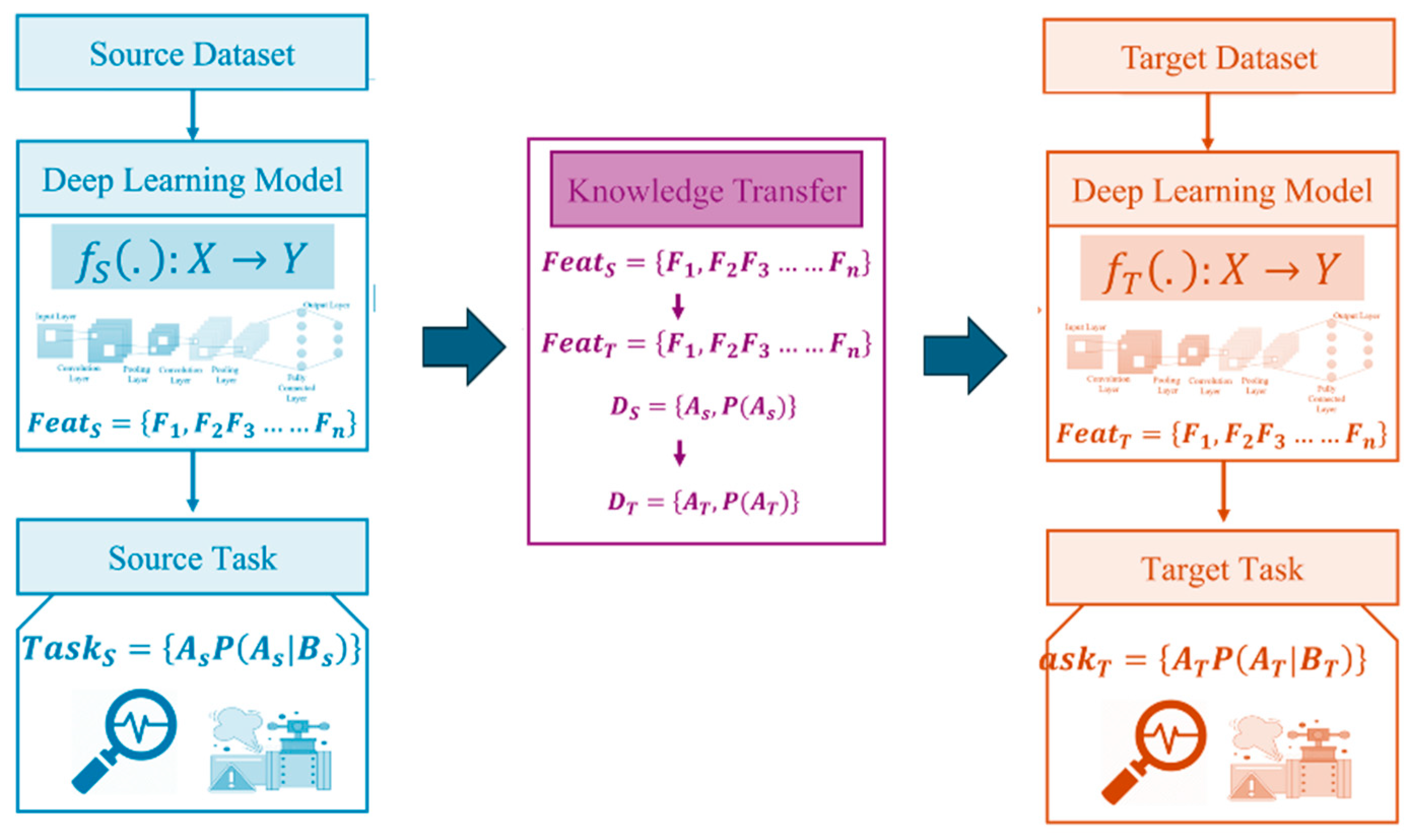
2.2. Transfer Learning

While deep learning techniques can significantly enhance fault classification accuracy, their effectiveness depends on two critical factors: first, the datasets used for training as well as testing should have similar distribution; second, a substantial, dataset is required to achieve high accuracy. However, in real-world industrial settings, variations in data distribution are inevitable due to factors such as environmental changes, installation differences, and varying operating conditions. This variation in the source (training) domain versus the target (testing) domain is called domain shift. To address this challenge, various TL methodologies have been applied for intelligent FD in rotating machinery. Zheng et al. [27] summarized current cross-domain FD research, examining the research impetus and cross-domain techniques. In these scenarios, TL is used to apply knowledge of the source domain to improve classification related to the target domain consisting of different data distributions. CNN-based domain-adaptive motor FD method was introduced by Xiao et al. [28] for extracting multi-layered features from unprocessed acceleration signals. To reduce distribution disparities between the source and target datasets, they integrated maximum mean discrepancy into the training process. Similarly, Guo et al. [29] developed a deep convolution TL network. It is made up of two modules: one for domain adaptation and the other for condition recognition, thereby ensuring the domain-invariant feature extraction possible. Their algorithm effectively identifies unlabeled target domain data after being trained on labeled source domain data. To address issues related to uneven domain data, Dong et al. [30] presented a refined TL strategy, utilizing CNNs and correlation alignment for cross-domain FD of bearings and gearboxes. DL-based feature correlation matching model was proposed by Wang et al. [31] to reduce domain differences and accurately pinpoint bearing faults. Shao and Kim [32] introduced an adaptive multi-scale CNN along with an attention mechanism to manage domain shifts and feature variations in the gearbox and bearing FD. Sun et al. [10] devised a new TL framework for rotating machinery fault identification, combining a dynamic multi-scale representation and a multi-path merging model. For scenarios with limited data samples, Zhang et al. [33] suggested the method of federated learning (FL) for the classification of bearing and gearbox faults, while ensuring the privacy of data. Xu et al. [34] introduced an open-set cross-domain FD approach, integrating FL with adversarial domain adaptation, to detect previously unseen gearbox faults.

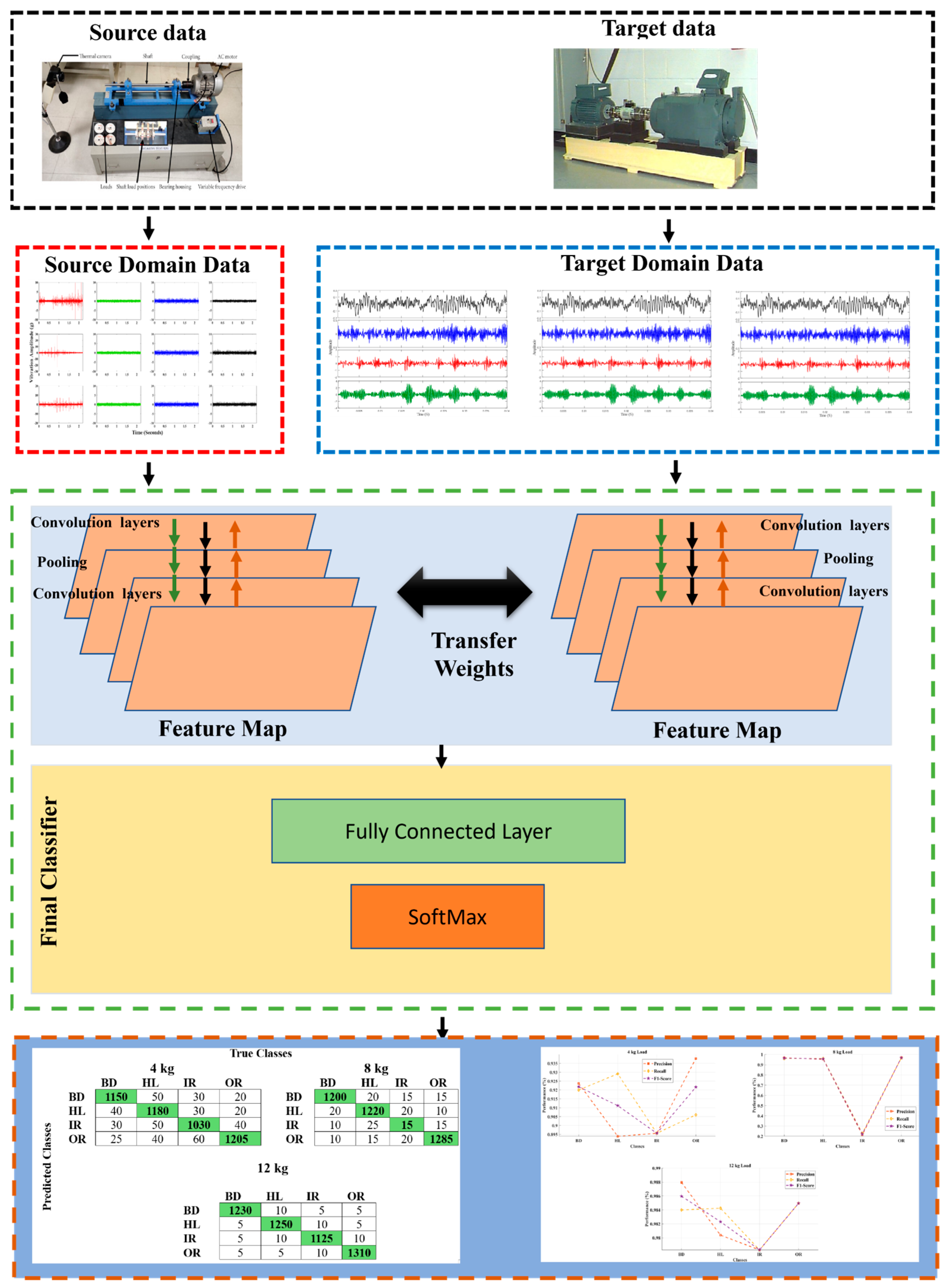
3. Experimental Methodology

The efficacy of transfer learning is largely contingent on how closely the source and target tasks resemble each other. The proposed methodology for effectively diagnosing bearing faults across various industrial contexts utilizes a CNN that takes preprocessed vibration sensor data as input. By integrating TL through a previously trained CNN model, the framework achieves a substantial improvement in diagnostic accuracy. Figure 1 presents the TL-driven framework applied for bearing FD. The procedural steps are detailed as follows:

(a)

The analysis and preprocessing using STFT of an accelerometer sensor dataset obtained from different industrial settings.

(b)

The dataset is categorized into source and target domains to facilitate the training and evaluation of the proposed model.

(c)

DL model using a CNN is developed using source domain data and its performance is evaluated.

(d)

The framework and hyperparameters of the previously trained model based on the source domain dataset have been designed and then fine-tuned to transfer to the targeted domain datasets.

(e)

The performance of the proposed TL-based framework has been assessed using the CRWU dataset.

There are two primary domains: the source domain, incorporating vibration signals captured under particular load and speed conditions, and the target domain, which is CWRU data acquired under different operating conditions. A CNN model is first trained on the data from the source domain, acquiring generalized fault features. Next, the model is fine-tuned with the classification layers being adapted with the data from the target domain to improve under domain shift conditions. The final prediction is made with the help of a Softmax layer, which calculates the probability distribution over the specified fault classes. The Final Classifier block is for the decision-making process, delivering the predicted fault class for every input example.

3.1. Conceptual Framework

Transfer learning (TL) facilitates the learning of a new task by drawing on knowledge gained from a previously learned task. The primary purpose of TL is to apply this gained information and expertise to a new, yet related, task. Its effectiveness lies in reducing the training time and complexity required to perform the target task. In this process, the task can be represented as $T=\left[A_T{P}_T\left(A_T|B_T\right)\right]$, where $A_T$ denotes the task and $P_T\left(A_T|B_T\right)$ represents the conditional probability distribution in the target domain. The process involves utilizing a feature space from the source domain, denoted as ${Feat}_S=[F_1{F}_2{F}_3\dots F_n]$, along with the conditional probability-distribution ${P\left(A_S\right|B}_S$) from the source domain to facilitate the learning of the target task.

This study examines four bearing conditions across both the source and target datasets. The process of knowledge transfer for bearing fault detection is described as follows: Let ${LB}_S$ represent a set of vibration data obtained from the source domain, and ${LB}_T$ represents a set of bearing fault data obtained from the target domain. The objective is to classify bearing faults in the target domain by transferring the knowledge (i.e., learned attributes) from the source domain. In this study, a model-based TL approach using CNNs has been employed. The source domain consisted of faulty data acquired under various operating situations, while the target domain consisted of data from different environmental settings, as illustrated in Figure 2.

The feature-based TL approach can be mathematically formulated as follows:

$$F_s\left(x\right)=W_s^{T}x+b_s$$

$$F_t\left(x\right)=W_t^{T}x+b_t$$

where $F_s{\mathrm{a}\mathrm{n}\mathrm{d}F}_t$ are the source and target domain feature extractors, respectively. $W_s$ and $W_t$ are the corresponding weight matrices, and $b_s$ and $b_t$ are the bias terms. The goal is to use the features learned in the source domain $F_s\left(x\right)$ to enhance the target domain model’s performance $F_t\left(x\right)$. The model-based TL approach can be expressed as follows:

$$F_s\left(x\right)={g(f}_s\left(x\right))$$

$$F_t\left(x\right)={h(f}_s\left(x\right),x)$$

Here, $F_t$ is the target domain model, $F_s$ is the source domain model, $g$ and $h$ are the adaptation functions, and $f_s\left(x\right)$ is the base feature extractor from the source domain. The aim is to adapt the source domain model $F_s\left(x\right)$ for effective use in the target domain through transformation functions $g$ and $h$. These mathematical formulations capture the key ideas behind feature-driven and model-driven TL, each of which is commonly applied in the bearing FD.

3.2. TL and Fine-Tuning Strategy

TL offers an efficient solution by utilizing a pre-trained deep (CNN) trained on a different dataset. CNNs, as previously noted, are capable of learning structured data representations from pictures, which makes it possible to efficiently transfer the information embedded in a pre-trained model’s weights to new tasks. Lower layers in the CNN specialize in identifying simple features like edges and curves, which tend to be useful across different image classification scenarios. Meanwhile, deeper layers focus on extracting complex and specialized features tailored to the specific task. This suggests that high-level representations usually require relearning from the destination dataset, but lower-level properties may frequently be transferred directly. The adaptation of the upper hidden layer weights to align with new data is known as fine-tuning. The required amount of fine-tuning depends on the degree of resemblance between the source and target datasets. For closely related datasets, fine-tuning can sometimes be restricted to the fully connected layers. However, if the datasets differ greatly, several convolutional blocks may need to be updated. A thorough layer-by-layer breakdown of the multi-input CNN architecture is given in

Table 1. Proposed multi-input CNN-based model architecture design for bearing FD.

Layer	Type	Activations	Learnable Property
imageinput_1	Image Input	100(S) × 100(s) × 3(C) × 1(B)	-
conv_1	2-D Convolution	100(S) × 100(s) × 3(C) × 1(B)	Weights: 3 × 3 × 3 × … Bias: 1 × 1 × 8…
relu_1	ReLU	100(S) × 100(s) × 3(C) × 1(B)	-
norm_1	Cross-channel Normalization	100(S) × 100(s) × 3(C) × 1(B)	-
maxpool_1	2-D Max Pooling	49(S) × 49(s) × 8(C) × 1(B)	-
conv2_1	2-D Grouped Convolution	49(S) × 49(s) × 8(C) × 1(B)	Weights: 3 × 3 × 4 × … Bias: 1 × 1 × 16…
relu_2	ReLU	49(S) × 49(s) × 8(C) × 1(B)
norm_2	Cross-channel Normalization	49(S) × 49(s) × 8(C) × 1(B)	-
maxpool_2	2-D Max Pooling	24(S) × 24(s) × 32(C) × 1(B)
conv_3	2-D Convolution	24(S) × 24(s) × 16(C) × 1(B)	Weights: 3 × 3 × 32 × ... Bias: 1 × 1 × 16…
relu_3	ReLU	24(S) × 24(s) × 16(C) × 1(B)
conv2_2	2-D Grouped Convolution	24(S) × 24(s) × 32(C) × 1(B)	Weights: 3 × 3 × 8 × … Bias: 1 × 1 × 16…
relu_6	ReLU	24(S) × 24(s) × 32(C) × 1(B)
conv2_3	2-D Grouped Convolution	24(S) × 24(s) × 16(C) × 1(B)	Weights: 3 × 3 × 16 × ... Bias: 1 × 1 × 8…
relu_7	ReLU	24(S) × 24(s) × 16(C) × 1(B)	-
maxpool_3	2-D Grouped Convolution	24(S) × 24(s) × 16(C) × 1(B)	-
conv_4	2-D Convolution	12(S) × 12(s) × 32(C) × 1(B)	Weights: 3 × 3 × 16 × ... Bias: 1 × 1 × 32…
relu_4	ReLU	12(S) × 12(s) × 32(C) × 1(B)	-
drop_1	Dropout (50%)	12(S) × 12(s) × 32(C) × 1(B)	-
fc_1	Fully Connected	4096(C) × 1(B)	Weights: 4096 × 46 × ... Bias: 4096 × 1…
relu_5	ReLU	4096(C) × 1(B)	-
drop_2	Dropout (50%)	4096(C) × 1(B)
fc_2_1	Fully Connected	20(C) × 1(B)	Weights: 20 × 4096 Bias: 20 × 1
Output	Fully Connected	20(C) × 1(B)	Weights: 20 × 40 Bias: 20 × 1

S—height, s—width, C—number of channels, B—batch size, weights represent the kernel size and depth, and bias indicates the number of bias terms corresponding to the output channels.

. The fine-tuning of the pre-trained CNN model was performed using an initial learning rate of 0.001, with a maximum of 20 epochs to ensure convergence while preventing overfitting. A mini-batch size of 32 was used to balance computational efficiency and gradient stability. To monitor performance during training, a validation frequency of 8 iterations was maintained, facilitating early detection of overfitting and ensuring robust model generalization.

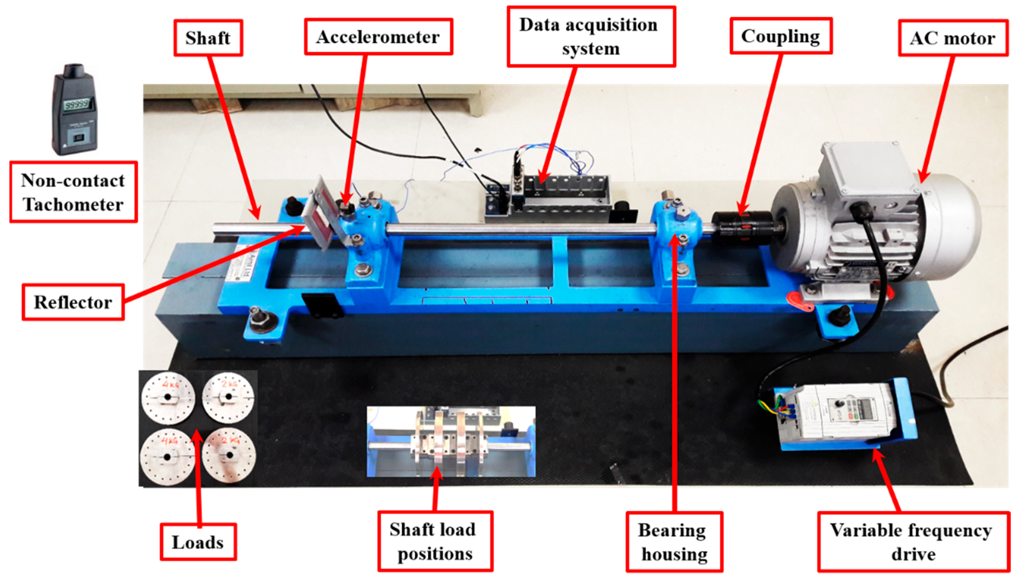
4. Experimental Setup and Data Processing

Figure 3 shows the testing apparatus used in this work to collect vibration data for training and testing bearing FD models. This experimental setup provides conditions akin to real-world operation for a rotor-bearing system. In this system, the rotor is composed of a driven shaft held by bearings at two support points, with the rotational speed being measured at the rotor coupling. Three rotor speeds (1000, 1200, and 1400 rpm) and loading conditions (0 kg, 4 kg, and 8 kg) were part of the test conditions. An electric discharge machine (EDM) was used to introduce various bearing fault types, including ball defect (BD), outer race defect (ORD), and inner race defect (IRD).

Vibration signals under various bearing conditions were captured using an accelerometer. Thirty thousand samples were gathered for the different test cases, using a sampling rate of 12.8 kHz. To determine the mean values of the statistical parameters, each experiment was conducted five times. Additionally, a healthy (H) bearing’s vibration signal provided the baseline for assessing fault conditions. This material offers a thorough rundown of the experimental process that produced the vibration-related data needed to diagnose bearing faults. The modular design of the experimental setup allows for easy removal and replacement of bearings. Figure 4 depicts both the healthy and defective bearing conditions used for vibration data collection. The specifications of the bearing considered in the current work are listed in

Table 2. Technical specifications of the bearing.

Characteristics	Specification	Characteristics	Specification
Type	SKF 1205 EKTN9	Contact angle (°)	10.583
Number of rollers per row	13	Pitch diameter (mm)	38.376
Number of rows	2	Ball diameter (mm)	7.5

.

The raw signals are illustrated in Figure 5, in which the red color represents ball defects, green corresponds to a healthy condition, blue indicates IRD, and black denotes ORD.

Under real-life conditions, the unprocessed vibration data are extremely complex, with critical information largely obscured by noise. In the case of good bearing condition (H), vibration variations are subtle and generally go unnoticed. However, across all bearing states, the maximum vibration amplitude has been consistently observed at maximum load and speed. As the load on the system increases, the vibration response intensifies, causing the time–domain signal to exhibit more pronounced spikes—characterized by sharp, short pulses—indicating the presence of a defect. For bearing with ORD, signal waveforms exhibit some distortion, although no obvious fault symptoms are visible. In contrast, bearing with IRD exhibits a significant increase in waveform spikes compared to healthy and OR conditions, indicating the fault’s presence. Interestingly, as the load increases, the signal becomes less spiky, possibly due to shaft wobbling effects, because there is a direct coupling between the IR and the transmission shaft. Further, among all bearing states, the BD condition exhibits the most noticeable differences in both amplitude and spike count, which is attributed to the impact forces generated when the ball defect comes to another bearing element, resulting in a strong impulsive response. However, despite these observations, it is difficult to differentiate defect types based solely on time–domain vibration signals. Therefore, further analysis using frequency domain techniques is paramount to precisely detect and diagnose bearing faults.

Data Preprocessing

In real-time applications, signals are typically non-stationary (frequency components change over time) and the Short-time Fourier Transform (STFT) is considered as an essential tool for analyzing such signals. In this work, STFT is employed by dividing the vibration signal into smaller, overlapping segments to enable localized analysis. The FT is then applied to each segment, using a window function to diminish spectral leakage. The time–frequency resolution of STFT is greatly influenced by the window function and its length, with shorter ones offering better time resolution and longer ones improving frequency resolution. The time–frequency analysis is represented in a spectrogram, highlighting how the frequency content of the signal evolves over time. Figure 6 represents a sliding window-based frame extraction process, where vibration signatures are decomposed using a sliding window of 640 data points with 50% overlap to ensure minimal information loss during feature extraction. Finally, the STFT spectrum has been obtained by applying discrete FT to each window segment, as defined by the following equation:

$$STFT\left\{x_n\right\}\left(a,b\right)=X\left(a,b\right)=\sum _{n=0}^{N-1}{x}_n+a{W}_n{e}^{-i2\pi {\displaystyle \frac{bn}{N}}}$$

where $x_n$ represents the input signature, $W_n$ is the window function, $a$ is the time shift, and $b$ is the frequency bin.

STFT has been used as it is computationally efficient and is apt at detecting local bearing faults during weakly non-stationary circumstances. Although adaptive techniques such as Stockwell Transform and variable-bandwidth filters prove to have a better resolution in highly time-varying systems [35], they involve added complexity and overhead during computation. In addition to that, wavelet transforms are subject to empirical frequency mappings and empirical mode decomposition has mode mixing problems, so STFT is a sensible option in the current case.

Time–frequency spectrum images of particular sizes are required to train the DL model architecture for bearing FD. Accordingly, a training dataset has been prepared using vibration data corresponding to four different bearing conditions. The time–frequency representations are divided into three categories: training, testing, and validation. The model is trained using the training and validation datasets, while its performance is evaluated using the testing set. The time–frequency representations of vibration signals obtained using the STFT for different bearing fault conditions, specifically at 1000 rpm, are illustrated in Figure 7.

For each fault type—(a) ORD, (b) IRD, (c) HL, and (d) BD—the left subfigure corresponds to the no-load condition, while the right subfigure represents the loaded condition. It reveals that loading significantly affects the energy distribution and spectral content of the signals. Under loaded conditions, the signals exhibit increased energy concentration in lower frequency bands, attributed to intensified fault-induced vibrations and structural interactions. In contrast, no-load signals tend to show lower amplitude and broader energy spread, reflecting less mechanical stress on the bearing elements. These time–frequency maps are crucial for CNN-based feature learning, as they provide localized time-varying spectral information that enables the model to distinguish between healthy and faulty conditions under varying load scenarios.

5. Results and Interpretation

The results of several tests carried out under various operating settings are presented in this section. This is accomplished by evaluating the learned model from scratch as well as utilizing a pre-trained CNN model, which significantly diminishes training time. Based on performance metrics including accuracy, precision, recall, and F1 score, the suggested approach performs better on various datasets. Furthermore, class-wise receiver operating characteristic curves and the associated area under the curve values provide additional evidence of the model’s efficacy. For the source domain, the dataset was partitioned into 70% for training and 30% for testing, employing stratified sampling to maintain class balance. After optimizing the model on source data, transfer learning was applied by fine-tuning the entire source domain dataset (100%). Subsequently, the model was evaluated on target domain data, representing a real-world scenario where new domain data are only available for testing.

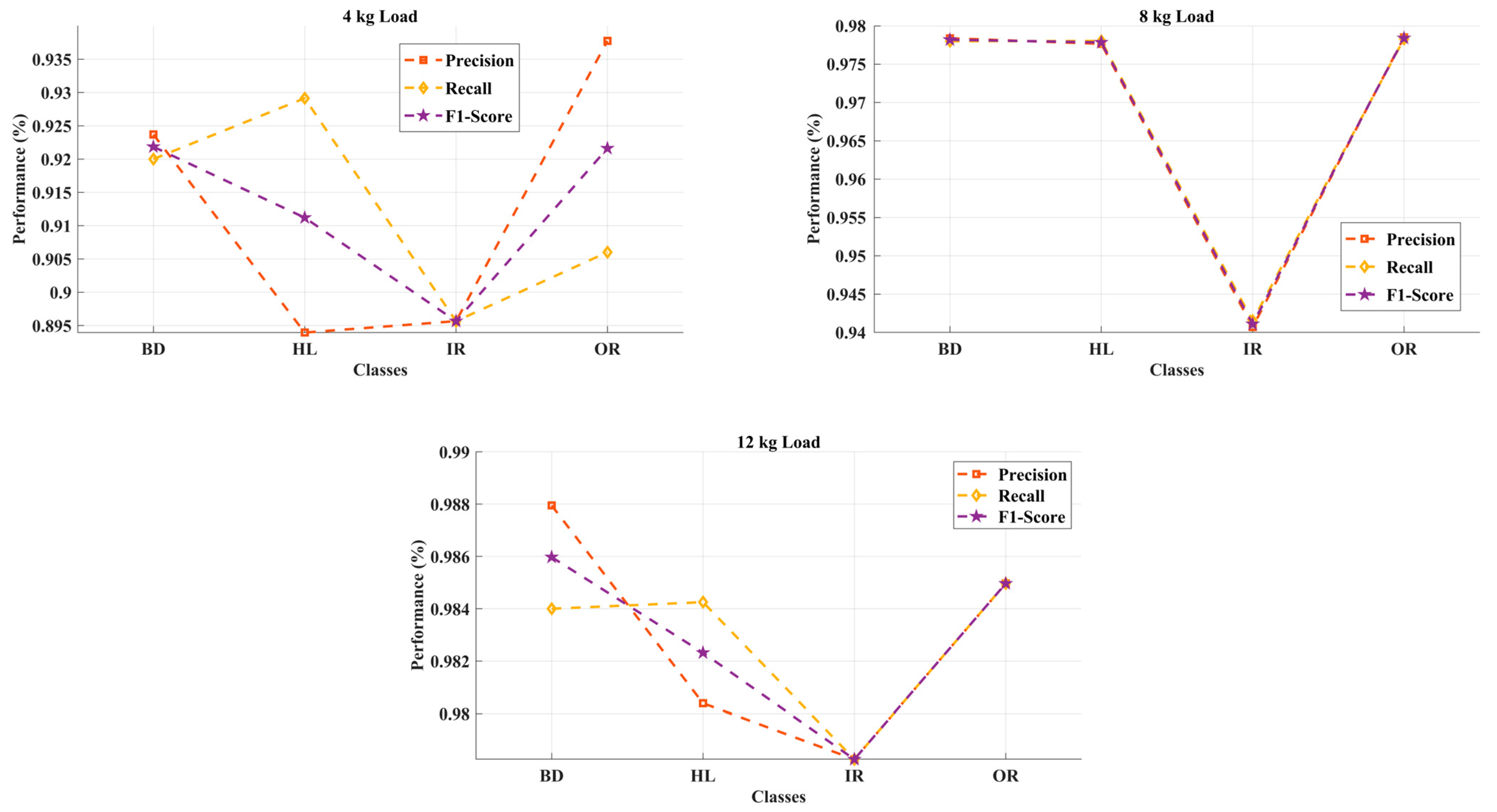
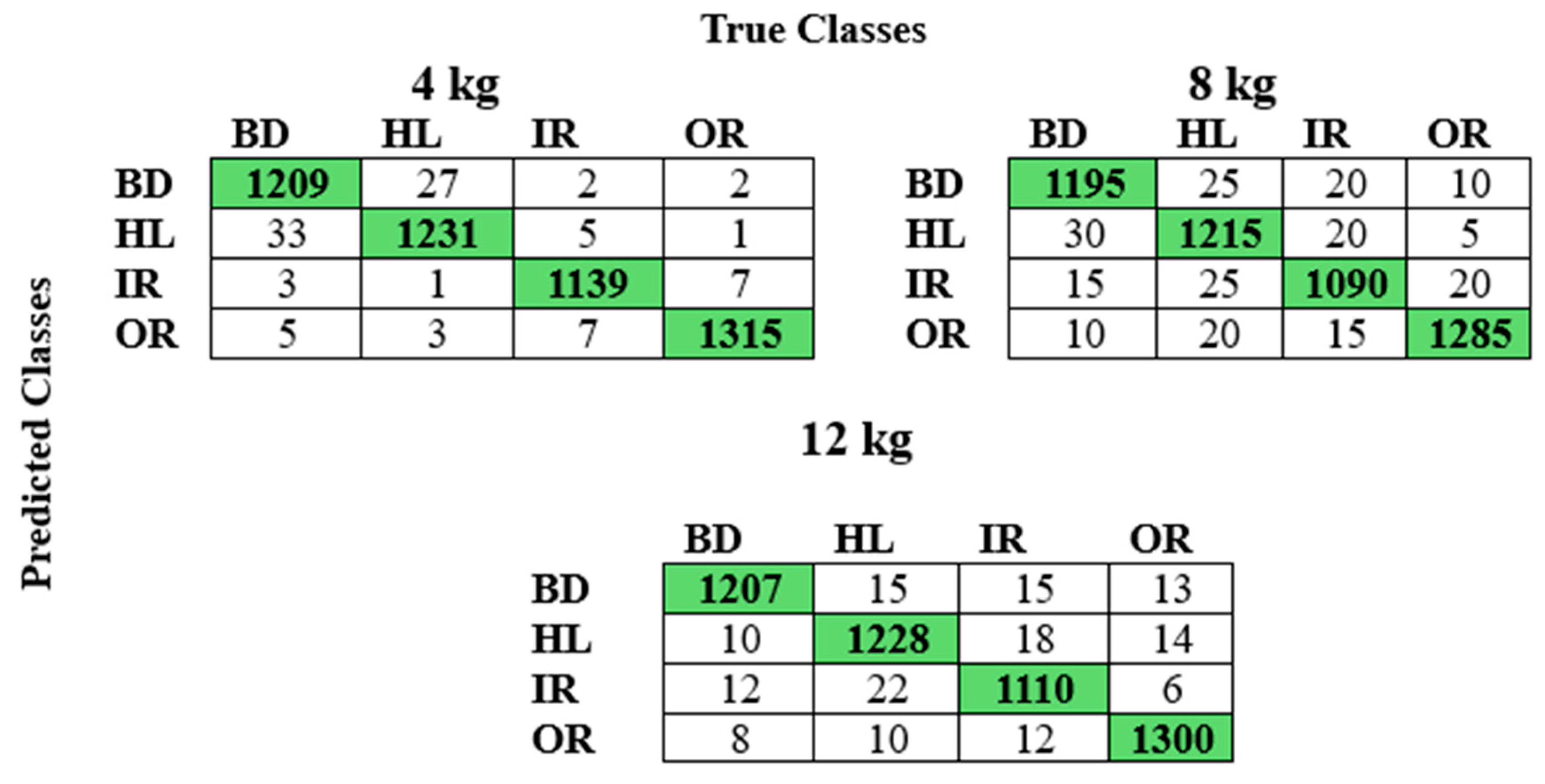
5.1. Results on Source Domain Data

Initially, a DL-based approach was applied to laboratory-based vibration data, using a CNN to build the diagnostic architecture. All extracted frames from the time–frequency spectrum have been used to train the DL model and evaluate its performance under various operating conditions, including different loads (4 kg, 8 kg, and 12 kg) at different rotating speeds (1000 rpm, 1200 rpm, and 1400 rpm). The results are presented through a confusion matrix, highlighting the model’s classification accuracy across various fault conditions, followed by performance metrics derived from it. The confusion matrix for various loading conditions is shown in Figure 8. The number of predicted samples as the true positive for individual classes is 1150 for BD, 1180 for healthy conditions, 1030 for IRD, and 1205 for ORD conditions under a 4 kg load. Likewise, the true positive samples under 8 kg conditions are 1200 for BD, 1220 for HL, 1215 for IR, and 1285 for OR. In a 12 kg load, the samples are 1230 for BD, 1250 for HL, 1125 for IR, and 1310 for OR. The confusion matrices illustrate that the model is highly accurate in identifying bearing faults at all loads. Its performance is better when the load is high, reflecting an increase in reliability at greater loads. Although it has few misclassifications, the findings demonstrate superb classification accuracy, especially at higher levels (12 kg), with classification accuracy approaching 99% for all fault types. The best performance for ORD is achieved and the greatest improvement in BD classification occurs as loads increase from 4 kg to 12 kg.

The class-wise precision, recall, and F1 score of the proposed CNN model for various load conditions (4 kg, 8 kg, and 12 kg) with a consistent rotation of 1000 rpm are shown in Figure 9. Performance metrics under the 4 kg load condition are within the range of 89.5% to 93.5%, with the ORD having the best scores due to the pronounced fault signature, while the IRD has comparatively low scores (89.5%) due to the subtle vibration characteristics under light loads. At an increasing load level to 8 kg, the model has a significant improvement with most of the classes’ performance metrics surpassing 95%. The ORD continues to have the best classification results (97.98%), while the IRD continues to have slightly less satisfactory metrics (94%), signaling consistent difficulties in separating its characteristics due to the superposition of frequency components.

With the 12 kg load, the model has the best overall performance with the values of precision, recall, and F1 score ranging from 98.0% to 98.9%. The higher load raises the fault-induced vibrations, leading to more pronounced time–frequency patterns that have enhanced separability. Despite this, the IRD is the most difficult to classify, but with significant improvement to 97.16%. These findings demonstrate the model’s resilience across different loads and confirm the effectiveness of the STFT-based CNN strategy. The trend also infers that while the overall performance is enhanced with the rise in load-induced fault excitation, some types of defects like IR have inherent classification difficulties that may demand further optimization in feature selection techniques.

At 1200 rpm, the confusion matrices, as shown in Figure 10, depict that the diagnostic system achieved accuracies around 97% for HL bearings, 98% for ORD, 96% for IRD, and 97% for BD at 4 kg load. As the load increased to 8 kg and 12 kg, the accuracies improved to roughly 98% to 99% across conditions. The confusion matrices show that misclassifications consistently decreased with increasing load, indicating clearer and more distinguishable fault signals under higher loads. These findings confirm the robustness and consistency of the FD method under varying operating conditions.

The different performance metrics shown in Figure 11 indicate that for the 4 kg load case, the model performs moderately, with measures varying from around 85% to 88%. The OR fault has the highest level of performance in this case, while the most challenging class to classify is the IR fault, which is an indication of the subtle fault-induced signal features under light loads. For the 8 kg load case, the classification performance increases for all the fault classes. The healthy class has a peak in precision, while the BD, along with the IR, faults have symmetric performances in both recall and F1 scores, at around 98% to 98.8%. This implies that moderate loads strengthen the fault signature of the vibration signal to promote feature discrimination. Under the 12 kg load case, the model performs the best for the majority of the classes with measures higher than 96%. The example of the IR fault is observed to have an enhanced level of performance in this case, indicating that high loads strengthen the fault features to a greater extent, making them more discriminable in the time–frequency plane. Slight variation among classes continues to exist due to the inherent complexities of the signal, along with the fault-specific properties. These findings affirm the model’s reliability in matching load-induced variations without compromising accuracy, emphasizing how critical the condition of loads is in enhancing fault feature strengthening for effective classification.

At a speed of 1400 rpm, the obtained confusion matrix applicable for different loading conditions is illustrated in Figure 12. At a 4 kg load, the model achieved correct classifications of 1209 for BD, 1231 for healthy, 1139 for IRD, and 1315 for ORD, with minor confusion (e.g., 33 misclassifications between H and BD). At an 8 kg load, the numbers adjusted slightly to 1195, 1215, 1090, and 1285, respectively, with a noticeable increase in misclassifications for IRD. At a 12 kg load, the results were 1207, 1228, 1110, and 1300, respectively, indicating a small overall recovery in performance. Overall, the model consistently achieves high accuracy, with ORDs being the easiest to classify and IRDs the most challenging, especially under varying loads.

The performance measures calculated from the confusion matrices obtained at 1400 rpm are shown in Figure 13, which indicates that at 4 kg load condition, the model delivers high-performance classification, where measures are well above 97% for all classes of faults. The highest scores of precision and recall around 99% are recorded for IRD and ORD, demonstrating their unique fault signatures at this load. BD and healthy classes also have good scores, though slightly less than IR and OR, due to slight difficulties in feature separability under light load conditions. With the 8 kg load, the classification accuracy is good, where the ORD has the highest measures around 97.5%. BD and HL classes have well-balanced performance, while the IRD, although with slightly less, nonetheless has measures greater than 94%, portraying enhanced detectability at higher loads. With the 12 kg load condition, the measures stabilize with a small class-specific variation. The ORD leads with respect to precision, recall, and F1 scores of around 97.8%, followed by BD, HL, and the IR classes with measures ranging from 96% to 97%. The small reduction in IR measures is a reflection of continued difficulties in the complete isolation of IR fault features, even with enhanced fault excitation at higher loads. Overall, the model is shown to have good classification capacity in all the load conditions at 1400 rpm, confirming the suitability of the STFT-based CNN model in extracting fault features with high discriminatory capacity. The patterns illustrate the positive influence of enhanced load in enhancing the classification capability, while also demonstrating the relative harshness of the detection of IRD.

Table 3. Comparison of pre-trained models based on training time and accuracy.

Pre-Trained Model	No. of Training Samples	No. of Testing Samples	Training Time (min)	Testing Time (min)	Accuracy
STFT-GoogleNet	100,000	1225	150	5	97.56
STFT-ImageNet	100,000	1225	17	6	95.45
STFT-ResNet	100,000	1225	210	6.8	97.45
Proposed	100,000	1225	75	4.3	97.56

compares four pre-trained models trained with 100,000 samples and tested on 1225 samples. Other models, including STFT-GoogleNet, STFT-Image, and STFT-ResNet, are used in a similar manner but include modifications to the classification layer to match the number of available data classes. The results obtained on the source domain dataset using the proposed approach indicate a considerable enhancement in diagnostic detection, with 97.56% overall accuracy in just 75 min of training time and 4.3 min of testing time. STFT-GoogleNet achieves the same accuracy (97.56%) but requires twice the training time (150 min). STFT-ImageNet is the fastest for training (17 min) but has the lowest accuracy (95.45%), while STFT-ResNet has the highest training time (210 min) with 97.45% accuracy.

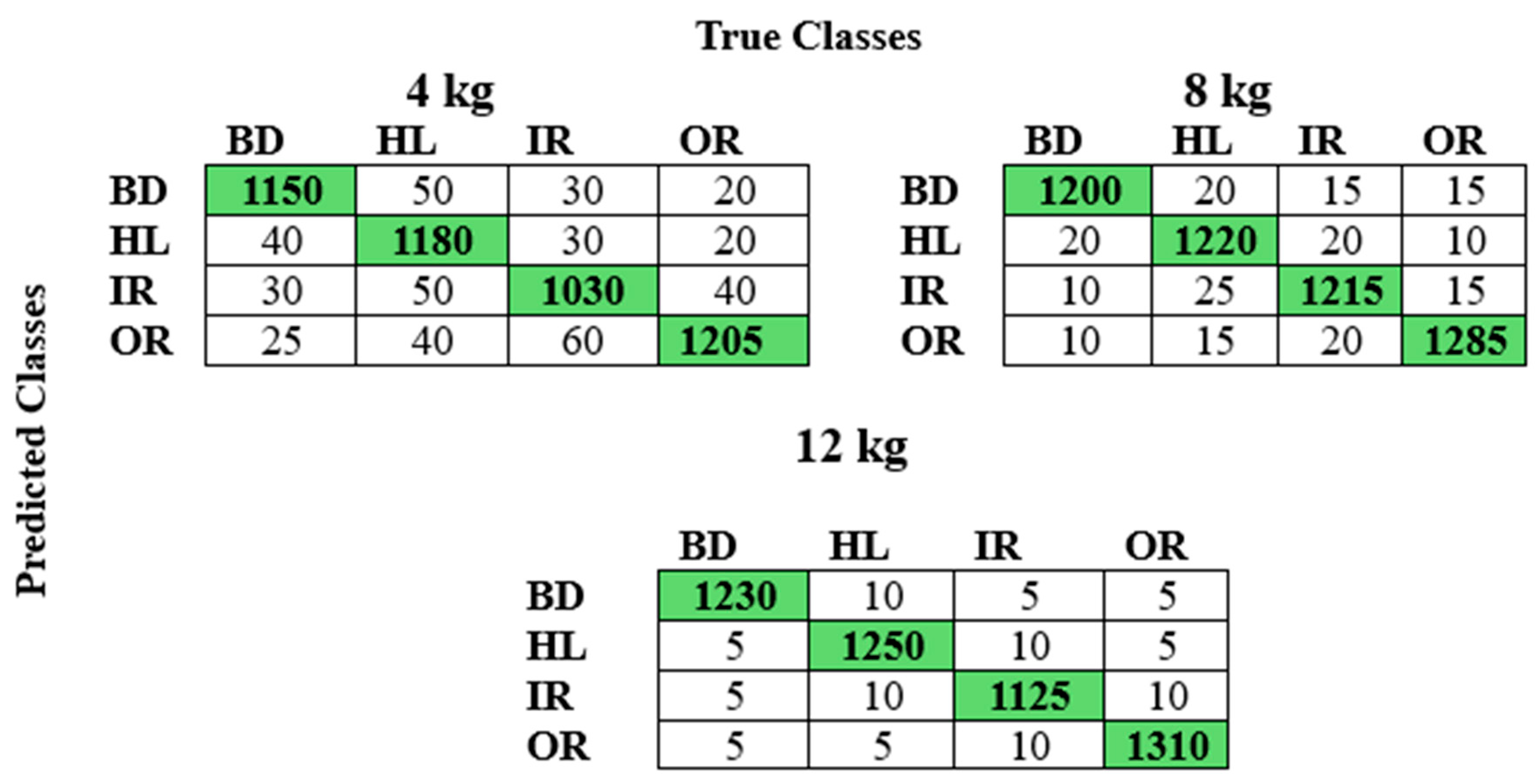
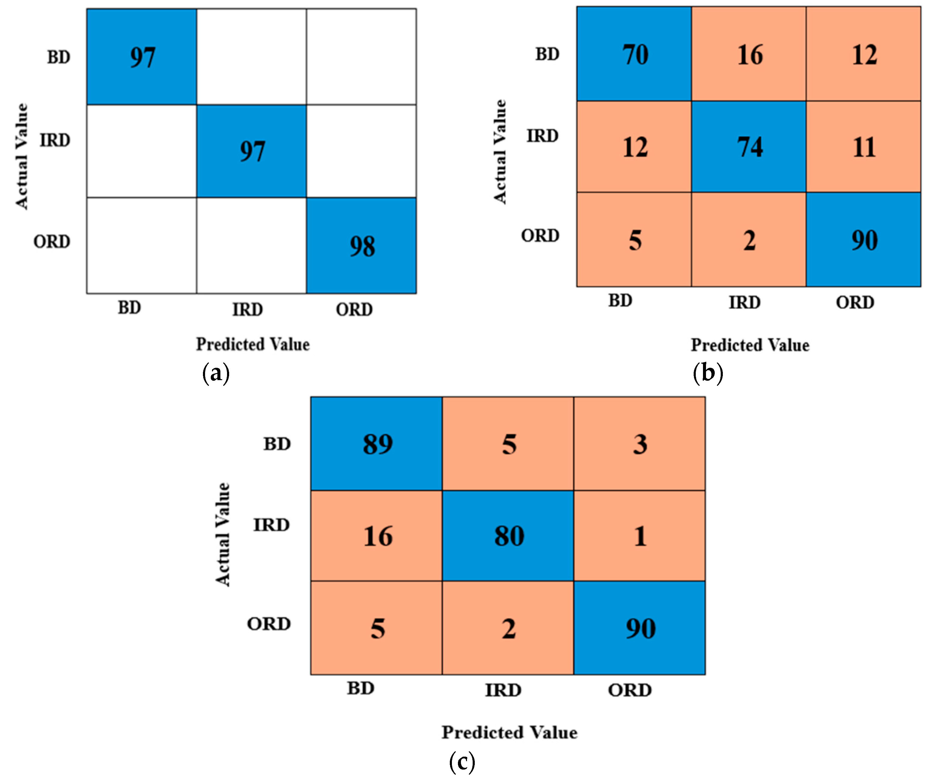
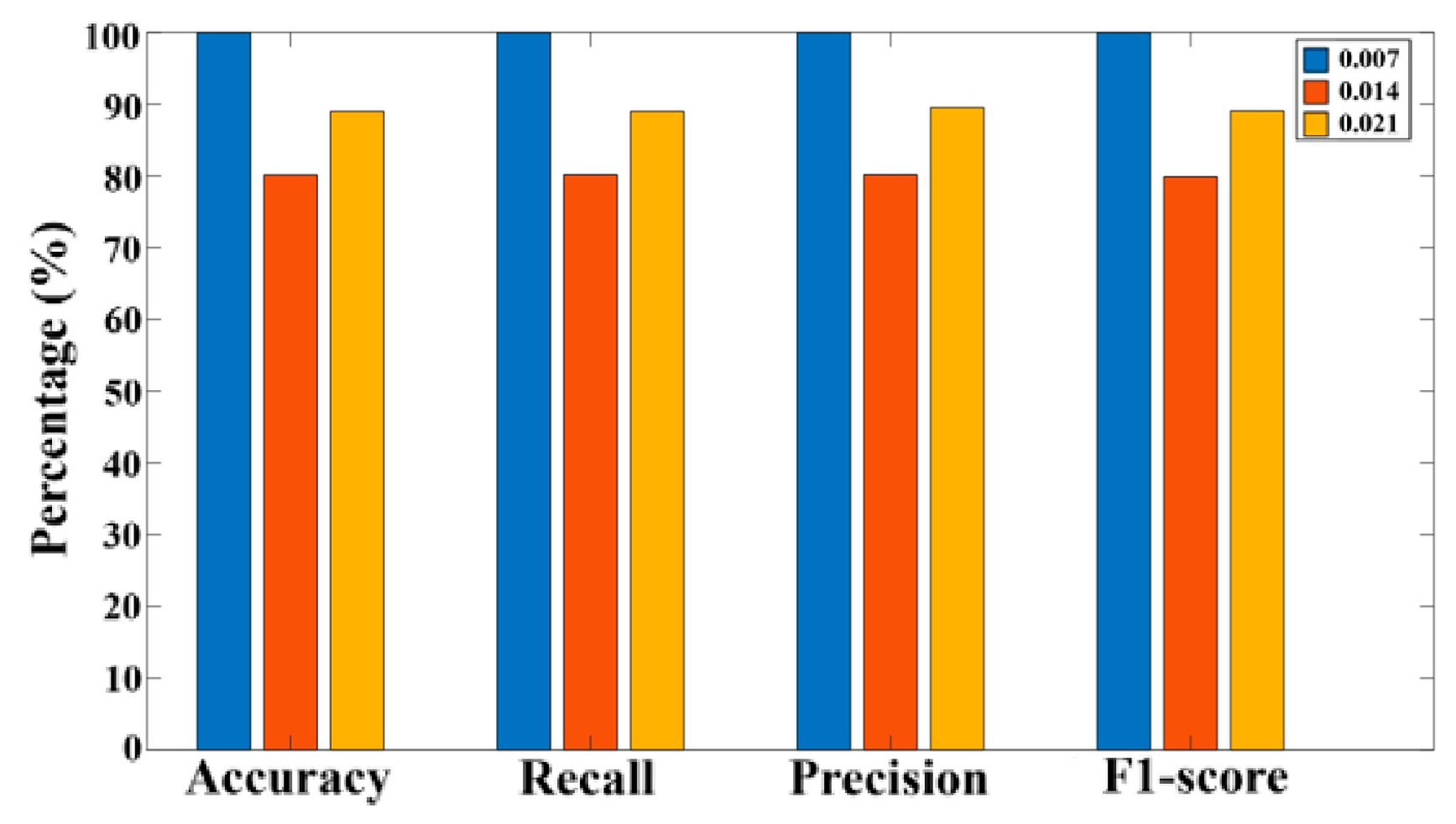
5.2. Results on Target Domain Data

To assess the performance of the proposed TL-based diagnostic approach, additional testing was conducted using datasets with potential applicability across diverse industrial environments. The proposed method proved to be robust and accurate when validated on the well-established CWRU dataset. This dataset was chosen to reflect a range of conditions, including various bearing fault types, fluctuating environmental conditions, and distinct operational environments. Thorough testing was part of the evaluation process to determine the models’ sensitivity, specificity, and accuracy under these diverse scenarios. The results consistently confirmed the model’s robustness and adaptability, maintaining a high recognition rate throughout.

CWRU Dataset

The CWRU dataset experiments utilized a 2-HP electric motor, with acceleration data collected from sensors positioned both close to and distant from the motor bearings. EDM was used to purposefully introduce faults into the motor bearings. The outer race, rolling element, and inner race were subjected to faults with diameters varying between 0.007 and 0.021 inches. After installing the defective bearings, vibration data were collected across motor loads from 0 to 3 HP and speeds between 1797 and 1720 rpm.

In the target domain method, vibration data were captured at 12 kHz and 48 kHz sampling rates during drive-end bearing experiments. The motor load is constant, with a 1 HP motor running at 1772 rpm, as used in this study. The data files are divided into three types of defects: BD, IRD, and ORD. In Figure 14, the raw data at a sampling rate of 12 kHz is presented, with faults classified into three types according to their diameters: 0.007 inches, 0.014 inches, and 0.021 inches.

Figure 15 depicts the confusion matrix on the CWRU dataset at a sampling rate of 12 kHz. The method demonstrated strong classification accuracy on the CWRU dataset. For the 0.007-inch fault, the model achieves perfect classification with all instances correctly identified (BD: 97, IRD: 97, ORD: 98). With the 0.014 inches, performance decreases, as BD is correctly classified 70 times (with 28 misclassifications), IRD, 74 times (with 23 errors), and ORD, 90 times (with 7 errors). The 0.021-inch fault condition presents normalized results to facilitate comparison across classes regardless of sample size differences. These matrices effectively demonstrate how classification accuracy varies with fault severity, with smaller faults being more challenging to classify correctly than larger ones.

Further, Figure 16 presents the performance metrics (accuracy, recall, precision, and F1 score) obtained from the corresponding confusion matrices. These measures show optimal detection capability for the smallest fault diameter (0.007 inches) with perfect 100% scores across all metrics (accuracy, recall, precision, and F1 score). As fault diameter increases to 0.014 inches, performance metrics decrease slightly to approximately 80%, and further decline to around 90% for the largest 0.021-inch fault condition. This inverse relationship between fault size and detection performance suggests that the diagnostic model is more effective at identifying smaller bearing faults in the CWRU dataset. This could be attributed to signal distortions, increased noise, or data imbalance in the dataset for larger fault conditions. These factors may affect the clarity of fault-specific features in the time–frequency domain, impacting classification performance.

To further evaluate the performance of the proposed method, it was also tested with a sampling rate of 48 kHz. As seen in the confusion matrices in Figure 17, the current model exhibits varying classification accuracy under different fault conditions. For the 0.007-inch fault, the model achieved high accuracy with 194, 193, and 194 correct classifications for BD, IRD, and ORD, respectively. The 0.014-inch fault showed moderate performance with 135, 320, and 162 correct predictions. The 0.021-inch fault exhibited the highest number of correct classifications with 532, 564, and 512 for the three fault conditions.

Further, the performance measures (accuracy, precision, recall, and F1 score) shown in Figure 18 remain consistent across the three distinct fault scenarios. For the 0.007-inch fault condition, the model achieved the highest accuracy, that is, 99.7%. This suggests that the model effectively captures and distinguishes the fault signatures associated with smaller, localized defects when provided with high-resolution time–frequency information at 48 kHz. Under the 0.014-inch fault condition, a noticeable drop in performance is observed, with metrics stabilizing around 85%. This decline may be attributed to increased complexity in signal patterns, possible overlap in frequency components, or variations in fault energy distribution, making classification more challenging. However, the 0.021-inch defect shows a recovery in performance, with metrics improving to approximately 90% across all evaluation criteria. This trend suggests that larger defects, while introducing more pronounced vibrations, produce distinct fault features that can be effectively learned by the model, though not as clearly as the smallest defect case. The non-linear relationship between defect size and classification performance observed here underscores the influence of defect-induced signal characteristics, data distribution, and model sensitivity.

Table 4. Comparison of the current study with related relevant published studies.

Ref.	Sensor Modalities	Signal Processing	Computational Method	Accuracy
				Source Domain	Target Domain
[7]	Vibration	Empirical wavelet transform	Deep adversarial TL with transferability measurement (DATLTM)	97.67%	98.68%
[36]		Continuous wavelet transform	Light-weight CNN	96.6%	98%
[9]	Vibration	-	TL + Sa-DBA	99.7%	92.48%
[4]	Thermal image	Image SNR	TL + CNN	100%	95.4%
Current study	Vibration	STFT	TL + CNN	97.56%	99.7%

compares the success rates achieved by the proposed methodology with similar published studies based on sensor modalities, signal processing, and computational methods. The current study achieves a target domain accuracy of 99.7% using vibration data, STFT for signal processing, and TL + CNN, outperforming most other studies. Mi et al. [7] achieved 98.68% target accuracy using empirical wavelet transform and deep adversarial TL. Su et al. [9] achieved the highest source domain accuracy (99.7%) but lower target domain accuracy (92.48%). Choudhary et al. [4] used thermal image data to train the TL + CNN model and achieved perfect source domain accuracy (100%) but a lower target domain accuracy of 95.4%. The superior performance on the target domain can be attributed to factors such as reduced noise, better signal quality, and more balanced class distribution in the target dataset after preprocessing. Additionally, the TL-based CNN architecture effectively adapted source domain knowledge to the target conditions, enhancing classification accuracy. Similar observations have been reported in the existing literature [7], where transfer learning improves target domain performance by mitigating domain shifts and enabling feature reuse. The results highlight that the method can diagnose bearing faults successfully and accurately using vibration signal analysis.

6. Conclusions

A vibration signal-based bearing FD approach has been proposed using TL + CNN. Experiments were carried out for different bearing conditions under varying load and speed settings. By integrating STFT, CNN, and TL, an intelligent diagnostic model has been developed to identify bearing states across diverse industrial scenarios. The method was validated using laboratory data (source domain) and CWRU dataset (target domain). The findings highlight the potential of TL to use existing diagnostic knowledge and apply it to new, unseen environments. Key outcomes from this study are as follows:

• The proposed methodology enhances FD performance with significantly reduced training time.
• The effectiveness of the proposed method has been validated using bearing datasets from rotary machinery that are entirely different from the source data.
• The method demonstrates strong capability in addressing the challenge associated with scarce training data for diagnostic tasks.

Future research may focus on extending our approach to compound or multi-FD rotary machinery under varying operating conditions. Secondly, imbalanced learning techniques could be incorporated to enhance feature learning in cases where class distributions are uneven. Thirdly, partial and universal TL frameworks can be explored for scenarios with mismatched class distributions between source and target domains.

References

1. Nguimfack, R.T.; Bappy, M.M.; Al Mamun, A.; Tian, W. Domain adaptation between heterogeneous time series data: A case study on real-time rotary machinery fault diagnosis. Manuf. Lett. 2024, 41, 1535–1543. [Google Scholar] [CrossRef]
2. Goyal, D.; Choudhary, A.; Sandhu, J.K.; Srivastava, P.; Saxena, K.K. An intelligent self-adaptive bearing fault diagnosis approach based on improved local mean decomposition. Int. J. Interact. Des. Manuf. 2022, 1–11. [Google Scholar] [CrossRef]
3. Tang, S.; Ma, J.; Yan, Z.; Zhu, Y.; Khoo, B.C. Deep transfer learning Strategy in intelligent fault diagnosis of rotating machinery. Eng. Appl. Artif. Intell. 2024, 134, 108678. [Google Scholar] [CrossRef]
4. Choudhary, A.; Mian, T.; Fatima, S.; Panigrahi, B.K. Passive Thermography Based Bearing Fault Diagnosis Using Transfer Learning With Varying Working Conditions. IEEE Sens. J. 2023, 23, 4628–4637. [Google Scholar] [CrossRef]
5. Goyal, D.; Dhami, S.S.; Pabla, B.S. Vibration Response-Based Intelligent Non-Contact Fault Diagnosis of Bearings. J. Nondestruct. Eval. Diagn. Progn. Eng. Syst. 2021, 4, 012006. [Google Scholar] [CrossRef]
6. Mehta, A.; Goyal, D.; Choudhary, A.; Pabla, B.S.; Belghith, S. Machine Learning-Based Fault Diagnosis of Self-Aligning Bearings for Rotating Machinery Using Infrared Thermography. Math. Probl. Eng. 2021, 2021, 9947300. [Google Scholar] [CrossRef]
7. Mi, J.; Chu, M.; Hou, Y.; Jin, J.; Huang, W.; Xiang, T.; Wu, D. A Fault Diagnosis Method for Rolling Bearing Based on Deep Adversarial Transfer Learning With Transferability Measurement. IEEE Sens. J. 2024, 24, 984–994. [Google Scholar] [CrossRef]
8. Goyal, D.; Mongia, C.; Sehgal, S. Applications of Digital Signal Processing in Monitoring Machining Processes and Rotary Components: A Review. IEEE Sens. J. 2021, 21, 8780–8804. [Google Scholar] [CrossRef]
9. Su, Z.; Zhang, J.; Xu, H.; Zou, J.; Fan, S. Deep semi-supervised transfer learning method on few source data with sensitivity-aware decision boundary adaptation for intelligent fault diagnosis. Expert. Syst. Appl. 2024, 249, 123714. [Google Scholar] [CrossRef]
10. Sun, X.; Wang, S.; Jing, J.; Shen, Z.; Zhang, L. Fault diagnosis using transfer learning with dynamic multiscale representation. Cogn. Robot. 2023, 3, 257–264. [Google Scholar] [CrossRef]
11. Liang, J.; Liang, Q.; Wu, Z.; Chen, H.; Zhang, S.; Jiang, F. A Novel Unsupervised Deep Transfer Learning Method With Isolation Forest for Machine Fault Diagnosis. IEEE Trans. Industr. Inform. 2024, 20, 235–246. [Google Scholar] [CrossRef]
12. Koutsoupakis, J.; Seventekidis, P.; Giagopoulos, D. Machine learning based condition monitoring for gear transmission systems using data generated by optimal multibody dynamics models. Mech. Syst. Signal Process. 2023, 190, 110130. [Google Scholar] [CrossRef]
13. Yin, Z.; Hou, J. Recent advances on SVM based fault diagnosis and process monitoring in complicated industrial processes. Neurocomputing 2016, 174, 643–650. [Google Scholar] [CrossRef]
14. Goyal, D.; Choudhary, A.; Pabla, B.S.; Dhami, S.S. Support vector machines based non-contact fault diagnosis system for bearings. J. Intell. Manuf. 2020, 31, 1275–1289. [Google Scholar] [CrossRef]
15. You, L.; Fan, W.; Li, Z.; Liang, Y.; Fang, M.; Wang, J. A Fault Diagnosis Model for Rotating Machinery Using VWC and MSFLA-SVM Based on Vibration Signal Analysis. Shock. Vib. 2019, 2019, 1908485. [Google Scholar] [CrossRef]
16. Goyal, D.; Dhami, S.S.; Pabla, B.S. Non-Contact Fault Diagnosis of Bearings in Machine Learning Environment. IEEE Sens. J. 2020, 20, 4816–4823. [Google Scholar] [CrossRef]
17. Martínez-Morales, J.D.; Palacios-Hernández, E.R.; Campos-Delgado, D.U. Multiple-fault diagnosis in induction motors through support vector machine classification at variable operating conditions. Electr. Eng. 2018, 100, 59–73. [Google Scholar] [CrossRef]
18. Zhang, J.; Zhang, Q.; Qin, X.; Sun, Y. A two-stage fault diagnosis methodology for rotating machinery combining optimized support vector data description and optimized support vector machine. Measurement 2022, 200, 111651. [Google Scholar] [CrossRef]
19. Simon, H.A. The Sciences of the Artificial; MIT Press: Cambridge, MA, USA, 1969. [Google Scholar]
20. Zhang, L.; Lin, J.; Liu, B.; Zhang, Z.; Yan, X.; Wei, M.A. Review on Deep Learning Applications in Prognostics and Health Management. IEEE Access 2019, 7, 162415–162438. [Google Scholar] [CrossRef]
21. Chen, H.; Wang, J.; Tang, B.; Xiao, K.; Li, J. An integrated approach to planetary gearbox fault diagnosis using deep belief networks. Meas. Sci. Technol. 2016, 28, 025010. [Google Scholar] [CrossRef]
22. Pan, T.; Chen, J.; Zhou, Z. Intelligent Fault Diagnosis of Rolling Bearing via Deep-Layerwise Feature Extraction Using Deep Belief Network. In Proceedings of the 2018 International Conference on Sensing, Diagnostics, Prognostics, and Control (SDPC 2018), Xi’an, China, 15–17 August 2018; pp. 509–514. [Google Scholar] [CrossRef]
23. Yang, Z.; Xu, B.; Luo, W.; Chen, F. Autoencoder-based representation learning and its application in intelligent fault diagnosis: A review. Measurement 2022, 189, 110460. [Google Scholar] [CrossRef]
24. Chen, X.; Zhang, B.; Gao, D. Bearing fault diagnosis base on multi-scale CNN and LSTM model. J. Intell. Manuf. 2021, 32, 971–987. [Google Scholar] [CrossRef]
25. Liu, H.; Zhou, J.; Zheng, Y.; Jiang, W.; Zhang, Y. Fault diagnosis of rolling bearings with recurrent neural network-based autoencoders. ISA Trans. 2018, 77, 167–178. [Google Scholar] [CrossRef] [PubMed]
26. Wei, Q.; Tian, X.; Cui, L.; Zheng, F.; Liu, L. WSAFormer-DFFN: A model for rotating machinery fault diagnosis using 1D window-based multi-head self-attention and deep feature fusion network. Eng. Appl. Artif. Intell. 2023, 124, 106633. [Google Scholar] [CrossRef]
27. Zheng, H.; Wang, R.; Yang, Y.; Yin, J.; Li, Y.; Li, Y.; Xu, M. Cross-Domain Fault Diagnosis Using Knowledge Transfer Strategy: A Review. IEEE Access 2019, 7, 129260–129290. [Google Scholar] [CrossRef]
28. Xiao, D.; Huang, Y.; Zhao, L.; Qin, C.; Shi, H.; Liu, C. Domain Adaptive Motor Fault Diagnosis Using Deep Transfer Learning. IEEE Access 2019, 7, 80937–80949. [Google Scholar] [CrossRef]
29. Guo, L.; Lei, Y.; Xing, S.; Yan, T.; Li, N. Deep Convolutional Transfer Learning Network: A New Method for Intelligent Fault Diagnosis of Machines with Unlabeled Data. IEEE Trans. Ind. Electron. 2019, 66, 7316–7325. [Google Scholar] [CrossRef]
30. Dong, J.; Su, D.; Gao, Y.; Wu, X.; Jiang, H.; Chen, T. Fine-grained transfer learning based on deep feature decomposition for rotating equipment fault diagnosis. Meas. Sci. Technol. 2023, 34, 065902. [Google Scholar] [CrossRef]
31. Wang, B.; Wang, B.; Ning, Y. A novel transfer learning fault diagnosis method for rolling bearing based on feature correlation matching. Meas. Sci. Technol. 2022, 33, 125006. [Google Scholar] [CrossRef]
32. Shao, X.; Kim, C.S. Adaptive multi-scale attention convolution neural network for cross-domain fault diagnosis. Expert. Syst. Appl. 2024, 236, 121216. [Google Scholar] [CrossRef]
33. Zhang, Y.; Xue, X.; Zhao, X.; Wang, L. Federated learning for intelligent fault diagnosis based on similarity collaboration. Meas. Sci. Technol. 2023, 34, 045103. [Google Scholar] [CrossRef]
34. Xu, S.; Ma, J.; Song, D. Open-set federated adversarial domain adaptation based cross-domain fault diagnosis. Meas. Sci. Technol. 2023, 34, 115004. [Google Scholar] [CrossRef]
35. Ditommaso, R.; Mucciarelli, M.; Ponzo, F.C. Analysis of non-stationary structural systems by using a band-variable filter. Bull. Earthq. Eng. 2012, 10, 895–911. [Google Scholar] [CrossRef]
36. Asutkar, S.; Tallur, S. Deep transfer learning strategy for efficient domain generalisation in machine fault diagnosis. Sci. Rep. 2023, 13, 1–9. [Google Scholar] [CrossRef]
Figure 1. TL-driven methodology for bearing FD presented in this study.
Vibration 08 00027 g001
Figure 2. Schematic of the proposed TL-based methodology.
Vibration 08 00027 g002
Figure 3. Experimental setup. Reproduced with permission from [8].
Vibration 08 00027 g003
Figure 4. Bearing conditions (a) HL, (b) IRD, (c) ORD, (d) BD. Reproduced with permission from [14].
Vibration 08 00027 g004
Figure 5. Raw vibration signal under different operating conditions: (a) speed = 1000 rpm, (b) speed = 1200 rpm, (c) speed = 1400 rpm.
Vibration 08 00027 g005
Figure 6. Sliding window-based STFT extraction process.
Vibration 08 00027 g006
Figure 7. Extracted time–frequency frame sample obtained using STFT on vibration signal acquired at 1000 rpm for different bearing conditions: (a) ORD, (b) IRD, (c) HL, (d) BD. The left image represents the no-load condition, while the right image represents the loaded condition.
Vibration 08 00027 g007
Figure 8. Confusion matrix obtained under 1000 rpm speed conditions.
Vibration 08 00027 g008
Figure 9. Performance measures obtained under 1000 rpm speed conditions.
Vibration 08 00027 g009
Figure 10. Confusion matrix obtained under 1200 rpm speed conditions.
Vibration 08 00027 g010
Figure 11. Performance measures obtained under 1200 rpm speed conditions.
Vibration 08 00027 g011
Figure 12. Confusion matrix obtained under 1400 rpm speed conditions.
Vibration 08 00027 g012
Figure 13. Performance measures obtained under 1400 rpm speed conditions.
Vibration 08 00027 g013
Figure 14. Raw data of the CWRU dataset under different fault conditions: (a) BD with size of 0.007 inches; (b) IRD with size of 0.007 inches; (c) ORD with size of 0.007 inches; (d) BD with size of 0.014 inches; (e) IRD with size of 0.014 inches; (f) ORD with size of 0.014 inches; (g) BD with size of 0.021 inches; (h) IRD with size of 0.021 inches; (i) ORD with size of 0.021 inches.
Vibration 08 00027 g014
Figure 15. Confusion matrix illustrating the performance on the CWRU dataset at a 12 kHz sampling frequency, under the following fault conditions: (a) 0.007 inches, (b) 0.014 inches, and (c) 0.021 inches.
Vibration 08 00027 g015
Figure 16. Performance measures on the CWRU dataset at a 12 kHz sampling frequency under different fault conditions.
Vibration 08 00027 g016
Figure 17. Confusion matrix illustrating the performance on the CWRU dataset at a 48 kHz sampling frequency, under the following fault conditions: (a) 0.007-inch, (b) 0.014-inch, and (c) 0.021-inch faults.
Vibration 08 00027 g017
Figure 18. Performance measures on the CWRU dataset at a 48 kHz sampling frequency under different fault conditions.
Vibration 08 00027 g018