1. Introduction
The response of a single-degree-of-freedom (SDOF) system with a tuned mass damper with traditional linear stiffness and a dry friction damping arrangement subjected to harmonic excitation was considered by Ricciardelli and Vickery [
1]. In the traditional Coulomb damper, the optimal solution delivered a standard response curve, which almost flat in a broad range of frequencies. However, its response became singular at resonances leading to instability or excessive vibration of the primary system. A tunable friction damper was established by Lee et al. [
2] using viscous and Coulomb elements in a parallel arrangement. It was designed to work as a friction damper while the mass slips and as a vibration absorber while the mass sticks. However, it involved a more complicated and expensive viscous component. The frictional force was coupled with the vibration amplitude. This reduced the peak amplitude, and it reduced the offsets in both the frictional force and vibration amplitude. In our turbine blade vibration simulation, these offsets are inessential to damper design. A similar report was given on dual blades [
2], with minimum coupling being applied to reduce their effects. However, these offsets are essential to actual Maxwell–Coulomb (MC) friction damper testing.
In the work of Brizard et al. [
3], a friction damper was designed and a prototype was built to reduce engine vibrations on a space launcher. The friction damper was modeled by a spring in series with a friction element. The damper prototype proved to efficiently dampen the rocket engine vibrations. The design method used for dimensioning the friction damper gave an approximation of the optimal sliding force of the damper. The adaptive friction damper prototype enables the sliding force to be adjusted by controlling the normal force. For our optimal design process, the damper spring and friction element are arranged in the Maxwell configuration similarly. However, we do not consider just the energies related to the damper. The performance of its transmissibility is one of the key factors used in our design. Its derivative at the specific level is employed to optimize its stiffness ratio as another factor. Simultaneously, its damping ratio is optimized using the force ratio between the Coulomb force and the applied force.
Research efforts have been directed toward perfecting the Maxwell-type damper arrangement in dynamic vibration absorber (DVA) research. The response of the SDOF spring mass system connected to a vibration absorber with a flexible friction damper and subjected to sinusoidal excitation was considered by Sinha and Trikutam [
4]. Its flexible friction damper was of Maxwell configuration in the two-DOF system. Meanwhile, its motion equations were derived with the Lindstedt–Poincaré (LP) method, commonly used in nonlinear vibration. As approximate one-term ODEs were derived without considering stick–slip motion cases, only simple sinusoidal motion responses were generated without stick–slip motion features. Then, they were solved numerically by an ordinary differential equation (ODE) method. The friction damper was used by Wang and Chen [
5] to reduce the maximum vibration of an engine blade. Although the harmonic balance method (HBM) is a well-known method for studying nonlinear vibration problems, generally, only a one-term approximation is proposed to study the nonlinear vibration of a frictionally damped blade. In their work, an HMB procedure with a multi-term approximation was proposed. The results showed that the steady-state response and other related behavior of a frictionally damped blade were predicted accurately and quickly by an HBM with a multi-term approximation. An accurate frictional damping loop was simulated with stick–slip motions. In this analysis, a similar turbine blade is implemented to demonstrate the correctness of the hysteresis loop generated by the central difference solution. Various unconstrained central difference search methods are developed to optimize turbine blade friction and stiffness. They are well adapted, according to the finite-difference ODE solutions.
A numerical method was developed by Hatada et al. [
6] for the dynamic analysis of a tall building structure with viscous dampers in the Maxwell configuration. Viscous dampers were installed between the top of an inverted V-shaped brace and the upper beam on each story to reduce vibrations during strong disturbances like earthquakes. A third-order differential equation was established. The computational method was formulated by incorporating a finite element of the Maxwell model into the second-order ODE of motion. Forward-difference forms of restoring force and velocity were implemented to approximate its solution. Bhaskararao and Jangid [
7] investigated the dynamic behavior of two identical adjacent structures connected with viscous dampers under base acceleration. Peak displacements and minimum inter-story damping were obtained. Closed-form expressions for the optimum damping of undamped structures were applied to the damped structure. The governing differential equations of motion of the coupled system were derived and solved for relative displacement and absolute acceleration responses by Patel and Jangid [
8]. Parametric study was conducted to study the influence of important system parameters (such as excitation frequency, mass ratio, and stiffness ratio) on the response behavior of damper connected structures. Chen and Wu [
9] investigated the seismic performance of two adjacent towers and podiums connected by viscous dampers. Three types of damper placement were discussed, including installing dampers within a single building, connecting two buildings at the same floor level, and connecting two buildings at the inter-story level. In this effort, the Maxwell–Coulomb damper is applied to suppress the maximum displacement of adjacent towers and podiums subjected to ground motions. Its performance is compared with viscous damper using equivalent damping ratios.
In this SDOF design, we discover that the commonly used viscous damper is less effective for lower range damping ratio application. From the shape of contour graph, it appeared to produce straight lines. On the other side, the Maxwell–Coulomb damper displays a concave downward contour as the damping ratio decreases. Compared to the viscous damper, its performance is better at lower range. Thus, this damper can be a better alternative than the viscous damper because of its low cost and ease of maintenance. However, the friction damper was not as commonly used as viscous damper because its design involved nonlinear dynamics analysis. Also, the pure Coulomb friction damper had the problem of zero or little damping effect on the vibration of a spring–mass dynamic system at resonance where singularity is occurring. With the combination of a Maxwell spring, these gaps can be addressed by a relatively convenient conversion using a viscous equivalent damping coefficient, resulting in less drastic and more stable motion under additional stiffness.
A mesh-free least-squares-based finite difference method was applied by Wu et al. [
10] for solving the large-amplitude free vibration problem of arbitrarily shaped thin plates. Spatial derivatives of a function at a point are expressed as weighted sums of the function values of a group of supporting points. A string/slider nonlinear coupling system with a time-dependent boundary condition was considered by Fung and Chang [
11]. The finite difference method with a variable grid was employed to show the numerical results of the coupling effect between the string and slider. The three-dimensional dynamics of long pipes towed underwater were analyzed by Kheiri et al. [
12]. In their finite difference scheme, partial differential equations of motion and boundary conditions were converted into a set of first-order ODEs. In our analysis, ODEs from four case models were solved separately using the central difference method. Then, they were sequentially connected by initial displacements and velocities.
4. Experimental Validation and Optimal Design of Prototype Damper
A vibration test is carried out on the prototype damper system to experimentally validate the previous analysis, with
and
at frequency
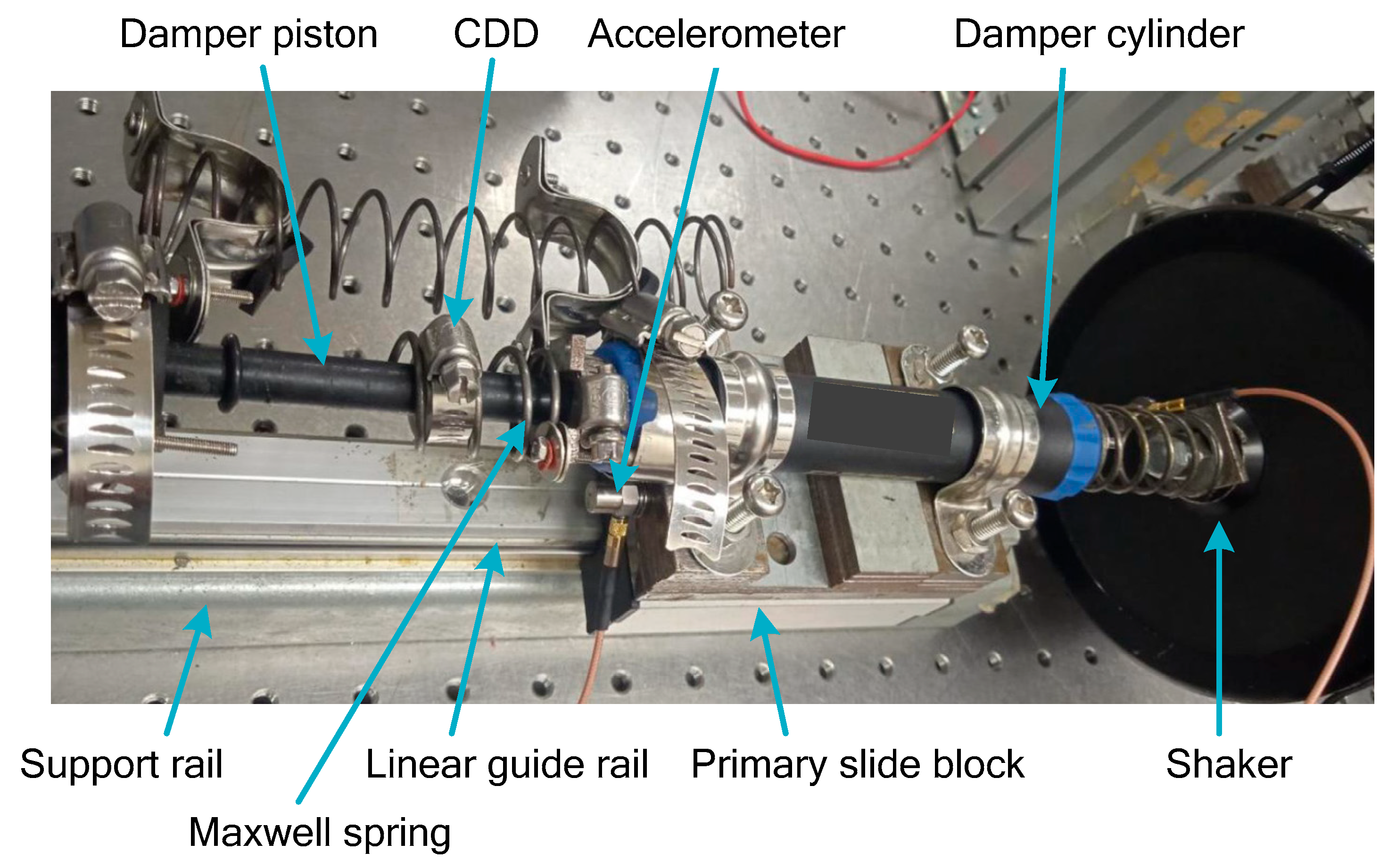
, a condition that is very close to its resonance. The prototype is of a piston–cylinder type, which is well connected to the adjustable Maxwell spring and Coulomb damping device (CDD) [
15]. A linear slide block platform is established for the linear horizontal motion of this system, consisting of slide blocks, a linear guide rail, and a support rail, as shown in
Figure 12.
Excitation force is transmitted from the shaker to structural system through the shaker spring:
where
y is the shaker displacement,
is the shaker spring stiffness, and
y −
x is the shaker–damper relative displacement. An equipment schematic of the prototype test is illustrated in
Figure 13. Vibration signals on slide block and shaker are captured by accelerometers. These signals are conditioned at the spectrum analyzer.
A Coulomb damping test is conducted by increasing the angle of the Coulomb damping device (CDD) from 90°, to 180°, to 270° in three coil tests.
[1.15, 1.36] increases, as illustrated in
Figure 14. This leads to an increase in hysteresis loop energy from 0.0190 J, to 0.0317 J, to 0.0369 J. This trend is consistent with the decrease in
, as seen in
Figure 5,
Figure 9, and
Figure 14. The slope angle of its principal axis ranges from 39.9° to 40.5°. Deviations are small, only within 1.8%. Since there is no change in
, its slope basically remains the same as in
Figure 3. The Coulomb damping ratio of the CDD is calculated by
. In case
B of forward motion, the coupling ratio [
14] between displacement and normal force increases with
. This leads to an increase in loop gradient. Similar findings are recorded in case
D of reverse motion. However, the gradient becomes saturated at
. In the shaking table test of Brizard [
3], their gradients increased continuously. Meanwhile, straight bounds on the displacements were generated, indicating high Maxwell spring stiffness in the hydraulic jack.
Using the hysteresis loops in
Figure 14, the fastening screw tuning the Coulomb damping angle
is related to
, with Coulomb angle factor
and residual damping force
:
In this line fitting of the Coulomb force test, the line slope = 6.81 × 10⁻³ N/degree and the line constant . Meanwhile, hysteresis loops at medium = 180° from the CD simulation and experiment are compared in the figure, as they represent the common experimental features. From this comparison, their motions are seen to be close to each other. Simulation loop energy 0.0317 J displays a 5.11% deviation from the experimental value. For the Coulomb damping force, is found in the simulation, which is 8.8% deviated from the experimental measurement. Compared to the experimental sliding motions under this force, they are slightly inclined. This is caused by the flexural stiffness of the rubber friction plate inside the CDD.
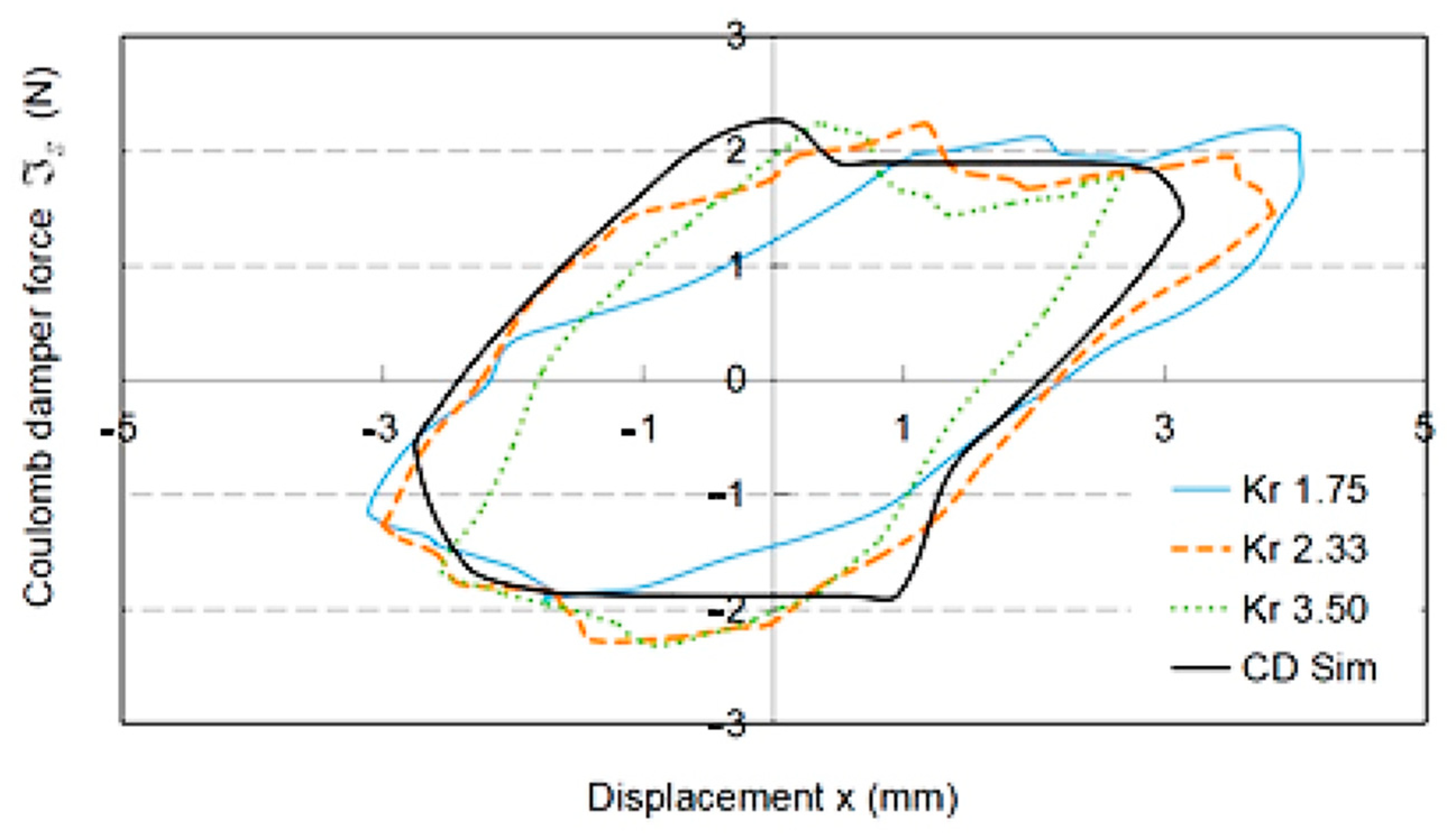
On the other hand, in the Maxwell spring test, one can decrease the Maxwell spring coil number from 4, to 3, to 2 (which is 7 in
K with same helical spring dimensions), i.e.,
[1.75, 3.50], while keeping the Coulomb device at 90°. It is interesting to note that hysteresis loop energy H
Kr decreases from 0.0776 J, to 0.0387 J, to 0.0214 J, as shown in
Figure 15. This is caused by the well-tightened joint and lessened coupling effect in the CDD. Simultaneously, the slope angle of its principal axis increases from 31.7°, to 37.8°, to 48.5°. From
Figure 3, the theoretical slope angle
is computed as
For this spring–mass system, the theoretical are 32.7°, 40.6°, and 52.1°, respectively. Compared with the experimental , their percentage errors are 3.24 to 7.58%. Hence, is validated using Equation (51). The next step is to compare the CD solver with the simulation using the experimental data. From hysteresis plot of three coils test in the figure, one discovers that both loops are well matched. The simulation is 36.5°, with a 3.4% error from the experimental . Meanwhile, HKr = 0.0375J, which is only 3.1% deviated from the experimental result.
Taking even-interval tests of
and Maxwell spring coil number, their experimental
record is obtained. The corresponding values in
are computed using the line fit of Equation (50). Meanwhile,
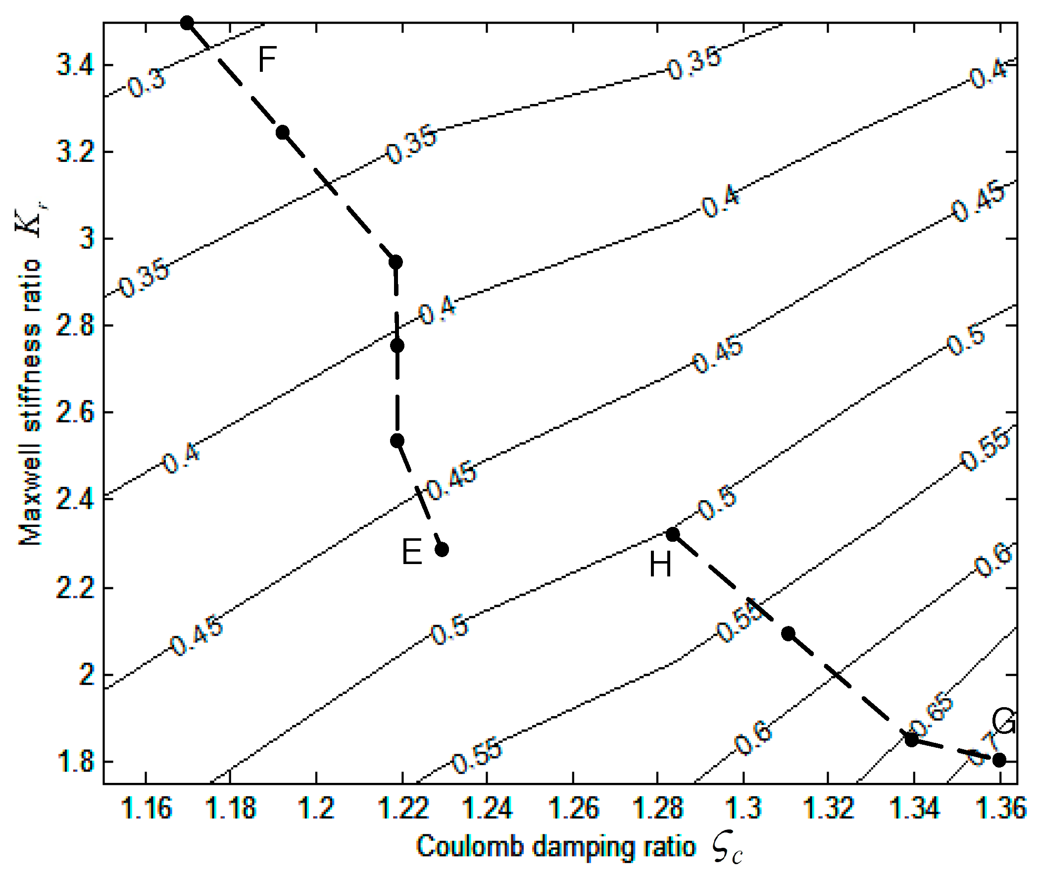
Kr are computed using the coil numbers of Maxwell spring. Inputting this record into our self-developed MATLAB program generates the experimental contour plot shown in
Figure 16.
To check the applicability of this plot in local ranges [1.15, 1.36] and [1.75, 3.50], design paths are established using CDNS. In the lower range of , the first design path starts from E, where = 0.465. A Maxwell three-coil spring is used, with a stiffness ratio of = 2.33. Meanwhile, is turned to 135°, and = 1.23, as obtained by Equation (50). Using the CDNS approach, its design path is shown as the dotted curve with black circles from E to F. It converges from E in five steps to F, with = 0.292 bounded at a two-coil spring, with = 3.50. is minimized to 100°, with = 1.17. Reduction in is 69%. Due to the constant curvature of the contour in separate ranges, the pattern of varies linearly. Meanwhile, increases vigorously from −21.0 to −2.74, indicating that the increase is significant. Hence, the CDNS approach is accurate and effective in these experimental ranges.
For a second design path in the upper range of
, as shown by the dotted curve from G to H, it converges from G, where
= 0.707 at the four-coil spring, with
= 1.80.
is at 270°, with
= 1.36. It is bounded at H at the third step, with
= 0.515, where
= 2.33 for the three-coil spring.
is minimized to 215°, with
= 1.32. Ultimately,
is reduced 27%. From the analytical solution given by Equation (31), its contour decreases monotonically from 0.75 to 0.35. In comparison with the experimental contour seen in
Figure 16, it is also monotonic, decreasing from 0.65 to 0.40. Hence, the experimental contour is closely correlated.


 ) and (
 ) of turbine blade at λ = 1.0.
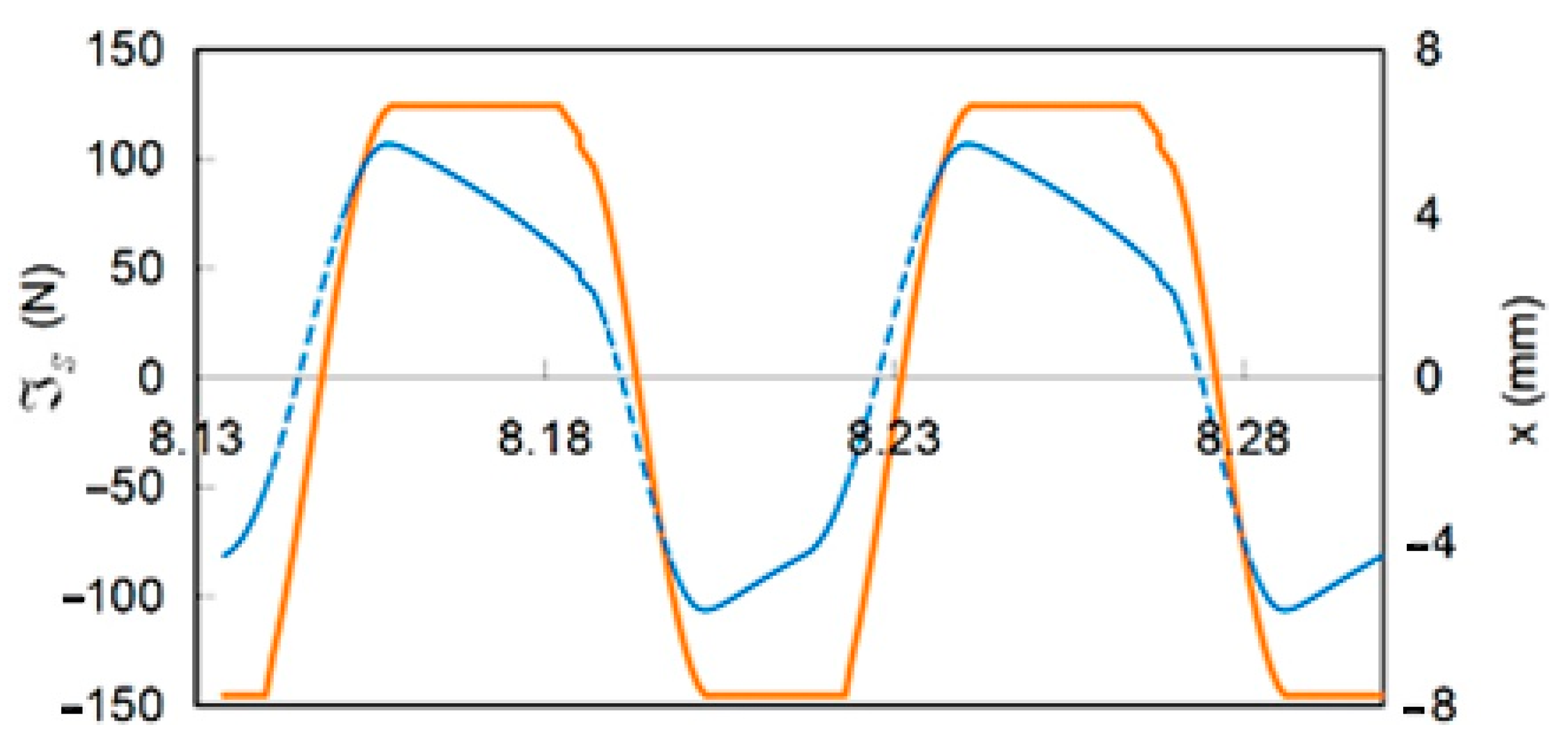


