Comparative Study of Different Linear Analysis for Seismic Resistance of Buildings According to Eurocode 8

Abstract

Structural design in Europe should strongly follow EN 1998-1 or so called Eurocode 8 (EC8), for a seismic resistance assessment of structures. Eurocode 8 recommends two linear methods and two nonlinear methods. The nonlinear methods require some knowledge about the nonlinear behavior of beams and joints in the structure, which makes the linear methods preferable. An alternative method of the seismic loading representation is to use artificial accelerograms with the same or similar spectra as the response spectrum used for modal spectrum analysis. Using an artificial diagram, three approaches in finite element methods exist: explicit time integration, implicit time integration, and modal dynamics. A typical six-story steel structure is modeled using the finite element method, and all linear methods are examined in both horizontal directions. The structure is examined by the modal response spectrum method using sufficient modes, as well as with and without the residual mode. The results are compared, and conclusions concerning the efficiency and precision of methods are deduced. Time history loading by accelerograms reveals higher dynamics and stress in the structural response than the modal response spectrum and lateral forces methods. The time history analysis methods have almost no difference in accuracy, and the modal dynamics method is the cheapest one.

1. Introduction

The assessment of seismic resistance of buildings is very important at the stage of their design in order to prevent loss of life in earthquake events. The methods of such an assessment are computational by modelling and applying the finite element method for analysis and simulation. The seismic loading can be presented in two ways [1]. One is to use the response spectrum as a generalized characteristic of the earthquake ground motion, accounting for the hazard level. The other one is by accelerograms, which can be real, recorded, and scaled to the hazard level of design or artificial accelerograms having frequency characteristics, corresponding to the response spectrum of the seismic demand.

There are four fundamental methods of seismic analysis: linear static, linear dynamic, nonlinear static, and nonlinear dynamic methods. All of them are included in the Eurocode 8 (EC8), and the linear dynamic “Modal response spectrum analysis” is pointed out as a reference method [1]. Structural engineers could choose one or two methods to provide the seismic requirements, but they are not well acquainted with the accuracy of the seismic analysis methods, as well as the computational methods and their computational costs. The purpose of this paper is to facilitate the designer’s choice of a seismic analysis method and the computational approach, as well as to contribute to the practical use of EC8.

The linear static method of analysis, described in EC8, is the “Lateral force analysis”. The method is approximate and well described in classical textbooks [2]. The structure is modeled as a Single Degree of Freedom (SDOF) mechanical system, and the total inertia force corresponding to the base shear force is calculated by taking 85% of the total mass of the structure for tall buildings, which is an approximation of the fundamental mode mass participation. Then the force is distributed proportional to the fundamental mode displacements or to the height of the stories, which is also an approximation. The lateral force method should give good results when the structural dynamic behavior is governed by the fundamental mode shape vibrations.

The linear dynamic method, proposed to model the structure as a Multi Degree of Freedom (MDOF) mechanical system, is the “Modal response spectrum analysis”. The method uses each separate mode peak response as an SDOF system response [2,3], and then the total peak response is calculated by means of one of the methods: Square Root of Sum of Squares (SRSS) or Complete Quadratic Combination (CQC). They are not theoretically justified, and some other methods for modal combinations have been proposed in the past [4,5], in order to solve problems with some type of structures, like flexible structures, for instance. The CQC method is considered superior to the SRSS method, especially when the structure has close natural frequencies [1]. Acceleration response spectra are proposed by EC8 as types, but the national annexes determine their parameters. Although the national annexes should cover the regional-specific parameters of the response spectra, it is possible to seek a site-specific response spectrum [6].

When modal analysis is used, the problem of how many modes should be taken arises. The EC8 has minimum requirements for the number of modes. Because the truncation of modes leads to a loss of mass, some methods are proposed to compensate for the missing mass [2]. According to [7], the most efficient method, however, is to add the residual mode [8].

The nonlinear methods applied for seismic analysis require a finite element model of the structure with special elements in the right places. The elements could be beams with distributed plasticity or plastic hinges [9]. The material nonlinearity is the essential part of the nonlinear methods, because the ductility of the structure should reveal its higher capacity to withstand strong ground motion. The geometrical nonlinearity is well provided by the corotational method [10], since the building structures are mainly moment-resisting frame structures, and beam and shell finite elements are used to model them. The plastic behavior of the frame structures, however, is not so easy to model. The structure joints are stiffer than they are modeled, so the right place of hinges is a little bit far from the nodes of finite element connections and depends on the joint structure in detail [11]. In order to do nonlinear analysis, one should know the nonlinear behavior of all elements of the structure, and the nonlinear model should represent that behavior with fidelity.

The nonlinear static analysis is known as pushover analysis. The methods of pushover analysis became popular because of their simplicity and low computational costs. The method implemented in EC8 is the N2 method [12]. The pushover analysis considers a monotonic loading of the structure model by lateral forces till the collapse, and the total base shear force versus the displacement of a control point (at the roof) gives a curve called the capacity curve, which could be compared with the seismic demand. The distribution of the forces is not theoretically justified, and EC8 recommends two distributions: proportional to the mass and a constant acceleration, and proportional to the mass and the first mode displacement. The structure is adjusted to an SDOF equivalent mechanical system. A target displacement is determined for the equivalent system by using the elastic response spectrum. The worst results for the structure from both force distributions, comparing the target displacement and the maximum displacement of the control point, will give the final assessment of the structure’s capacity. In fact, EC8 refers to the pushover method as a means to determine and revise the overstrength ratio and behavior factor in order to use them in a linear seismic analysis. The uncertainty in load distribution and the use of an equivalent SDOF model of the structure show that the method is approximate and not always adequate [13]. Some improvements of the method are proposed [14], and many researchers advocate nonlinear dynamic methods to replace the pushover analysis [15].

The nonlinear dynamic seismic analysis uses accelerograms to load the structure and to simulate the time history response of the structure. The finite element model should not simply have adequate elastic–plastic elements, but it should also have adequate hysteresis in the reverse cyclic loading. If the joints of the structure have an unknown hysteretic behavior, special research should be carried out [16]. Some nonstructural elements as some claddings, could have a significant contribution to the energy dissipation during a strong ground motion and also should be included in the nonlinear finite element model [17]. The development of an adequate nonlinear finite element model of structures for dynamic analysis is not a task for structural engineers in design practice, and it is more suitable for structural engineers in science.

The earthquake accelerograms used for the dynamic loading of building structures have to satisfy a lot of requirements in order to be representative of the seismic design. The recorded accelerograms could be used, but they should be scaled to the level of the regional seismic hazard. Their spectral properties could be very different from the proposed response spectrum, so the records should be selected in order to satisfy the seismic demand to be spectrum compatible [18,19,20]. An alternative to using the code spectrum is to apply the conditional mean spectrum methodology to select accelerograms [21,22]. The artificial earthquake accelerograms have become very popular recently. They can be fully synthetic, based on some seismological model and a stochastic procedure [23], or the stochastic procedure can use natural accelerograms [24,25]. The aim of the artificial accelerogram generation is to have some spectrum compatibility, but still a great variability in the time history. The generation of three-component artificial accelerograms [26] could allow more realistic simulations of seismic events. The EC8, however, recommends separate directions of the loading and combinations of them. The number of time history nonlinear dynamic analyses is recommended to be a minimum of seven in one direction of loading with different accelerograms, and the response quantities are to be averaged. If less time history analyses with different accelerograms are used, the maximum response of them is used for the design. Considering the ground-motion representation, the EC8 recommends at least three accelerograms to be used [1].

The dynamic simulations of a structural response to seismic loadings by accelerograms can be completed by a direct explicit time integration of the differential equation of motion [27,28], by a direct implicit time integration method [28], or by a modal model of the structure and modal equations of motion time integration [29]. The time integration of equations of motion requires a significant computational time and a powerful computer capability. The transient modal dynamics method is a linear dynamic method, but it can reveal some torsional behavior of the structure [30], as well as all other time integration methods applied to linear finite element models of the structure. The explicit time integration method is popular for solving impact problems, where a high geometrical and material nonlinearity exists, like crash simulations. It has great computational costs because of the small time steps of the numerical integration, and it is applied for short-time transient problems with single-precision calculations. The implicit finite element method for nonlinear problems works with double precision and has great computational costs for one step of the nonlinear problem solution but could have larger time step for the numerical integration of dynamic problems. The material nonlinearity of the finite element model could cause the implicit method to have slow convergence or even divergence [31]. This can be seen when the method is applied as a static nonlinear method for a pushover analysis. The softening of the structure as a result of the plasticity reduces the tangential modulus of elasticity and could increase the critical time step for the explicit time integration.

The aim of this research is to compare different methods of finite element analysis, described in EC8, in order to estimate their effectiveness and accuracy. The finite element model should be linear, in order for the methods of analysis to be comparable and useful for the design practice. The accelerograms used for seismic dynamic simulations should be easily available to the structural designers.

2. Methodology

2.1. Artificial Accelerograms

The artificial accelerogram should correspond to the response spectrum of the earthquake. The generator of the accelerograms, which is used here, is an available MATLAB^® 2017b version script well described in [32]. The generation of the artificial accelerogram is based on the real records of accelerograms of the following earthquakes:

• ElCentro Earthquake (1940);
• Gebze Earthquake (1999);
• Mexico City Earthquake (1985).

The original records are scaled to the level of the maximum acceleration chosen as a reference, and in this case, it is $a_g=0.15 g=1.4175$ m/${\mathrm{s}}^2$, using the coefficient of importance ${\gamma }_I=1.0$ for ordinary buildings. The response spectrum chosen is the elastic spectrum, which is recommended in EC8 for earthquake type 1, soil type C and damping ratio of response $\zeta =5\%$. The response spectrum parameters are given in

Table 1. Response spectrum parameters.

S	${\mathit{T}}_{\mathbf{B}} \left(\mathbf{s}\right)$	${\mathit{T}}_{\mathbf{C}} \left(\mathbf{s}\right)$	${\mathit{T}}_{\mathbf{D}} \left(\mathbf{s}\right)$
1.15	0.2	0.6	2.0

.

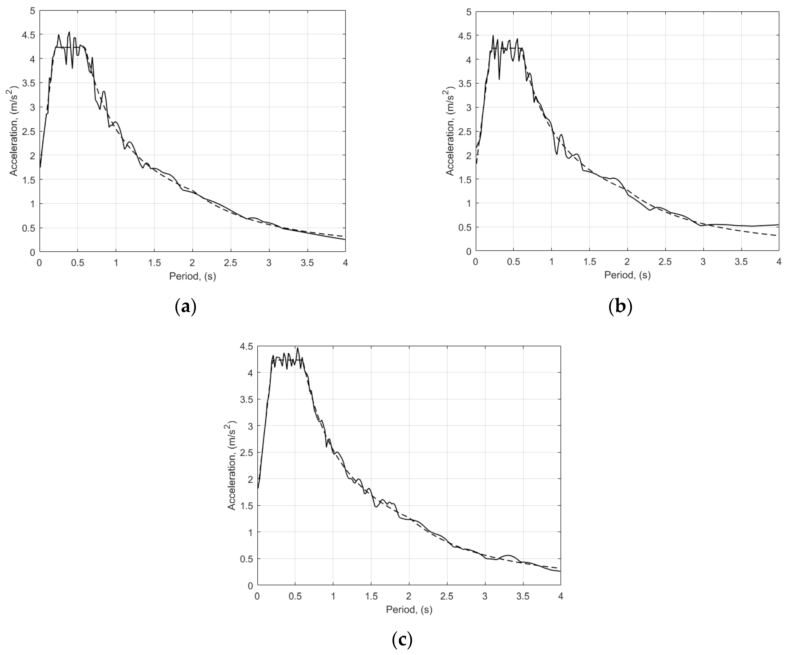
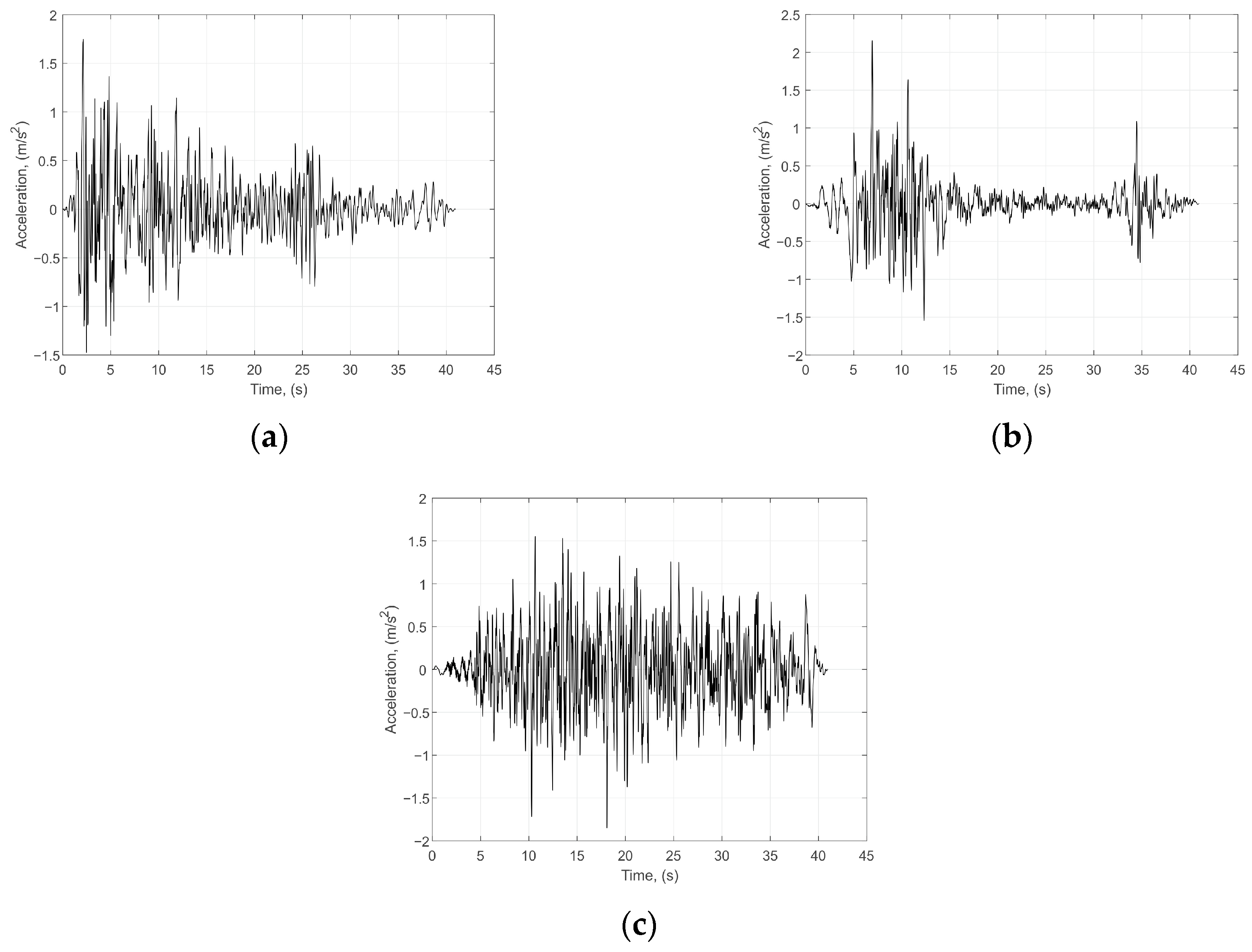
Three accelerograms are generated, corresponding to the earthquakes numbered above, and they are filtered in 8 iterations in order to be close to the chosen spectrum [6]. The correspondence of the generated accelerogram spectra to the reference spectrum can be seen in Figure 1. One can see that the artificial accelerograms are a very good match for the response spectrum. The generated accelerogram are given in Figure 2. The time of accelerograms is trimmed at 40.96 s with a time step $\mathrm{d}t=0.005$ s which means 8192 points $=2^{13}$. The number of sample points should be some power of 2, in order for the Fourier transformation to be completed. When the accelerograms are generated, then the simulations of structure loading and response can be truncated up to any time less than 40.96 s. For the purpose of the structure dynamics simulations, the time of simulations is set to be 40 s, and the number of sample points of the ground motion acceleration is $n_s=8000$.

2.2. Time History Analysis

The solution of the dynamics of structure problem by accelerograms is found by direct time integration of the differential equation of motion for finite element model of the structure:

$$\mathbf{M}\ddot{\mathit{d}}+\mathbf{C}\dot{\mathit{d}}+\mathbf{K}\mathit{d}=\mathit{f},$$

(1)

where M, C, and K are the mass, the damping, and the stiffness matrices, respectively. The nodal displacements, $\mathit{d}$, are the unknowns as a function of time, $t$, while the external nodal force vector, $\mathit{f}$, is the inertia force vector, which components are:

$$f_i=r_i m_{i}a\left(t\right) , i=\mathrm{1,2}, \dots , N_{\mathrm{D}\mathrm{O}\mathrm{F}}$$

(2)

where $r_i$ is 1, if it is in the direction of seismic loading or 0 otherwise. Here $m_i$ is the lumped translational nodal mass and $a\left(t\right)$ is the acceleration at time, $t$, taken from the accelerogram, $N_{DoF}$ is the number of the Degrees of Freedom (DOF) of the finite element model of the structure.

2.2.1. Implicit Time Integration Method

The time domain is discretized in time steps, $\mathsf{\Delta }t$, and (1) holds at any time $t_n$ for step number $n$. There are two methods of time integration of (1): implicit and explicit. The implicit time integration can be expressed in this way:

$${\mathit{d}}_{n+1}=f({\dot{\mathit{d}}}_{n+1},{\ddot{\mathit{d}}}_{n+1}{,\mathit{d}}_n,\dots )$$

(3)

which should be read as find the displacements at $n+1$ time step as a function of the velocity and acceleration at the same time step plus all that is known from previous steps. The implicit method is unconditionally stable, so the time step, $\mathsf{\Delta }t$, could be any, but small enough in order to capture the dynamics of the structure. This is why we will solve the equation of motion with implicit method in 8000 increments (time steps). The great problem of the method is that a system of linear equations should be solved at each time step or iteration, which is time consuming calculations especially for large model with a lot of DOF.

2.2.2. Explicit Time Integration Method

The explicit method of time integration can be summarized in this way:

$${\mathit{d}}_{n+1}=f({\mathit{d}}_n,{\dot{\mathit{d}}}_n,{\ddot{\mathit{d}}}_n,{\mathit{d}}_{n-1},\dots )$$

(4)

Using lumped mass matrix and lagging the velocity in a half step behind leads to that all internal and viscous forces depending of displacements and velocities are known from the previous time steps, and only nodal accelerations should be determined for the current time step, ${\ddot{\mathit{d}}}_{n+1}$, then it is easy to find the velocities, ${\dot{\mathit{d}}}_{n+1/2}={\dot{\mathit{d}}}_{n-1/2}+\mathsf{\Delta }t {\ddot{\mathit{d}}}_{n+1}$, and the displacements, ${\mathit{d}}_{n+1}={\mathit{d}}_n+\mathsf{\Delta }t {\dot{\mathit{d}}}_{n+1/2}$, node by node. The solution of the equation of motion in the time steps consists of nodewise and elementwise cycles of calculations without any linear equation system solution. This makes time step calculations very fast and efficient, however the method is conditionally stable.

The condition for stability of the time integration is that the time step should be:

$$\mathsf{\Delta }t\le {\displaystyle \frac{2}{{\omega }_{\mathrm{m}\mathrm{a}\mathrm{x}}}} , {\omega }_{\mathrm{m}\mathrm{a}\mathrm{x}}={\displaystyle \frac{2c}{L_{\mathrm{m}\mathrm{i}\mathrm{n}}}}$$

(5)

where ${\omega }_{\mathrm{m}\mathrm{a}\mathrm{x}}$ is the maximum angular frequency of the discretized structure, which is determined by the element with a high sound speed, $c$, and a small minimal distance between its nodes, $L_{\mathrm{m}\mathrm{i}\mathrm{n}}$. This condition depends on the degree of discretization of the structure and makes the time step very small. The problem is solved on the level of tracking mechanical waves, which means it makes real life simulations of mechanical interactions and dynamics.

The number of increments in time could be very high. When it is comparatively small, as in the case of very short transient events as impact simulations or explosion simulations, a single precision is used in the computer calculations, which makes the problem solution quite acceptable. However, for a time of event as 40 s, which we have for time history analysis, double precision calculations are necessary in order to avoid the error accumulation with the large number of increments.

2.2.3. Modal Transient Dynamics

The other method of time history analysis is to establish a modal numerical model of the structure and to solve the modal dynamics equation of motion [4]. The mode shapes ${\mathit{\varphi }}_i$ are the solution of the free vibration equation of motion:

$$\left(\mathbf{K}-{\lambda }_i\mathbf{M}\right){\mathit{\varphi }}_i=\mathit{0}$$

(6)

where ${\lambda }_i={\omega }_i^2$ are the eigen values, corresponding to the natural angular frequencies ${\omega }_i$, which are the solution of the algebraic equation:

$$\mathrm{d}\mathrm{e}\mathrm{t}\left(\mathbf{K}-\lambda \mathbf{M}\right)=0$$

(7)

Using the modal matrix $\mathsf{\Phi }=\left[\begin{array}{cccc}{\mathit{\varphi }}_1& {\mathit{\varphi }}_2& \cdots & {\mathit{\varphi }}_n\end{array}\right]$ to present the displacements $\mathit{d}=\mathsf{\Phi }\mathit{z}\left(t\right)$, the matrix equation of motion becomes a set of independent modal equations due to the orthogonality of the mode shapes, ${\mathit{\varphi }}_j$:

$${\overline{M}}_j{\ddot{z}}_j\left(t\right)+{\overline{C}}_j{\dot{z}}_j\left(t\right)+{\overline{K}}_j{z}_j\left(t\right)=y_j\left(t\right) , j=\mathrm{1,2},\dots , n$$

(8)

where ${\overline{M}}_j$, ${\overline{C}}_j$, and ${\overline{K}}_j$ are the modal mass, the modal viscous damping coefficient, and the modal stiffness coefficient, respectively. The modal force $y_j={\sum }_{i=1}^{N_{DoF}}{\varphi }_{ij}{f}_i$ is obtained from inertia nodal forces $f_i$ in seismic loading given by (2). The scalar ${\varphi }_{ij}$ is the $i,j$ component of the modal matrix $\mathsf{\Phi }$. The great advantage of the modal method is that the number of modes, $n$, used to represent the dynamic motion of the structure, can be very small, because it is dominated by the very low frequency mode shapes. According to the EC8 the modal model should include all modes with the accumulated participation of effective modal masses at least 90% of the total mass of the structure in each direction of seismic loadings and modes with more than 5% of the mass participation.

Omitting higher modes in the modal analysis leads to missing mass in the structure. The addition of the residual mode to the chosen modes is the best solution. This improvement of the modal model of the structure is examined for all modal solutions. The residual mode calculation requires a preliminary step of a perturbation linear solution to be completed before the modal analysis step. The structure is loaded by a unit gravity acceleration in the direction of the seismic loading in the preliminary step and then the residual mode is defined in the modal analysis step of the solution.

2.3. Response Spectrum Analysis

2.3.1. Lateral Force Method for Static Loading

Eurocode 8 recommends two linear elastic solutions using the response spectrum. The first one is the lateral force method, where the structure is considered as an SDOF system, and the total base shear force is calculated from the response spectrum in this way:

$$F_b=S_d\left(T_1\right) m \lambda$$

(9)

where $S_d$ is a design spectrum pseudo acceleration corresponding to the fundamental period of vibration, $T_1$, in the direction of loading considered, $m$ is the total mass of the structure, and $\lambda =0.85$ if $T_1\le 2 T_C$ and the building has more than 2 stories, otherwise $\lambda =1.0$. Here, an elastic response spectrum with 5% damping is used instead of a design response spectrum because the artificial accelerograms are generated for the elastic response spectrum.

The base shear force is distributed as story forces acting on each floor in one of the two ways. One way is to distribute the force proportional to the story mass, $m_i$, and fundamental modal displacements, $s_i$:

$$F_i=F_b{\displaystyle \frac{s_i{m}_i}{{\sum }_{j=1}^k{s}_j{m}_j}}$$

(10)

where $F_i$ is the story force, and the number of stories is $k$. The other way is to distribute the force proportional to the floor height $z_i$ and story mass $m_i$:

$$F_i=F_b{\displaystyle \frac{z_i{m}_i}{{\sum }_{j=1}^k{z}_j{m}_j}}$$

(11)

The lateral force method is a static analysis method when the structure is loaded by those story forces.

2.3.2. Modal Response Spectrum Analysis

The modal response spectrum method uses the modal Equation (7), where instead of functions of time, we have the maximal response, which means the modal force becomes:

$$y_j={\overline{L}}_j{S}_{dj}\left(T_j\right) , j=\mathrm{1,2},\dots , n$$

(12)

where $S_{dj}\left(T_j\right)$ is the design response spectrum pseudo acceleration for a modal period $T_j$ and ${\overline{L}}_j$ is the coefficient of mass participation in the direction of motion:

$${\overline{L}}_j=\sum _{i=1}^{N_{DoF}}{m}_i{\varphi }_{ij}{r}_i , j=\mathrm{1,2},\dots , n$$

(13)

where $m_i$ is the node mass and $r_i$ is unity if $i-$DOF is in the direction of the seismic loading and zero otherwise. Introducing the modal mass ${\overline{M}}_j$ as:

$${\overline{M}}_j=\sum _{i=1}^{N_{DoF}}{m}_i{\varphi }_{ij}^2 , j=\mathrm{1,2},\dots , n$$

(14)

the modal participation factor of mode $j$ in the motion of loading direction, ${\overline{\mathsf{\Gamma }}}_j$, is defined:

$${\overline{\mathsf{\Gamma }}}_j={\displaystyle \frac{{\overline{L}}_j}{{\overline{M}}_j}} , j=\mathrm{1,2},\dots , n$$

(15)

The modal participation factor allows the maximum response as a modal acceleration, ${\ddot{z}}_j$, to be determined, ignoring the damping and elastic forces in the equation:

$${\ddot{z}}_j\left(\mathrm{m}\mathrm{a}\mathrm{x}\right)={\overline{\mathsf{\Gamma }}}_j{S}_{dj}\left(T_j\right) , j=\mathrm{1,2},\dots , n$$

(16)

Using the modal matrix $\mathsf{\Phi }$, the maximum acceleration of any DOF $i$ as a response to any mode $j$ can be determined:

$${\ddot{d}}_{ij}\left(\mathrm{m}\mathrm{a}\mathrm{x}\right)={\overline{\mathsf{\Gamma }}}_j{S}_{dj}\left(T_j\right){\varphi }_{ij} , i=\mathrm{1,2},\dots , N_{DoF} , j=\mathrm{1,2},\dots , n$$

(17)

or the maximum displacement of the $i$-th DOF to the $j$-th mode:

$$d_{ij}\left(\mathrm{m}\mathrm{a}\mathrm{x}\right)={\overline{\mathsf{\Gamma }}}_j{S}_{dj}\left(T_j\right){\varphi }_{ij}{\left({\displaystyle \frac{T_j}{2\pi }}\right)}^2 , i=\mathrm{1,2},\dots , N_{DoF} , j=\mathrm{1,2},\dots , n$$

(18)

Instead of the design response spectrum $S_d$ in (12, 17, and 18), the elastic response spectrum with 5% damping is used. Based on the maximum displacements determined above, any nodal effect, $E_{ij}$, due to the $j$-th mode as section forces and moments as well as stresses can be determined. The combination of them should be completed by SRSS method:

$$E_i=\sqrt{{\sum }_{j=1}^n{E}_{ij}^2} , i=\mathrm{1,2},\dots ,N_{DoF}$$

(19)

according to the EC8, and if the natural frequencies of two modes are close enough, then the method of CQC is recommended:

$$E_i=\sqrt{{\sum }_{k=1}^n{\sum }_{j=1}^n{E}_{ij}{\rho }_{jk}{E}_{ik}} , i=\mathrm{1,2},\dots , N_{DoF}$$

(20)

where

$${\rho }_{jk}={\displaystyle \frac{8\sqrt{{\zeta }_j{\zeta }_k}\left({\zeta }_j+r{\zeta }_k\right)r^{3/2}}{{\left(1-r^2\right)}^2+4{\zeta }_j{\zeta }_{k}r\left(1+r^2\right)+4\left({\zeta }_j^2+{\zeta }_k^2\right)r^2}} , r={\displaystyle \frac{{\omega }_k}{{\omega }_j}}$$

(21)

Some investigations show that the CQC method is supreme over the SRSS method.

3. Structural Model

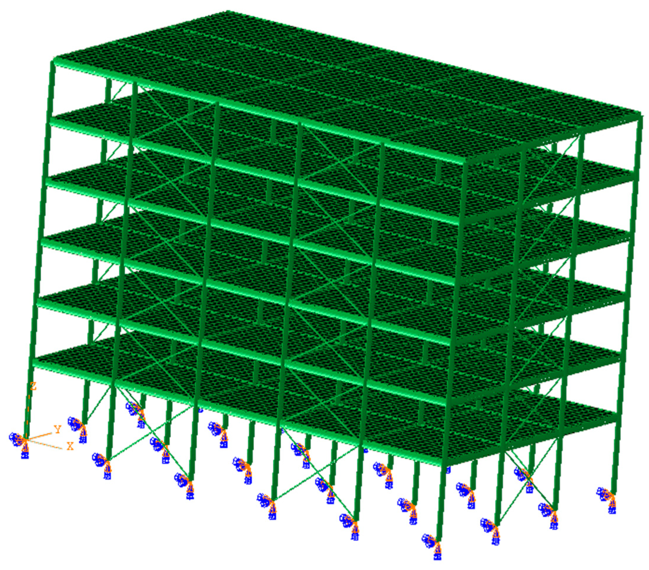
The example structure, which is examined under seismic loadings, is steel structure of a 6-story building. The finite element model of the structure in SIMULIA Abaqus^® v6.14 (2014) is given in Figure 3. It consists of 3792 beam elements, 72 truss elements, and 12,960 shell elements or totally 16,824 elements, 22,062 nodes, and 86,868 variables or $N_{DoF}$.

The structure has 6 columns in X-direction and 4 columns in Y-direction or totally 24 columns of standard steel profile HE 500A [33]. The strong axis of column profiles is oriented in X-direction. All girders are standard steel profile IPE 450 [33]. The girders have their strong axis in Y-direction, if they have their longitudinal axis in X-direction and vise verses. The structure is braced by truss elements corresponding to standard steel profile UPN 120 [33]. The geometric characteristics of profiles, necessary for their finite element section descriptions are given in

Table 2. Geometrical characteristics of standard profiles for the element sections.

Profile	$\mathit{A} \left(\mathbf{c}{\mathbf{m}}^2\right)$	${\mathit{I}}_{\mathit{y}} \left(\mathbf{c}{\mathbf{m}}^4\right)$	${\mathit{I}}_{\mathit{z}} \left(\mathbf{c}{\mathbf{m}}^4\right)$	$\mathit{J} \left(\mathbf{c}{\mathbf{m}}^4\right)$
HE 500A	197.5	86,970	10,370	317.84
IPE 450	98.8	33,740	1676	66.75
UPN 120	17.0	–	–	–

. The elastic modulus of steel is $E=210 \mathrm{G}\mathrm{P}\mathrm{a}$, Poisson’s ratio is $\nu =0.3$, and material density is $\rho =7.85 \mathrm{t}/{\mathrm{m}}^3$.

The floor plates are modeled by shell elements having thickness of 20 cm, Young’s modulus $E=50 \mathrm{G}\mathrm{P}\mathrm{a}$, Poisson’s ratio $\nu =0.2$, and density $\rho =2.5 \mathrm{t}/{\mathrm{m}}^3$, which is close to a homogenized reinforced concrete plate. All elements have a preferable discretization size of 0.5 m and shell elements, and beam elements have common nodes. The distance between the columns is 6 m in both directions, the height of the first story is 4.5 m, and the distance between stories is 3.5 m. The structure is 30 m long in X-direction, 18 m wide in Y-direction, and 22 m high in Z-direction. All columns are fixed in their base.

4. Results and Discussion

The numerical examples using different methods of analysis are run on a work station computer having two processors Intel Xeon E5-1660 v4 @ 3.20 GHz, with eight cores each, but all solutions required eight cores for the calculations. The natural frequency and mode shape analysis shows close first and second frequencies and that the first five modes are enough to satisfy the requirement for the effective modal mass participation, as can be seen in

Table 3. Mode frequencies and mode effective masses.

Mode No.	Frequency, (Hz)	Effec. Mass in X, (t)	Effec. Mass in Y, (t)
1	1.2459	1576.8	0
2	1.3647	0	1547.6
3	1.875	0	0 1
4	3.7649	179.28	0
5	4.2729	0	182.51
Accumulated mass	–	96.77%	95.34%
Residual modes in X and Y, respectively	6.711; 8.1311	48.1	67.2

¹ This mode is twist mode.

, because the structure mass is calculated as 1814.7 tons.

The effects of all seismic loading analyses that are observed, are as follows: the total reaction at the base of columns in the direction of seismic loading, $R_{tot}$; maximum displacement, $d_{max}$; maximum von Misses stress in columns, ${\sigma }_{col}$; maximum von Misses stress in girders, ${\sigma }_{gir}$; and maximum von Misses stress in diagonal bars (truss elements), ${\sigma }_{bar}$. The effects of seismic loadings to the plates are small, so they are ignored here. The total reaction could not be calculated for modal response spectrum method. The results for the modal response spectrum method, are given in

Table 4. Modal response spectrum analysis results.

Loading Direction	Residual Mode	Method	${\mathit{d}}_{\mathit{m}\mathit{a}\mathit{x}}$, (cm)	${\mathit{\sigma }}_{\mathit{c}\mathit{o}\mathit{l}}$, (MPa)	${\mathit{\sigma }}_{\mathit{g}\mathit{i}\mathit{r}}$, (MPa)	${\mathit{\sigma }}_{\mathit{b}\mathit{a}\mathit{r}}$, (MPa)
X	No	CQC	6.662	206.0	85.96	369.2
	Yes	CQC	6.662	206.0	85.97	369.5
	No	SRSS	6.662	206.0	85.96	369.2
	Yes	SRSS	6.662	206.0	85.97	369.5
Y	No	CQC	6.067	196.3	175.6	281.3
	Yes	CQC	6.067	196.4	175.6	281.4
	No	SRSS	6.067	196.3	175.6	281.3
	Yes	SRSS	6.067	196.4	175.6	281.4

.

The results show that there is almost no difference between model with only five modes and the model with five modes plus the residual mode. The difference between methods of gathering the effects of different modes is nothing, although according to EC8 when the one frequency is higher than 90% of the next frequency, the CQC method should be applied, instead of the SRSS method, because they are very close frequencies, and the SRSS method is not appropriate.

Applying the lateral force method, the story masses are assumed to be equal, which means they are ignored in (10) and (11). The base total shear force is calculated for X-direction by the first mode natural frequency, 1.2459 Hz, and this results in $F_{bX}=4878$ kN, while in the Y-direction, using the second natural frequency, 1.3647 Hz, the base shear force is $F_{bY}=5343$ kN.

The results for the lateral force method are given in

Table 5. Lateral force method results.

Loading Direction	Distributions	${\mathit{R}}_{\mathit{t}\mathit{o}\mathit{t}}$, (kN)	${\mathit{d}}_{\mathit{m}\mathit{a}\mathit{x}}$, (cm)	${\mathit{\sigma }}_{\mathit{c}\mathit{o}\mathit{l}}$, (MPa)	${\mathit{\sigma }}_{\mathit{g}\mathit{i}\mathit{r}}$, (MPa)	${\mathit{\sigma }}_{\mathit{b}\mathit{a}\mathit{r}}$, (MPa)
X	Height	4878	6.730	203.0	84.73	357.1
	Mode 1	4878	6.528	200.8	83.74	357.2
Y	Height	5343	6.180	196.5	174.3	278.5
	Mode 1	5343	6.057	195.2	174.2	278.7

. The difference between the ways of distribution of the total base shear force over the stories is comparatively small. There is a difference between the modal response spectrum solution and the lateral force method. The difference, however, is not more than 4%, and it is higher when the loading is in the X-direction, in which direction the structure is stiffer.

The time history simulations of seismic loading by accelerograms should be completed in the same conditions as response spectrum methods, which means with the same damping ratio $\zeta =5$%. In order to do that, damping by Rayleigh is assumed, which is determined by the formula:

$$\zeta ={\displaystyle \frac{\alpha }{2{\omega }_1 }}+{\displaystyle \frac{\beta {\omega }_1}{2}}$$

(22)

where ${\omega }_1=2\pi f_1$ is the fundamental angular frequency of the structure and it is assumed that $\beta =0$. The obtained value for $\alpha$ is $\alpha =0.78282$.

The simulations are run for a 40 s problem time and 2000 states are recorded. The implicit method of simulations as well as the modal dynamics method have 8000 increments with fixed time step, while the explicit method has 2,143,928 increments. The wall-clock time for running the time history analysis using different accelerograms is given in

Table 6. Wall-clock time for running time history analysis.

Direction	Accelerogram No	Explicit, (s)	Implicit, (s)	Modal, 5 m, (s)	Modal, 6 m, (s)
	1	6118	5307	1096	1137
X	2	6146	5186	1075	1100
	3	6326	5283	1087	1166
	1	6240	5148	1137	1120
Y	2	6290	5259	1088	1082
	3	6293	5242	1081	1076

in seconds.

The fastest analysis is the modal dynamics analysis, which has approximately 18 min for running, but this method is linear elastic by origin. The explicit analysis is running for approximately 1 h and 40 min, which is quite longer, but the method can be totally nonlinear, because it is on the level of sound wave tracking. The implicit time history analysis has time for running approximately 1 h and 25 min. This is not very different than explicit simulations, because the building frame structures are very simple with relatively few DOF and high critical time step, where the explicit analysis has better performance, although it runs in double precision calculations.

The results for the effects of seismic loading for the different time history analyses are given in

Table 7. Time history analysis by artificial accelerograms.

Loading Direction	Method	Accelerogram No	${\mathit{R}}_{\mathit{t}\mathit{o}\mathit{t}}$, (kN)	${\mathit{d}}_{\mathit{m}\mathit{a}\mathit{x}}$, (cm)	${\mathit{\sigma }}_{\mathit{c}\mathit{o}\mathit{l}}$, (MPa)	${\mathit{\sigma }}_{\mathit{g}\mathit{i}\mathit{r}}$, (MPa)	${\mathit{\sigma }}_{\mathit{b}\mathit{a}\mathit{r}}$, (MPa)
X		1	4821	6.374	195.3	82.12	353.5
	Explicit	2	5199	6.770	212.1	87.45	382.0
		3	4811	6.726	193.2	87.14	351.4
		1	4830	6.381	197.3	82.49	354.5
	Implicit	2	5212	6.783	210.7	87.82	383.1
		3	4814	6.735	192.3	87.17	352.1
		1	4898	6.369	197.1	82.37	358.4
	Modal, 5 modes	2	5254	6.766	209.1	87.36	384.5
		3	4762	6.748	191.4	85.39	348.5
		1	5666	6.377	216.9	89.16	407.5
	Modal, 6 modes	2	5 533	6.718	215.3	90.68	402.3
		3	5033	6.711	197.0	87.17	365.8
Y		1	5186	5.637	180.1	163.0	267.9
	Explicit	2	6095	6.523	215.7	193.8	314.3
		3	5762	6.323	202.3	182.5	298.3
		1	5175	5.658	180.1	163.8	267.6
	Implicit	2	6338	6.539	221.4	199.0	326.0
		3	5826	6.382	203.7	185.1	300.4
		1	5199	5.657	183.3	165.1	268.8
	Modal, 5 modes	2	6130	6.575	217.8	196.6	317.7
		3	5881	6.363	205.5	186.8	304.3
		1	5284	5.650	182.2	165.1	271.6
	Modal, 6 modes	2	6117	6.575	217.6	196.5	317.3
		3	5899	6.350	204.4	186.4	302.3

. The first expression is that there is a quite different response to the different accelerograms. Another issue is that the implicit and the modal transient simulations show a little bit higher value, compared with the explicit analysis and the values of modal dynamics method with six modes (five modes + residual mode) in X-direction are significantly higher.

The effects of the accelerogram No.2 simulations are highest and let compare them to the other two accelerogram response. Taking as a reference the second accelerogram effects the relative divergency for explicit analysis is calculated and shown in

Table 8. Relative divergency of accelerogram effects for explicit compared to accelerogram No.2.

Loading Direction	Accelerogram No.	${\mathit{R}}_{\mathit{t}\mathit{o}\mathit{t}}$, %	${\mathit{d}}_{\mathit{m}\mathit{a}\mathit{x}}$, %	${\mathit{\sigma }}_{\mathit{c}\mathit{o}\mathit{l}}$, %	${\mathit{\sigma }}_{\mathit{g}\mathit{i}\mathit{r}}$, %	${\mathit{\sigma }}_{\mathit{b}\mathit{a}\mathit{r}}$, %
X	1	7.27	5.85	7.92	6.09	7.46
	3	7.46	0.65	8.91	0.35	8.01
Y	1	14.91	13.58	16.50	15.89	14.76
	3	5.46	3.07	6.21	5.83	5.09

. The relative divergency is calculated in percent by formula:

$$relative divergency={\displaystyle \frac{reference value-relative value}{reference value }} 100\%$$

(23)

The results in Table 8 show a comparatively great divergency of the dynamic response of the structure to the accelerograms. The greatest one is 16.5%. Let us compare the different methods for time history analysis to the explicit method by calculating the relative divergency only for an accelerogram No.2. The results are given in

Table 9. Relative divergency of effects for time history analysis compared to explicit method by accelerogram No.2.

Loading Direction	Method	${\mathit{R}}_{\mathit{t}\mathit{o}\mathit{t}}$, %	${\mathit{d}}_{\mathit{m}\mathit{a}\mathit{x}}$, %	${\mathit{\sigma }}_{\mathit{c}\mathit{o}\mathit{l}}$, %	${\mathit{\sigma }}_{\mathit{g}\mathit{i}\mathit{r}}$, %	${\mathit{\sigma }}_{\mathit{b}\mathit{a}\mathit{r}}$, %
	Implicit	−0.25	−0.19	0.66	−0.42	−0.29
X	Modal, 5 modes	−1.06	0.06	1.41	0.10	−0.65
	Modal, 6 modes	−6.42	0.77	−1.51	−3.69	−5.31
	Implicit	−3.99	−0.25	−2.64	−2.68	−3.72
Y	Modal, 5 modes	−0.57	−0.80	−0.97	−1.44	−1.08
	Modal, 6 modes	−0.36	−0.80	−0.88	−1.39	−0.95

.

The results in Table 9 show that all methods for time history analysis have a comparatively close assessment of the effects of seismic loadings. The positive divergency is a maximum 1.4% and a negative divergency means overestimated values, in which the maximum is 6.4%, but it is on the side of safety.

From a safety point of view, the highest dynamic response of the structure to the accelerograms should be taken as a basis for design. The assessment of effectiveness of the response spectrum method is completed by calculating the relative divergency of the effects of seismic loading compared to explicit analysis using accelerogram No.2. The results are given in

Table 10. Relative divergency of effects for response spectrum methods compared to explicit method, accelerogram No.2.

Loading Direction	Method	${\mathit{d}}_{\mathit{m}\mathit{a}\mathit{x}}$, %	${\mathit{\sigma }}_{\mathit{c}\mathit{o}\mathit{l}}$, %	${\mathit{\sigma }}_{\mathit{g}\mathit{i}\mathit{r}}$, %	${\mathit{\sigma }}_{\mathit{b}\mathit{a}\mathit{r}}$
	Modal response spectrum	1.60	2.88	1.70	3.35
X	Lateral force., height distr.	0.59	4.29	3.11	6.52
	Lateral force., mode 1 distr.	3.57	5.33	4.24	6.49
	Modal response spectrum	6.99	8.95	9.39	10.47
Y	Lateral force., height distr.	5.26	8.90	10.06	11.39
	Lateral force., mode 1 distr.	7.14	9.50	10.11	11.33

.

The analysis of data in Table 10 shows that the response spectrum methods can give us approximately 10% underestimation of seismic effects to the structure and especially to the weak direction of the structure. The modal response spectrum method can run for a few seconds, but it is not as conservative as it is believed. The structure should be examined even with more artificial accelerograms in order to find the maximum response and to reveal its behavior.

5. Conclusions

The different representations of seismic loading show some differences in the effects of that loading. Although the artificial accelerograms are pointed out as an alternative representation of seismic loadings to the response spectrum, they could become an essential part of the analysis for seismic resistance of building structures in the stage of their design. The following conclusions can be drawn:

• The artificial accelerograms, although having very similar spectra, have a great diversity in the dynamic response of structures and in the effects of loadings. Looking for the maximum response and effects, it is necessary to try more than the minimum requirement of three accelerograms in one direction.
• All methods for time history analysis have similar results, and the fastest and cheapest method is the modal transient dynamic method, which, however, is the only linear method of analysis. The method could reveal torsional effects and structural response with higher stresses.
• When nonlinear simulations with accelerograms are needed, the explicit time integration method is superior and it is not so expensive, because the building frame structure model have relatively few DOF and a high critical time step, so it can be easily calculated even with a double precision, while the implicit nonlinear method could have low convergence and slower calculation.
• The response spectrum methods are very fast and easy for calculations. However, they are not so conservative. Compared with time history analysis methods, they can underestimate the effects of seismic loadings by approximately 10%, but use more diverse accelerograms, and the underestimation could be even greater.

References

- EN 1998-1; Eurocode 8: Design of Structures for Earthquake Resistance—Part 1: General Rules, Seismic Actions and Rules for Buildings. European Committee for Standardization: Brussels, Belgium, 2004; pp. 33–76.
- Chopra, A.K. Dynamics of Structures: Theory and Applications to Earthquake Engineering, 4th ed.; Prentice-Hall of India: New Delhi, India, 2005. [Google Scholar]
- Gupta, A.K.; Hall, W.J. Response Spectrum Method: In Seismic Analysis and Design of Structures; CRC Press: Boca Raton, FL, USA, 2017. [Google Scholar]
- Hadjian, A.H. Seismic response of structures by the response spectrum method. Nucl. Eng. Des. 1981, 66, 179–201. [Google Scholar] [CrossRef]
- Gupta, A.K.; Chen, D.C. Comparison of modal combination methods. Nucl. Eng. Des. 1984, 78, 53–68. [Google Scholar] [CrossRef]
- Khatiwada, P.; Hu, Y.; Lumantarna, E.; Menegon, S.J. Dynamic Modal Analyses of Building Structures Employing Site-Specific Response Spectra Versus Code Response Spectrum Models. CivilEng 2023, 4, 134–150. [Google Scholar] [CrossRef]
- Dhileep, M.; Bose, P.R. A comparative study of “missing mass” correction methods for response spectrum method of seismic analysis. Comp. Struct. 2008, 86, 2087–2094. [Google Scholar] [CrossRef]
- Salmonte, A.J. Considerations on the residual contribution in modal analysis. Earthq. Eng. Struc. Dyn. 1982, 10, 295–304. [Google Scholar] [CrossRef]
- Fragiadakis, M.; Papadrakakis, M. Modeling, analysis and reliability of seismically excited structures: Computational issues. Int. J. Comput. Methods 2008, 5, 483–511. [Google Scholar] [CrossRef]
- Argyris, J.H.; Hilpert, O.; Malejannakis, G.A.; Scharpf, D.W. On the geometrical stiffness of a beam in space—A consistent v. w. approach. Comput. Meth. Appl. Mech. Eng. 1979, 20, 105–131. [Google Scholar] [CrossRef]
- Filippou, F.C.; Fenves, G.L. Ch. 6 Methods of analysis for earthquake-resistant structures. In Earthquake Engineering: From Engineering Seismology to Performance-Based Engineering; CRC Press: Boca Raton, FL, USA, 2004; eBook; ISBN 9780429204968. [Google Scholar]
- Fajfar, P.; Gaspersic, P. The N2 method for the seismic damage analysis of RC buildings. Earthq. Eng. Struct. Dyn. 1996, 25, 31–46. [Google Scholar] [CrossRef]
- Krawinkler, H.; Seneviratna, G.D.P.K. Pros and cons of a pushover analysis of seismic performance evaluation. Eng. Struct. 1998, 20, 452–464. [Google Scholar] [CrossRef]
- Chopra, A.K.; Goel, R.K. A modal pushover analysis procedure for estimating seismic demands for buildings. Earthq. Eng. Struct. Dyn. 2002, 31, 561–582. [Google Scholar] [CrossRef]
- Aschheima, M.; Tjhinb, T.; Comartinc, C.; Hamburgerd, R.; Inele, M. The scaled nonlinear dynamic procedure. Eng. Struct. 2007, 29, 1422–1441. [Google Scholar] [CrossRef]
- Li, H.; Du, Y.; Han, J.; Li, F. Investigation on seismic behavior of a new beam-column joint for precast concrete structures under reversed cyclic loading. Structures 2024, 70, 107782. [Google Scholar] [CrossRef]
- Foti, F.; Lago, B.D.; Martinelli, L. On the coupled dynamics of vertical cladding panels and industrial frame structures subject to out-of-plane seismic loading. Eng. Struct. 2023, 296, 116909. [Google Scholar] [CrossRef]
- Jayaram, N.; Lin, T.; Baker, J.W. A computationally efficient ground-motion selection algorithm for matching a target response spectrum mean and variance. Earthq. Spectra 2011, 27, 797–815. [Google Scholar] [CrossRef]
- Baker, J.W.; Cornell, C. Spectral shape, epsilon and record selection. Earthq. Eng. Struct. Dyn. 2006, 35, 1077–1095. [Google Scholar] [CrossRef]
- Iervolino, I.; De Luca, F.; Cosenza, E. Spectral shape-based assessment of SDOF nonlinear response to real, adjusted and artificial accelerograms. Eng. Struct. 2010, 32, 2776–2792. [Google Scholar] [CrossRef]
- Baker, J.W. Conditional mean spectrum: Tool for ground-motion selection. J. Struct. Eng. 2011, 137, 322–331. [Google Scholar] [CrossRef]
- Hu, Y.; Lam, N.; Menegon, S.J.; Wilson, J. The Selection and Scaling of Ground Motion Accelerograms for Use in Stable Continental Regions. J. Earthq. Eng. 2022, 26, 6284–6303. [Google Scholar] [CrossRef]
- Lam, N.; Wilson, J.; Hutchinson, G. Generation of synthetic earthquake accelerograms using seismological modelling: A review. J. Earthq. Eng. 2000, 4, 321–354. [Google Scholar] [CrossRef]
- Suárez, L.E.; Montejo, L.A. Generation of artificial earthquakes via the wavelet transform. Int. J. Solids Struct. 2005, 42, 5905–5919. [Google Scholar] [CrossRef]
- Causse, M.; Laurendeau, A.; Perrault, M.; Douglas, J.; Bonilla, L.F.; Guéguen, P. Eurocode 8-compatible synthetic time-series as input to dynamic analysis. Bullet. Earthq. Eng. 2014, 12, 755–768. [Google Scholar] [CrossRef]
- Trovato, S.; D’Amore, E.; Yue, Q.; Spanos, P.D. An approach for synthesizing tri-component ground motions compatible with hazard-consistent target spectrum—Italian aseismic code application. Soil Dyn. Earthq. Eng. 2017, 93, 121–134. [Google Scholar] [CrossRef]
- Wu, S.R.; Gu, L. Introduction to the Explicit Finite Element Method for Nonlinear Transient Dynamics; John Wiley & Sons, Inc.: Hoboken, NJ, USA, 2012. [Google Scholar]
- Belytschko, T.; Liu, W.K.; Moran, B. Nonlinear Finite Elements in for Continua and Structures; John Wiley & Sons: Chichester, UK, 2000. [Google Scholar]
- Petyt, M. Introduction to Finite Element Vibration Analysis, 2nd ed.; Cambridge University Press: New York, NY, USA, 2010; pp. 367–412. [Google Scholar]
- Bommer, J.J.; Stafford, P.J. Seismic hazard and earthquake actions. In Seismic Design of Buildings to Eurocode 8, 2nd ed.; Elghazouli, A.Y., Ed.; CRC Press, Taylor & Francis: Boca Raton, FL, USA, 2017; pp. 7–40. [Google Scholar]
- Bathe, K.J.; Cimento, A.P. Some practical procedures for the solution of nonlinear finite element equations. Comput. Meth. Appl. Mech. Eng. 1980, 22, 59–85. [Google Scholar] [CrossRef]
- Ferreira, F.; Moutinho, C.; Cunha, Á.; Caetano, E. An artificial accelerogram generator code written in Matlab. Eng. Rep. 2020, 2, e12129. [Google Scholar] [CrossRef]
- EN 10365; Hot rolled steel channels, I and H sections - Dimensions and masses. European Committee for Standardization: Brussels, Belgium, 2015.
Disclaimer/Publisher’s Note: The statements, opinions and data contained in all publications are solely those of the individual author(s) and contributor(s) and not of MDPI and/or the editor(s). MDPI and/or the editor(s) disclaim responsibility for any injury to people or property resulting from any ideas, methods, instructions or products referred to in the content. |
© 2025 by the authors. Licensee MDPI, Basel, Switzerland. This article is an open access article distributed under the terms and conditions of the Creative Commons Attribution (CC BY) license (https://creativecommons.org/licenses/by/4.0/).