
An Interval Process Method for Non-Random Uncertain Aeroelastic Analysis


Abstract
:1. Introduction and Background
2. Theory
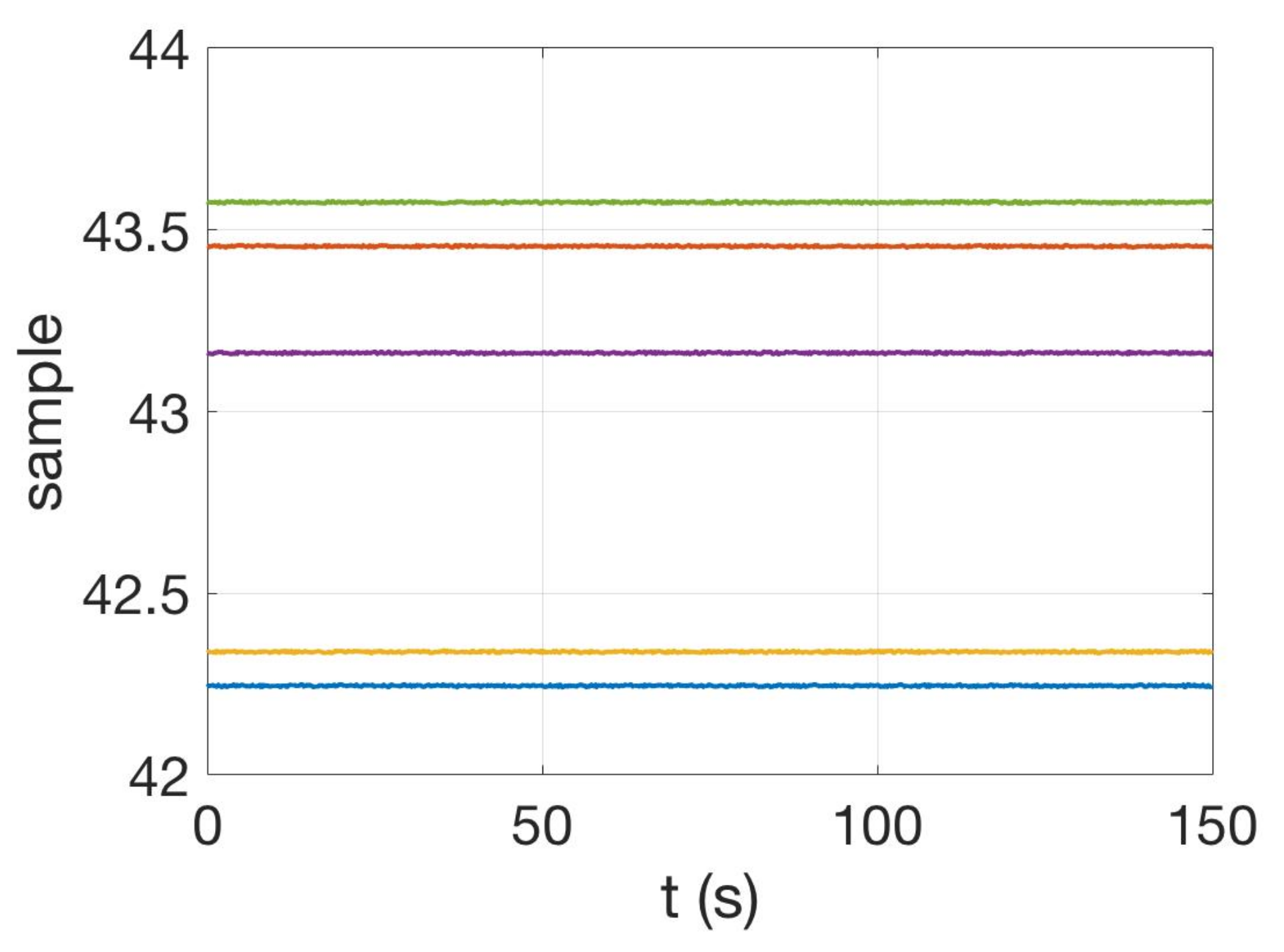
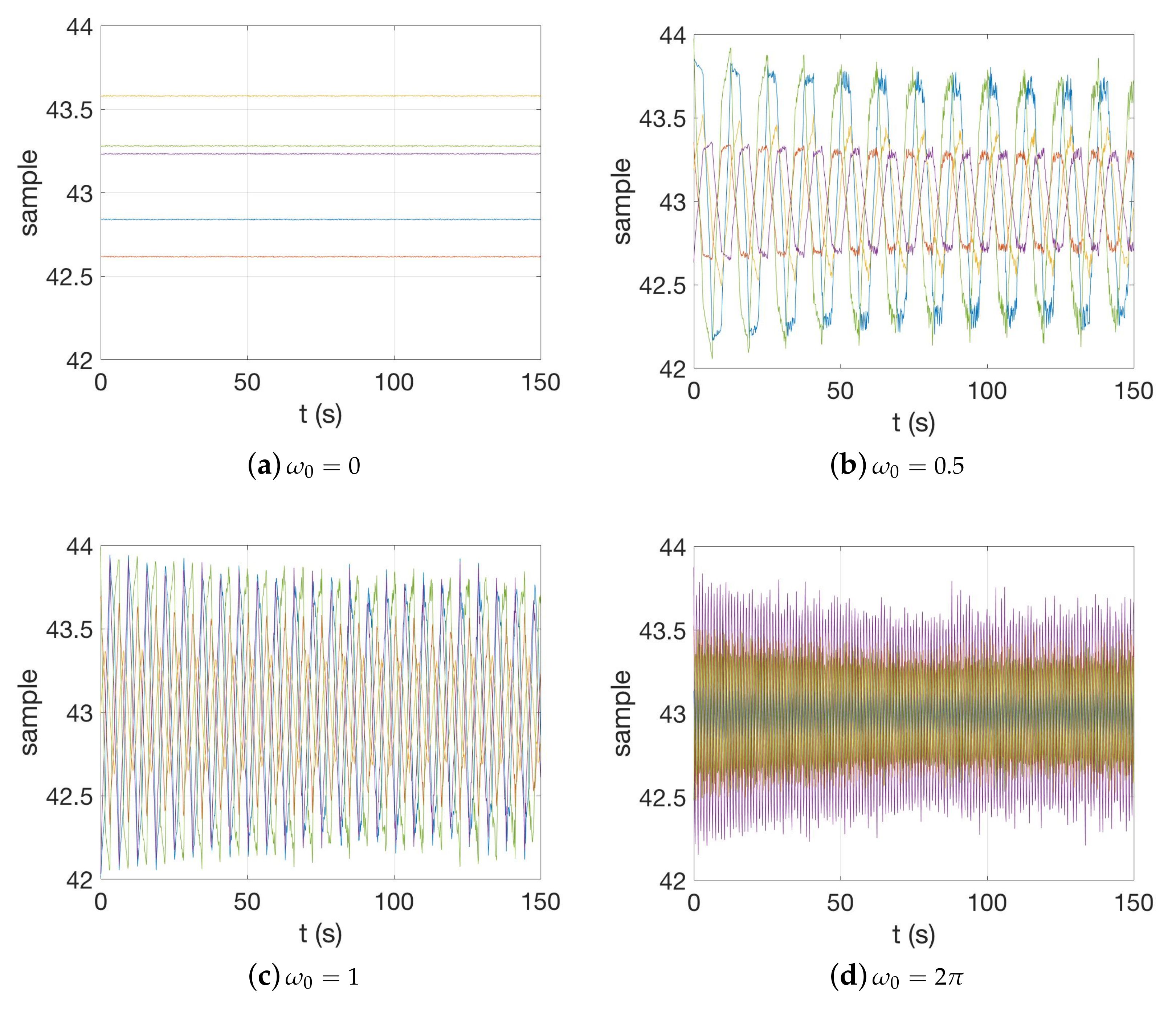
2.1. Sampling
- Step 1:
- Calculate the average and half-width functions from the given upper and lower limits. Then calculate the correlation matrix, , from the given correlation function, .
- Step 2:
- Use the modified Cholesky decomposition [23] to create the lower triangular matrix, , from the correlation matrix, .
- Step 3:
- Generate an auxiliary independent interval process, , such that , for all . This is a sample of uniformly distributed random numbers in , .
- Step 4:
- Using the lower triangular transformation of the correlation matrix, , transform y to , . is a new sample in the interval of with correlation matrix .
- Step 5:
- Finally, use linear translation and stretching transformation on to get the sample in with the correlation matrix.
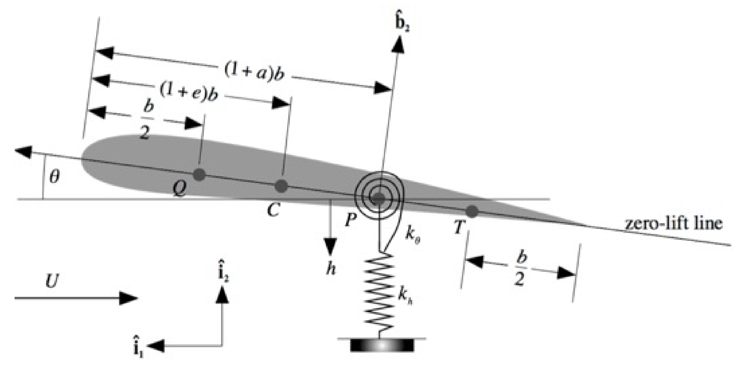
2.2. Deterministic Solver for an Airfoil Cross-Section
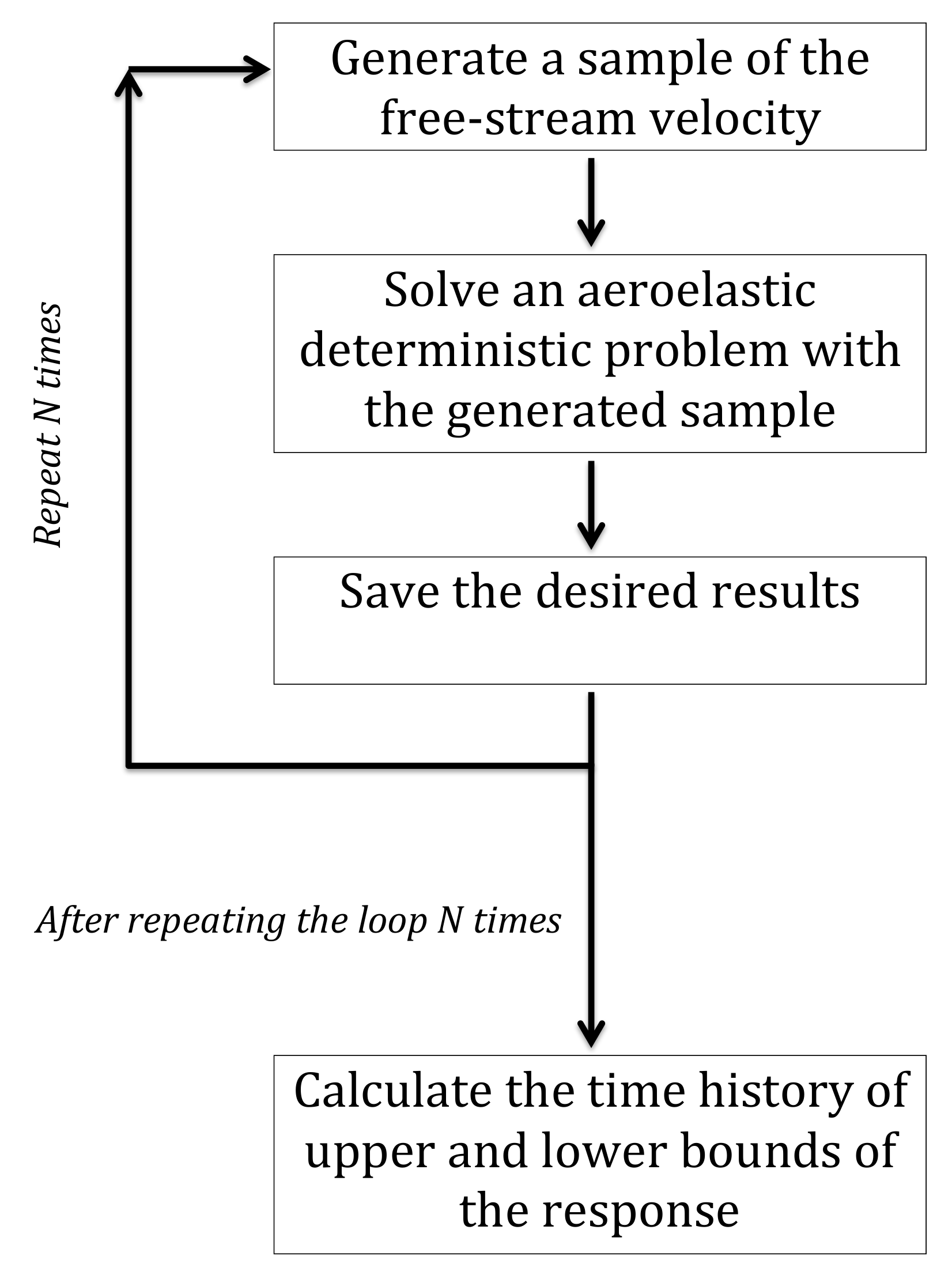
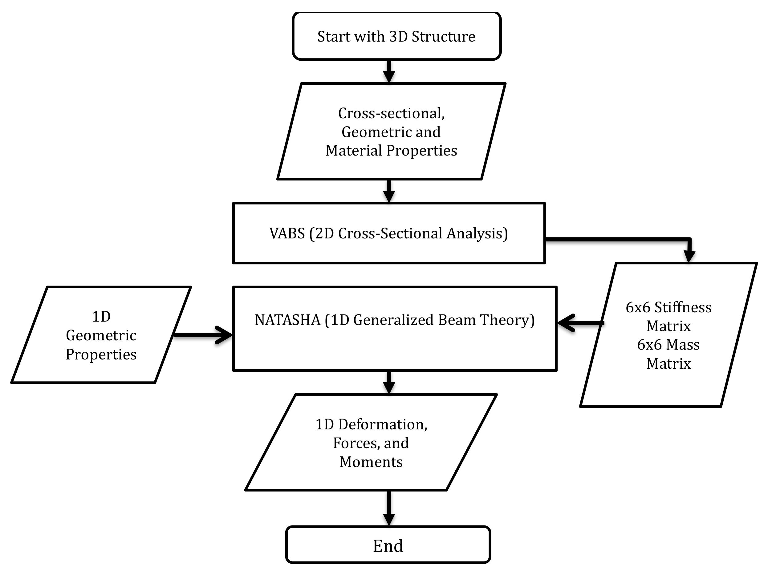
2.3. Deterministic Solver for a High-Aspect Ratio Wing
3. Numerical Results
3.1. Sampling
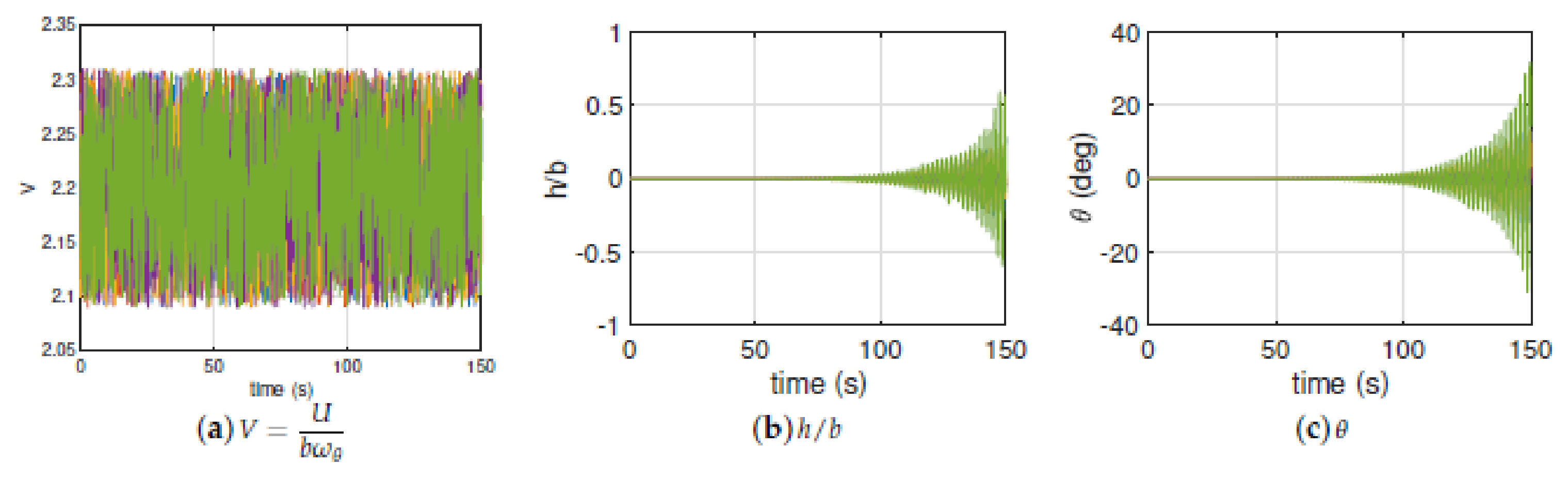
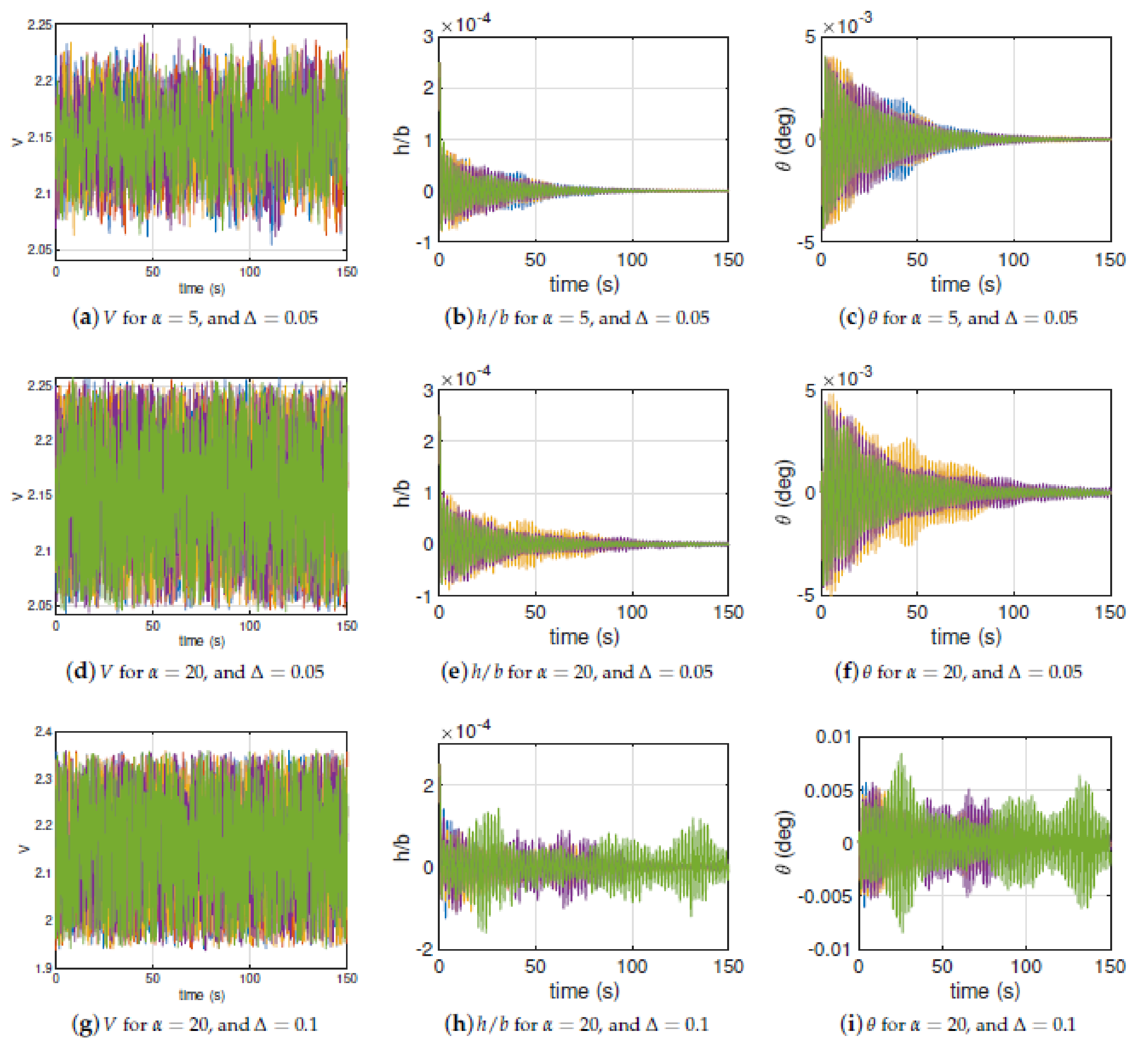
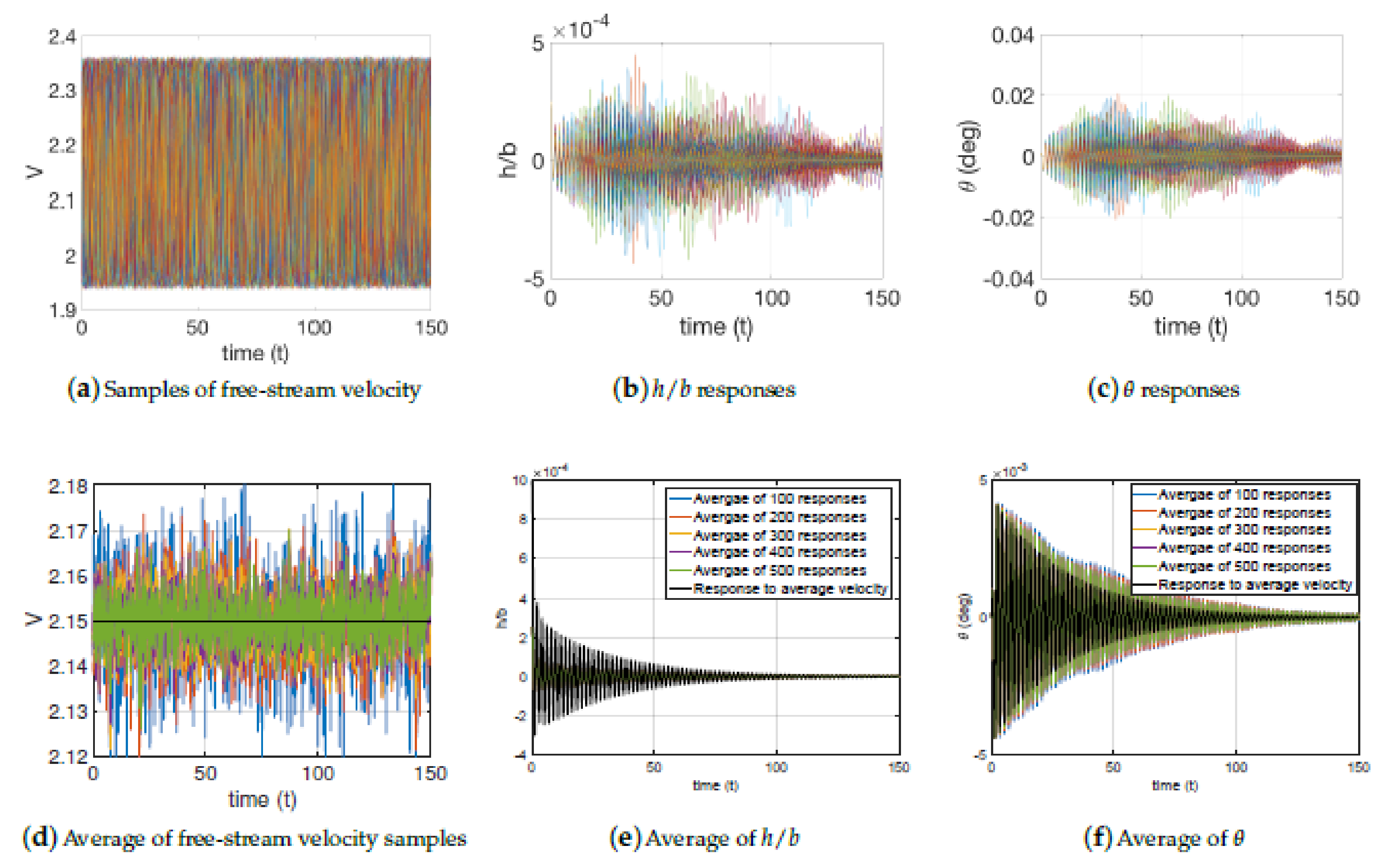
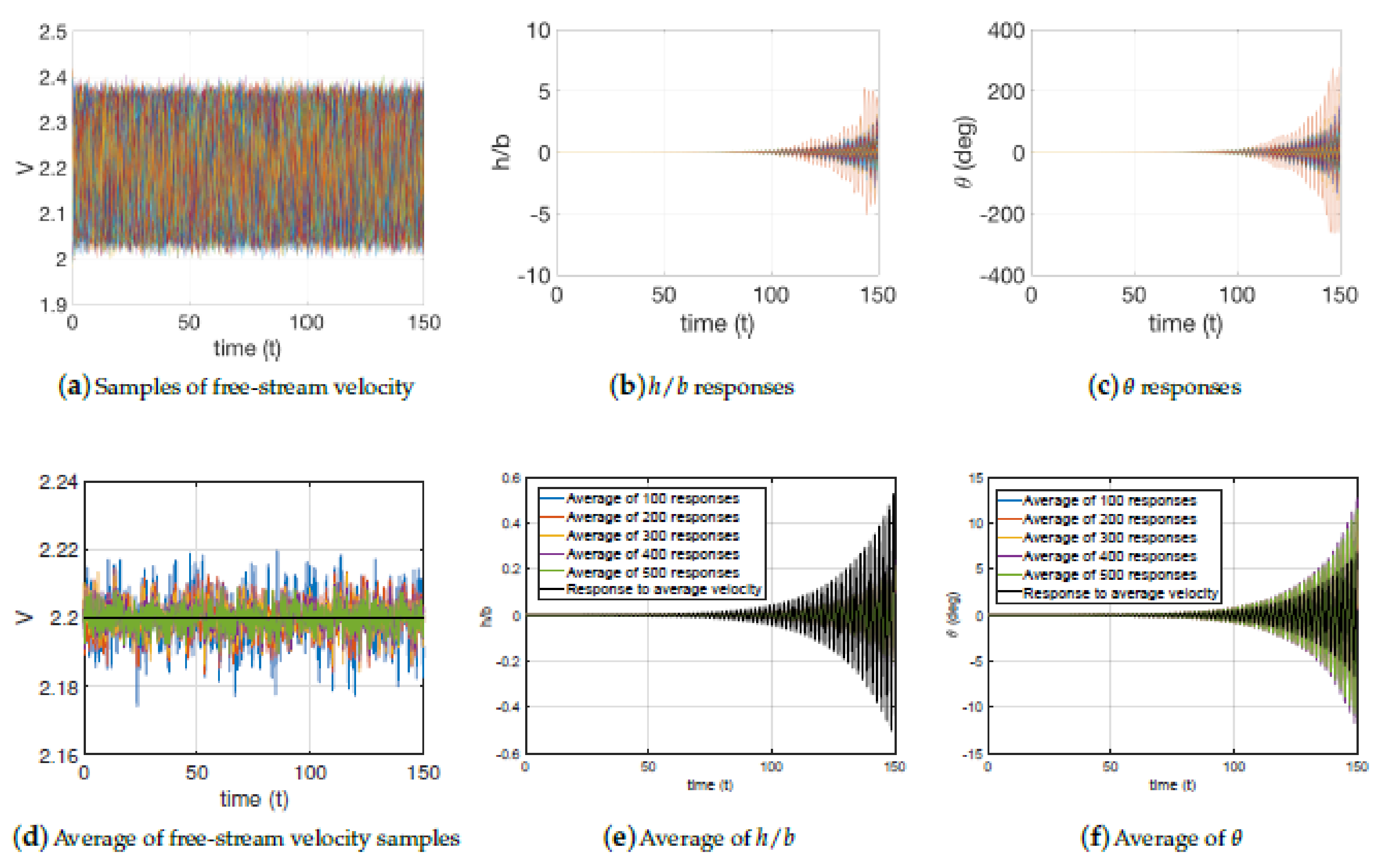
3.2. Airfoil Cross-Section
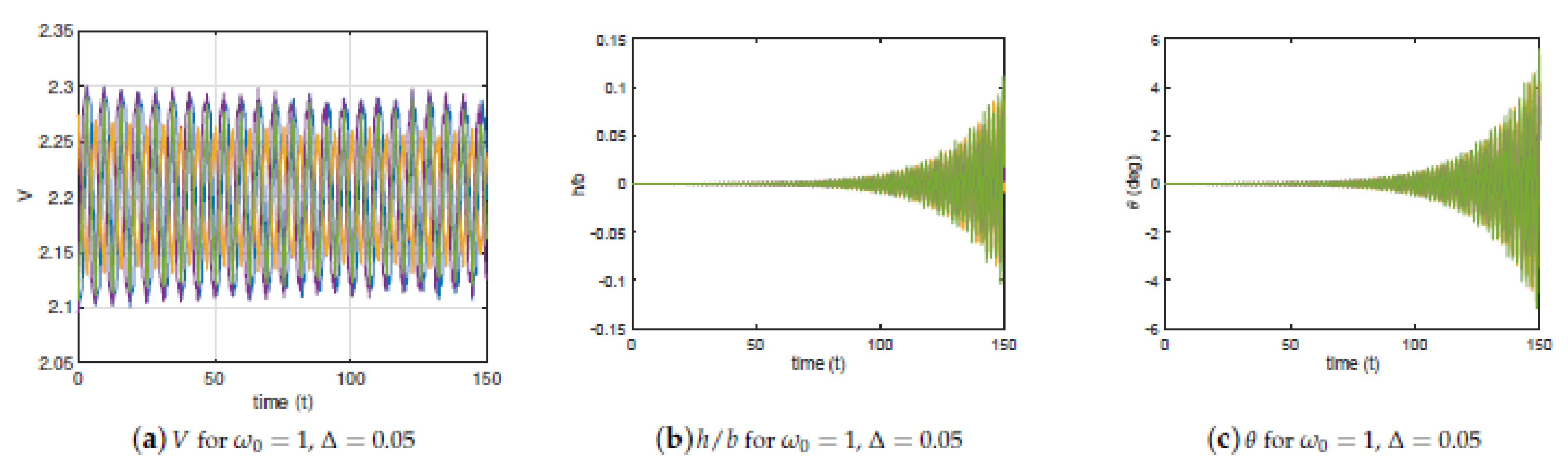
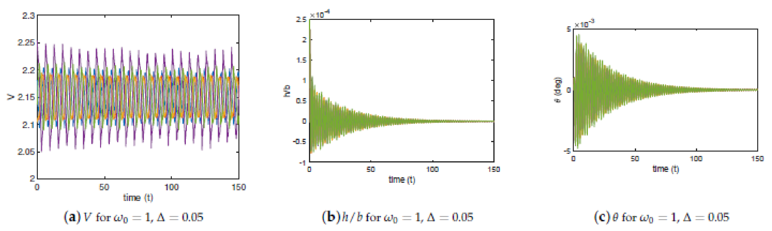
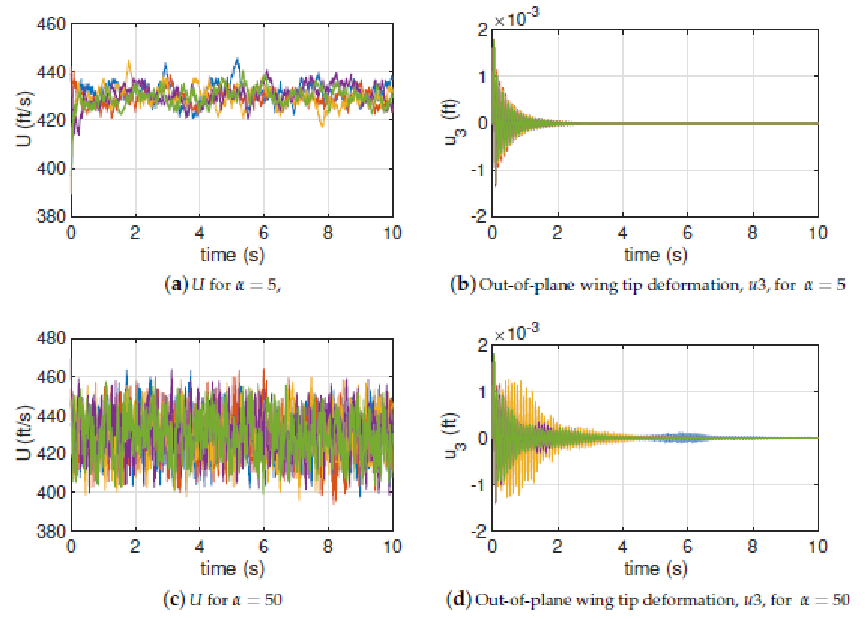
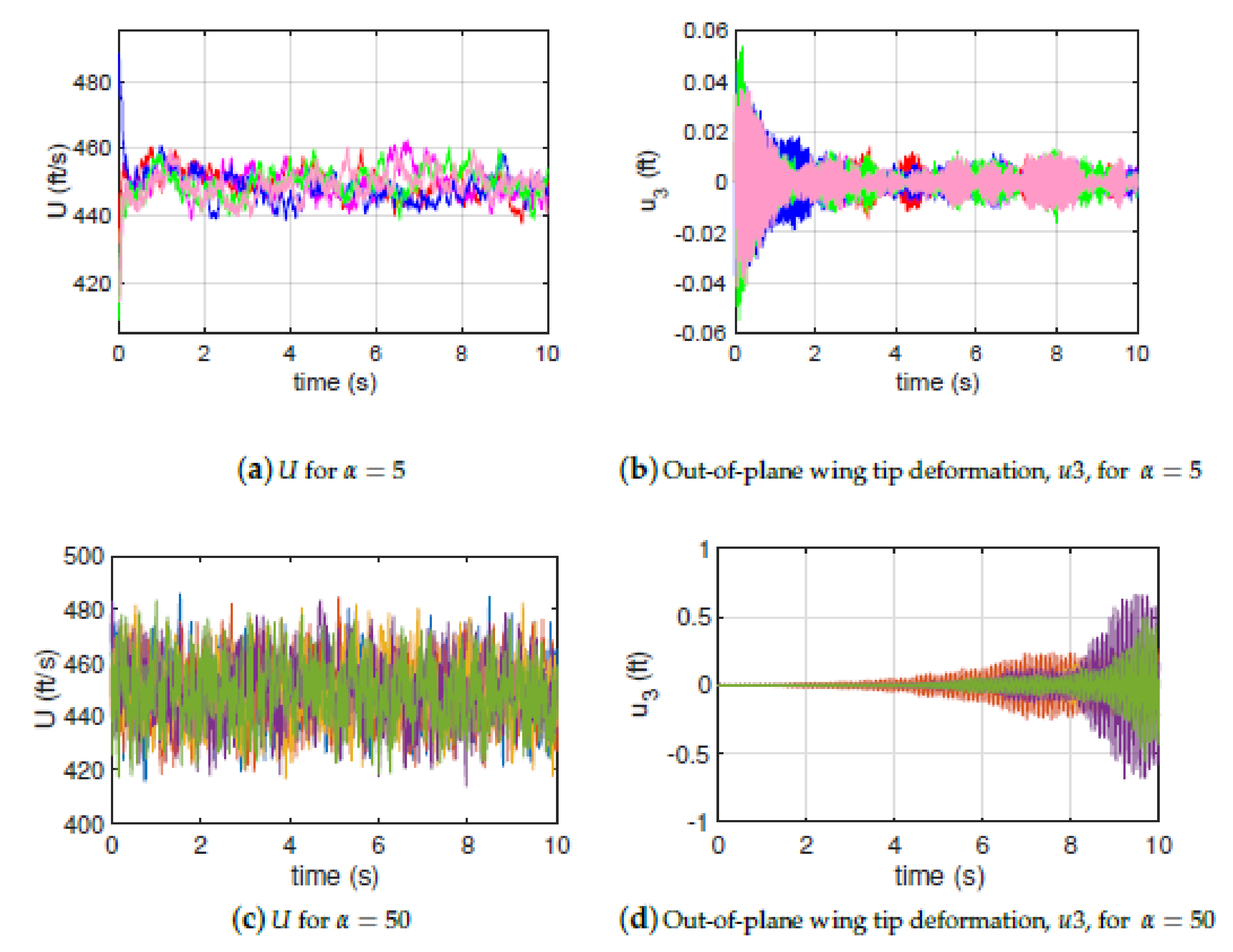
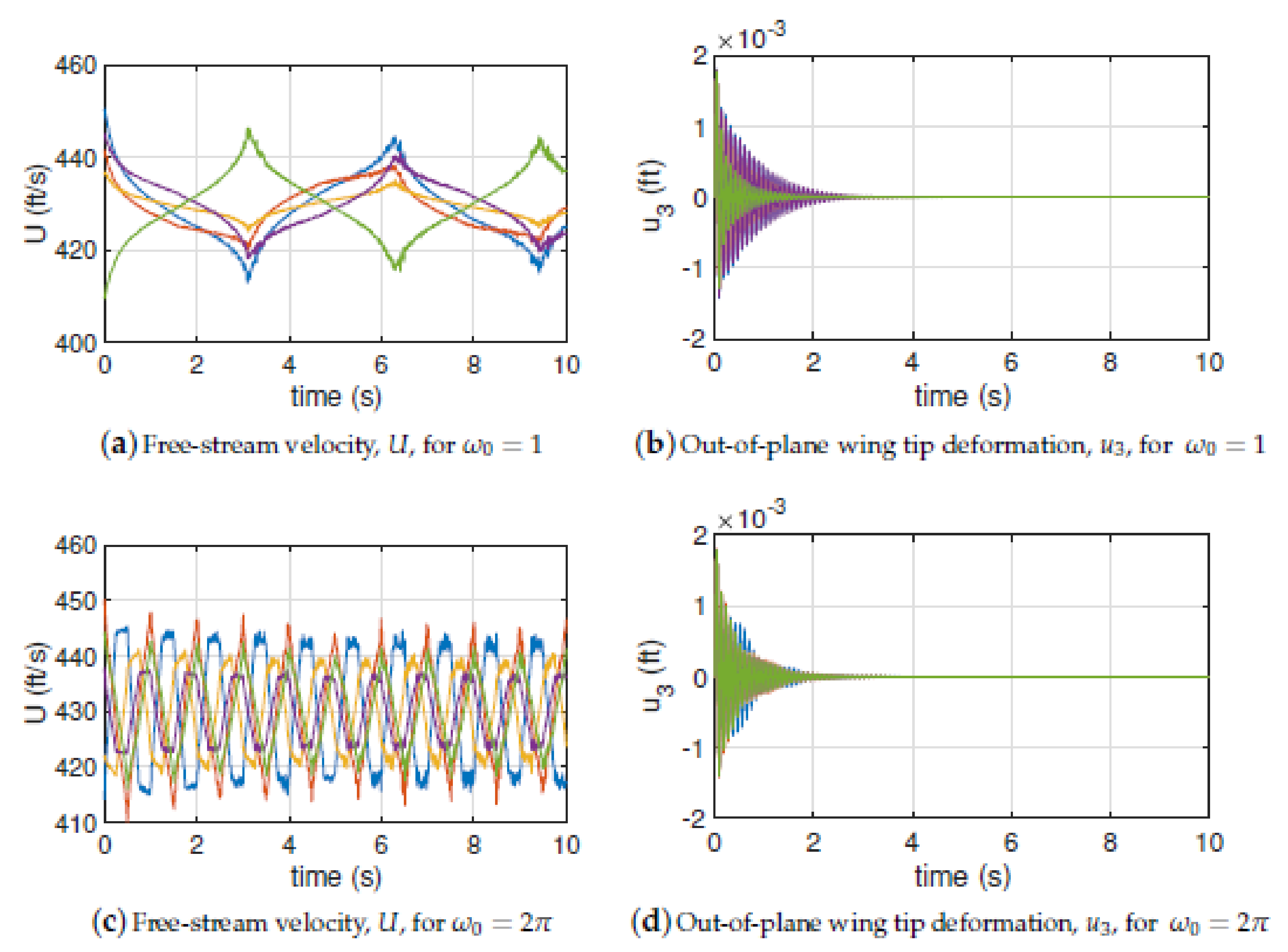
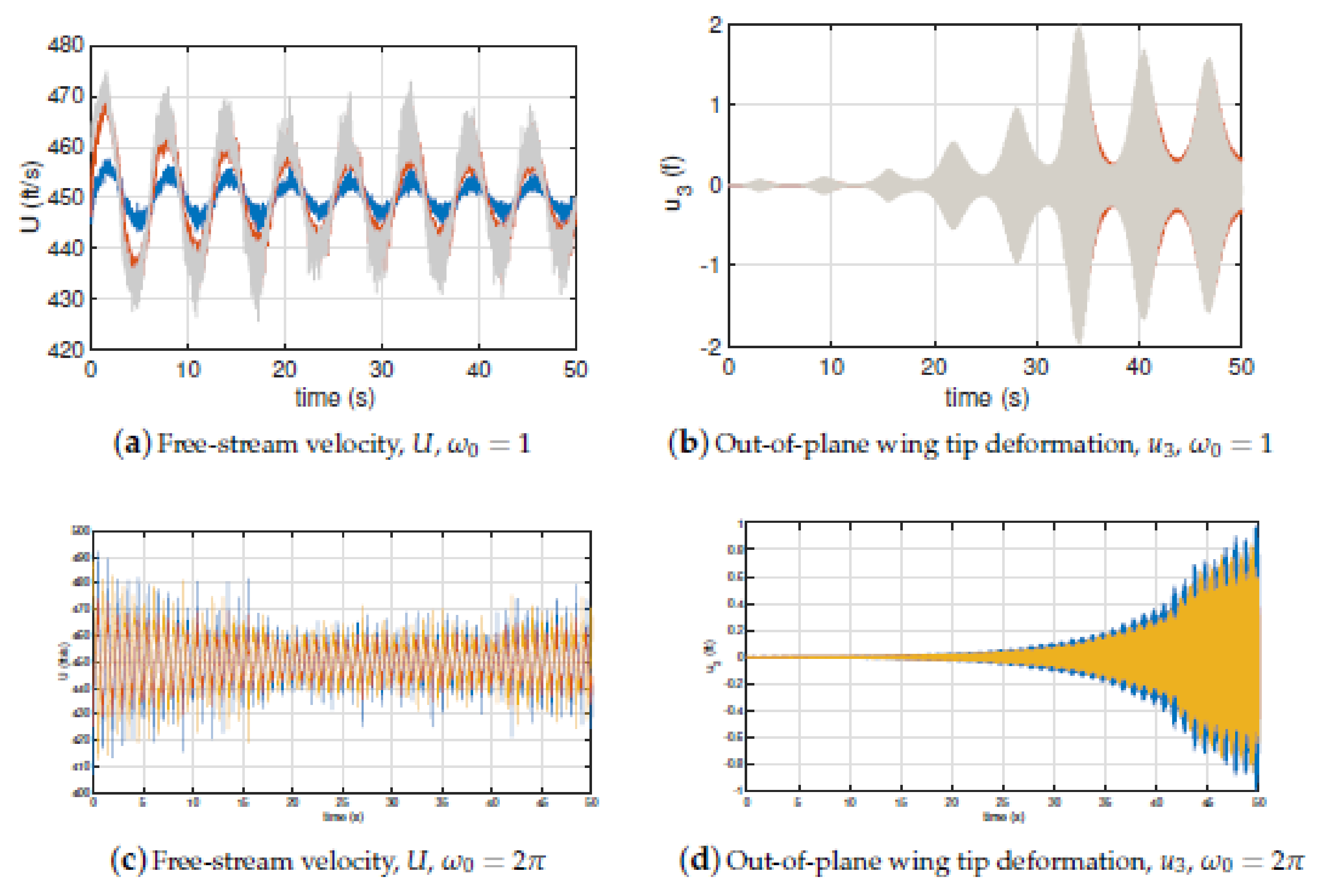
3.3. High-Aspect Ratio Wing
4. Conclusions
Author Contributions
Funding
Data Availability Statement
Conflicts of Interest
References
- Pettit, C.L. Uncertainty Quantification in Aeroelasticity: Recent Results and Research Challenges. J. Aircr. 2004, 41, 1217–1229. [Google Scholar] [CrossRef]
- Riley, M.E.; Grandhi, R.V.; Kolonay, R. Quantification of modeling uncertainty in aeroelastic analyses. J. Aircr. 2011, 48, 866–873. [Google Scholar] [CrossRef]
- Nitschke, C.T.; Cinnella, P.; Lucor, D.; Chassaing, J.C. Model-form and predictive uncertainty quantification in linear aeroelasticity. J. Fluids Struct. 2017, 73, 137–161. [Google Scholar] [CrossRef] [Green Version]
- Chakraverty, S. Mathematics of Uncertainty Modeling in the Analysis of Engineering and Science Problems; IGI Global: Hershey, PA, USA, 2014. [Google Scholar]
- Beran, P.; Stanford, B.; Schrock, C. Uncertainty quantification in aeroelasticity. Annu. Rev. Fluid Mech. 2017, 49, 361–386. [Google Scholar] [CrossRef]
- Georgiou, G.; Manan, A.; Cooper, J. Modeling composite wing aeroelastic behavior with uncertain damage severity and material properties. Mech. Syst. Signal Process. 2012, 32, 32–43. [Google Scholar] [CrossRef]
- Sarma, R.; Dwight, R.P. Uncertainty Reduction in Aeroelastic Systems with Time-Domain Reduced-Order Models. AIAA J. 2017, 55, 2437–2449. [Google Scholar] [CrossRef]
- Tartaruga, I.; Sartor, P.; Cooper, J.E.; Coggon, S.; Lemmens, Y. Efficient prediction and uncertainty propagation of correlated loads. In Proceedings of the 56th AIAA/ASCE/AHS/ASC Structures, Structural Dynamics, and Materials Conference, Kissimmee, FL, USA, 5–9 January 2015; p. 1847. [Google Scholar]
- Attar, P.J.; Dowell, E.H. Stochastic analysis of a nonlinear aeroelastic model using the response surface method. J. Aircr. 2006, 43, 1044–1052. [Google Scholar] [CrossRef]
- Borello, F.; Cestino, E.; Frulla, G. Structural uncertainty effect on classical wing flutter characteristics. J. Aerosp. Eng. 2010, 23, 327–338. [Google Scholar] [CrossRef]
- Sarkar, S.; Witteveen, J.; Loeven, A.; Bijl, H. Effect of uncertainty on the bifurcation behavior of pitching airfoil stall flutter. J. Fluids Struct. 2009, 25, 304–320. [Google Scholar] [CrossRef]
- Desai, A.; Sarkar, S. Analysis of a nonlinear aeroelastic system with parametric uncertainties using polynomial chaos expansion. Math. Probl. Eng. 2010, 2010, 379472. [Google Scholar] [CrossRef]
- Hayes, R.; Marques, S.P. Prediction of limit cycle oscillations under uncertainty using a harmonic balance method. Comput. Struct. 2015, 148, 1–13. [Google Scholar] [CrossRef] [Green Version]
- Lokatt, M. Aeroelastic flutter analysis considering modeling uncertainties. J. Fluids Struct. 2017, 74, 247–262. [Google Scholar] [CrossRef]
- Murugan, S.; Ganguli, R.; Harursampath, D. Aeroelastic response of composite helicopter rotor with random material properties. J. Aircr. 2008, 45, 306–322. [Google Scholar] [CrossRef]
- Khodaparast, H.H.; Mottershead, J.E.; Badcock, K.J. Propagation of structural uncertainty to linear aeroelastic stability. Comput. Struct. 2010, 88, 223–236. [Google Scholar] [CrossRef]
- Kurdi, M.; Lindsley, N.; Beran, P. Uncertainty quantification of the Goland+ wing’s flutter boundary. In Proceedings of the AIAA Atmospheric Flight Mechanics Conference and Exhibit, Hilton Head, SC, USA, 20–23 August 2007; p. 6309. [Google Scholar]
- Wang, Z.; Zhang, Z.; Lee, D.; Chen, P.; Liu, D.; Mignolet, M. Flutter analysis with structural uncertainty by using CFD-based aerodynamic ROM. In Proceedings of the 49th AIAA/ASME/ASCE/AHS/ASC Structures, Structural Dynamics, and Materials Conference, 16th AIAA/ASME/AHS Adaptive Structures Conference, 10th AIAA Non-Deterministic Approaches Conference, 9th AIAA Gossamer Spacecraft Forum, 4th AIAA Multidisciplinary Design Optimization Specialists Conference, Schaumburg, IL, USA, 7–10 April 2008; p. 2197. [Google Scholar]
- Jiang, C.; Ni, B.; Han, X.; Tao, Y. Non-probabilistic convex model process: A new method of time-variant uncertainty analysis and its application to structural dynamic reliability problems. Comput. Methods Appl. Mech. Eng. 2014, 268, 656–676. [Google Scholar] [CrossRef]
- Jiang, C.; Ni, B.; Liu, N.; Han, X.; Liu, J. Interval process model and non-random vibration analysis. J. Sound Vib. 2016, 373, 104–131. [Google Scholar] [CrossRef] [Green Version]
- Jiang, C.; Liu, N.; Ni, B. A Monte Carlo simulation method for non-random vibration analysis. Acta Mech. 2017, 228, 2631–2653. [Google Scholar] [CrossRef]
- Xia, B.; Wang, L. Non-probabilistic interval process analysis of time-varying uncertain structures. Eng. Struct. 2018, 175, 101–112. [Google Scholar] [CrossRef]
- Cheng, S.H.; Higham, N.J. A modified Cholesky algorithm based on a symmetric indefinite factorization. SIAM J. Matrix Anal. Appl. 1998, 19, 1097–1110. [Google Scholar] [CrossRef]
- Hodges, D.H.; Pierce, G.A. Introduction to Structural Dynamics and Aeroelasticity, 2nd ed.; Cambridge University Press: Cambridge, UK, 2011. [Google Scholar]
- Hodges, D.H. Geometrically-Exact, Intrinsic Theory for Dynamics of Curved and Twisted Anisotropic Beams. AIAA J. 2003, 41, 1131–1137. [Google Scholar] [CrossRef]
- Sotoudeh, Z.; Hodges, D.H.; Chang, C.S. Validation Studies for Aeroelastic Trim and Stability Analysis of Highly Flexible Aircraft. J. Aircr. 2010, 47, 1240–1247. [Google Scholar] [CrossRef]
- Patil, M.J.; Hodges, D.H. Flight Dynamics of Highly Flexible Flying Wings. J. Aircr. 2006, 43, 1790–1799. [Google Scholar] [CrossRef] [Green Version]
- Yu, W. Analy Swift. 2011. Available online: http://analyswift.com/ (accessed on 6 October 2021).
- Goland, M. The Flutter of a Uniform Cantilever Wing. J. Appl. Mech. 1945, 12, A197–A208. [Google Scholar] [CrossRef]
- Lyon, R.H.; Lyon, R. Statistical Energy Analysis of Dynamical Systems: Theory and Applications; MIT Press: Cambridge, MA, USA, 1975. [Google Scholar]


| Parameter | Definition | Value |
|---|---|---|
| 20 | ||
| 0.24 | ||
| 5 | ||
| 0.2 | ||
| 0.4 | ||
| a | −0.2 | |
| e | −0.1 | |
| V |
| Property | Value |
|---|---|
| Wing half span | 20 (ft) |
| Wing chord | 6 (ft) |
| Mass per unit of length | 0.746 slug/ft |
| Radius of gyration of the wing about center of mass | 25% of chord |
| Center of gravity of wing | 43% of the chord from leading edge |
| Spanwise elastic axis of wing | 33% of thechord from leading edge |
| Flapping bending stiffness () | 23.65 × 10 lb ft |
| Torsional stiffness () | 2.39 × 10 lb ft |
Publisher’s Note: MDPI stays neutral with regard to jurisdictional claims in published maps and institutional affiliations. |
© 2021 by the authors. Licensee MDPI, Basel, Switzerland. This article is an open access article distributed under the terms and conditions of the Creative Commons Attribution (CC BY) license (https://creativecommons.org/licenses/by/4.0/).
Share and Cite
Sotoudeh, Z.; Lyman, T.; Montes Lucano, L.; Urieva, N. An Interval Process Method for Non-Random Uncertain Aeroelastic Analysis. Vibration 2021, 4, 787-804. https://doi.org/10.3390/vibration4040044
Sotoudeh Z, Lyman T, Montes Lucano L, Urieva N. An Interval Process Method for Non-Random Uncertain Aeroelastic Analysis. Vibration. 2021; 4(4):787-804. https://doi.org/10.3390/vibration4040044
Chicago/Turabian StyleSotoudeh, Zahra, Tyler Lyman, Leslie Montes Lucano, and Natallia Urieva. 2021. "An Interval Process Method for Non-Random Uncertain Aeroelastic Analysis" Vibration 4, no. 4: 787-804. https://doi.org/10.3390/vibration4040044
APA StyleSotoudeh, Z., Lyman, T., Montes Lucano, L., & Urieva, N. (2021). An Interval Process Method for Non-Random Uncertain Aeroelastic Analysis. Vibration, 4(4), 787-804. https://doi.org/10.3390/vibration4040044