Article

Benchmarking Optimisation Methods for Model Selection and Parameter Estimation of Nonlinear Systems

by
Sina Safari
* and
Julián Londoño Monsalve
College of Engineering, Mathematics and Physical Sciences, Harrison Building, Streatham Campus, University of Exeter, North Park Road, Exeter EX4 4QF, UK
*
Author to whom correspondence should be addressed.
Vibration 2021, 4(3), 648-665; https://doi.org/10.3390/vibration4030036
Submission received: 15 June 2021 / Revised: 15 July 2021 / Accepted: 30 July 2021 / Published: 5 August 2021
(This article belongs to the Special Issue Data-Driven Modelling of Nonlinear Dynamic Systems)

Abstract

:
Characterisation and quantification of nonlinearities in the engineering structures include selecting and fitting a good mathematical model to a set of experimental vibration data with significant nonlinear features. These tasks involve solving an optimisation problem where it is difficult to choose a priori the best optimisation technique. This paper presents a systematic comparison of ten optimisation methods used to select the best nonlinear model and estimate its parameters through nonlinear system identification. The model selection framework fits the structure’s equation of motions using time-domain dynamic response data and takes into account couplings due to the presence of the nonlinearities. Three benchmark problems are used to evaluate the performance of two families of optimisation methods: (i) deterministic local searches and (ii) global optimisation metaheuristics. Furthermore, hybrid local–global optimisation methods are examined. All benchmark problems include a free play nonlinearity commonly found in mechanical structures. Multiple performance criteria are considered based on computational efficiency and robustness, that is, finding the best nonlinear model. Results show that hybrid methods, that is, the multi-start strategy with local gradient-based Levenberg–Marquardt method and the particle swarm with Levenberg–Marquardt method, lead to a successful selection of nonlinear models and an accurate estimation of their parameters within acceptable computational times.

1. Introduction

Efficient and lightweight engineering structures have been found to behave nonlinearly; some examples of multiple applications are microelectromechanical structures represented in [1] and aerospace structures in [2,3]. Nonlinear effects need to be modelled accurately in the design process and should also be taken into account for the condition monitoring of strategic structures in the operational stages. While linear system identification and modal testing techniques have been widely developed and applied [4], the lack of detailed knowledge about the structural mechanisms with nonlinear behavior has motivated the development of Nonlinear System Identification (NSI) methods. Modal testing and analysis of nonlinear mechanical systems has been investigated using the idea of the nonlinear normal mode (NNM) [5,6,7] as an extension to linear modes for nonlinear systems. After the detection of nonlinearities [8] in the initial stages of modal testing, characterisation and quantification are crucial steps. Methods for the characterisation and quantification of nonlinearities present in the structures have been developed using the measured data whether in the time domain, frequency domain, or both; many of which have been reviewed in [9]. Delivering mathematical models based on NSI in order to predict the behaviour of nonlinear structures is currently undergoing a renaissance, giving way to data-driven approaches [10]. The core challenge of any data-driven approach is the identification of relevant optimisation methods that are not only capable of estimating nonlinear parameters of a given model but also powerful enough to select a suitable model that describes the nonlinearity in the system. In this paper, we are looking at which optimisation method works best when dealing with the challenge of nonlinear model selection using time domain data.
Forced response data or resonance decay data in the time domain are normally used for the identification of engineering structures. Forced response data have been used in many nonlinear identification methods such as the restoring force surface method [11,12], subspace-based techniques [2,13], NARMAX [14] and response control stepped-sine testing [15]. On the other hand, resonance decay data have been used to generate backbone curves by Londoño et al. [16,17], where different nonlinear models could be fitted for the system dynamics. Most of these methods use the linear least square technique as an optimisation routine to find out the unknown parameters of a nonlinear model. In addition, Moore [18] has developed the characteristic nonlinear system identification (CNSI) method based on the transient response of hammer test to identify a model for local nonlinear attachments where the pattern search optimisation method has been used to find the unknown parameters of the assumed nonlinear model.
There are methods that have been developed for nonlinear model selection. For instance, the Forward Regression Orthogonal Least Square (FROLS) algorithm is used in the NARMAX context [14]. Mangan et al. [19] have introduced model selection via sparse regression algorithms for linear-in-parameters problems. The polynomial nonlinear state-space (PNLSS) method [20,21] has also been used to select nonlinear models based on high order polynomials. However, different applications, such as the nonlinear identification of aero-engine structure [22], showed that the number of parameters included in the selected model by PNLSS is high and might not be parsimonious. In addition, the application of machine learning [23], approximate Bayesian computation [24] and an optimisation based framework using experimental data from stepped sine results [25] have been considered for nonlinear model selection. More recently, the authors have proposed new optimisation based model selection algorithms for structures with localised stiffness nonlinearities [26]. Modal equations of motions were used and nonlinear modal couplings related to the presence of local nonlinear elements were taken into account. The method uses the information from linear modal testing and then finds the best combination of nonlinear models from a library of nonlinear terms including linear- and nonlinear-in-parameters functions.
The main contribution of this paper is the performance evaluation and comparison of ten powerful optimization algorithms (detailed in Section 2.3) when used in the task of selecting the best nonlinear model to describe the dynamic behaviour of a nonlinear mechanical system from its vibration response data. The search of models and their parameters are performed following the data-driven nonlinear system identification approaches already proposed by the authors in [26]. Therefore, the scope of this paper is limited to the comparison of optimisation methods as such, with the purpose of providing evidence to facilitate the selection of the most suitable optimisation algorithm for the nonlinear system identification of mechanical systems from vibration time-series data. For this purpose, numerical single-degree-of-freedom (SDOF) and multi-degree-of-freedom (MDOF), in combination with gap and polynomial nonlinearities, are considered for this study. This nonlinearity form has been selected as it has been observed in mechanical structures such as airplane wing-tips, ailerons and spoilers [27,28].
This paper is organised into the following sections: a detailed introduction to the nonlinear model selection methodology is presented in Section 2. An overview of local and global optimisation methods used for model fitting is presented in Section 3 along with their effective factors adjusted according to the purpose of this study. Several evaluation criteria are also discussed for assessing the performance of optimisation methods. We also describe three nonlinear structural problems to benchmark a number of optimisation methods. Results are discussed in Section 4 using metrics based on the performance/robustness trade-off of optimisation algorithms and guidelines are discussed for the successful application of optimization methods in the nonlinear model selection of engineering structures. Finally, concluding remarks are provided in Section 5.

2. Methods and Problem Definition

2.1. Nonlinear Model Selection for Dynamic Equations of Engineering Structures

In this section, the most relevant parts of optimisation based model selection and parameter estimation strategies, which are developed in [26], are reproduced for completeness. The optimisation problem considers the dynamics of mechanical systems with nonlinear stiffness that can be described by the following differential equation:
M q ¨ + C q ˙ + K q + i = 1 r ρ i T f n l i ( ρ i q ) = F ,
where q ¨ , q ˙ and q are, respectively, the acceleration, velocity and displacement m × n matrices, m is numbers of degrees of freedom and n is the size of the time series data; M, C and K are the m × m matrices of mass, damping and stiffness, F is the m × n force matrix. It is assumed that the structure is proportionally damped [29], and that it includes localised nonlinearities. The total number of the localised nonlinear elements existing in the system is r and ρ i is the location vector of the ith nonlinear element. The function f n l i represents a generic nonlinear stiffness model for the ith nonlinear elements.
It is common for mechanical structures to be approximately linear at low vibration levels, but exhibit nonlinear behavior as vibration levels increase. Using the data from the low vibration levels, the characteristics of the underlying linear system, that is, natural frequencies ( ω n ), damping ratios ( ζ n ), and mode shapes ( Φ ) can be identified using standard modal testing techniques, for example, Polymax [30]. The matrix of mode shapes Φ is then used to express the system dynamics in the terms of the linear modal coordinates u ( t ) . This is done by using the linear transformation q ( t ) = Φ u ( t ) (and its time derivatives) in Equation (1), and pre-multiplying the resulting expression by the transpose of Φ [4], to obtain:
M s u ¨ + C s u ˙ + K s u + i = 1 r Φ T ρ i T f n l i ( ρ i Φ u ) = Φ T F ,
where M s , C s and K s are the so-called modal mass, damping and stiffness matrices, respectively. For proportionally damped structures, the modal matrices are conventionally defined as follows [4]:
M s = Φ T M Φ = m 1 0 0 m n n × n
C s = Φ T C Φ = 2 ζ 1 ω 1 m 1 0 0 2 ζ n ω n m n n × n
K s = Φ T K Φ = ω 1 2 0 0 ω n 2 n × n .
Diagonal modal matrices indicate decoupling of the equations of motions in the linear part; however, coupling among modal equations remains and is due to the presence of nonlinear terms in the summation in Equation (2). The matrix of modal mass M s is identity, considering mass normalised mode shapes [4]. Therefore, all of the parameters in Equation (3) are known and the location of nonlinear elements is also assumed to be known. Only the nonlinear model ( f n l ) and its parameters are unknown and need to be identified. For more information on the quantification of linear parameters and their uncertainties on the nonlinear identification, one can refer to [26]. To identify the nonlinear model ( f n l ), harmonic excitation is used as an input force (F) at high vibration level, which can excite the structure near resonance frequencies where it is more likely that certain nonlinear effects (e.g., opening and closing a joint) are activated. It should be noted that the contribution of nonlinear forces to the modal responses of the system depends on the mode shapes and frequency band of the excitation force. The modes with a negligible contribution to the system response are normally truncated to reduce the computational effort [13].
The method proposed by Safari and Londoño [26] is used for nonlinear system identification of the structural system described above. The unknown parameters of the nonlinear dynamic system described in Equation (2) can be estimated by setting up an optimisation problem. Different optimization algorithms (introduced in Section 2.3) are used to minimise the mean square error ( M S E ) given by Equation (4) as the cost function that measures the discrepancy between observed and predicted data:
m i n i m i z e : M S E = 1 n i = 1 n ( y m m i * y m m i ) 2 s u b j e c t t o : 1 n c j = 1 n c 1 n i = 1 n ( y c m ( j ) i * y c m ( j ) i ) 2 < ε c y * = Φ T F ( M s u ¨ + C s u ˙ + K s u ) y = i = 1 r Φ T ρ i T f n l ( ρ i Φ u ) ,
where n is the size of the time series data; y * and y are the observed and predicted data, respectively. Subscripts m m and c m denote the vector of main and constraint modes and n c denotes the number of constraint modes. The main mode is set as the mode whose frequency of vibration lies nearby the excitation frequency used in the harmonic forcing. The constraint modes are selected as modes other than the main mode with a significant contribution to the system response. These modes can be selected by observing the modal responses. ε c is the tolerance of the nonlinear inequality constraint, which indicates how accurate the estimated model should satisfy the responses of constraint modes. It should be noted that the model f n l is parametrized by a set of p parameters gathered in the parameter vector θ . It is helpful to look at this problem as a search for the optimal point in a p-dimensional parameter space spanned by the parameter vector θ . For example, the nonlinear model f n l ( q ) = p ( 1 ) | q | q + p ( 2 ) q 3 for quadratic+cubic stiffness nonlinearity has a 2-dimensional parameter space with parameter vector θ = [ p ( 1 ) , p ( 2 ) ] .
Acceleration, velocity and displacement response records and also the applied excitation force data are required as input to the nonlinear identification methodology used in this paper. All this information could be made available from the numerical solver directly while considering the simulation environment. On the other hand, the data from the experiment are usually acceleration data, which can be pre-processed using numerical integration [16,31,32] to obtain displacement and velocity response data. In this work, acceleration response is integrated numerically to calculate velocity and displacement.
Based on the minimisation problem defined above in Equation (4), nonlinear model selection is carried out using two independent algorithms: forward–backward (FB) and the exhaustive search (ES) nonlinear regression. Both algorithms use a predefined and comprehensive library of nonlinear terms typically encountered in common engineering applications. In general, the FB algorithm concerns the forward selection process of nonlinear terms from the library by adding them to the structural model. Afterwards, a backward elimination process is performed to eliminate terms with a negligible contribution and to provide a parsimonious model. On the other hand, ES regression explores all possible combinations of the candidate nonlinear terms existing in the library up to a specific complexity based on their number of terms. Figure 1 shows the steps of FB and ES algorithms for nonlinear model selection.
Two stopping criteria are introduced in the process of model selection. Mainly, M S E is considered when its value drops lower than the user-assigned threshold < ε 1 (Equation (5a)). Besides, when the change of two consecutive M S E values is less than ε 2 (Equation (5b)), the algorithm stops and delivers the nonlinear model. These rules are applied contrariwise when eliminating the nonlinear terms using backward regression. Notice that the latter criterion is determinant in the cases when, by adding more nonlinear terms, the model prediction accuracy does not improve significantly and so the extra complexity is not worth it; in such cases, adding an extra term is rejected.
M S E ( s ) < ε 1
Δ M S E ( s ) Δ s < ε 2 .
In Equation (5), s is considered the iteration counter for model selection. The main steps of the nonlinear model selection algorithms are presented in Figure 1.
Once the nonlinear model is selected and parameter estimation is completed, the fitted model can be validated by comparing numerical (or experimental) time series. For more information about the steps of the nonlinear model selection algorithms, the interested reader may refer to [26].

2.2. Initialising, Scaling and Bounding for the Parameters

For better chances of reaching a global minimum, it is important to carefully define a scaled search space and initial values for the unknown parameters. For this purpose, parameters in Equation (2) are scaled linearly based on the available maximum dynamic responses of the system. The parameters of the nonlinear force are scaled by the sum of the maximum absolute linear forces f l m a x (inertia m a x ( | M s u ¨ | ) , damping m a x ( | C s u ˙ | ) and stiffness forces m a x ( | K s u | ) ) divided by the maximum quantity of selected nonlinear term. For example, in the case that the nonlinear force is described by f n l ( q ) = p ( 1 ) | q | q + p ( 2 ) q 3 , its parameters p ( . ) are scaled such that f n l ( q ) = g ( 1 ) S ( 1 ) | q | q + g ( 2 ) S ( 2 ) q 3 where the scale factors are S ( 1 ) = ( f l m a x / m a x ( | | q | q | ) ) and S ( 2 ) = ( f l m a x / m a x ( | q 3 | ) ) . In addition, the maximum displacement is used to scale the dead space or gap distance parameter in the dead-zone nonlinear model so that the scaled search space is bounded to [0, 1]. This example is presented in Section 3. Bounding is also considered for the parameters of the nonlinear model in the scaled space. It is set to [−5, 5] for the scaled parameters g ( . ) as the nonlinear force is not expected to exceed more than that since the contribution of nonlinear force to the total force response should be significant to affect the dynamics of the system. The algorithms consider the initial values assigned by the user in the scaled space for the first iteration of model selection. Overall, scaling, bounding and initial values should be adjusted by the user based on the information from the physical system. Afterwards, the estimated parameters in the first iteration are set as an initial condition for the next iteration in the model selection process.

2.3. Assessed Optimisation Methods

The NSI method used in this study can be categorized as a supervised learning method that assumes the availability of input and output data of a process. In supervised learning, the objective is to minimize error measures between the input and output as in the Equation (4) given a model. It is important that the model which maps the input to output be a parsimonious model. The parsimonious model is the simplest model with great explanatory predictive power that fits data with a minimum number of parameters. Optimisation methods can be employed to solve the minimisation problem defined in Equation (4) and select a parsimonious model. An ideal optimization method for selecting a model and estimating its parameters would be able to find the global optimum in a short computation time. The optimization methods for parameter estimation can be divided into three classes: linear, nonlinear local, and nonlinear global optimization methods. Below, we present a brief introduction of the optimisation algorithms applied for nonlinear model selection in this study.
In cases where the nonlinear functions included in the library are linear-in-parameters, linear least square methods or extended least squares (ELS) would be best suited [10,14]. For the model selection of linear-in-parameters problems, there are applicable methods such as the Forward Regression Orthogonal Least Square (FROLS) method based on the modified Gram–Schmidt algorithm [14,33] and the sparse regression method [19] based on the Akaike information criterion (AIC) [34]. However, the above least square based methods cannot be applied to nonlinear-in-parameters problems, which is the case in many engineering applications where the nonlinearities observed are generally more complex functions, instead nonlinear optimisation methods can be used.
Nonlinear optimisation problems can be solved using local gradient-based or global meta-heuristic methods. In this paper, we consider several competitive optimisation methods and they are summarised in Table 1.
Local gradient-based methods [35] are generally efficient when the function to be minimized is continuous in their first derivatives. Besides, they will converge to the local optimum in the basin of attraction where they are initialised. The first gradient-based algorithm we examine is the Quasi-Newton (QN) method. Basically, QN can be used for unconstrained problems; however, we considered constraints using an implementation of penalty in the cost function. On the other hand, the constrained optimisation problems can often be solved in fewer iterations than unconstrained problems. The reason is that, taking into account the limits in the feasible area, the optimizer can make informed decisions regarding the directions of search and step length. Three variations of gradient-based nonlinear optimisation methods, which take into constraints, are implemented herein including the active set (AS), sequential quadratic programming (SQP), and interior-point (IP) methods [36]. These methods are questioned for model selection in terms of accuracy and efficiency in this study.
Another gradient-based optimisation algorithm considered in this paper is the trust-region-reflective algorithm [36]. The trust-region-reflective can handle constraints; however, it requires the overdetermined system of equations, that is, the number of equations must be greater than or equal to the number of updating parameters. For the time-domain approach, it is unnecessary to be concerned about the insufficient data to form an over-determined system of equations. The Levenberg–Marquardt algorithm is also employed in this paper to solve the nonlinear model selection problem. It combines two methods: the steepest descent method and the Gauss–Newton method. The Levenberg–Marquardt method acts more like a steepest descent method when the parameters are far from their optimal value, and acts more like the Gauss–Newton method when the parameters are close to their optimal value [36]. Distance from the optimal value measured based on the steepness of the gradient when using 2-norm in the cost function. In this way, the algorithm proceeds faster to the local minimum in the basin of attraction.
The first global method employed in this paper is a direct search strategy called Nelder–Mead Simplex (NMS) search, which is a gradient-free global method. It is based on a regular simplex and works with shirking and expanding strategy in the search space [36]. Particle swarm (PS) optimization [37,38] is also considered a well-known global algorithm for parameter estimation in this study among the other stochastic methods such as simulated annealing (SA) and genetic algorithms (GA). Stochastic (also known as probabilistic) methods can only guarantee global optimality asymptotically in the best case.
There are hybrid methods, such as scatter search (SS) [39] and the so-called multi-start (MS) [40] strategies, which solve the problem repeatedly with local methods initialized from different and randomly selected initial points. PS optimisation method can be considered in the hybrid category as well when combined with local methods. The MS strategy and PS optimisation in combination with one of the local gradient-based methods are used as hybrid methods for nonlinear model selection and parameter estimation in this work.
Firstly, the performance of local gradient-based methods and two global methods: NMS and PS optimisations are evaluated. Secondly, we evaluate PS and MS in combination with a local method that outperforms the other local gradient-based methods. All of the algorithms used in this paper have been implemented in MATLAB software.

2.4. Parameters of Optimisation and Model Selection Algorithms

Parameters that control the behaviour of the optimisation algorithm are presented in this section. Stopping criteria used for the model selection algorithms defined in Section 2.1 initially set to be ε 1 = ε 2 = 10 6 for FB and ES algorithms. When starting backward regression, the stopping criteria are modified as 5% higher than the M S E (Equation (5a)) value and its step-wise differentiation (Equation (5b)) over the last iteration of forward regression. The number of initial points in the MS method and swarm size in the PS optimisation is recommended with the classical setting of 20–50 particles for small problems. The best results are obtained when the swarm is composed of 70–500 particles while a number of 70–100 particles are reported as the safest choice [41]. Following the recommendations, when using the MS algorithm, the number of initial points is defined as 100 times the size of the parameter vector. The initial points are randomly generated in the search space. For the PS optimisation method, the swarm size is set as 20 times the size of the parameter vector, and the number of iterations is set as 200 times the size of the parameter vector.

2.5. Comparison of Optimisation Methods

A number of evaluation criteria have been used in the literature to compare the performance of optimisation methods [42]. Upon the consideration of the model selection problem in this study, we adopted a workflow consisting of several steps, which led to the proposed evaluation criteria based on the efficiency of the optimisation algorithm and on the accuracy of the optimised nonlinear model in predicting the system response. The criteria are interpretable quantities, comparable across models and methods, and account for computation time and objective function value.
The considered criteria in terms of rate of convergence are:
  • CPU time
  • Number of function evaluations (Equation (4))
  • Number of iterations
and in terms of accuracy are:
  • Number of the function added or eliminated
  • Whether the functions selected are the true nonlinear function
  • Complexity by number of terms overall
  • How accurate are the prediction of the nonlinear model: error (MSE), dispersion of error (standard deviation of errors)

3. Benchmark Problems

We consider three example problems varying in complexity from discrete lumped mass to continuum systems with localized stiffness nonlinearities. Figure 2 shows the discrete lumped mass examples including single-degree-of-freedom (SDOF) and 3DOF nonlinear systems with one nonlinear element. The parameters of the underlying linear system named mass, damping ratio and stiffness for the SDOF system in Figure 2a are considered to be: M = 0.6874 kg; C = 1.35 N.sec/m and K = 3.3 × 10 4 N/m ( f n = 34.73 Hz, ζ = 0.0045 ). The underlying linear system for the 3DOF systems presented in Figure 2b are:
M = 0.68 1 0 0 0 1 0 0 0 1 kg , K = 16386 2 1 0 1 2 1 0 1 2 N / m
Damping matrix C is computed based on the classical Rayleigh damping method [29] using mass proportional coefficient α = 2.1 × 10 5 and stiffness proportional coefficient β = 0.76 where the damping ratio is ζ = 0.0045 . The location of nonlinear element for the problem in Figure 2b is between the middle mass and ground. The location of nonlinear elements is purposely selected for the 3DOF system such that the effect of nonlinearity is dominant in the vibration modes 1 and 3. The nonlinear element does not affect the response of the second mode, which is due to the fact that the middle mass is located in the node point of the second mode. Node points correspond to the points in the mode shape where the relative displacement is zero. Therefore, the information in terms of mode 1 and 3 will be adequate for the nonlinear identification and model selection process.
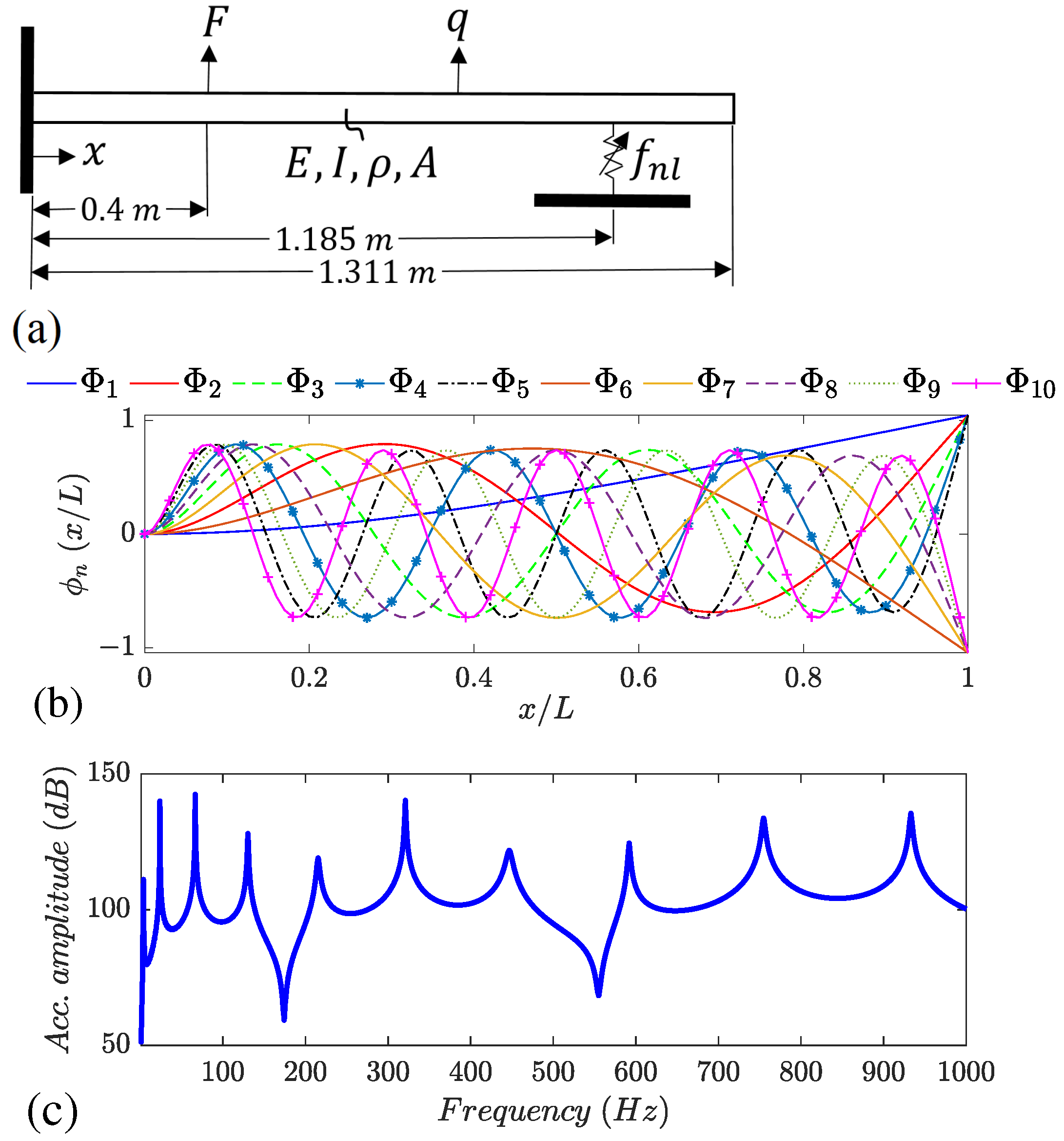
The third example is the cantilever beam problem shown in Figure 3a that has been studied widely in the nonlinear system identification literature [31,43,44]. In this example, the cantilever beam is grounded by a nonlinear stiffness spring near the beam’s free end. The beam is made of steel (with the modulus of elasticity E = 200 × 10 9 N / m 2 , and density D = 7800 N / m 3 ), is uniform and homogeneous, and has a length of 1.311 m, a width of 0.0446 m, and a thickness of 0.008 m. The damping matrix is also computed based on the classical Rayleigh damping method using mass proportional coefficient α = 0.21 , stiffness proportional coefficient β = 0.25 , where the damping ratio is ζ = 0.0045 . The beam is discretised into 100 Euler–Bernoulli beam elements, where each element consists of two nodes, each with a translational and rotational degree of freedom (DOF). Ten first mode shapes and the Fourier amplitude spectrum of the acceleration response at the tip of the beam under impulse force are shown in Figure 3b,c, respectively. It should be noted that the Fourier amplitude spectrum in Figure 3c shows the characteristics of the underlying linear system without the nonlinear stiffness element.
The type of nonlinearity considered in all of the benchmark problems is in the form of dead-zone (backlash) + polynomials, which is typically encountered in many engineering applications, especially airplane wings as a free play nonlinearity [27,28]. The parameters of the nonlinear element are set to be:
f n l = 9.05 × 10 5 | y | y + 1.05 × 10 9 ( y ) 3 + 1000 ( y ) if | q | d / 2 ; 0 if | q | < d / 2 ,
where y = q s i g n ( q ) ( d ) / 2 , d is the clearance and q is the physical displacement of the system according to Equation (1). The clearance considered in these examples is 0.002 m, so the nonlinear element activates when the response amplitude is higher than this distance.
The library of nonlinear terms used for model selection in this paper is presented in Table 2. We note that, when the dead-zone element is selected in one of the model selection iterations, the other nonlinear terms in the library are automatically updated to include the dead-zone in a piece-wise function as shown in Equation (6).
In Table 2, F f is the step force in ( N ), K f is the hardening coefficient in ( N / m ) and K d is the stiffness after contact in ( N / m ). We note that the constant value σ g = 10 7 is used here to define the transition between the two regimes of the function (term 11) in Table 2.
To generate the vibrational data, nonlinear differential equations of motions are numerically solved using the Newmark- β method. The transient response of the structure when it is vibrated using a harmonic excitation F = F 0 sin ( ω t ) is computed and used for nonlinear model identification. The amplitude of harmonic excitation is F 0 = 5 N and ω equals the natural frequency of the underlying linear structure. The sampling frequency is F s = 4480 Hz for all cases. The transient response is used as it contains information about all of the underlying fundamental features of a dynamical system, including those properties that are susceptible to change as a function of the vibration amplitude.

4. Results and Discussion

We assess the performance of the optimization methods listed in Table 1, when solving the three benchmark problems presented in Section 3. For each problem, local gradient-based and global optimisation methods are examined. The results are reported based on benchmark problems, model selection algorithms, that is, Forward–Backward (FB) and Exhaustive Search (ES). For reference, the computations were carried out using a standard desktop computer (Intel(R) Core(TM) i5-8500 CPU @ 3.00 GHz processor with 16 GB RAM).
The convergence curves for all optimization methods and the three benchmark problems using the FB algorithm are presented in Figure 4. Initially, nonlinear terms are added based on the forward approach, and then backward regression starts to eliminate the terms with less contribution to the system responses. As expected, the optimisation results indicate that the performance of the optimisation methods varies substantially among the benchmark problems. It can be seen that in almost all of the optimisation methods, between six to ten terms are initially selected by forward regression.
Some general behaviour can be observed. For instance, the decrease in the MSE values using QN, AS, TTR and PS optimisation methods are not substantial by adding terms and they do not reach the predefined stopping criteria sometimes, whereas, other algorithms reach the predefined stopping criteria for MSE by adding more terms. It can also be observed that MSE values in the initial steps of selection start from a very high value for TRR and LM and there is a sudden drop after selecting more terms, while the results of other algorithms show a smoother convergence behaviour. This can be attributed to the fact that TRR and LM try to find the correct model, and when the selected model is not yet sufficient, the minimisation does not proceed further until the next term is added to the model.
Furthermore, an interesting finding is observed in Figure 4 by comparing the results for the three different benchmark problems. Studying the convergence of the LM optimisation method as an example, it can be seen that forward regression stops after ten terms selected for the SDOF system. This is nine terms for the 3DOF system and six terms for the Cbeam system. It indicates that providing the information of coupled nonlinear modes to constrain the optimisation algorithm is helpful in selecting the correct terms in fewer iterations of the model selection algorithms.
For the quantitative evaluation, we considered CPU time as a criterion for computational effort along with the number of the cost function calls and iterations in Figure 5. In general, it can be seen that the computational effort is much lighter for the FB algorithm in comparison with ES. In addition, it is obvious that the function calls and a number of iterations are higher for ES, as it needs to cover many combinations in each iteration of the model selection algorithms. It should be noted that the number of iterations counted here is the sum of the iterations of the optimisation algorithm when estimating the parameters of each combination. Overall, the computational effort for the PS optimisation method is higher than others and LM outperforms all other algorithms in terms of efficiency with fast convergence.
In the following, we address the question of what is the best combination of optimisation method and model selection algorithm that delivers the most accurate nonlinear model. Figure 6 shows the total number of terms added to and eliminated from the nonlinear model and a final number of nonlinear terms delivered when using different optimisation methods and model selection algorithms. From Figure 6a,c,e, it can be observed that the total number of added and eliminated nonlinear terms by the FB algorithm is dropped substantially for the 3DOF and Cbeam problems in comparison with the SDOF problem. It is due to the fact that the data related to higher modes are fed into the constraint function of the optimisation algorithm when identifying the 3DOF and Cbeam problems. This observation suggests that constraining the optimisation using the data from the coupled modes improves the performance of model selection algorithms, especially the FB algorithm. The ES algorithm is less sensitive to the input data from different modes. However, observations from Figure 6e indicate that more than three terms were added to the nonlinear model of Cbeam structure using the ES algorithm. This can be attributed to the over-constraining of the optimisation algorithm as the data of nine modes are used to constrain the optimisation algorithm. This effect is explained more later in this section. It should also be mentioned that the total number of nonlinear term expansions in the ES algorithm is limited to five terms.
There is no clear difference among various optimisers in terms of a total number of added and eliminated nonlinear models. Figure 6b,d,f shows the final number of terms delivered by each model selection algorithm, and the red lines present the true number of the terms, which is three terms defined in Section 3. It can be seen that forward regression is not able to deliver the correct number of terms and the results demonstrate a comparable performance among the optimisers. Only QN and LM optimisers were able to achieve the correct number of terms (three terms) when using the FB algorithm and the others have almost delivered a comparable final number of terms. The number of delivered terms using the ES algorithm is correct for most of the cases and there are just a few optimisers that selected more terms in the case of Cbeam, which is due to the high number of modes used to constrain the optimisation method. Therefore, this performance evaluation suggests the use of LM for model selection.
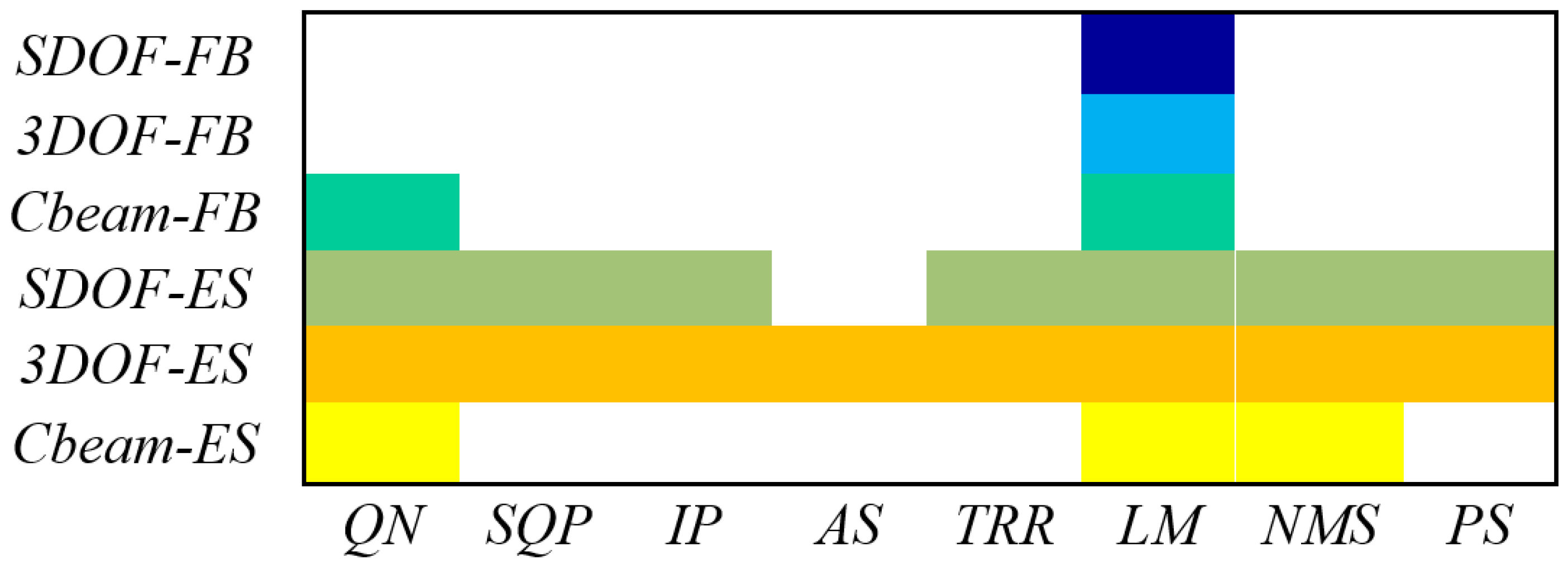
Figure 7 shows the methods that successfully solved the benchmark problems. The color tiles indicate that the search method delivered the true nonlinear model and parameters; white tiles indicate methods that were not able to deliver the true model as defined in Section 3. It can be seen that, for the BF algorithm, only the LM optimiser was successful at delivering the true model for all of the benchmark problems. Most of the optimisers are successful to deliver the true nonlinear model using the ES algorithm.
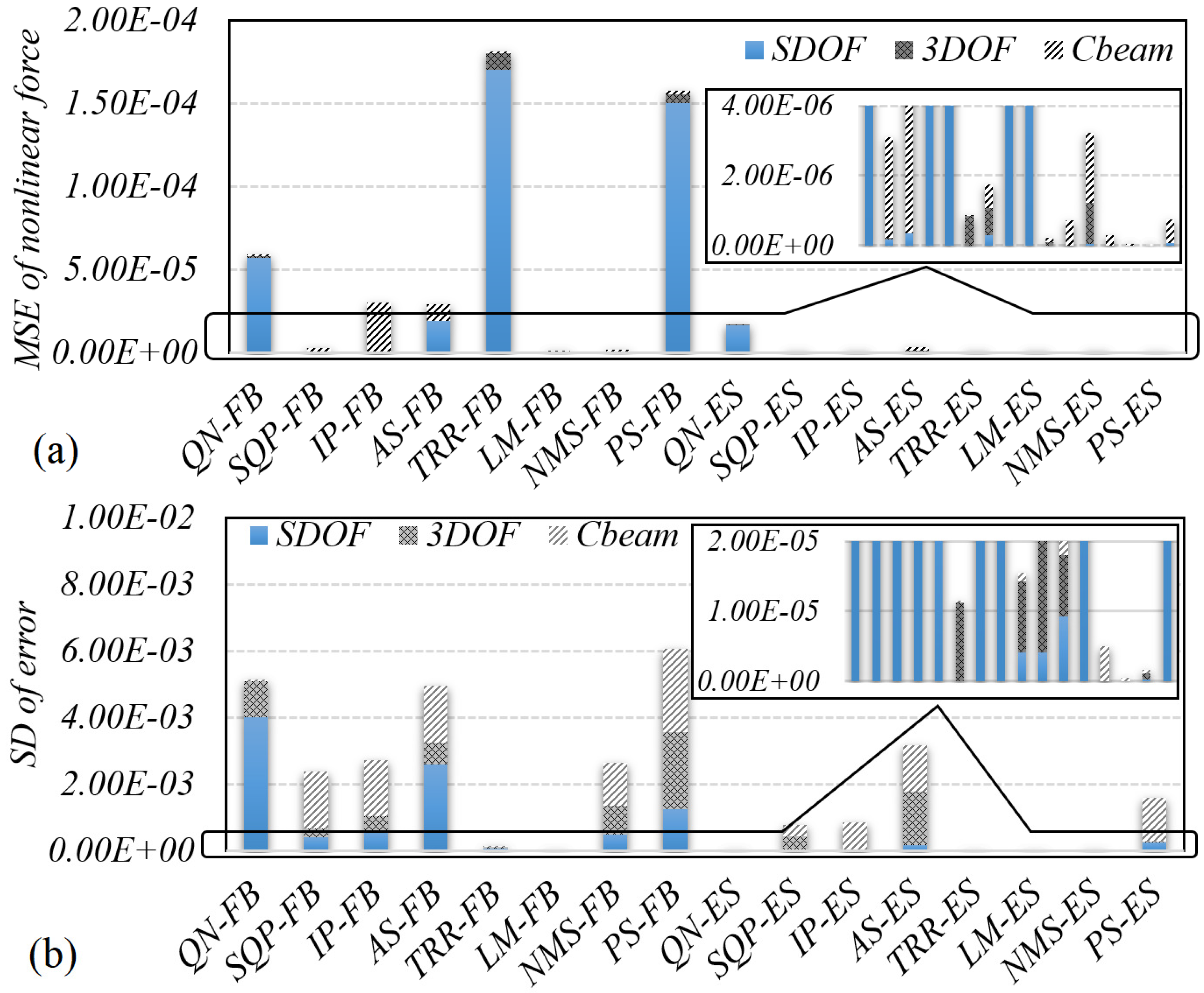
Figure 8 shows the MSE values and standard deviation (SD) of error for the delivered model considering all of the employed optimisation methods. The MSE value is computed based on the error of estimated and true nonlinear force using Equation (4). It can be seen that the MSE and standard deviation of error are low for TRR and LM in comparison with the other methods. As a result, LM demonstrates high performance in terms of estimating the true parameters correctly. The comparison of all methods reveals that LM possesses the best overall efficiency and accuracy on the considered benchmark problems and settings.
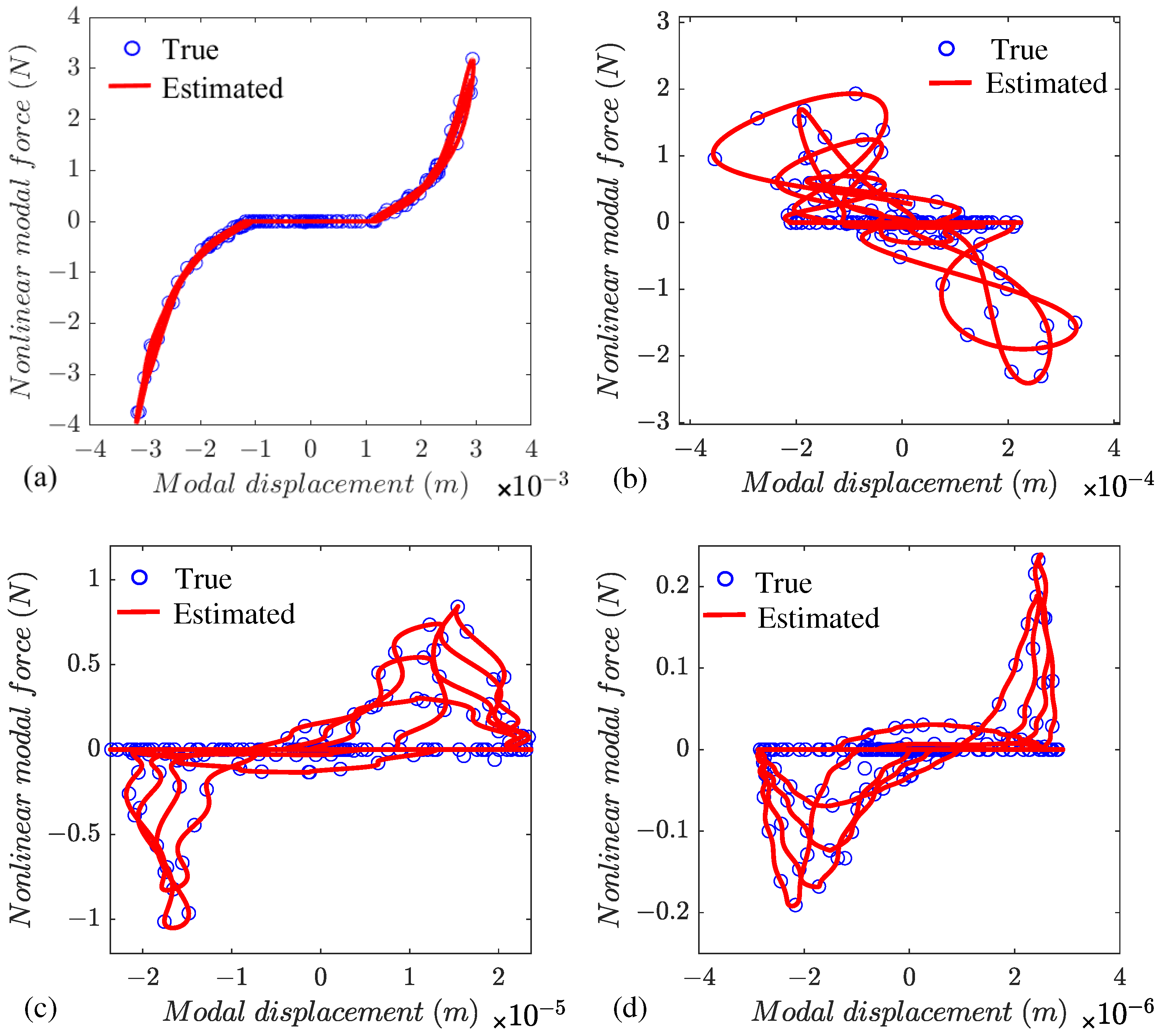
Here, we provide some insight into the nonlinear model selection of a cantilever beam. The responses of the ten first modes are considered in the model selection process as described in Section 2.1. The first mode is considered in the optimization process as the main mode and the other nine first modes are considered as constraint modes (Equation (4)). The modal nonlinear force of four first mode is shown in Figure 9. It can be seen that the contribution of higher modes in the response due to nonlinear modal coupling is low. Just considering a limited number of important modes will be enough to help the optimisation algorithm in working out the parameters and the best nonlinear model. In other words, modes with negligible contributions might have adverse effects on the model selection process as those data have relatively less useful information if compared with other modes, but increase computational effort.

Performance of Hybrid Optimisation Methods

Based on the study above, we further examined the performance of MS-LM and hybrid (PS-LM) optimisation methods (Table 1) for nonlinear model selection. The SDOF system used for this assessment and the results are reported in Table 3. Comparable accuracy is expected for both multi-start and hybrid approaches since LM alone provides a good solution for this specific example. Some insight can also be initiated by the nature of these two different approaches. As can be seen, MS-LM is successful in finding the correct nonlinear terms with high accuracy and PS-LM is failed to find the correct terms based on the FB algorithm. However, the selected model by PS-LM has passed the stopping criteria to be an acceptable model.
The difference between the results of MS-LM and PS-LM can be attributed to the way they treat the optimisation problem. First of all, the optimisation problem is defined as described in Section 2.1, where the nonlinear parameters are scaled and bounded. The MS-LM method starts the LM gradient based method from different randomly generated initial points in the search space. This way, MS-LM ends up in a different basin of attractions and finally finds the minimum of all local searches. The reported minimum value is considered as a global minimum. On the other hand, the PS optimisation method starts from randomly generated initial points and the generated swarm moves toward the minimum in the search space. When the swarm reaches a minimum and the PS optimisation method stops proceeding, it passed the minimum point information to the LM method. Afterwards, the LM method starts searching from the minimum initial point provided by the PS optimisation method. It should be noted that the basin of attraction that is found by the PS optimisation method is not guaranteed to include the global minimum of the search space for an n-dimensional cost function. Therefore, the LM method might not find the global minimum in the basin of attraction prescribed by the PS optimisation method. As a result, hybrid methods can potentially outperform the efficiency (convergence rate) of the multi-start method while keeping their success rate. However, the results reported here show that the MS method reaches a more accurate nonlinear model selection and parameter estimation.

5. Conclusions

This paper presents a comparative evaluation of ten optimization methods for nonlinear model selection and parameter estimation of nonlinear dynamic systems. Three problems of different levels of complexities, each considering effectively the contribution of one, two, and ten modal responses, have been examined. The nonlinear model selection has been carried out using two different data-driven algorithms, that is, forward–backward and exhaustive search algorithms. They have been used to select the best possible nonlinear model from a predefined library of nonlinear terms and estimate its parameters. The time domain vibration response data of the system were directly used as an input to the model selection algorithms. A multi-criteria workflow was presented to compare different local and global optimisation methods based on their performance in terms of efficiency and accuracy. The properties of the underlying linear system and maxima of the system’s dynamic responses were used to scale the search space of the defined optimisation problem. The parameters of nonlinear models were also bounded in the scaled space to reflect physically meaningful behaviour. From a practical point of view, the FB algorithm is efficient in terms of computational time and accuracy for structures with many nonlinear elements and terms. The ES algorithm is more applicable for structures with limited nonlinear elements as it could generate a huge number of combinations depending on the size of the predefined library of nonlinear terms. Initially, gradient-based optimisation methods, along with NMS and PSO algorithms, were evaluated. The results show that gradient-based methods are efficient and accurate for nonlinear model selection problems. In particular, the LM optimisation method outperforms all the other methods considered in this study when finding the best model for the nonlinearity with a low computational effort. Based on the results from the initial evaluation, the nonlinear model selection was performed using the MS-LM and PSO-LM methods. Both of these methods were successful in fitting a nonlinear model with high accuracy and a comparable run time. However, the MS-LM outperforms the hybrid PSO-LM in finding a true predefined model. This is attributed to the nature of MS and PSO methods. MS starts from different randomly generated initial points in the search space and considers an equal chance for all of them, whereas PSO finds a basin of attraction with a local minimum and initiates the local gradient-based method, that is, LM within that basin. Therefore, these two hybrid methods are recommended to be used in practice for the nonlinear model identification of engineering structures.
It is noteworthy that multiple time series (e.g., data from several vibration tests) will need to be used in order to quantify the uncertainty of the nonlinear identification framework studied in this paper. This will provide evidence of how reliable the nonlinear model identification method is. This challenging topic is currently under study but remains unsolved. Similarly, we note that the data-driven nonlinear system identification strategy used here can be further improved, for instance, by using statistical tools to assess the model parsimony; nonetheless, as all optimisation algorithms presented here solved exactly the same optimisation problem (with the respective decision rules and constrains), the results presented above in terms of differences in the optimisation algorithms performance is unlikely to change, that is, the final solution (model selected) might be different but the comparative performance of the optimisation algorithms will remain essentially the same. Furthermore, the model selection algorithms could be vastly sped up by taking advantage of multi-core processors and parallel computing.

Author Contributions

Conceptualization, S.S. and J.L.M.; methodology, S.S. and J.L.M.; software, S.S. and J.L.M.; validation, S.S. and J.L.M.; formal analysis, S.S.; investigation, S.S. and J.L.M.; resources, S.S. and J.L.M.; data curation, S.S.; writing—original draft preparation, S.S.; writing—review and editing, S.S. and J.L.M.; visualization, S.S.; supervision, J.L.M.; project administration, J.L.M.; funding acquisition, J.L.M. All authors have read and agreed to the published version of the manuscript.

Funding

This research received no external funding.

Data Availability Statement

Not applicable.

Acknowledgments

Safari is support by the scholarship from the College of Engineering, Mathematics, and Physical Sciences, University of Exeter which is gratefully acknowledged.

Conflicts of Interest

The authors declare no conflict of interest.

References

  1. Ondra, V.; Riethmueller, R.; Brake, M.R.W.; Schwingshackl, C.W.; Polunin, P.M.; Shaw, S.W. Comparison of Nonlinear System Identification Methods for Free Decay Measurements with Application to MEMS Devices. In Sensors and Instrumentation; Sit, E.W., Walber, C., Walter, P., Seidlitz, S., Eds.; Springer: Cham, Switzerland, 2017; Volume 5. [Google Scholar]
  2. Noël, J.; Marchesiello, S.; Kerschen, G. Subspace-based identification of a nonlinear spacecraft in the time and frequency domains. Mech. Syst. Signal Process. 2014, 43, 217–236. [Google Scholar] [CrossRef]
  3. Dossogne, T.; Masset, L.; Peeters, B.; Noël, J. Nonlinear dynamic model upgrading and updating using sine-sweep vibration data. Proc. R. Soc. A 2019, 475, 20190166. [Google Scholar] [CrossRef]
  4. Ewins, D. Modal Testing: Theory, Practice, and Application; Engineering Dynamics Series; John Wiley & Sons: Hoboken, NJ, USA, 2000. [Google Scholar]
  5. Dou, S.; Jensen, J. Optimization of hardening/softening behavior of plane frame structures using nonlinear normal modes. Comput. Struct. 2016, 164, 63–74. [Google Scholar] [CrossRef] [Green Version]
  6. Liao, H. An approach to construct the relationship between the nonlinear normal mode and forced response of nonlinear systems. J. Vib. Control 2016, 22, 3169–3181. [Google Scholar] [CrossRef]
  7. Sombroek, C.; Tiso, P.; Renson, L.; Kerschen, G. Numerical computation of nonlinear normal modes in a modal derivative subspace. Comput. Struct. 2018, 195, 34–46. [Google Scholar] [CrossRef] [Green Version]
  8. Prawina, J.; Rao, A.; Lakshmi, K. Nonlinear identification of structures using ambient vibration data. Comput. Struct. 2015, 154, 116–134. [Google Scholar] [CrossRef]
  9. Noël, J.; Kerschen, G. Nonlinear system identification in structural dynamics: 10 more years of progress. Mech. Syst. Signal Process. 2017, 83, 2–35. [Google Scholar] [CrossRef]
  10. Brunton, S.; Kutz, J. Data-Driven Science and Engineering: Machine Learning, Dynamical Systems, and Control; Cambridge University Press: Cambridge, UK, 2019. [Google Scholar]
  11. Wright, J.; Cooper, J.; Desforges, M. Normal-mode force appropriation-theory and application. Mech. Syst. Signal Process. 1999, 13, 217–240. [Google Scholar] [CrossRef]
  12. Kerschen, J.; Golinval, J.; Worden, K. Theoretical and experimental identification of a non-linear beam. J. Sound Vib. 2001, 244, 597–613. [Google Scholar] [CrossRef] [Green Version]
  13. Marchesiello, S.; Garibaldi, L. A time domain approach for identifying nonlinear vibrating structures by subspace methods. Mech. Syst. Signal Process. 2008, 22, 81–101. [Google Scholar] [CrossRef]
  14. Billings, S. Nonlinear System Identification: NARMAX Methods in the Time, Frequency and Spatio-Temporal Domains; Wiley: Hoboken, NJ, USA, 2013. [Google Scholar]
  15. Karaağaçlı, T.; Özgüven, H.N. Experimental Identification of Backbone Curves of Strongly Nonlinear Systems by Using Response-Controlled Stepped-Sine Testing (RCT). Vibration 2020, 3, 266–280. [Google Scholar] [CrossRef]
  16. Londoño, J.; Neild, S.; Cooper, J. Identification of backbone curves of nonlinear systems from resonance decay responses. J. Sound Vib. 2015, 348, 224–238. [Google Scholar] [CrossRef] [Green Version]
  17. Londoño, J.; Cooper, J.; Neild, S. Identification of systems containing nonlinear stiffnesses using backbone curves. Mech. Syst. Signal Process. 2017, 84, 116–135. [Google Scholar] [CrossRef] [Green Version]
  18. Moore, K. Characteristic nonlinear system identification: A data-driven approach for local nonlinear attachments. Mech. Syst. Signal Process. 2019, 131, 335–347. [Google Scholar] [CrossRef]
  19. Mangan, N.M.; Kutz, J.N.; Brunton, S.L.; Proctor, J.L. Model selection for dynamical systems via sparse regression and information criteria. Proc. R. Soc. A 2017, 473. [Google Scholar] [CrossRef] [Green Version]
  20. Paduart, J.; Lauwers, L.; Swevers, J.; Smolders, K.; Schoukens, J.; Pintelon, R. Identification of nonlinear systems using polynomial nonlinear state space models. Automatica 2010, 46, 647–657. [Google Scholar] [CrossRef]
  21. Balaji, N.N.; Lian, S.; Scheel, M.; Brake, M.R.W.; Tiso, P.; Noël, J.P.; Krack, M. Numerical Assessment of Polynomial Nonlinear State-Space and Nonlinear-Mode Models for Near-Resonant Vibrations. Vibration 2020, 3, 320–342. [Google Scholar] [CrossRef]
  22. Cooper, S.; Tiels, K.; Tituruse, B.; DiMaio, D. Polynomial nonlinear state space identification of an aero-engine structure. Comput. Struct. 2020, 238, 106299. [Google Scholar] [CrossRef]
  23. Worden, K.; Barthorpe, R.; Cross, E.; Dervilis, N.; Holmes, G.; Manson, G.; Rogers, T. On evolutionary system identification with applications to nonlinear benchmarks. Mech. Syst. Signal Process. 2018, 112, 194–232. [Google Scholar] [CrossRef]
  24. Abdessalem, A.B.; Dervilis, N.; Wagg, D.; Worden, K. Model selection and parameter estimation in structural dynamics using approximate Bayesian computation. Mech. Syst. Signal Process. 2018, 99, 306–325. [Google Scholar] [CrossRef]
  25. Taghipour, J.; Khodaparast, H.; Friswell, M.; Jalali, H. An Optimization-Based Framework for Nonlinear Model Selection and Identification. Vibration 2019, 2, 311–331. [Google Scholar] [CrossRef] [Green Version]
  26. Safari, S.; Londoño, J. Direct optimisation based model selection and parameter estimation using time-domain data for identifying localised nonlinearities. J. Sound Vib. 2021, 51, 116056. [Google Scholar] [CrossRef]
  27. Roberts, I.; Jones, D.; Lieven, N.; di Bernado, M.; Champneys, A. Analysis of piecewise linear aeroelastic systems using numerical continuation. Proc. Inst. Mech. Eng. Part G J. Aerosp. Eng. 2002, 216, 747–763. [Google Scholar] [CrossRef] [Green Version]
  28. Baea, J.S.; Inmana, D.; Leeb, I. Effects of structural nonlinearity on subsonic aeroelastic characteristics of an aircraft wing with control surface. J. Fluids Struct. 2004, 19, 747–763. [Google Scholar] [CrossRef]
  29. Clough, R.; Penzien, J. Dynamics of Structures; Computers and Structures, Inc.: Berkeley, CA, USA, 2003. [Google Scholar]
  30. Peeters, P.; Auweraera, H.; Guillaumeb, P.; Leuridana, J. The PolyMAX frequency-domain method: A new standard for modal parameter estimation? Shock Vib. 2004, 11, 395–409. [Google Scholar] [CrossRef]
  31. Moore, K.; Kurt, M.; Eriten, M.; McFarland, M.; Bergman, L.; Vakakis, A. Direct detection of nonlinear modal interactions from time series measurements. Mech. Syst. Signal Process. 2019, 125, 311–329. [Google Scholar] [CrossRef]
  32. Moore, K.; Kurt, M.; Eriten, M.; McFarland, M.; Bergman, L.; Vakakis, A. Time-series-based nonlinear system identification of strongly nonlinear attachments. J. Sound Vib. 2019, 438, 13–32. [Google Scholar] [CrossRef]
  33. Safari, S.; Londoño, J. Nonlinear Function Selection and Parameter Estimation of Structures with Localised Nonlinearities, Part 1: Numerical Analysis. In Nonlinear Structures and Systems; Kerschen, G., Brake, M., Renson, L., Eds.; Springer: Cham, Switzerland, 2019; Volume 1. [Google Scholar]
  34. Akaike, H. A new look at the statistical model identification. IEEE Trans. Autom. Control 1974, 19, 716–723. [Google Scholar] [CrossRef]
  35. Schittkowski, K. Numerical Data Fitting in Dynamical Systems: A Practical Introduction with Applications and Software, 1st ed.; Springer Science and Business Media: Dordrecht, The Netherlands, 2013; Volume 77. [Google Scholar]
  36. Isermann, R.; Munchhof, M. Identification of Dynamic Systems, An Introduction with Applications; Springer: Berlin/Heidelberg, Germany, 2011. [Google Scholar]
  37. Kennedy, J.; Eberhart, R. Particle swarm optimization. In Proceedings of the ICNN’95—International Conference on Neural Networks, Perth, Australia, 27 November–1 December 1995; Volume 4, pp. 1942–1948. [Google Scholar]
  38. Das, S.; Mondal, S.; Guchhait, S. Particle swarm optimization–based characterization technique of nonproportional viscous damping parameter of a cantilever beam. J. Vib. Control 2021, 10775463211010526. [Google Scholar] [CrossRef]
  39. Martí, R.; Corberán, Á.; Peiró, J. Scatter Search. In Handbook of Heuristics; Martí, R., Panos, P., Resende, M.G., Eds.; Springer International Publishing: Cham, Switzerland, 2016; pp. 1–24. [Google Scholar] [CrossRef]
  40. Zhigljavsky, A.; Zilinskas, A. Stochastic Global Optimization, 1st ed.; Springer Optimization and Its Applications; Springer: Berlin/Heidelberg, Germany, 2008; Volume 9. [Google Scholar]
  41. Piotrowski, A.; Napiorkowski, J.; Piotrowska, A. Population size in Particle Swarm Optimization. Swarm Evol. Comput. 2020, 58, 100718. [Google Scholar] [CrossRef]
  42. Villaverde, A.F.; Fröhlich, F.; Weindl, D.; Hasenauer, J.; Banga, J.R. Benchmarking optimization methods for parameter estimation in large kinetic models. Bioinformatics 2019, 35, 830–838. [Google Scholar] [CrossRef] [PubMed]
  43. Kurt, M.; Chen, H.; Lee, T.; McFarland, D.; Bergman, L.; Vakakis, A. Nonlinear system identification of the dynamics of a vibro-impact beam: Numerical results. Arch. Appl. Mech. 2012, 82, 1461–1479. [Google Scholar] [CrossRef] [Green Version]
  44. Herrera, C.A.; McFarland, D.; Bergma, L.; Vakakis, A. Methodology for nonlinear quantification of a flexible beam with a local, strong nonlinearity. J. Sound Vib. 2017, 388, 298–314. [Google Scholar] [CrossRef]
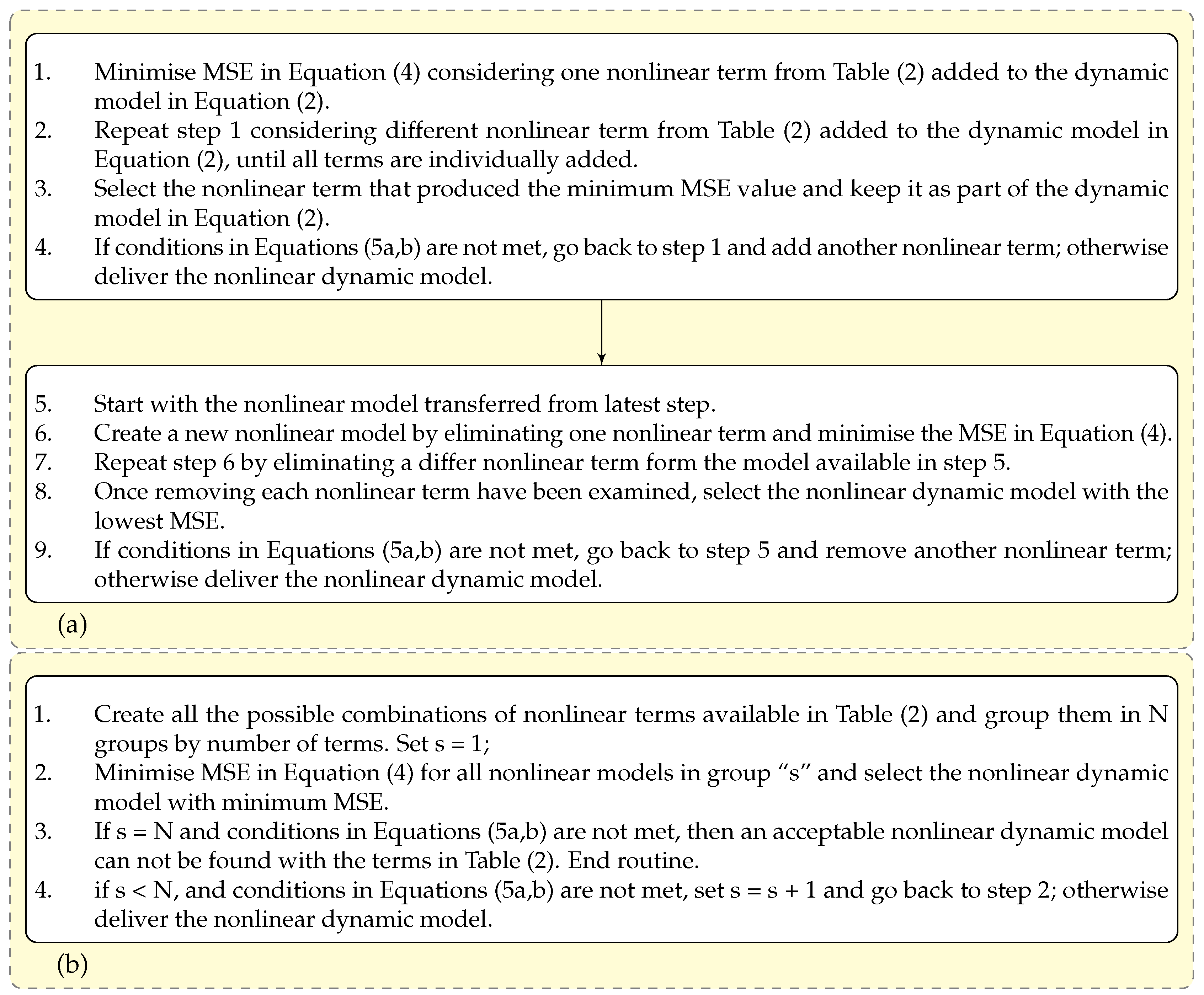
Figure 1. Nonlinear model selection algorithms (a) FB, (b) ES (adapted from [26]).
Vibration 04 00036 g001
Figure 2. Discrete system benchmark problems (a) SDOF, (b) MDOF with one nonlinear element.
Vibration 04 00036 g002
Figure 3. Cantilever beam with a nonlinear attachment benchmark (a) configuration, (b) the first ten normalized mode shape functions ϕ n ( x / L ) , (c) Amplitude spectrum of acceleration response at the tip of the beam.
Vibration 04 00036 g003
Figure 4. Model selection convergence curves for FB algorithm for the cases: (a) SDOF, (b) 3DOF, (c) Cbeam systems.
Vibration 04 00036 g004
Figure 5. Efficiency criteria of optimisation methods for nonlinear model selection (a) CPU time, (b) function calls, (c) number of iterations; (*: the number of vertical axes should be multiplied by ten).
Vibration 04 00036 g005
Figure 6. Evaluation of the number of terms processed by model selection algorithm using different optimisation methods (a) SDOF terms added and removed, (b) SDOF number of terms delivered, (c) 3DOF terms added and removed, (d) 3DOF number of terms delivered, (e) Cbeam terms added and removed, (f) Cbeam number of terms delivered; (The red dashed lines present the true number of the terms).
Vibration 04 00036 g006
Figure 7. Delivering the true nonlinear model for each benchmark. Color tiles: successful; white tiles: unsuccessful at delivering the true model.
Vibration 04 00036 g007
Figure 8. Accuracy of the delivered model using different optimisation methods in predicting the response (a) MSE of nonlinear force; (b) standard deviation (SD) of error.
Vibration 04 00036 g008
Figure 9. Nonlinear modal force-displacement responses fitted based on LM optimisation algorithm (a) mode 1, (b) mode 2, (c) mode 3, (d) mode 4.
Vibration 04 00036 g009
Table 1. Classification of optimisation methods considered in the benchmarking.
Global MethodsLocal Methods
Nelder–Mead Simplex (NMS)Quasi-Newton (QN)
Particle Swarm (PS)Sequential Quadratic Programming (SQP)
Particle Swarm (PS) + local methodActive-Set (AS)
Multi-start (MS) + local methodInterior Point (IP)
Trust-Region-Reflective (TRR)
Levenberg-marquardt (LM)
Table 2. Nonlinear terms considered in the library.
No.Nonlinear Term f nl ( q ) No.Nonlinear Term f nl ( q )
1 | q | q 7 sign ( q ) | q |
2 q 3 8 q | q |
3 | q | q 3 9 | q | q | q |
4 q 5 10 q 3 | q |
5 | q | q 5 11 F f 2 1 + e ( σ g q ) 1 + K f q
6 q 7 12 K d q sign ( q ) d 2 if | q | d / 2
0 if | q | < d / 2
Table 3. Parameters assigned for nonlinearities in the example SDOF systems.
CriteriaSDOF-FBSDOF-ES
MS-LMPS-LMMS-LMPS-LM
CPU time (sec)6652516820275248
MSE 5 × 10 13 4 × 10 7 6 × 10 13 4 × 10 8
SuccessYesNoYesYes
Publisher’s Note: MDPI stays neutral with regard to jurisdictional claims in published maps and institutional affiliations.