Article

Experimental Characterization of Friction in a Negative Stiffness Nonlinear Oscillator

by
Dario Anastasio
and
Stefano Marchesiello
*
Department of Mechanical and Aerospace Engineering, Politecnico di Torino, Corso Duca degli Abruzzi 24, 10129 Torino, Italy
*
Author to whom correspondence should be addressed.
Vibration 2020, 3(2), 132-148; https://doi.org/10.3390/vibration3020011
Submission received: 15 May 2020 / Revised: 1 June 2020 / Accepted: 3 June 2020 / Published: 5 June 2020
(This article belongs to the Special Issue Data-Driven Modelling of Nonlinear Dynamic Systems)

Abstract

:
Nonlinear dissipative phenomena are common features of many dynamical systems and engineering applications, and their experimental characterization has always been a challenge among the research community. Within the wide range of nonlinear damping mechanisms, friction is surely one of the most common, and with a high impact on the dynamical behavior of structures. In this paper, the nonlinear identification of friction in a negative stiffness oscillator is pursued. The structure exhibits a strong nonlinear behavior, mainly due to its polynomial elastic restoring force with a negative stiffness region. This leads to an asymmetric double-well potential with two stable equilibrium positions, and the possibility of switching between them in a chaotic way. Friction plays a crucial role in this context, as it derives from the continuous sliding between the central guide and the moving mass. The system is driven through harmonic tests with several input amplitudes, in order to estimate the variations in the energy dissipated per cycle. The identification of the frictional behavior is then pursed by minimizing the errors between the experimental measurements and the model predictions, using the harmonic balance method in conjunction with a continuation technique on the forcing amplitudes.

1. Introduction

Friction is a complex nonlinear phenomenon highly present in mechanical systems. It results from the interaction between adjacent surfaces and is dependent on their topography and materials, and on the presence of lubrication and relative motion [1]. Studies on friction have been carried out for more than 500 years [2], and a more detailed explanation about modeling techniques can be found in several works in the literature [3,4,5]. A major classification of friction is usually done by separating the “pre-sliding” from the “sliding” (or “gross-sliding”) behavior. The first can be associated with the elastic and plastic deformations at the asperity levels of the adjacent surfaces, and it is known to be mostly dependent on their relative displacement. The friction force in the pre-sliding regime is a hysteretic function of the position with a non-local memory [1,4]. Instead, the sliding regime is largely due to the shearing resistance of the asperities, and mainly dependent on the velocity. The pioneering friction model of Coulomb [6] is indeed the most known example of sliding friction.
The experimental identification of friction has always been a difficult task, especially when real-life mechanical structures are involved. This is indeed due to the intrinsic nonlinear nature of the friction phenomenon, which may lead to limit cycles, tracking errors, stick–slip motion, hysteresis and other typical features of nonlinear systems such as natural frequency shifts and jumps. Many nonlinear identification techniques have been developed by the research community in the last decades, and two extensive literature reviews can be found in [7,8]. Nevertheless, different methods are suitable for the different classes of nonlinearities and kind of excitations, and few of them have been tested with frictional and/or hysteresis nonlinearities. In [1], several identification techniques of pre-sliding and sliding friction were compared, ranging from white-box to black-box models. The identifications were performed directly on the friction force, which was measured in a controlled laboratory setup with a tribometer. In [9], the same experimental setup was adopted and the identification was performed considering the LuGre [10] and the Maxwell-slip [11] friction models in conjunction with nonlinear regression techniques. The LuGre model was again adopted in [12] to identify the frictional behavior in a torque motor control system, using an evolutionary algorithm to minimize the residuals between predictions and measurements with constant velocity experiments. A different approach was adopted in [13], where a general hysteresis model was identified via the nonlinear state–space modeling of a single-degree-of-freedom system under multisine excitation. Ground vibrations sine sweep tests were conducted in [14], to estimate the shape of the friction force at the joints of the wing-payload substructure of an F-16 aircraft using the restoring force surface (RFS) [15] and wavelet transform methods. Indeed, friction phenomena associated with joints are known to be a typical source of nonlinearity in mechanical systems [16], and this represents a critical issue in several engineering applications, such as bladed disks [17]. In such cases, friction is usually modeled with node-to-node contact elements, where Coulomb’s friction law is used to model the local slip conditions of the joint interfaces [18]. On the experimental side, the nonlinear dynamical behavior of contact interfaces has been widely observed, for instance in [19,20,21].
In this paper, the data-driven nonlinear modeling of the frictional behavior of a negative stiffness oscillator is performed. The oscillator is part of a device designed to improve the current collection quality in railway overhead contact lines, attempting to alter their damping distribution and reduce the wave propagation, known to be a critical phenomenon in such structures [22,
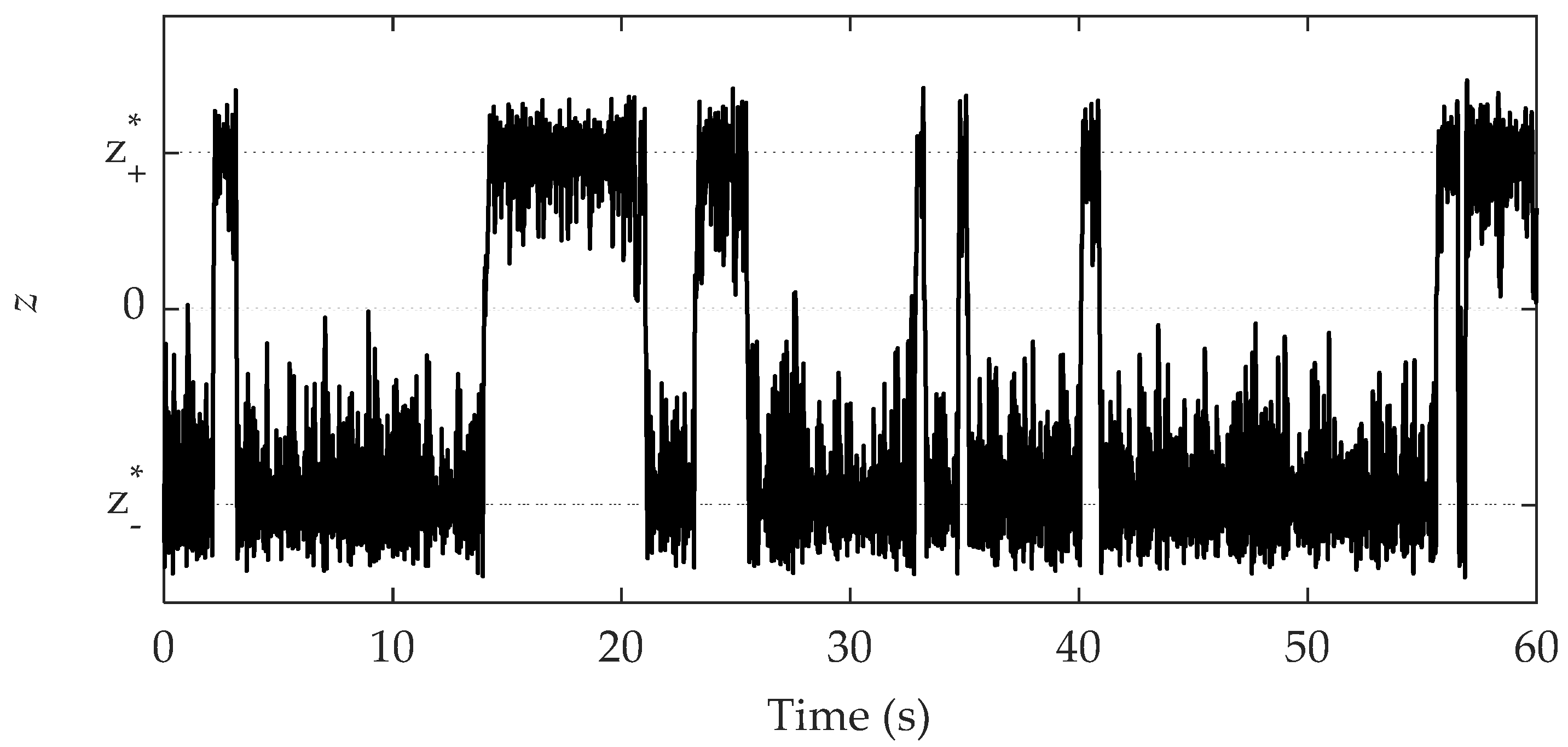
23]. It is characterized by a strong nonlinear behavior mainly due to its double-well characteristics [24], and it exhibits two stable equilibrium positions plus an unstable one. The oscillations can either be bounded around one stable point (“in-well”) or include all the three positions (“cross-well”). In both cases, periodic oscillations can evolve to steady in-well or cross-well chaotic motions under external periodic excitations [25,26]. The bi-stable nature of the device is translated to a polynomial-kind restoring force with a negative slope around the origin. This has been experimentally identified in a previous work [27] using the nonlinear subspace identification method (NSI) [28] with cross-well oscillations under random excitation. However, the method struggled when trying to infer a nonlinear dissipative model.
The identification of the friction force of the device turns out to be a particularly challenging task, as it is not the only and dominant source of nonlinearity. The device is here driven through several harmonic excitations with increasing amplitudes, and the friction force is identified by minimizing the residuals between the model predictions and experimental measurements of the energy dissipated per cycle over the considered input amplitude range. The model response is computed using the harmonic balance method (HBM) [29], therefore searching for periodic responses approximated by Fourier series. HBM is usually adopted in conjunction with a continuation technique [30,31] to study the evolution of the periodic solutions with respect to the excitation frequency and to build the so-called “nonlinear frequency response curves”. The same idea is used in this paper, but a novel procedure is implemented adopting the continuation technique with respect to the excitation amplitude. This allows to estimate the “nonlinear amplitude response curves”, and therefore the dissipated energy per cycle. Given the interest in obtaining a physically based model, a white-box approach is pursued in this work. A proper frictional model should then be considered, which is first inferred using the RFS method together with physical insights about the device functionality. A genetic algorithm [32] is eventually used to optimize the model parameters based on the experimental observations.
Results show a good confidence in the identified parameters and provide a reliable model able to catch the strong nonlinear dynamics of the structure under test. This confirms the effectiveness of the presented methodology, which can be applied to a wide class of nonlinear systems.

2. A Negative Stiffness Oscillator

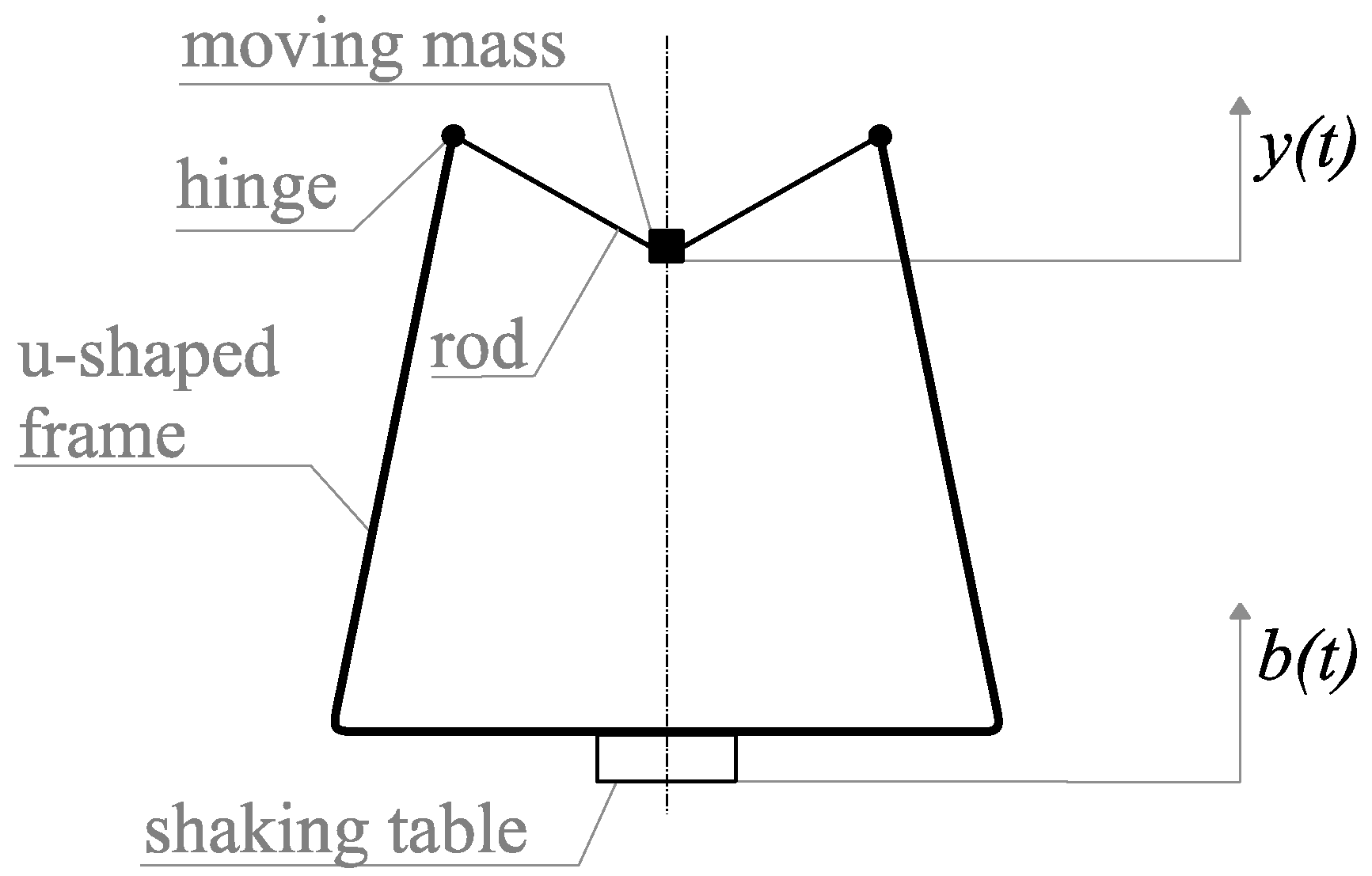
The device consists of a U-shaped frame connected through rods to a central moving mass. The frame keeps the rods under compression during their movement, achieving a bi-stable mechanism. A schematic representation of the device is depicted in Figure 1.
The lower surface of the frame is attached to a shaking table, so as to impose a displacement b ( t ) to the structure. An accelerometer is located on the shaking table to measure the acceleration of the base b ¨ ( t ) . The displacement b ( t ) is then obtained by integrating twice its measured acceleration. It is also assumed that the inertia of the moving parts can be concentrated into one central point with a mass of m = 0.26   kg , comprising the mass of the central bushing and the equivalent inertia of the rods. The vertical movement of this point is described by the coordinate y ( t ) and it is measured by a laser vibrometer. The zero position of y ( t ) corresponds to the horizontal configuration of the rods. The reader can refer to [27] for more details about the device.
It is assumed that the system can be modeled as a single-degree-of-freedom system in the variable z ( t ) = y ( t ) b ( t ) , leading to an equation of motion of the kind
m z ¨ + ( z , z ˙ ) = m b ¨ = f ( t ) ,
where   ( z , z ˙ ) is the restoring surface, the sum of the (elastic) restoring force K ( z ) and the damping force D ( z , z ˙ ) . The latter is supposed to be a function of both displacement z and velocity z ˙ . The restoring force of the considered system can be expressed as a polynomial expansion of degree three:
K ( z ) = k 3 z 3 + k 2 z 2 k 1 z + k 0 .
Therefore, the undamped equation of motion takes the form of a double-well asymmetric Duffing oscillator [
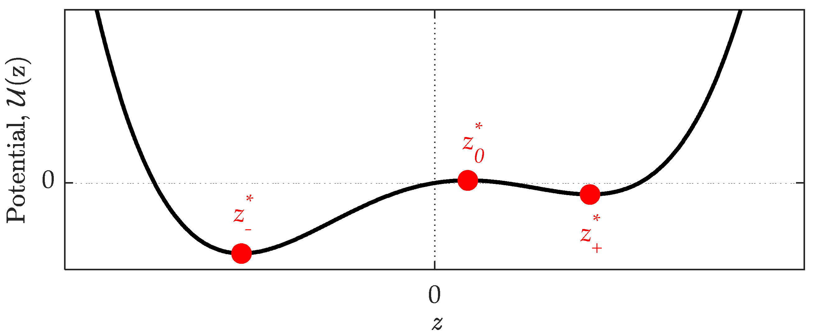
26], and its potential can be defined as
U ( z ) = 1 4 k 3 z 4 + 1 3 k 2 z 3 1 2 k 1 z 2 + k 0 z .
A qualitative representation of the potential is shown in Figure 2, where its double-well nature can be clearly noticed. The potential is not symmetric because of the gravitational contribution and the asymmetry of the frame. Further, the three equilibrium positions are depicted, obtained by setting K ( z * ) = 0 . Two out of three positions represent a stable equilibrium, namely z * and z + * , while the central position z 0 * is an unstable equilibrium point. The oscillations of the moving point are said to be “in-well” when the motion is bounded around one of the two stable equilibrium positions z ± * . The associated linear natural frequency ω ± can be computed by
ω ± = U ( z ± * ) m ,
U ( z ± * ) being the second derivative of U ( z ) computed in z * or z + * .
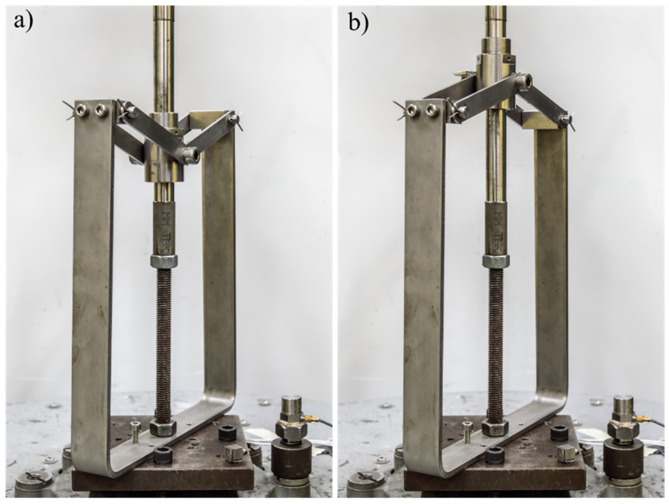
Two photos of the device in correspondence with the two stable equilibrium positions are depicted in Figure 3.

3. Experimental Nonlinear Characterization and Equation of Motion

Both random and harmonic tests have been performed to identify the features of the device, and all the tests have been conducted with a sampling frequency of 512 Hz . In particular, random tests have been used in a prior work to identify the restoring force of the device, whose results are briefly summarized in the following. Harmonic tests are instead used in this work to identify the damping force. The excitation force is expressed in this case in terms of excitation amplitude f 0 and frequency ν .

3.1. Identification of the Restoring Force

The values of the coefficients of the restoring force have been experimentally identified in [27] using the nonlinear subspace identification (NSI) algorithm with cross-well measurements under random excitation. A portion of the time history of the measured displacement z ( t ) is reported in Figure 4, while the identified values are reported in Table 1.
According to Equation (4), the linear natural frequencies of the small oscillations around the two stable equilibrium positions are ω = 11.6 2 π   rad / s and ω + = 8.6 2 π   rad / s .
The RFS method can be applied to the time history of Figure 4 to visualize the experimental restoring and damping forces, and the results are depicted in Figure 5a. In particular, if small velocities are taken into account, such that | z ˙ | < ϵ s , the obtained slice of the restoring surface approximates the restoring force K . Figure 5b shows the experimental restoring force compared to the identified one of Table 1, which nicely fits the experimental observations. Instead, when small displacements around the equilibrium positions are considered, such that | z z * | < ϵ d , an approximation of the damping force D should be retrieved. This is reported in Figure 5c, but the dispersion of the points appears to be too high to correctly deduce any damping model.

3.2. Characterization of the Friction Force

Given the difficulty of extrapolating a damping model from random measurements, two series of stepped sine tests have been performed with increasing forcing input amplitudes at a fixed excitation frequency of ν = 9   Hz , starting from the two equilibrium positions. An extract of the recorded displacement is depicted in Figure 6.
The two measured responses are then stacked together to build the experimental restoring surface, illustrated in Figure 7a. As before, if small velocities are taken into account ( | z ˙ | < ϵ s ), the obtained slice of the restoring surface approximates the restoring force K (Figure 7b), and the results are comparable with Figure 5b. The experimental damping force D is depicted in Figure 7c and obtained considering small displacements around the equilibrium positions ( | z z * | < ϵ d ). The results in this case are much more informative than the previous tests of Figure 5c.
A deeper look at the evolution of the damping force across the position of the moving mass can be observed when slicing the restoring surface in the neighborhood of a general position z ˜ , such that | z z ˜ | < ϵ d . Results are represented in Figure 8, where different shapes of the damping force can be observed to be varying in position z ˜ .
The damping force generally resembles the sliding friction behavior, but it appears to vary with the position of the moving mass. In particular, the slopes of the negative and positive velocity regions change due to the polynomial restoring force. The amplitude of the damping force changes as well, and its variations can be described by a non-constant normal force along z . Indeed, the normal force comes from the interaction between the moving mass and the rods, which varies during the movement of the mass. Given the above considerations, the damping force is assumed as follows:
D ( z , z ˙ ) = f d ( z ) tanh ( 4 z ˙ / v t ) + f s ( z ) z ˙ / v t ( 1 4 ( z ˙ / v t ) 2 + 3 4 ) 2 + c z ˙ .
Equation (5) represents a continuous friction model, as in [33], and includes the following:
  • A dynamical damping friction term f d ( z ) , with a Coulomb-like function having a transition velocity v t ;
  • A static friction term f s ( z ) to account for the stiction force and the Stribeck effect;
  • A linear viscous damping term c z ˙ , to account for possible viscous forces generated by the lubricated slider.
The dynamic friction term f d ( z ) is assumed to be non-negative and described by a quadratic function, while the static term f s ( z ) is assumed to be proportional to the dynamic term, yielding
f d ( z ) = max { 0 ,       α z 2 + β z + γ } , f s ( z ) = ( k s 1 )   f d ( z ) , k s 1 .
The complete equation of motion of the system is therefore
m z ¨ + f d ( z ) [ tanh ( 4 z ˙ v t ) + ( k s 1 ) z ˙ v t ( 1 4 ( z ˙ v t ) 2 + 3 4 ) 2 ] + c z ˙ + k 3 z 3 + k 2 z 2 k 1 z + k 0 = f .
The unknowns to be identified are the parameters defining the damping force, i.e., α ,   β ,   γ ,   v t ,   k s and c .

4. Optimization-Based Identification Strategy

The identification pursued in this work aims to estimate the damping force via an optimization-based strategy. In this context, the definition of the cost function to be minimized is a crucial step, as it has a huge influence on the feasibility of the optimization. This is usually chosen as the residual between a measured feature and the corresponding model prediction. A valid feature in this context is the energy dissipated per cycle (EDC), given by the following considerations:
  • The external forcing term is periodic, and the response is expected to be periodic as well (excluding the chance of chaotic motion);
  • The evolution of the dissipated energy with the input amplitude is directly correlated with the dissipation functional form, i.e., the damping force D ;
  • It depends both on the response amplitude and the phase with the forcing term.
The k t h   measured EDC corresponding to an input amplitude f 0 , k of the stepped sine test is called S k m e s , while the corresponding model prediction is called S k m o d . The cost function ε is therefore defined as the sum of the absolute differences:
ε = k | S k m e s S k m o d | .
Model predictions depend on the set of parameters to be optimized, which can be recast into a vector θ as follows:
θ = [ f d ( z * ) , f d ( z + * ) , f d ( 0 ) , v t , k s , c ] T .
The final value θ ¯ is the minimizer of the cost function ε ( θ ) :
θ ¯ = arg   min θ ε ( θ ) .
Note that the vector of parameters takes into account the values of the dynamic friction forces in z * , z + * , 0 rather than α , β , γ of Equation (6) to have a better physical interpretation of the outcome. The coefficients α , β , γ can eventually be found by fitting the quadratic function f d ( z ) to the considered three points.
A genetic algorithm is adopted in this work to find the best set of parameters θ ¯ . Genetic algorithms belong to the class of evolutionary global optimizers, and they are commonly used to generate high-quality solutions to optimization problems using biologically inspired mechanisms, such as reproduction, mutation and selection. Candidate solutions act like individuals in a population, which evolves through successive generations. A portion of the existing population is selected at each generation to breed a new offspring, and the selection is made upon the corresponding values of the cost function. Modifications can be introduced to better explore the range of possible solutions and avoid local minima. For instance, a mutation rate can be defined to introduce random changes to the existing solutions. The reader can refer to [32] for an exhaustive description of evolutionary (and genetic) algorithms.

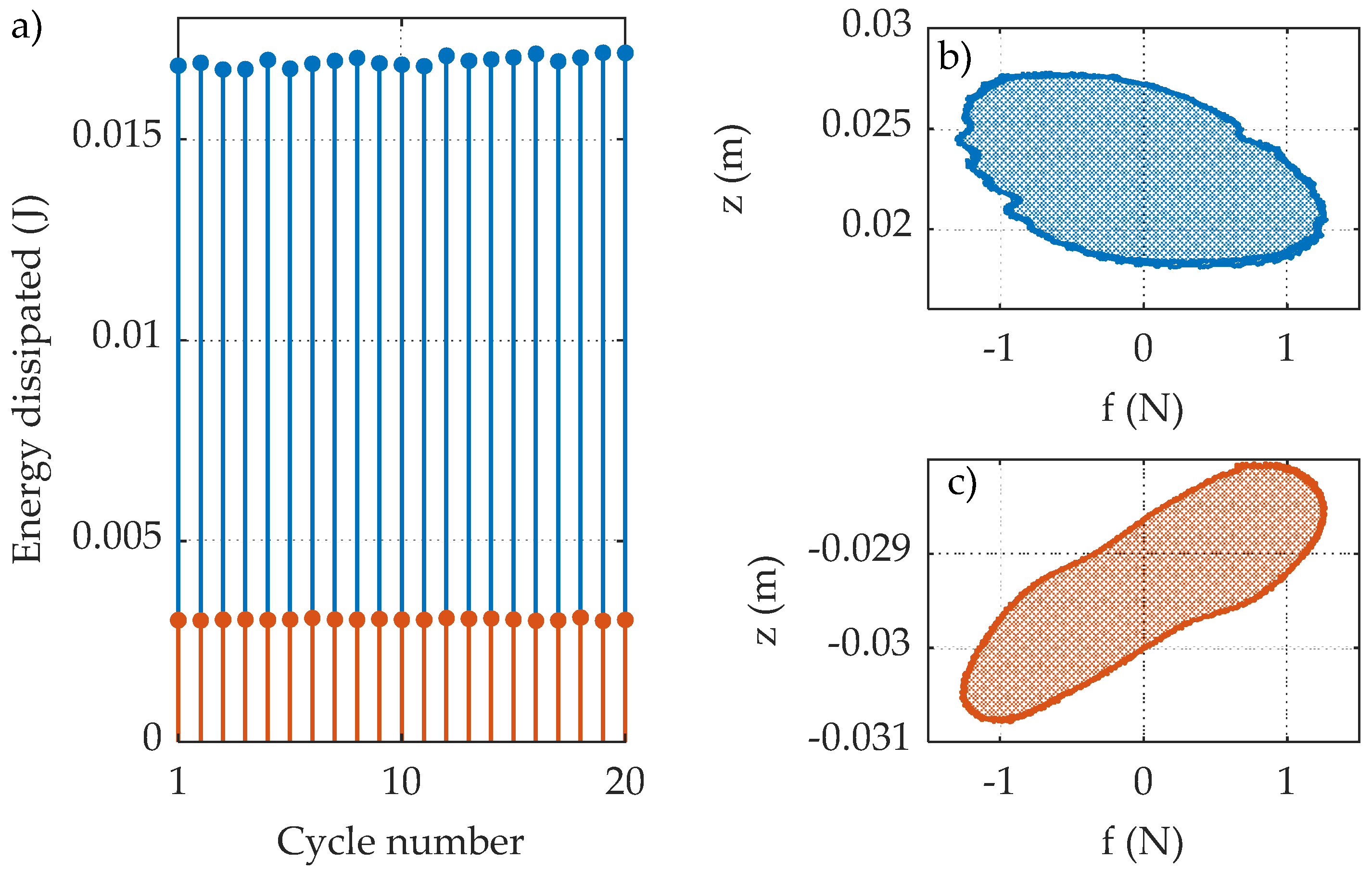
4.1. Experimental Estimation of the Energy Dissipated per Cycle (EDC)

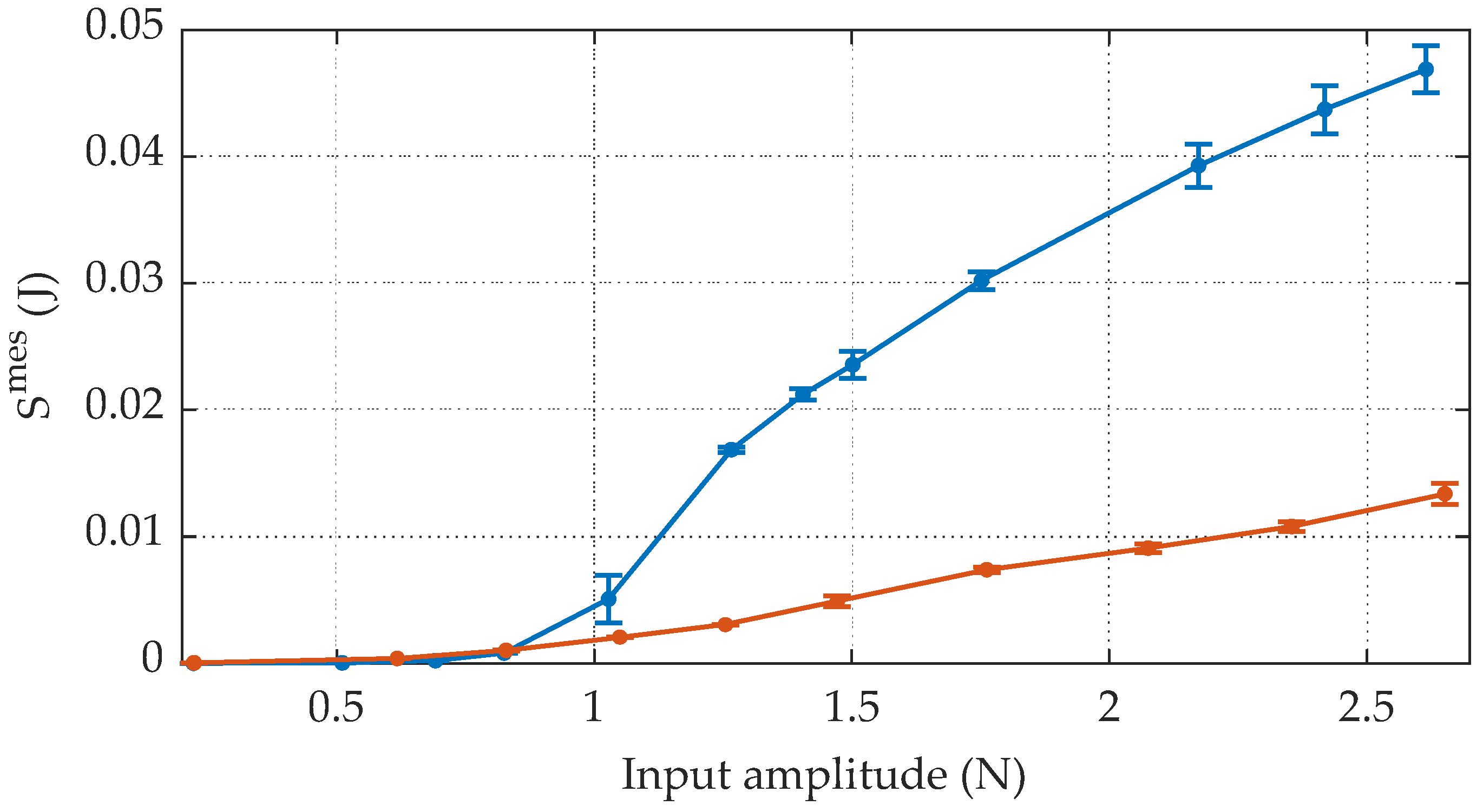
The EDCs are directly estimated from the experimental measurements by numerically computing the integral of the response z ( t ) with respect to the harmonic input f ( t ) for each cycle and averaging over the number of cycles. Transients are removed, so as to take into account only the steady-state responses. Since the measurements are performed starting from the two equilibrium positions, two sets of dissipated energies are collected, called S m e s and S + m e s and refer to the oscillations around z * and z + * , respectively. The complete vector of measured EDCs is therefore S m e s = vec { S m e s , S + m e s } . Each final value S k m e s is obtained by averaging over the cycles, and the associated standard deviation σ k m e s is used as an index of dispersion.
A representative response-input plot is reported in Figure 9 with an excitation amplitude equal to 1.3   N , while Figure 10 depicts the evolution of S m e s with respect to the input amplitudes vector f 0 .
The range of considered input amplitudes goes from 0.2 to 2.7   N . Period doublings start to occur in the experimental measurements beyond this value, which are not the object of this study. The error bars in Figure 10 represent the quantity S k m e s ± 3 σ k m e s .

4.2. Numerical Computation via Harmonic Balance Method with Amplitude Continuation

Considering a harmonic input of the kind f ( t ) = f 0 sin ( ω t ) , the energy dissipated over one cycle S can be written as
S = c y c l e z ( t ) d f = ω f 0 0 2 π ω z ( t ) cos ( ω t ) d t .
Since the system described by Equation (7) is nonlinear, the response z ( t ) to a periodic excitation can be written in terms of a Fourier series with H harmonics:
z ( t ) = Z 0 + Re [ h = 1 H Z h e i h ω t ] .
It can be easily proved that the integral of Equation (11) is zero for each integer harmonic contribution of the response different from 1. Therefore, the EDC reduces to
S = ω f 0 0 2 π ω | Z 1 | sin ( ω t + ϕ 1 ) cos ( ω t ) d t = π f 0 | Z 1 | sin ( ϕ 1 ) ,
where ϕ 1 is the phase of the first harmonic of the response. Note that Equation (13) is valid only if sub-harmonics are not taken into account.
The Fourier coefficients of the response z ( t ) can be rapidly computed via the harmonic balance method for each forcing input amplitude f 0 , k and for a fixed ω . In particular, the focus is to track the evolution of S varying f 0 , and to compare the model predictions S m o d with the experimental observations S m e s of Figure 10. An arc-length continuation procedure (like the one proposed in [30]) is adopted to study the evolution of the dissipated energy. The forcing input amplitude f 0 is therefore chosen as the “continuation parameter” and the solution for each f 0 is sought along the arc-length of a solution branch. This allows to account for possible singularities of the system being Jacobian, which lead to response bifurcations [29]. An illustrative example is exposed in the following.

Illustrative Example

A linear oscillator with continuous velocity-based friction is considered in this example. The system parameters are summarized in Table 2 and the equation of motion reads
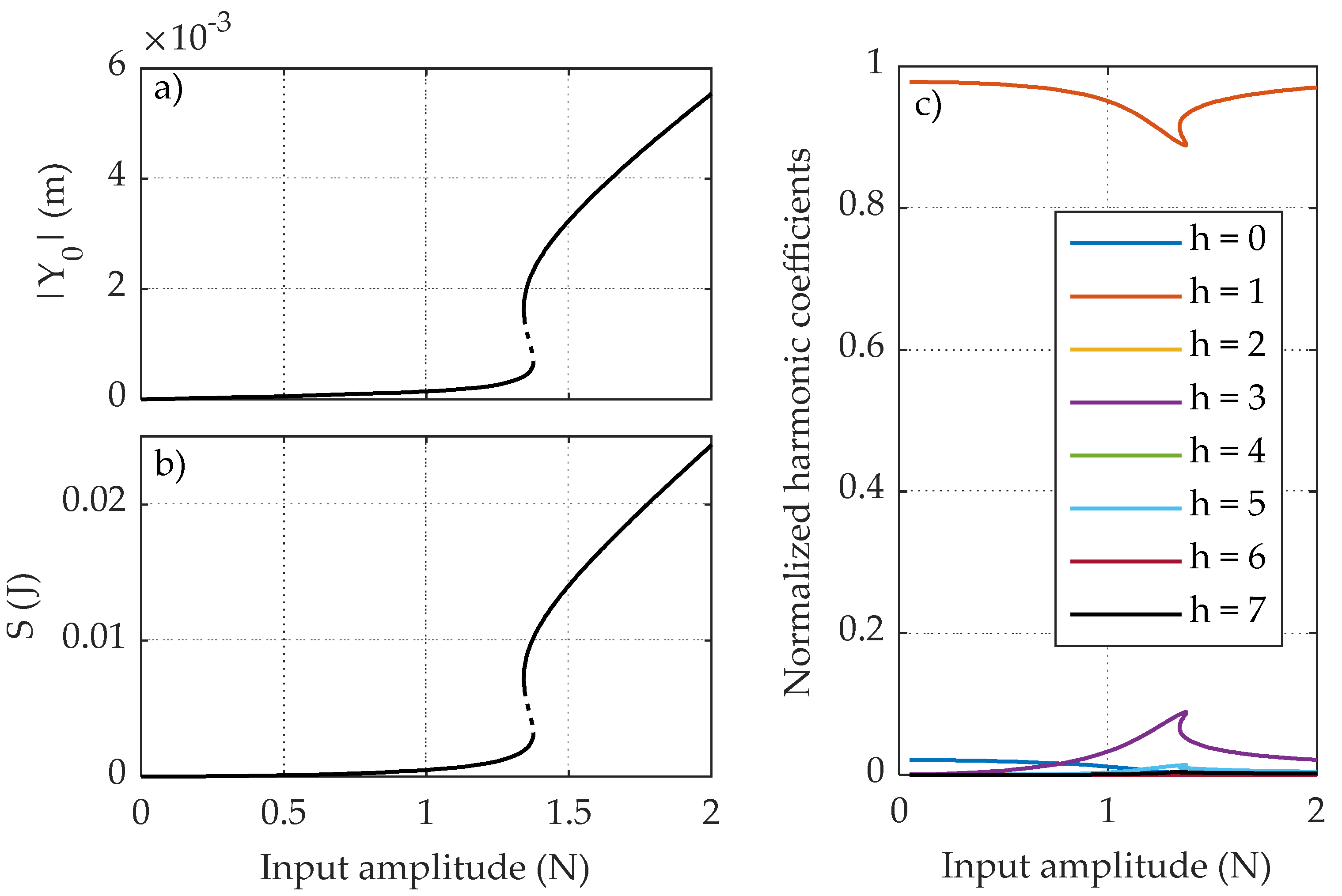
m y ¨ + c y ˙ + k y + f d [ tanh ( 4 y ˙ / v t ) + ( k s 1 ) y ˙ / v t ( 1 4 ( y ˙ / v t ) 2 + 3 4 ) 2 ] = f 0 e i ω t .
The excitation frequency ω is set to 80% of the linear natural frequency of the system k / m   , and the amplitude increases in the range 0 2   N . Seven harmonics are included in the response.
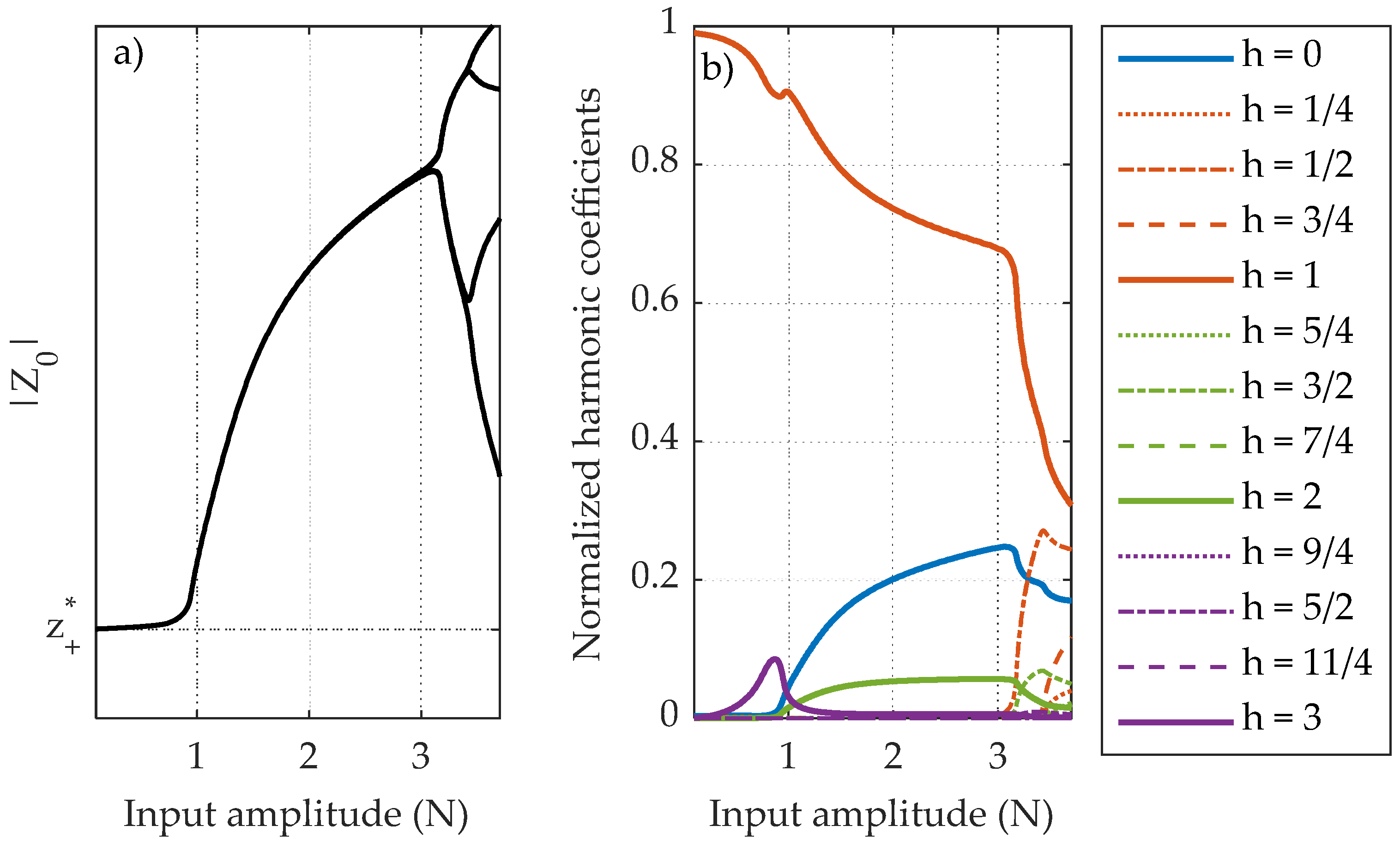
The nonlinear amplitude response curve obtained using HBM with the amplitude continuation is depicted in Figure 11, together with the EDCs and the evolution of the harmonic coefficients. An unstable branch can be noted in the region between 1.3 and 1.4   N . Multiple solutions exist in this region, meaning that the system response would avoid the unstable branch and suddenly reach a new stable solution. This phenomenon is very common in nonlinear systems when sweeping around their resonance frequencies and it is usually called “jump” [29]. Here, the nature of the phenomenon is different, but the behavior is very similar. 
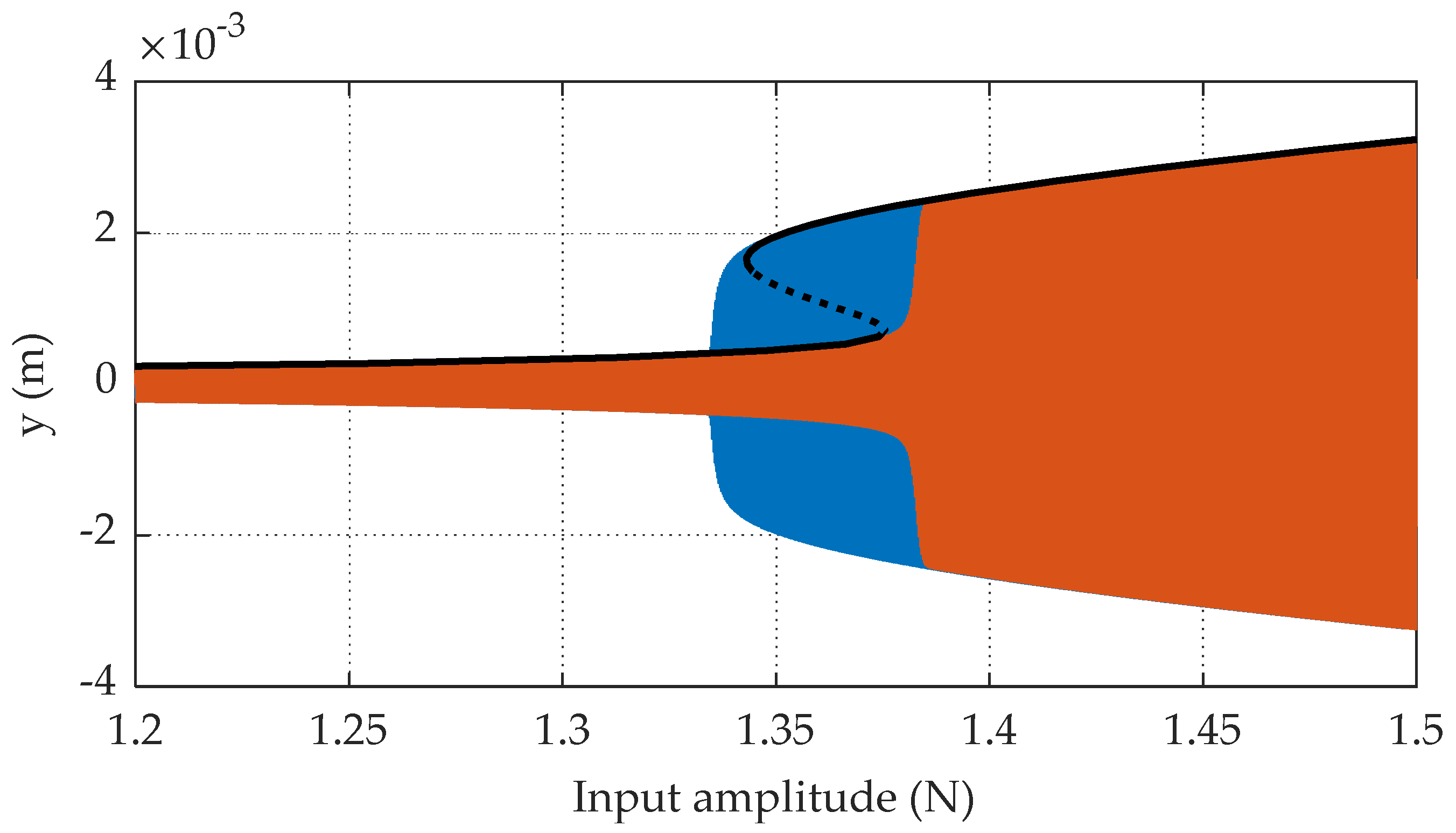
Figure 12 depicts the response of the system around the unstable region computed by numerically integrating the equation of motion with the Newmark algorithm [34] and under the amplitude sweep up and down excitations. The nonlinear amplitude response curve computed with the HBM is also overlapped. The jump phenomenon can be clearly observed. A slight difference can be noted between the HBM and numerical simulations around the jump region. This is probably due to the different kind of excitation in the two approaches: numerical simulations are conducted with an amplitude sweep excitation, which contains transients. The HBM represents instead the steady-state solutions for each input amplitude value.

5. Results and Discussion

The unknown parameters of Equation (7) are identified by optimizing the residuals between the measured EDCs S m e s of Figure 10 and the predicted ones S m o d according to Equation (13). Both sets of measurements around the positive and negative equilibrium positions are considered.
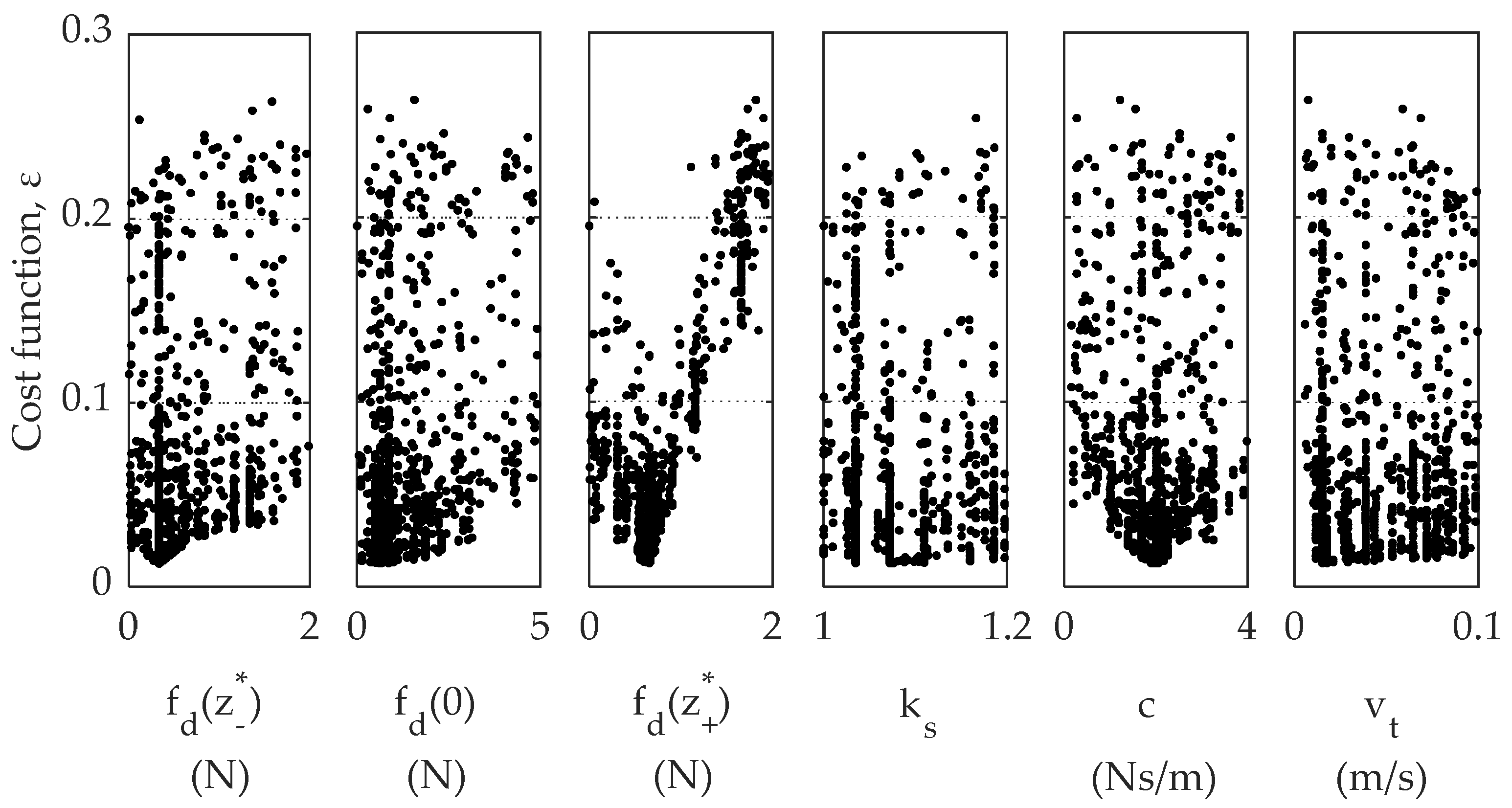
The genetic algorithm is applied considering a population of 100 individuals, 20 generations and 20% mutation rate. The latter in particular is to allow the algorithm to explore a wider range of possible solutions, by randomly modifying a portion of the existing population. The cost function with respect to the single parameters of the optimization is depicted in Figure 13.
It can be noted that the minimum value of the cost function is reached sharply when considering the parameters f d ( z * ) ,   f d ( 0 ) ,   f d ( z + * ) and c , while results are more dispersive for the others. It should be highlighted though that these four parameters have the biggest influence in the EDC of the considered measurements. The transition velocity and the static proportionality coefficient have a major influence in the low-amplitude region, and tend to compensate each other. Some more details are presented in the sensitivity analysis in the next section.
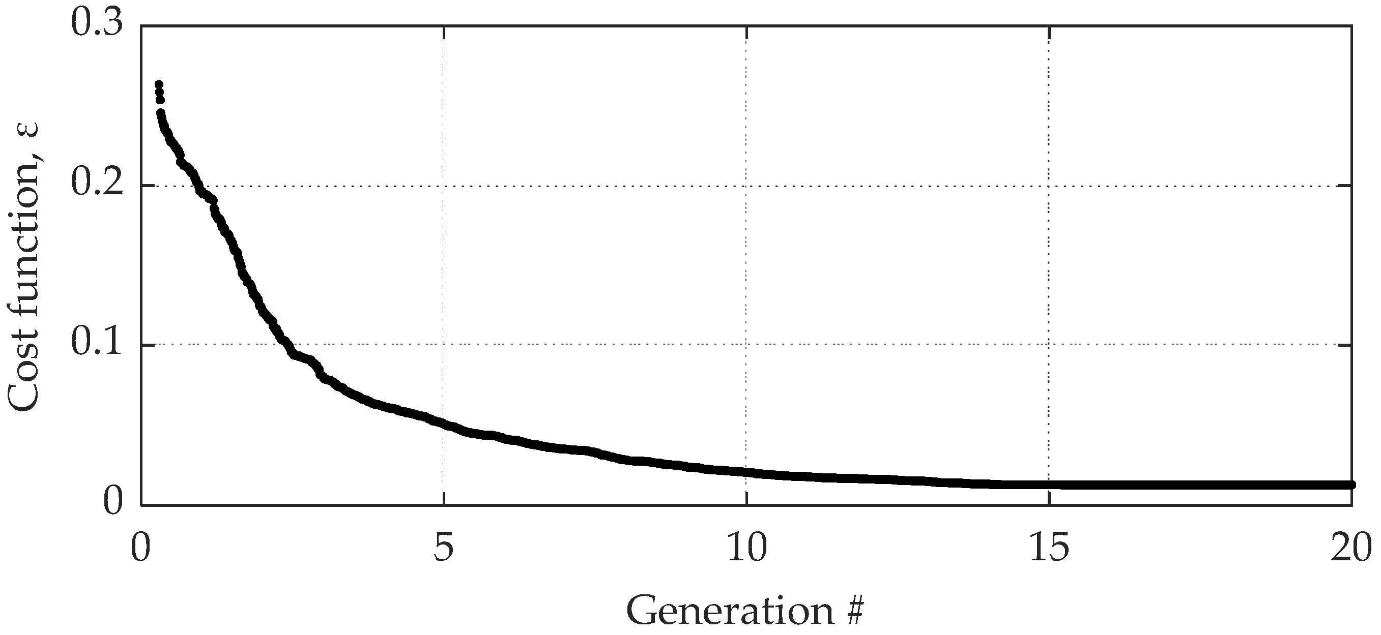
The value of the cost function across the generations of the genetic optimization is reported in Figure 14. The minimum value of the cost function is ε ( θ ¯ ) = 0.012 , and the corresponding set of parameters θ ¯ is listed in Table 3.
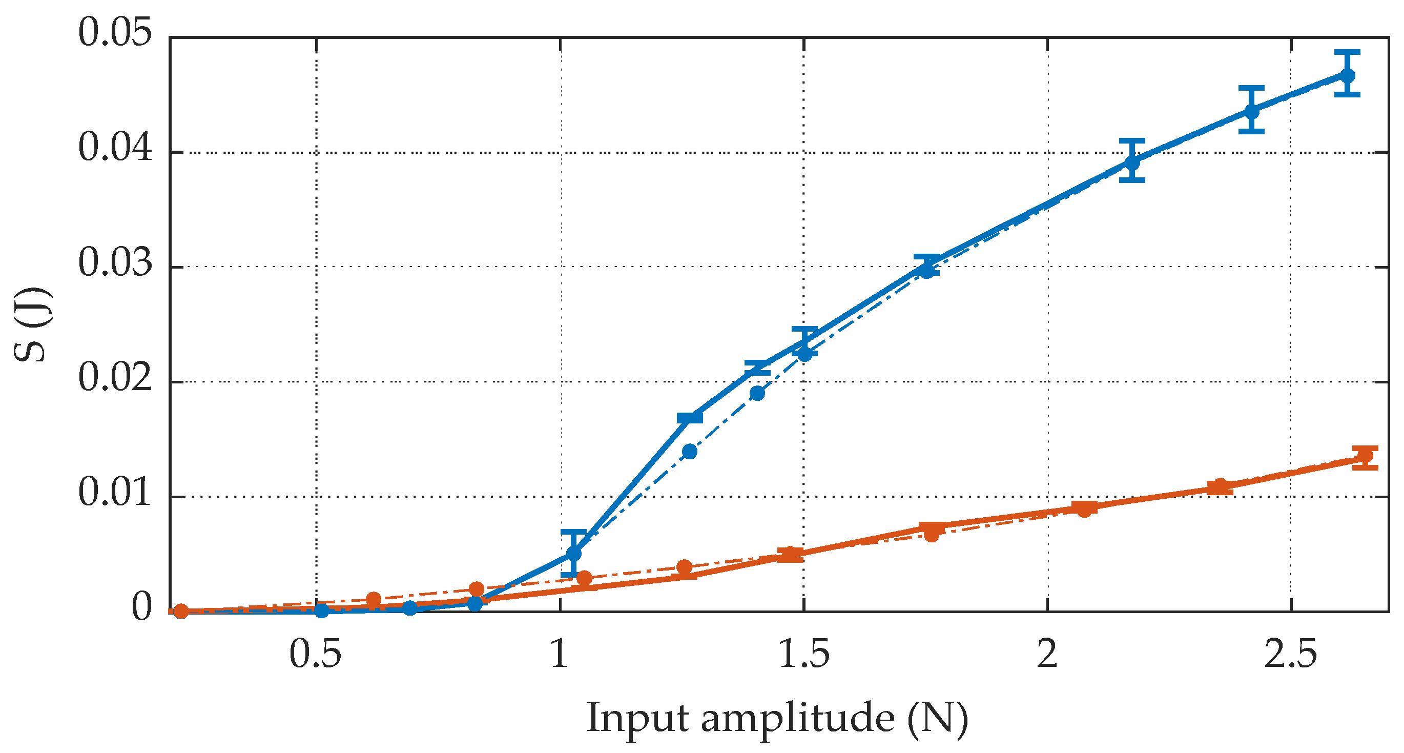
Eventually, the comparison between the measured EDCs and the final model predictions is reported in Figure 15. The average percentage deviation between the measured and predicted EDCs is 6% for the positive oscillations and 12% for the negative ones. The model nicely captures the nonlinear dynamics of the system, especially at higher input amplitudes. Errors are instead more consistent in the low-amplitude region. Nevertheless, displacements in this region are so small that other phenomena might be involved, such as displacement-dependent and hysteretic frictional behavior.

5.1. Sensitivity Analysis

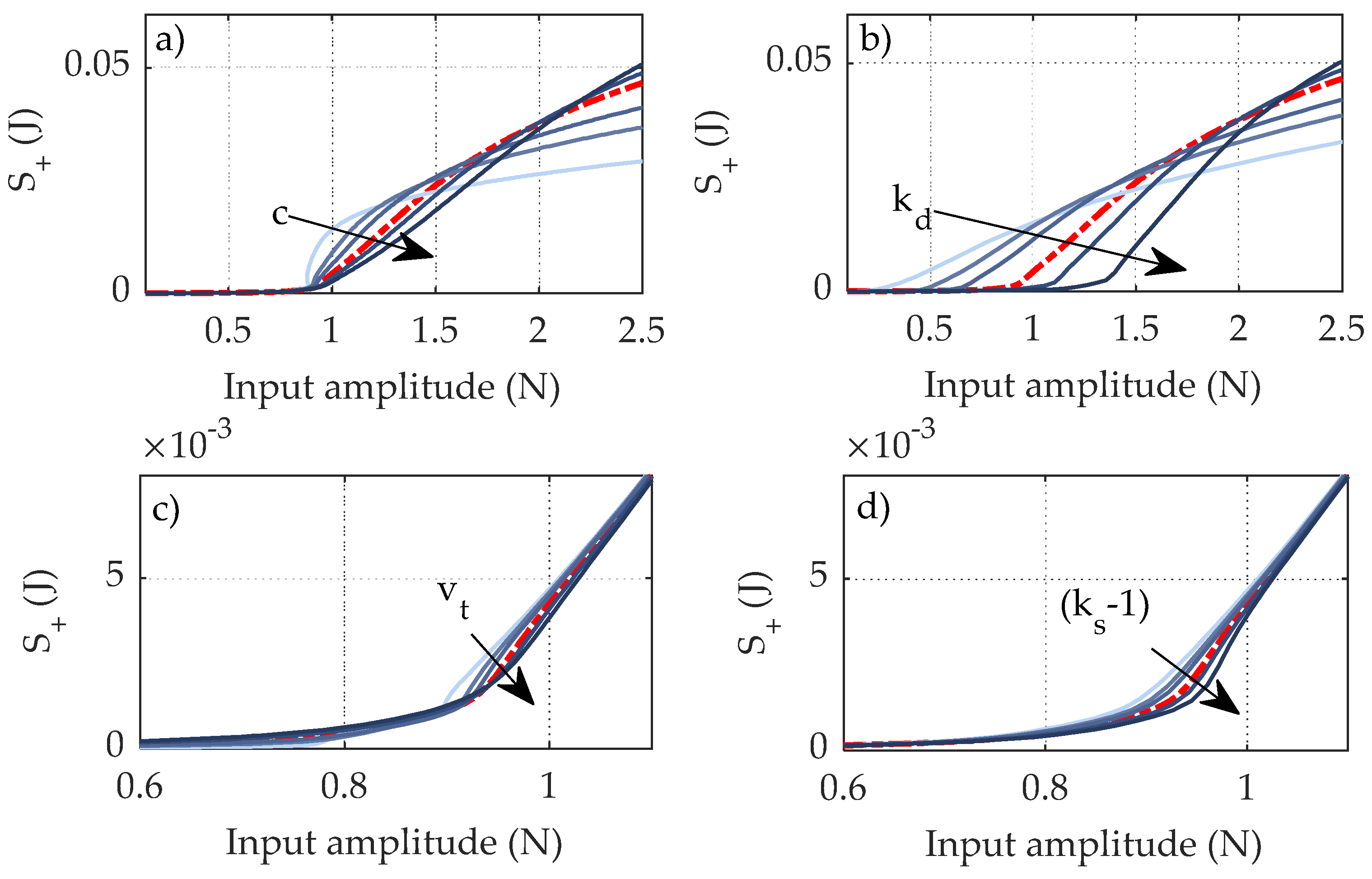
A sensitivity analysis is carried out on the parameters of the identification to check their influence on the predicted EDCs. The parameters are varied in the measure of 20%, 50%, 70%, 120% and 150% of their identified values in Table 3. In particular, f d ( z ) is varied with a coefficient k d , so as to consider the quantity k d f d ( z ) . Figure 16 shows the results of the sensitivity analysis on the EDCs associated with the oscillations around the positive equilibrium position.
As expected, the linear viscous damping and the dynamic friction term have the highest influence on the overall behavior of the EDC. The transition velocity and the static friction term have some importance in the low-amplitude area. Given the poor number of experimental points in this region, their effects are difficult to separate in the optimization process, thus explaining their dispersion in Figure 13. Furthermore, low-amplitude oscillations might be affected by other phenomena, such as hysteresis loops, which are not considered in this study.

5.2. Nonlinear Amplitude Response Curves

Finally, the identified model is used to build the nonlinear amplitude response curve of the structure, with an excitation frequency ν = 9   Hz and an input amplitude range of 0.1 3.7   N . As already pointed out in Section 4.1, period doublings start to occur in the experimental measurements after 2.7   N . For this reason, sub-harmonics up to 1 / 4 ν are also included in the following test to check whether this happens also in the model. Figure 17 depicts the nonlinear amplitude response curve starting from the positive equilibrium position, as well as the normalized harmonic coefficients. It can be noted that sub-harmonics start to show up around the 3   N input amplitude, resulting in a period-doubling cascade. Representations like the one in Figure 17a are usually called “bifurcation maps”. Each point of a bifurcation map represents the amplitude(s) of the steady-state solution for a specific value of the excitation amplitude. However, the map in Figure 17a is built using the harmonic balance method, which allows only a certain number of sub/super-harmonics to be considered in the response. In other words, it is not possible to predict chaotic behavior with this tool, as a periodic response is needed.
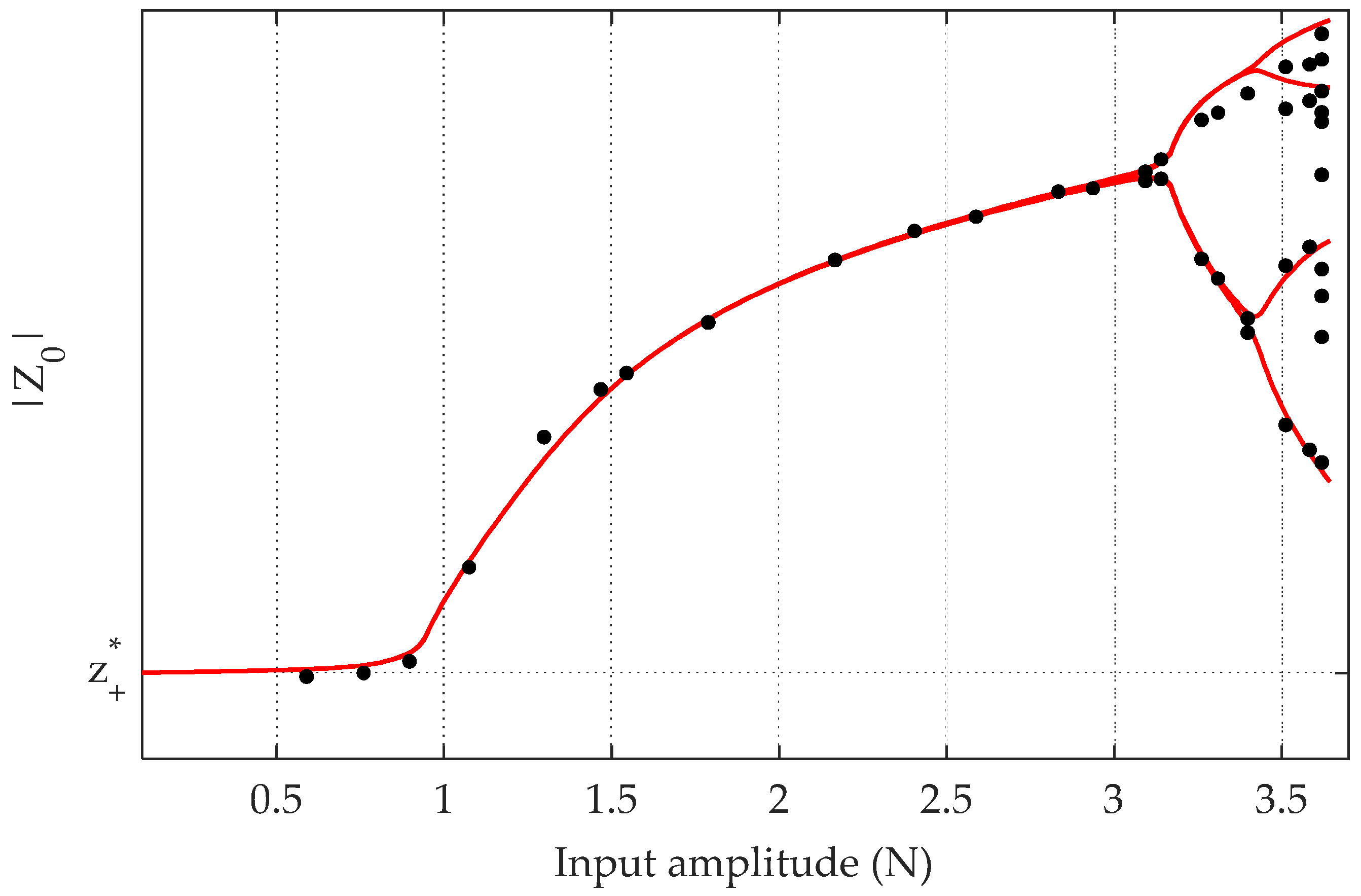
A final validation of the goodness of the model is depicted in Figure 18, showing the experimental bifurcation map compared with the predicted one. The deviations between the predictions and observations resemble the ones obtained with the EDCs in the amplitude range up to 2.7 N. Higher discrepancies show up after period doublings start to appear. This is somehow expected, since the model has been trained on lower amplitudes. Further, period doublings are difficult to handle experimentally, as the system starts to show a considerable dependence on small external perturbations, such as noise. This makes the amplitudes of the periodic solutions to be quite variable, and the forcing input difficult to control.
The encouraging results prove the goodness of the presented methodology and provide a reliable model for a system with rich and strong nonlinear dynamics.

6. Conclusions

In this paper, the nonlinear identification of a negative stiffness oscillator has been presented. In particular, the damping force of the device has been identified upon a physically based model, governed by a frictional behavior and dependent on the velocity and position. The identification has been carried out by minimizing the residuals between the model predictions and experimental observations. In particular, the energy dissipated per cycle has been adopted as the optimization criterion. On the experimental side, the system has been driven through harmonic tests with several input amplitudes, in order to estimate the variations in the energy dissipated per cycle. On the computational side, the harmonic balance method has been implemented with a continuation technique on the forcing input amplitudes. Results show a good confidence in the identified parameters, with low residuals in the analyzed input amplitude range. This confirm the effectiveness of the presented methodology, which can be applied to a wide class of nonlinear systems.

Author Contributions

Methodology, D.A.; Supervision, S.M.; Writing—original draft, D.A. All authors have read and agreed to the published version of the manuscript

Funding

This research received no external funding.

Conflicts of Interest

The authors declare no conflict of interest.

References

  1. Worden, K.; Wong, C.X.; Parlitz, U.; Hornstein, A.; Engster, D.; Tjahjowidodo, T.; Al-Bender, F.; Rizos, D.D.; Fassois, S.D. Identification of pre-sliding and sliding friction dynamics: Grey box and black-box models. Mech. Syst. Signal Process. 2007, 21, 514–534. [Google Scholar] [CrossRef]
  2. Berger, E.J. Friction modeling for dynamic system simulation. Appl. Mech. Rev. 2002, 55, 535–577. [Google Scholar] [CrossRef] [Green Version]
  3. Armstrong-Hélouvry, B.; Dupont, P.; De Wit, C.C. A survey of models, analysis tools and compensation methods for the control of machines with friction. Automatica 1994, 30, 1083–1138. [Google Scholar] [CrossRef]
  4. Swevers, J.; Al-Bender, F.; Ganseman, C.G.; Prajogo, T. An integrated friction model structure with improved presliding behavior for accurate friction compensation. IEEE Trans. Automat. Contr. 2000, 45, 675–686. [Google Scholar] [CrossRef]
  5. Al-Bender, F. Fundamentals of friction modeling. Proc. ASPE Spring Top. Meet. Control Precis. Syst. (ASPE 2010). 2010, 48, 117–122. [Google Scholar]
  6. Coulomb, C.A. Théorie des Machines Simples, en Ayant Égard au Frottement de Leurs Parties, et a la Roideur des Cordages, Nouv. éd., à Laquelle on a Ajouté les Mémoires du Même Auteur; Bachelier: Paris, France, 1821. [Google Scholar]
  7. Kerschen, G.; Worden, K.; Vakakis, A.F.; Golinval, J.C. Past, present and future of nonlinear system identification in structural dynamics. Mech. Syst. Signal Process. 2006, 20, 505–592. [Google Scholar] [CrossRef] [Green Version]
  8. Noël, J.P.; Kerschen, G. Nonlinear system identification in structural dynamics: 10 more years of progress. Mech. Syst. Signal Process. 2017, 83, 2–35. [Google Scholar] [CrossRef]
  9. Rizos, D.D.; Fassois, S.D. Friction identification based upon the LuGre and Maxwell slip models. IFAC Proc. Vol. 2005, 38, 548–553. [Google Scholar] [CrossRef]
  10. De Wit, C.C.; Lischinsky, P.; Åström, K.J.; Olsson, H. A new model for control of systems with friction. IEEE Trans. Automat. Contr. 1995, 40, 419–425. [Google Scholar] [CrossRef] [Green Version]
  11. Lampaert, V.; Swevers, J.; Al-Bender, F. Modification of the Leuven integrated friction model structure. IEEE Trans. Automat. Contr. 2002, 47, 683–687. [Google Scholar] [CrossRef] [Green Version]
  12. Wang, X.; Lin, S.; Wang, S. Dynamic friction parameter identification method with LuGre model for Direct-Drive Rotary torque motor. Math. Probl. Eng. 2016, 2016. [Google Scholar] [CrossRef] [Green Version]
  13. Noël, J.P.; Esfahani, A.F.; Kerschen, G.; Schoukens, J. A nonlinear state-space approach to hysteresis identification. Mech. Syst. Signal Process. 2017, 84, 171–184. [Google Scholar] [CrossRef] [Green Version]
  14. Dossogne, T.; Noël, J.P.; Grappasonni, C.; Kerschen, G.; Peeters, B.; Debille, J.; Vaes, M.; Schoukens, J. Nonlinear ground vibration identification of an F-16 aircraft-Part II: Understanding nonlinear behaviour in aerospace structures using sine-sweep testing. In Proceedings of the International Forum on Aeroelasticity and Structural Dynamics (IFASD 2015), Saint Petersburg, Russia, 28 June–2 Juny 2015; pp. 1–19. [Google Scholar]
  15. Masri, S.F.; Caughey, T.K. A nonparametric identification technique for nonlinear dynamic problems. J. Appl. Mech. Trans. ASME 1979, 46, 433–447. [Google Scholar] [CrossRef]
  16. Worden, K.; Tomlinson, G.R. Nonlinearity in Structural Dynamics; CRC Press: Boca Raton, FL, USA, 2019; ISBN 9780429138331. [Google Scholar]
  17. Petrov, E.P.; Ewins, D.J. Analytical formulation of friction interface elements for analysis of nonlinear multi-harmonic vibrations of bladed disks. J. Turbomach. 2003, 125, 364–371. [Google Scholar] [CrossRef]
  18. Maria, C.; Zucca, S. Modelling friction contacts in structural dynamics and its application to turbine bladed disks. Numer. Anal. Theory Appl. 2011. [Google Scholar] [CrossRef] [Green Version]
  19. Charleux, D.; Gibert, C.; Thouverez, F.; Dupeux, J. Numerical and experimental study of friction damping blade attachments of rotating bladed disks. Int. J. Rotating Mach. 2006, 2006, 1–13. [Google Scholar] [CrossRef] [Green Version]
  20. Claeys, M.; Sinou, J.J.; Lambelin, J.P.; Todeschini, R. Modal interactions due to friction in the nonlinear vibration response of the “Harmony” test structure: Experiments and simulations. J. Sound Vib. 2016, 376, 131–148. [Google Scholar] [CrossRef]
  21. Ahmadian, H.; Jalali, H.; Pourahmadian, F. Nonlinear model identification of a frictional contact support. Mech. Syst. Signal Process. 2010, 24, 2844–2854. [Google Scholar] [CrossRef]
  22. Sorrentino, S.; Anastasio, D.; Fasana, A.; Marchesiello, S. Distributed parameter and finite element models for wave propagation in railway contact lines. J. Sound Vib. 2017, 410, 1–18. [Google Scholar] [CrossRef]
  23. Anastasio, D.; Fasana, A.; Garibaldi, L.; Marchesiello, S. Analytical investigation of railway overhead contact wire dynamics and comparison with experimental results. Mech. Syst. Signal Process. 2019, 116, 277–292. [Google Scholar] [CrossRef]
  24. Jordan, D.; Smith, P. Nonlinear Ordinary Differential Equations: An Introduction for Scientists and Engineers; Oxford University Press: Oxford, UK, 2007; ISBN 0199208255. [Google Scholar]
  25. Moon, F.C.; Holmes, P.J. A magnetoelastic strange attractor. J. Sound Vib. 1979, 65, 275–296. [Google Scholar] [CrossRef]
  26. Kovacic, I.; Brennan, M.J. The Duffing Equation: Nonlinear Oscillators and their Behaviour; Kovacic, I., Brennan, M.J., Eds.; John Wiley & Sons, Ltd: Chichester, UK, 2011; ISBN 9780470715499. [Google Scholar]
  27. Anastasio, D.; Fasana, A.; Garibaldi, L.; Marchesiello, S. Nonlinear dynamics of a duffing-like negative stiffness oscillator: Modeling and experimental characterization. Shock Vib. 2020, 2020, 1–13. [Google Scholar] [CrossRef]
  28. Marchesiello, S.; Garibaldi, L. A time domain approach for identifying nonlinear vibrating structures by subspace methods. Mech. Syst. Signal Process. 2008, 22, 81–101. [Google Scholar] [CrossRef]
  29. Detroux, T.; Renson, L.; Masset, L.; Kerschen, G. The harmonic balance method for bifurcation analysis of large-scale nonlinear mechanical systems. Comput. Methods Appl. Mech. Eng. 2015, 296, 18–38. [Google Scholar] [CrossRef] [Green Version]
  30. Von Groll, G.; Ewins, D.J. The harmonic balance method with arc-length continuation in rotor/stator contact problems. J. Sound Vib. 2001, 241, 223–233. [Google Scholar] [CrossRef] [Green Version]
  31. Xie, L.; Baguet, S.; Prabel, B.; Dufour, R. Bifurcation tracking by harmonic balance method for performance tuning of nonlinear dynamical systems. Mech. Syst. Signal Process. 2017, 88, 445–461. [Google Scholar] [CrossRef] [Green Version]
  32. Deb, K. Multi-Objective Optimization Using Evolutionary Algorithms; John Wiley & Sons, Inc.: Chichester, UK, 2001; ISBN 978-0-471-87339-6. [Google Scholar]
  33. Brown, P.; McPhee, J. A continuous velocity-based friction model for dynamics and control with physically meaningful parameters. J. Comput. Nonlinear Dyn. 2016, 11, 1–6. [Google Scholar] [CrossRef]
  34. Newmark, N.M. A method of computation for structural dynamics. J. Eng. Mech. Div. 1959, 85, 1235–1264. [Google Scholar]
Figure 1. Schematic representation of the negative stiffness oscillator.
Vibration 03 00011 g001
Figure 2. Qualitative representation of the potential U ( z ) . Red dots: equilibrium positions.
Vibration 03 00011 g002
Figure 3. Photos of the experimental setup. (a) Negative equilibrium position z * ; (b) positive equilibrium position z + * .
Vibration 03 00011 g003
Figure 4. Measured cross-well oscillations under random excitation in [27].
Vibration 03 00011 g004
Figure 5. Experimental restoring surface from [27] with cross-well random excitation in (a); experimental restoring force (blue dots, ϵ s = 0.1 % and identified restoring force (red line) in (b); experimental damping forces around z * (green dots, ϵ d = 0.1 % ) and z + * (yellow dots, ϵ d = 0.1 % ) in (c).
Vibration 03 00011 g005
Figure 6. Stepped sine tests. Oscillations around the positive equilibrium in (a) and around the negative equilibrium in (b).
Vibration 03 00011 g006
Figure 7. Experimental restoring surface with stepped sine excitations in (a); experimental restoring force (blue dots, ϵs = 0.1%) and identified restoring force (red line) in (b); experimental damping forces around z * (green dots, ϵ d = 0.1 % ) and z + * (yellow dots, ϵ d = 0.1 % ) in (c).
Vibration 03 00011 g007
Figure 8. Variation in the experimental damping force across the position of the moving mass, | z z ˜ | < ϵ d with ϵ d = 0.1 % .
Vibration 03 00011 g008
Figure 9. Energy dissipated per cycle in (a) with excitation amplitude of 1.3 N. Blue: oscillations around the positive equilibrium position; orange: oscillations around the negative equilibrium position. Corresponding response-input plots in (b) and (c) with highlighted areas.
Vibration 03 00011 g009
Figure 10. Experimental estimation of the dissipated energy per cycle. Blue line: oscillations around z + * ; orange line: oscillations around z * . Bars represent the quantity S k m e s ± 3 σ k m e s .
Vibration 03 00011 g010
Figure 11. Harmonic balance method (HBM) with amplitude continuation, illustrative example. Dashed lines represent unstable paths. Response amplitude in (a); energy dissipated per cycle (EDC) in (b); normalized harmonic coefficients in (c).
Vibration 03 00011 g011
Figure 12. Comparison between the HBM and numerical integration, illustrative example. Blue line: numerical integration with amplitude sweep down sine excitation; orange line: numerical integration with amplitude sweep up sine excitation; black line: the HBM with amplitude continuation.
Vibration 03 00011 g012
Figure 13. Cost function ε with respect to the parameters of the optimization.
Vibration 03 00011 g013
Figure 14. Cost function ε across the generations.
Vibration 03 00011 g014
Figure 15. Energy dissipated per cycle. Continuous lines: experimental estimations S m e s ± 3 σ m e s ; dashed-dotted lines: final model predictions. Blue line: oscillations around z + * ; orange line: oscillations around z * .
Vibration 03 00011 g015
Figure 16. Sensitivity analysis on the parameters of the identification. Dashed-dotted red line: reference EDC with the identified values. Blue lines: EDCs corresponding to a 20%, 50%, 70%, 120% and 150% variation of the selected parameter.
Vibration 03 00011 g016
Figure 17. The HBM with amplitude continuation, final model. Response amplitude in (a); normalized harmonic coefficients in (b).
Vibration 03 00011 g017
Figure 18. Bifurcation map of the system in the range 0.1–3.7 N. Black dots: experimental observations; red line: nonlinear amplitude response curve with the HBM.
Vibration 03 00011 g018
Table 1. Previously identified coefficients of the restoring force.
k3 (N/m3)k2 (N/m2)k1 (N/m)k0 (N)
7.35 · 1051.56 · 1035502.4
Table 2. Parameters of the illustrative example.
m   ( k g ) k   ( N / m ) c   ( N s / m ) f d   ( N ) k s v t   ( m / s )
1.3800111.210−2
Table 3. Identified values.
f d ( z * ) ( N )   f d ( 0 )   ( N ) f d ( z + * )   ( N )   k s   c   ( N s / m )   v t   ( m / s )  
0.33 0.67 0.66 1.07 2.02 1.5 10 2

