An Optimization-Based Framework for Nonlinear Model Selection and Identification

Abstract

This paper proposes an optimization-based framework to determine the type of nonlinear model present and identify its parameters. The objective in this optimization problem is to identify the parameters of a nonlinear model by minimizing the differences between the experimental and analytical responses at the measured coordinates of the nonlinear structure. The application of the method is demonstrated on a clamped beam subjected to a nonlinear electromagnetic force. In the proposed method, the assumption is that the form of nonlinear force is not known. For this reason, one may assume that any nonlinear force can be described using a Taylor series expansion. In this paper, four different possible nonlinear forms are assumed to model the electromagnetic force. The parameters of these four nonlinear models are identified from experimental data obtained from a series of stepped-sine vibration tests with constant acceleration base excitation. It is found that a nonlinear model consisting of linear damping and linear, quadratic, cubic, and fifth order stiffness provides excellent agreement between the predicted responses and the corresponding measured responses. It is also shown that adding a quadratic nonlinear damping does not lead to a significant improvement in the results.

1. Introduction

Mathematical models have been increasingly used in nonlinear structural dynamics. However, the type of nonlinearity and the parameters of these nonlinear models need to be identified from experimental data. This is mainly due to the lack of knowledge about the mechanism of the nonlinearity in structures while in service. Therefore, there has been considerable interest in nonlinear model identification using vibration test data. Thus the identified mathematical model should not only be capable of predicting the real-life behavior of an unknown structure, but also must be physically meaningful. In other words, it is essential to ensure that any mathematical model developed through the process of identification is a valid physical model. Having a valid physical model in the identification process using experimental data will lead to more reliable and meaningful identified parameters.

Recently, various identification methods have been introduced to identify linear and nonlinear structures, [1,2,3,4,5,6]. References [5,6] have reviewed past and recent studies focusing on the methods introduced for identifying the nonlinear systems. These methods can be categorized according to different criteria. First is the type of data required for identification; whether the measured data is used in the time domain [7,8,9,10], frequency domain [11,12,13,14,15,16,17,18,19,20,21,22], or both [23,24,25]. The second is whether the measured degrees of freedom are spatially complete or incomplete. The necessity of knowing or assuming the type of nonlinearity a priori is required for some methods [10,12,20], while some others do not require pre-knowledge (or assumptions) of the type of nonlinearity [21,22].

One deficiency in using the conventional methods, such as $H_1$ and $H_2$, to estimate the frequency response functions of nonlinear systems is that such methods are not able to eliminate the effect of nonlinearities in the system and subsequently predict the underlying linear system accurately. To solve this problem, Richards and Singh [11] presented a spectral identification method based on the “reverse path” formulation to identify multi-degree of freedom nonlinear systems using multi-input multi-output data. For this purpose, broad-band Gaussian random excitation is applied to obtain the nonlinear response of the system. In this approach, the nonlinear elements are considered as feedback forces on the underlying linear system. The application of this method can be found in References [12,13,14,15,26]. Kerschen and Golinval [14] utilized the aforementioned method to introduce a two-step identification approach to generate accurate finite element models of nonlinear structures. In their proposed approach, frequency response functions of the underlying linear system resulting from the Conditioned Reverse Path (CRP) method are correlated with the analytical FRFs to update the linear parameters of the system. CRP was used in [12] to identify and investigate the behavior of a cantilever beam with a geometric nonlinearity. Lenaerts et al. [10] used the updating technique of proper orthogonal decomposition to study the test system of the companion paper [12].

Noël and Kerschen [16] introduced a frequency-domain method to identify nonlinear systems. In this subspace-based technique, the nonlinearity of the system is considered as a feedback force applied to the underlying linear system and is identified utilizing the frequency domain data. Noël et al. [23] investigated a nonlinear spacecraft using two subspace methods in both time and frequency domains. Using these methods, they exploited periodic random measurements to identify the modal parameters of the underlying linear system and the parameters of nonlinear elements of the system.

Hill et al. [17] studied the behavior of a two-degree-of-freedom system subjected to an external force utilizing the backbone curves of the system. They presented a method to find the backbone curves of the system using the second order normal form technique. Renson et al. [18] developed a method to extract the backbone curve of the underlying conservative system. They adapted control-based continuation to track the locus where the response and the excitation are in quadrature. Londoño et al. [19] introduced a method to identify systems with discrete nonlinearities by exciting the structure at a single resonant frequency making the structure vibrate with large displacement where significant effects of nonlinearities are assured. In this method, assuming a form of nonlinearity, the system backbone curves are used to identify the linear and nonlinear parameters of the system. The backbone curves are estimated using measured decay data.

Having measured input data is an important part of conventional identification methods. In order to ignore the necessity of input data measurement, Haroon et al. [24] took advantage of both time and frequency domain techniques to present an approach for identifying the nonlinear elements of structures in the absence of measured input data. Time domain data is used to find a proper assumption for the form of nonlinearity, and the assumed nonlinear form is used with frequency domain data to find an appropriate model to predict the linear and nonlinear response of the system.

This paper proposes a framework using an optimization-based method for nonlinear system identification. The method assumes that the nonlinear force can be expanded using a Taylor series. This mathematical model consists of a linear part (first order term) that can be identified from well-known sensitivity-based model updating [2,3,4] and, for the nonlinear part, the order of the nonlinearity increases sequentially, and optimization-based method can be used to identify the parameters for each case. The proposed method is applied to a cantilever beam subjected to an electromagnetic force. The whole system is base excited, and thus a cantilever beam is clamped to the movable bed of a shaker. Two permanent magnets attached to both sides of the tip of the beam along with two electromagnets located symmetrically on the two sides of the permanent magnets generate the nonlinear restoring force applied on the beam. The structure is excited by constant acceleration base motion of the shaker. First, the underlying linear system is updated using the linear response of the system obtained from low amplitude excitation. Afterwards, the nonlinear frequency response of the system measured from a high amplitude vibration test is used to estimate the coefficients of the possible models for nonlinear electromagnetic force.

2. Experimental Set-Up

A cantilever steel beam of length $30\mathrm{cm}$, width $3\mathrm{cm}$, thickness $1.5\mathrm{mm}$, density $7800\mathrm{kg}/{\mathrm{m}}^3$, and modulus of elasticity $193\mathrm{GPa}$, is considered in this study. The beam is clamped to the movable shaker bed and is subject to constant acceleration base excitation using a stepped-sine test. A nonlinear electromagnetic restoring force is applied to the tip of the cantilever beam. This nonlinear force is generated by a pair of permanent magnets attached to the tip of the beam and a pair of electromagnets mounted on a movable shaker bed on both sides of the permanent magnets. The properties of the permanent magnets and the electromagnets are given in

Table 1. The properties of the permanent magnets and electromagnets used in experimental study.

Parameters	Values
Mass of each permanent magnet	4 g
Strength of permanent magnets	(N42 Neodymium magnets) with 2 kg pull strength
Electromagnets	25 kg pull strength
Input voltage of electromagnets	20 V
Distance of electromagnets from permanent magnets at beam equilibrium position	6 cm
Electromagnetic force direction	Attractive

. There is a gap of $6\mathrm{cm}$ between the permanent and electro magnets at the rest position of the beam. A voltage level of $20\mathrm{V}$ is applied to the two electromagnets to create attractive magnetic forces. One accelerometer is used to measure the movement of the shaker table. Three accelerometers, labelled AM1, AM2, and AM3, with masses of $8\mathrm{g}$ each are attached to the beam, respectively, at distances $5,15,$ and $25\mathrm{cm}$ from the clamped end, to measure the translational acceleration of the beam. 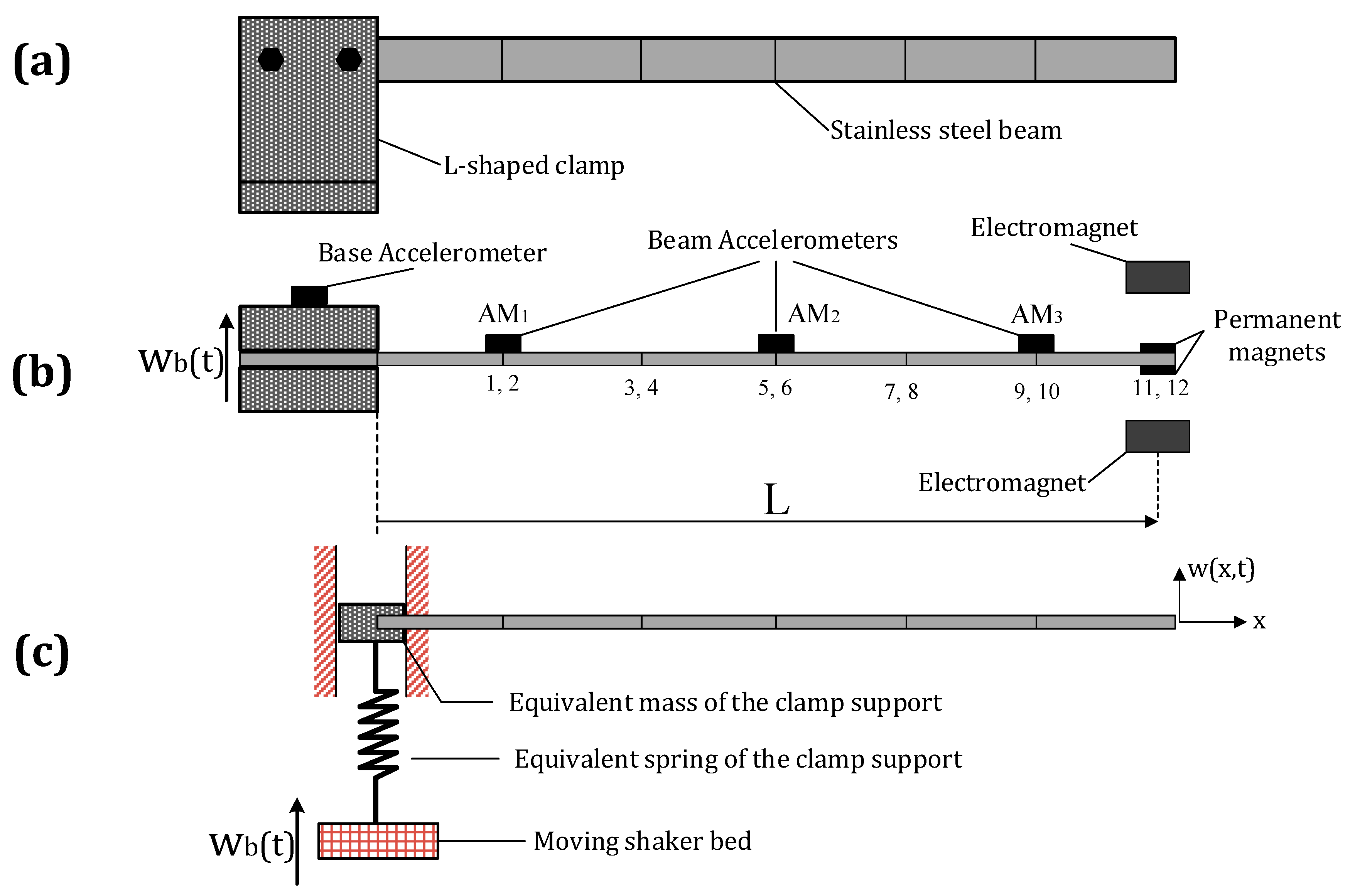Figure 1 shows the experimental set-up and its schematic. $w_b\left(t\right)$ in Figure 1 denotes the base motion of the shaker bed in the direction of the transverse vibration of the beam.

As explained later in this paper, two types of tests are required in the identification process of the present study; first a low amplitude test to measure the linear response of the system is utilized to update the underlying linear model, and second a high amplitude test to measure the nonlinear response of the system is used in the identification process. For the low amplitude test, the structure is excited by a constant acceleration excitation of amplitude $0.02\mathrm{g}$, where $\mathrm{g}$ is the gravitational acceleration. Figure 2 illustrates the linear response of the structure excited by low amplitude base motion with a constant acceleration of 0.02 g. $A_1$, $A_2$, and $A_3$ denote the accelerations measured by accelerometers AM1, AM2, and AM3, respectively. In order to obtain a nonlinear response from the high amplitude test, the amplitude of the excitation has to be large enough to guarantee that the nonlinearity of the system is excited. In this study, the base of the structure (shaker bed) is excited by a constant acceleration of amplitude $0.08\mathrm{g}$ to assure the nonlinear response of the system.

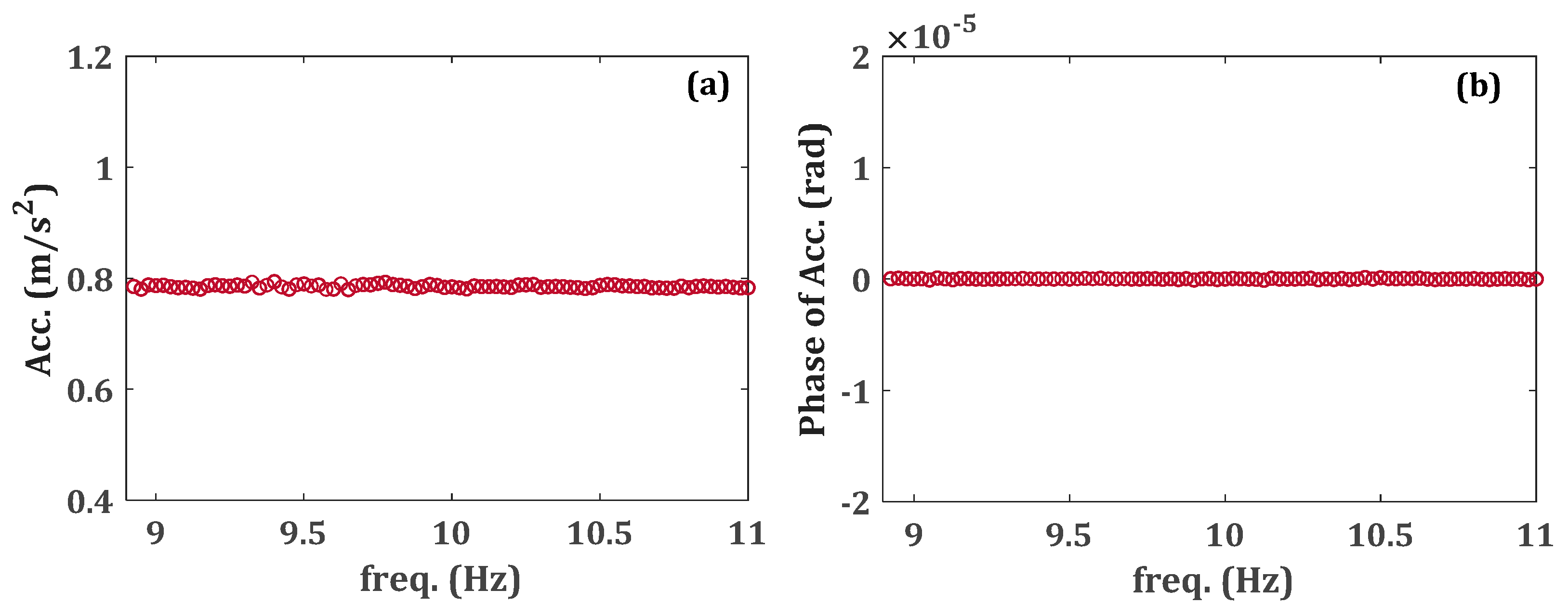
Figure 3 illustrates the constant acceleration base excitation for the frequency span of $f=\left[8.9–11\right]\mathrm{Hz}$. It is notable that the feedback of the response of the structure, particularly in the neighborhood of the resonant frequency, may change the amplitude of the excitation. Therefore, in order to keep the amplitude of the desired excitation constant, a sine test is carried out at each frequency point to measure the steady state response of the system. As a result, all of the experimental data measured from the sine test at each frequency step are utilized to find the frequency response of the system. To obtain all stable branches of the nonlinear response, both sweep-up and sweep-down tests were carried out. However, as the upper branch (with larger amplitude) is used in the optimization, only measuring the upper stable solution would be satisfactory. 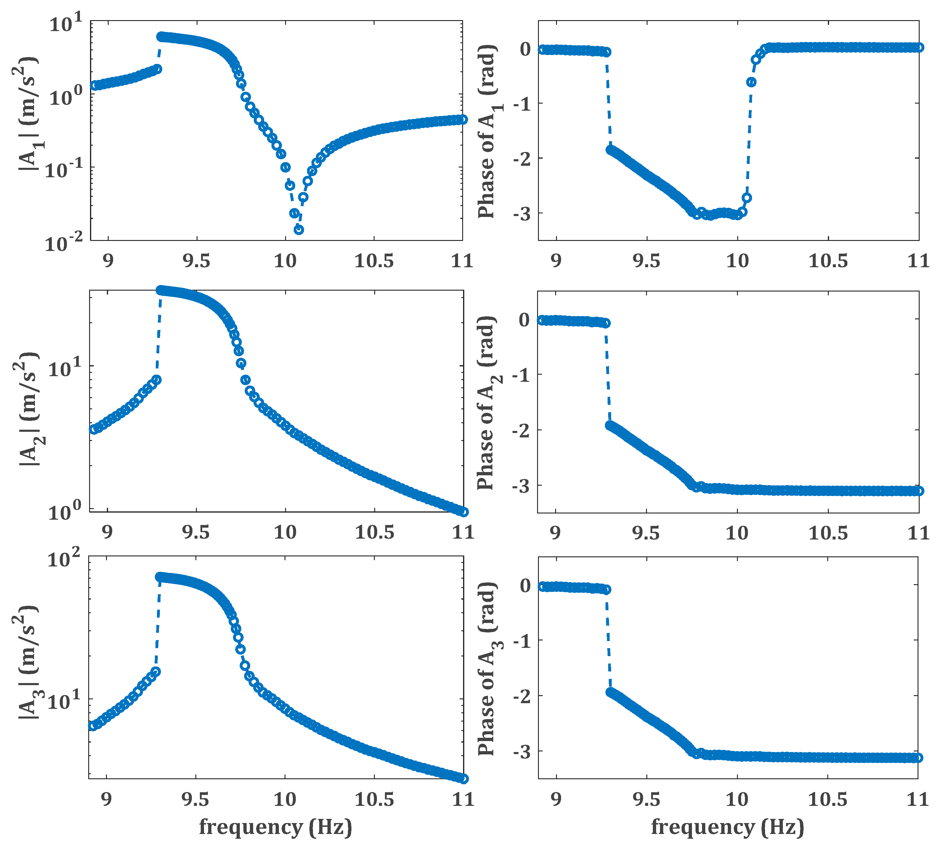For this study, as is explained in Section 3 and also shown in the measured nonlinear response, the electromagnets provide softening nonlinearities. Therefore, a sweep-down stepped-sine test is carried out to measure the upper branch of the response. The excitation amplitude should be large enough to guarantee that the nonlinearity of the system is excited. The amplitudes and phases of the experimentally measured nonlinear response of the system at three points along the beam, 5, 15, and 25 cm away from the clamped end of the beam (which are equivalent to the locations of AM1, AM2, and AM3), are shown in Figure 4. The measured nonlinear responses are used to identify the unknown nonlinear restoring force of the system.

In the following section, a mathematical model is derived for the nonlinear system corresponding to the experimental rig.

3. Mathematical Model

In this section, the nonlinear force obtained from the electromagnets explained in Section 2 is described by a mathematical model. A cantilever beam of length $L$, width $d$, thickness $h$, density $\rho$, and modulus of elasticity $E$ is considered. The cantilever is subjected to an unknown nonlinear electromagnetic restoring force $f_{NL}$ at the tip of the beam. The beam is mounted on a shaker base and is subject to base excitation.

The equation of motion of the system is derived using Lagrange’s equation. Since the type of nonlinearity is unknown, a mathematical form is assumed for the nonlinear force to be considered in the model. This assumption is based on the physics of the problem and also the measured nonlinear response of the system from experimental vibration tests. The attractive nonlinear force resulting from two symmetric electromagnets is generally given as [27,28],

$$f_{NL}=-\left(\frac{c_s}{{\left(d_0-\chi \right)}^2}-\frac{c_s}{{\left(d_0+\chi \right)}^2}\right),$$

(1)

where $\chi$ denotes the displacement of the tip of the beam, $d_0$ is the gap between each electromagnet and the tip at the equilibrium position, and $c_s$ is a positive constant coefficient dependant on the voltage of the electromagnets. Using the Taylor expansion about the equilibrium position ($\chi =0$), the nonlinear electromagnetic force of Equation (1) is rewritten as

$$f_{NL}=-\left(\frac{4c_s\chi }{d_0{}^3}+\frac{8c_s{\chi }^3}{d_0{}^5}+\frac{12c_s{\chi }^5}{d_0{}^7}+\frac{16c_s{\chi }^7}{d_0{}^9}+\cdots \right).$$

(2)

The negative sign of the force indicates that the attractive forces of two symmetric electromagnets generate softening nonlinearities in the system. Equation (2) may be used as an appropriate assumption for the nonlinear force with coefficients only dependent on the constants $c_s$ and $d_0$. However, it is often very difficult to have a purely symmetric electromagnetic force in an experiment. Moreover, the model of Equation (1) presented in [27] does not consider the damping effect of the electromagnetic force. Hence, in this study, a different framework will be considered to model the electromagnetic force. As shown in Equation (2), the Taylor series expansion may be used to represent the nonlinear stiffness force created by the electromagnets. Care has been taken to ensure that the configuration is symmetric and therefore we may assume only the odd terms are included. The damping force can be also represented by a Taylor series expansion. Based on this, four possible models to represent the nonlinearity of electromagnetic force are shown in

Table 2. Possible models to represent the electromagnetic force.

Model I:	$F_{nl}=\lambda \dot{\chi }+k_l\chi +k_{n_3}{\chi }^3,$	(3)
Model II	$F_{nl}=\lambda \dot{\chi }+k_l\chi +k_{n_3}{\chi }^3+k_{n_5}{\chi }^5$	(4)
Model III	$F_{nl}=\lambda \dot{\chi }+k_l\chi +k_{n_2}\chi \left|\chi \right|+k_{n_3}{\chi }^3+k_{n_5}{\chi }^5$	(5)
Model IV	$F_{nl}=\lambda \dot{\chi }+{\lambda }_n\dot{\chi }\left|\dot{\chi }\right|+k_l\chi +k_{n_2}\chi \left|\chi \right|+k_{n_3}{\chi }^3+k_{n_5}{\chi }^5$	(6)

. As can be seen in the table, the order of stiffness and damping nonlinearity is increased gradually. The level of nonlinearity is increased until it does not improve the identification results, and then the model may be considered good enough to represent the nonlinear electromagnetic force.

In Table 2 $\lambda ,{\lambda }_n$ denote the linear and nonlinear damping coefficients, and $k_l,k_{n_2},k_{n_3},k_{n_5}$ indicate the linear stiffness, symmetric quadratic stiffness, cubic and fifth order stiffnesses, respectively. Since the electromagnets are mounted on the movable bed of the shaker, as well as the beam, the displacement $\chi$ in Equations (3)–(6) should be the relative displacement of the tip of the beam.

Another important issue is to consider the effect of the aluminum L-shaped clamp to which the cantilever beam is attached. In fact, the beam under investigation is clamped between two short thick aluminum beams. These two aluminum support beams act like two very stiff springs attached to the base of the steel beam. Although the clamp is very stiff and will not undergo large deflections, it is not completely rigid. The high stiffness of the clamp may cause significant changes in the frequency response of the system, particularly in the frequencies of the resonances and anti-resonances of the system. Therefore, the effect of the very high stiffness of the clamp is simulated by a linear spring between the shaker bed and the base of cantilever. This linear spring represents the bending stiffness of the L-shaped clamp. It is worth noting that the deflection of the L-shaped clamp is in the same direction as the motion of the beam and the rotational motion of the clamped support acts in the torsional direction of the beam (as seen in Figure 5). Because the torsional motion of the beam is not considered in this study, there is no need for a rotational spring representing the torsional degree of freedom of the beam. All of the bolted joints are assumed to be rigidly connected in this model. The equivalent masses of two aluminum support beams are also taken into account as an additional mass. Figure 5 illustrates the equivalent system of the beam subject to the motion of shaker bed. The torsional deflection of the L-shaped clamp is assumed to be negligible, and hence the beam does not have any rotation at the base. Hence, the assumed mode shapes of the cantilever are used to simulate the dynamics of the beam. The equivalent mass $m_b$ and linear stiffness $k_b$ of the aluminum beams can be estimated by the following equations, [29].

$$m_b=\frac{33}{140}\left(2{\rho }_{Al}{V}_{Al}{}_b\right),\hspace{1em}{k}_b=\frac{3E_{Al}{I}_{Al}{}_b}{L_{Al}^3{}_b},$$

(7)

where ${\rho }_{Al}$ and $E_{Al}$ are density and modulus of elasticity of aluminium, respectively. $V_{Al}{}_b,I_{Al}{}_b$, and $L_{Al}{}_b$ denote, respectively, the volume, the second moment of area, and the length of each aluminium support beam.

Considering the assumed type of the nonlinearity and the effect of the clamp as a linear stiffness attached to the base of the beam, the governing equations of the system are derived using the Euler-Lagrange method. In this case, the equation of motion will be derived for case IV but the obtained solution for the nonlinear frequency response functions may be used for the three simpler models, i.e. Model I ($k_{n_5}=k_{n_2}={\lambda }_n=0$), Model II ($k_{n_2}={\lambda }_n=0$) and Model III (${\lambda }_n=0$). The kinetic and potential energy are given as follows

$$T=\frac{1}{2}{{\displaystyle \int }}_0^l\rho A{\left(\frac{\partial w\left(x,t\right)}{\partial t}\right)}^{2}dx+\frac{1}{2}{\displaystyle \sum }_{n=1}^{N_p}{M}_n{\left(\frac{\partial w\left(x,t\right)}{\partial t}\right)}^2\delta \left(x-x_n\right),$$

(8)

$$\begin{array}{cc}\hfill V& =\frac{1}{2}{{\displaystyle \int }}_0^{l}EI{\left(\frac{{\partial }^2\left(w\left(x,t\right)-w_b\left(t\right)\right)}{\partial x^2}\right)}^2+\frac{1}{2}{k}_b{\left(w\left(0,t\right)-w_b\left(t\right)\right)}^2\hfill \\ & +\frac{1}{2}{k}_l{\left(w\left(l,t\right)-w_b\left(t\right)\right)}^2+\frac{1}{3}{k}_{n_2}{\left(w\left(l,t\right)-w_b\left(t\right)\right)}^2\left|w\left(l,t\right)-w_b\left(t\right)\right|\hfill \\ & +\frac{1}{4}{k}_{n_3}{\left(w\left(l,t\right)-w_b\left(t\right)\right)}^4+\frac{1}{6}{k}_{n_5}{\left(w\left(l,t\right)-w_b\left(t\right)\right)}^6,\hfill \end{array}$$

(9)

where $w\left(x,t\right)$ is the transverse vibration of the beam, $x$ is the distance from the clamped end of the beam, $w_b\left(t\right)$ is the base motion of the shaker in the transverse direction of the beam, $M_n$ denotes all additional masses including accelerometers, permanent magnets attached to the tip, and the equivalent mass of the clamp support, and $N_p$ is the total number of additional masses. Defining $z\left(x,t\right)$ as the relative displacement of the beam with respect to the base motion $w_b\left(t\right)$ of the shaker bed, then

$$z\left(x,t\right)=w\left(x,t\right)-w_b\left(t\right),$$

(10)

and the kinetic and potential energy can be rewritten as,

$$T=\frac{1}{2}{{\displaystyle \int }}_0^l\rho A{\left(\frac{\partial \left(z\left(x,t\right)+w_b\left(t\right)\right)}{\partial t}\right)}^{2}dx+\frac{1}{2}{\displaystyle \sum }_{n=1}^{N_p}{M}_n{\left(\frac{\partial \left(z\left(x,t\right)+w_b\left(t\right)\right)}{\partial t}\right)}^2\delta \left(x-x_n\right),$$

(11)

$$\begin{gathered} V=\frac{1}{2}{{\displaystyle \int }}_0^{l}EI{\left(\frac{{\partial }^{2}z\left(x,t\right)}{\partial x^2}\right)}^2+\frac{1}{2}{k}_b{\left(z\left(0,t\right)\right)}^2+\frac{1}{2}{k}_l{\left(z\left(l,t\right)\right)}^2+\frac{1}{3}{k}_{n_2}{\left(z\left(l,t\right)\right)}^2\left|z\left(l,t\right)\right| \\ +\frac{1}{4}{k}_{n_3}{\left(z\left(l,t\right)\right)}^4+\frac{1}{6}{k}_{n_5}{\left(z\left(l,t\right)\right)}^6, \end{gathered}$$

(12)

Considering the proportional damping for the beam, Rayleigh’s dissipation function of the system is also derived as,

$$\begin{gathered} D=\frac{1}{2}{{\displaystyle \int }}_0^l\left\{\alpha {\left(\frac{\partial z\left(x,t\right)}{\partial t}\right)}^2+\beta {\left(\frac{{\partial }^{3}z\left(x,t\right)}{\partial x^2\partial t}\right)}^2\right\}dx+\frac{1}{2}\lambda {\left(\frac{\partial z\left(l,t\right)}{\partial t}\right)}^2 \\ +\frac{1}{3}{\lambda }_n{\left(\frac{\partial z\left(l,t\right)}{\partial t}\right)}^2\left|\frac{\partial z\left(l,t\right)}{\partial t}\right|, \end{gathered}$$

(13)

where $\alpha ,\beta$ are the proportional damping coefficients per length of the beam. Using the Euler-Lagrange equation, along with the assumed mode method, the equation of motion of the system is derived. For this purpose, a solution is assumed for the response of the beam as

$$z\left(x,t\right)={\displaystyle \sum }_{i=1}^{N_m}{\varphi }_i\left(x\right)q_i\left(t\right),$$

(14)

where $N_m$ represents the total number of modes used in the analysis, $q_i$ denotes the $i-$th time variable modal coordinate, and ${\varphi }_i$ is the $i-$th mode shape of the beam with the following boundary conditions

$$\begin{gathered} \frac{\partial z}{\partial x}=0,\hspace{1em}\frac{\partial }{\partial x}\left(EI\frac{{\partial }^{2}z}{\partial x^2}\right)=-k_{b}z\left(x,t\right),\hspace{1em}x=0, \\ EI\frac{{\partial }^{2}z}{\partial x^2}=0,\hspace{1em}\frac{\partial }{\partial x}\left(EI\frac{{\partial }^{2}z}{\partial x^2}\right)=0,\hspace{1em}x=l, \end{gathered}$$

(15)

In this study, a single-mode approximation of the system is utilized for the identification process. Therefore, the equations of motion are derived for this single-mode approximation. For the sake of brevity, the subscripts related to the first mode are neglected. In order to apply the assumed mode method, the quadratic stiffness and damping energy terms of Equations (12) and (13) that include absolute functions can be approximated using following series,

$$\begin{array}{cc}\hfill \frac{1}{3}{k}_{n_2}{z}^2\left|z\right|& \hfill =\frac{1}{3}{k}_{n_2}z\left(\left(\frac{2}{\pi }\right)z-\left(\frac{4}{\pi }\right)z{\displaystyle {\displaystyle \sum }_{i=1}^{\infty }}\left(\frac{{\left(-1\right)}^i{T}_{2i}\left(z\right)}{-1+4i^2}\right)\right)\\ & \hfill =k_{n_2}\left(\frac{1}{2}{c}_1{z}^2+\frac{1}{4}{c}_3{z}^4+\frac{1}{6}{c}_5{z}^6+\cdots \right),\\ \hfill \frac{1}{3}{\lambda }_n{\dot{z}}^2\left|\dot{z}\right|& \hfill =\frac{1}{3}{\lambda }_n\dot{z}\left(\left(\frac{2}{\pi }\right)\dot{z}-\left(\frac{4}{\pi }\right)\dot{z}{\displaystyle {\displaystyle \sum }_{i=1}^{\infty }}\left(\frac{{\left(-1\right)}^i{T}_{2i}\left(\dot{z}\right)}{-1+4i^2}\right)\right)\\ & \hfill ={\lambda }_n\left(\frac{1}{2}{e}_1{\dot{z}}^2+\frac{1}{4}{e}_3{\dot{z}}^4+\frac{1}{6}{e}_5{\dot{z}}^6+\cdots \right),\end{array}$$

(16)

where $c_1,c_3,c_5,\dots$ and $e_1,e_3,e_5,\dots$ are the coefficients of the approximations of Equations (16), and $T_n\left(z\right)$ is the Chebyshev polynomial of the first kind, for example

$$T_{10}\left(z\right)=-1+50z^2-400z^4+1120z^6-1280z^8+512z^{10},$$

(17)

Given the approximations of Equation (16) for the quadratic stiffness and damping terms, substituting the assumed solution of Equation (14) into Equations (11)–(13), and applying the Euler-Lagrange method, the equation of motion is obtained as

$$\begin{gathered} \left(\rho A{R}_1+{\displaystyle \sum }_{n=1}^{N_p}{M}_n{R}_{2_n}\right)\ddot{q}+\left(\alpha R_1+\beta R_3\right)\dot{q}+EI{R}_{3}q+\lambda R_4\dot{q}+{\lambda }_n{g}_{nl}\left(\dot{q}\right)+k_b{R}_{4}q \\ +k_l{R}_{5}q+k_{n_2}{h}_{nl}\left(q\right)+k_{n_3}{R}_7{q}^3+k_{n_5}{R}_8{q}^5 \\ =-\left(\rho A{R}_0+{\displaystyle \sum }_{n=1}^{N_p}{M}_n{R}_{0_n}\right){\ddot{w}}_b, \end{gathered}$$

(18)

where $q$ denotes the time variable modal coordinate of first mode,

$$\begin{array}{cccc}{R}_0={{\displaystyle \int }}_0^l{\varphi }_{1}dx,& R_{0_n}=\left({\varphi }_1\right){|}_{x_n},& R_1={{\displaystyle \int }}_0^l{\varphi }_1^{2}dx,& R_{2_n}=\left({\varphi }_1^2\right){|}_{x_n},\\ & R_3={{\displaystyle \int }}_0^l{\varphi }_1^{″}{}^{2}dx,& R_4=\left({\varphi }_1^2\right){|}_{x=0},& R_5=\left({\varphi }_1^2\right){|}_{x=l},\\ & R_7=\left({\varphi }_1^4\right){|}_{x=l},& R_8=\left({\varphi }_1^6\right){|}_{x=l}& \end{array}$$

(19)

and

$$\begin{gathered} g_{nl}\left(\dot{q}\right)=\left(e_1{R}_4\right)\dot{q}+\left(e_3{R}_7\right){\dot{q}}^3+\left(e_5{R}_8\right){\dot{q}}^5+\cdots \\ {h}_{nl}\left(q\right)=\left(c_1{R}_4\right)q+\left(c_3{R}_7\right)q^3+\left(c_5{R}_8\right)q^5+\cdots \end{gathered}$$

(20)

There are many methods that are able to solve the nonlinear differential equations of motion [28,30]. In this study, the Harmonic Balance Method (HBM) is used to investigate the steady state dynamics of the system.

As the primary harmonic is dominant in the nonlinear response of the system, the higher harmonics are neglected in this paper. Hence, in order to apply the HBM to the equations of motion (Equation (18)) of the system, the periodic time variable response $q\left(t\right)$ of the system is assumed to be

$$q\left(t\right)=a\left(t\right)\sin \left(\mathsf{\Omega }t\right)+b\left(t\right)\cos \left(\mathsf{\Omega }t\right),$$

(21)

The slowly varying sine and cosine coefficients $a\left(t\right)$ and $b\left(t\right)$ are considered time-variant to study the transient response of the system. However, in this paper only the steady-state behavior is examined. Since the coefficients $a\left(t\right)$ and $b\left(t\right)$ are slow-varying, $\ddot{a}$ and $\ddot{b}$ are neglected in the analysis. Accordingly, the time derivatives of the time variable $q\left(t\right)$ of the response are obtained as

$$\begin{gathered} \dot{q}\left(t\right)=\left(\dot{b}+\mathsf{\Omega }a\right)\cos \left(\mathsf{\Omega }t\right)+\left(\dot{a}-b\mathsf{\Omega }\right)\sin \left(\mathsf{\Omega }t\right), \\ \ddot{q}\left(t\right)=\mathsf{\Omega }\left(2\dot{a}-b\mathsf{\Omega }\right)\cos \left(\mathsf{\Omega }t\right)-\mathsf{\Omega }\left(2\dot{b}+a\mathsf{\Omega }\right)\sin \left(\mathsf{\Omega }t\right) \end{gathered}$$

(22)

Substituting Equations (21) and (22) into Equation (18) and balancing the coefficients of $\sin \left(\mathsf{\Omega }t\right)$ and $\cos \left(\mathsf{\Omega }t\right)$, two differential equations are obtained as follows.

$$\begin{gathered} 2P_1\mathsf{\Omega }\dot{a}+P_2\dot{b}=P_{1}b{\mathsf{\Omega }}^2-P_{2}a\mathsf{\Omega }-P_{3}b-P_4{C}_{g_{nl}}-P_5{C}_{h_{nl}}-P_6{C}_{q3}-P_7{C}_{q5}, \\ {P}_2\dot{a}-2P_1\mathsf{\Omega }\dot{b}=P_8+P_{1}a{\mathsf{\Omega }}^2+P_{2}b\mathsf{\Omega }-P_{3}a-P_4{S}_{g_{nl}}-P_5{S}_{h_{nl}}-P_6{S}_{q3}-P_7{S}_{q5}, \end{gathered}$$

(23)

where

$$\begin{gathered} P_1=\rho A{R}_1+{\displaystyle \sum }_{n=1}^{N_p}{M}_n{R}_{2_n},\hspace{1em}{P}_2=\alpha R_1+\beta R_3+\lambda R_4,\hspace{1em}{P}_3=k_b{R}_4+EI{R}_3+k_l{R}_4, \\ {P}_4={\lambda }_n,\hspace{1em}{P}_5=k_{n_2},\hspace{1em}{P}_6=k_{n_3}{R}_7,\hspace{1em}{P}_7=k_{n_5}{R}_8, \\ {P}_8=-\left(\rho A{R}_0+{\displaystyle \sum }_{n=1}^{N_p}{M}_n{R}_{0_n}\right)W_b, \\ {C}_{g_{nl}}=\left(e_1{R}_4\right)\left(\dot{b}+\mathsf{\Omega }a\right)+\left(e_3{R}_7\right)C_{qd3}+\left(e_5{R}_8\right)C_{qd5}+\cdots \\ {C}_{g_{nl}}=\left(e_1{R}_4\right)\left(\dot{b}+\mathsf{\Omega }a\right)+\left(e_3{R}_7\right)C_{qd3}+\left(e_5{R}_8\right)C_{qd5}+\cdots \\ {S}_{g_{nl}}=\left(e_1{R}_4\right)\left(\dot{a}-b\mathsf{\Omega }\right)+\left(e_3{R}_7\right)S_{qd3}+\left(e_5{R}_8\right)S_{qd5}+\cdots \\ {C}_{h_{nl}}=\left(c_1{R}_4\right)b+\left(c_3{R}_7\right)C_{q3}+\left(c_5{R}_8\right)C_{q5}+\cdots \\ {S}_{h_{nl}}=\left(c_1{R}_4\right)a+\left(c_3{R}_7\right)C_{q3}+\left(c_5{R}_8\right)C_{q5}+\cdots \end{gathered}$$

(24)

and

$$\begin{gathered} S_{q3}=\frac{3}{4}{a}^3+\frac{3}{2}a{b}^2, \\ {C}_{q3}=\frac{3}{2}{a}^{2}b+\frac{3}{4}{b}^3, \\ {S}_{q5}=\frac{5}{8}{a}^5+\frac{15}{4}{a}^3{b}^2+\frac{15}{8}a{b}^4 \\ {C}_{q5}=\frac{15}{8}{a}^{4}b+\frac{15}{4}{a}^2{b}^3+\frac{5}{8}{b}^5 \\ \begin{array}{cc}\hfill S_{qd3}=\frac{3}{2}{a}^2\dot{a}{\mathsf{\Omega }}^2& -\frac{3}{2}{a}^{2}b{\mathsf{\Omega }}^3+3a\dot{a}\dot{b}\mathsf{\Omega }-3ab\dot{b}{\mathsf{\Omega }}^2+\frac{3}{4}{\dot{a}}^3-\frac{9}{4}{\dot{a}}^{2}b\mathsf{\Omega }+\frac{9}{4}\dot{a}{b}^2{\mathsf{\Omega }}^2+\frac{3}{2}\dot{a}{\dot{b}}^2-\frac{3}{4}{b}^3{\mathsf{\Omega }}^3\hfill \\ & -\frac{3}{2}b{\dot{b}}^2\mathsf{\Omega }\hfill \\ \hfill C_{qd3}=\frac{3}{4}{a}^3{\mathsf{\Omega }}^3& +\frac{9}{4}{a}^2\dot{b}{\mathsf{\Omega }}^2+\frac{3}{2}a{\dot{a}}^2\mathsf{\Omega }-3a\dot{a}b{\mathsf{\Omega }}^2+\frac{3}{2}a{b}^2{\mathsf{\Omega }}^3+\frac{9}{4}a{\dot{b}}^2\mathsf{\Omega }+\frac{3}{2}{\dot{a}}^2\dot{b}-3\dot{a}b\dot{b}\mathsf{\Omega }\hfill \\ & +\frac{3}{2}{b}^2\dot{b}{\mathsf{\Omega }}^2+\frac{3}{4}{\dot{b}}^3\hfill \\ \hfill S_{qd5}=\frac{15}{8}{a}^4\dot{a}{\mathsf{\Omega }}^4& -\frac{15}{8}{a}^{4}b{\mathsf{\Omega }}^5+\frac{15}{2}{a}^3\dot{a}\dot{b}{\mathsf{\Omega }}^3-\frac{15}{2}{a}^{3}b\dot{b}{\mathsf{\Omega }}^4+\frac{15}{4}{a}^2{\dot{a}}^3{\mathsf{\Omega }}^2-\frac{45}{4}{a}^2{\dot{a}}^{2}b{\mathsf{\Omega }}^3\hfill \\ & +\frac{45}{4}{a}^2\dot{a}{b}^2{\mathsf{\Omega }}^4+\frac{45}{4}{a}^2\dot{a}{\dot{b}}^2{\mathsf{\Omega }}^2-\frac{15}{4}{a}^2{b}^3{\mathsf{\Omega }}^5-\frac{45}{4}{a}^{2}b{\dot{b}}^2{\mathsf{\Omega }}^3+\frac{15}{2}a{\dot{a}}^3\dot{b}\mathsf{\Omega }\hfill \\ & -\frac{45}{2}a{\dot{a}}^{2}b\dot{b}{\mathsf{\Omega }}^2+\frac{45}{2}a\dot{a}{b}^2\dot{b}{\mathsf{\Omega }}^3+\frac{15}{2}a\dot{a}{\dot{b}}^3\mathsf{\Omega }-\frac{15}{2}a{b}^3\dot{b}{\mathsf{\Omega }}^4-\frac{15}{2}ab{\dot{b}}^3{\mathsf{\Omega }}^2+\frac{5}{8}{\dot{a}}^5\hfill \\ & -\frac{25}{8}{\dot{a}}^{4}b\mathsf{\Omega }+\frac{25}{4}{\dot{a}}^3{b}^2{\mathsf{\Omega }}^2+\frac{15}{4}{\dot{a}}^3{\dot{b}}^2-\frac{25}{4}{\dot{a}}^2{b}^3{\mathsf{\Omega }}^3-\frac{45}{4}{\dot{a}}^{2}b{\dot{b}}^2\mathsf{\Omega }+\frac{25}{8}\dot{a}{b}^4{\mathsf{\Omega }}^4\hfill \\ & +\frac{45}{4}\dot{a}{b}^2{\dot{b}}^2{\mathsf{\Omega }}^2+\frac{15}{8}\dot{a}{\dot{b}}^4-\frac{5}{8}{b}^5{\mathsf{\Omega }}^5-\frac{15}{4}{b}^3{\dot{b}}^2{\mathsf{\Omega }}^3-\frac{15}{8}b{\dot{b}}^4\mathsf{\Omega }\hfill \\ \hfill C_{qd5}=\frac{5}{8}{a}^5{\mathsf{\Omega }}^5& +\frac{25}{8}{a}^4\dot{b}{\mathsf{\Omega }}^4+\frac{15}{4}{a}^3{\dot{a}}^2{\mathsf{\Omega }}^3-\frac{15}{2}{a}^3\dot{a}b{\mathsf{\Omega }}^4+\frac{15}{4}{a}^3{b}^2{\mathsf{\Omega }}^5+\frac{25}{4}{a}^3{\dot{b}}^2{\mathsf{\Omega }}^3\hfill \\ & +\frac{45}{4}{a}^2{\dot{a}}^2\dot{b}{\mathsf{\Omega }}^2-\frac{45}{2}{a}^2\dot{a}b\dot{b}{\mathsf{\Omega }}^3+\frac{45}{4}{a}^2{b}^2\dot{b}{\mathsf{\Omega }}^4+\frac{25}{4}{a}^2{\dot{b}}^3{\mathsf{\Omega }}^2+\frac{15}{8}a{\dot{a}}^4\mathsf{\Omega }\hfill \\ & -\frac{15}{2}a{\dot{a}}^{3}b{\mathsf{\Omega }}^2+\frac{45}{4}a{\dot{a}}^2{b}^2{\mathsf{\Omega }}^3+\frac{45}{4}a{\dot{a}}^2{\dot{b}}^2\mathsf{\Omega }-\frac{15}{2}a\dot{a}{b}^3{\mathsf{\Omega }}^4\hfill \\ & -\frac{45}{2}a\dot{a}b{\dot{b}}^2{\mathsf{\Omega }}^2+\frac{15}{8}a{b}^4{\mathsf{\Omega }}^5+\frac{45}{4}a{b}^2{\dot{b}}^2{\mathsf{\Omega }}^3+\frac{25}{8}a{\dot{b}}^4\mathsf{\Omega }+\frac{15}{8}{\dot{a}}^4\dot{b}\hfill \\ & -\frac{15}{2}{\dot{a}}^{3}b\dot{b}\mathsf{\Omega }+\frac{45}{4}{\dot{a}}^2{b}^2\dot{b}{\mathsf{\Omega }}^2+\frac{15}{4}{\dot{a}}^2{\dot{b}}^3-\frac{15}{2}\dot{a}{b}^3\dot{b}{\mathsf{\Omega }}^3-\frac{15}{2}\dot{a}b{\dot{b}}^3\mathsf{\Omega }\hfill \\ & +\frac{15}{8}{b}^4\dot{b}{\mathsf{\Omega }}^4+\frac{15}{4}{b}^2{\dot{b}}^3{\mathsf{\Omega }}^2+\frac{5}{8}{\dot{b}}^5\hfill \end{array} \end{gathered}$$

(25)

where $W_b$ is the amplitude of the base acceleration ${\ddot{w}}_b$. In order to find the steady-state response of the system, the time-variant terms in Equation (23) are set to zero. Consequently, the nonlinear differential equation of motion is transformed into two nonlinear algebraic equations as follows

$$\begin{gathered} P_{1}b{\mathsf{\Omega }}^2-P_{2}a\mathsf{\Omega }-P_{3}b-P_4{C}_{g_{SS}}-P_5{C}_{h_{SS}}-P_6{C}_{q3}-P_7{C}_{q5}=0, \\ {P}_8+P_{1}a{\mathsf{\Omega }}^2+P_{2}b\mathsf{\Omega }-P_{3}a-P_4{S}_{g_{SS}}-P_5{S}_{h_{SS}}-P_6{S}_{q3}-P_7{S}_{q5}=0, \end{gathered}$$

(26)

where

$$\begin{gathered} \begin{array}{cc}\hfill C_{g_{SS}}=\left(e_1{R}_4\right)& \left(\mathsf{\Omega }a\right)+\left(e_3{R}_7\right)\left(\frac{3}{4}{a}^3{\mathsf{\Omega }}^3+\frac{3}{2}a{b}^2{\mathsf{\Omega }}^3\right)\hfill \\ & +\left(e_5{R}_8\right)\left(\frac{5}{8}{a}^5{\mathsf{\Omega }}^5+\frac{15}{4}{a}^3{b}^2{\mathsf{\Omega }}^5+\frac{15}{8}a{b}^4{\mathsf{\Omega }}^5\right)+\cdots \hfill \\ \hfill S_{g_{SS}}=\left(e_1{R}_4\right)\left(b\mathsf{\Omega }\right)& +\left(e_3{R}_7\right)\left(-\frac{3}{2}{a}^{2}b{\mathsf{\Omega }}^3-\frac{3}{4}{b}^3{\mathsf{\Omega }}^3\right)\hfill \\ & +\left(e_5{R}_8\right)\left(-\frac{15}{8}{a}^{4}b{\mathsf{\Omega }}^5-\frac{15}{4}{a}^2{b}^3{\mathsf{\Omega }}^5-\frac{5}{8}{b}^5{\mathsf{\Omega }}^5\right)+\cdots \hfill \end{array} \\ {C}_{h_{SS}}=\left(c_1{R}_4\right)b+\left(c_3{R}_7\right)\left(\frac{3}{2}{a}^{2}b+\frac{3}{4}{b}^3\right)+\left(c_5{R}_8\right)\left(\frac{15}{8}{a}^{4}b+\frac{15}{4}{a}^2{b}^3+\frac{5}{8}{b}^5\right)+\cdots \\ {S}_{h_{SS}}=\left(c_1{R}_4\right)a+\left(c_3{R}_7\right)\left(\frac{3}{4}{a}^3+\frac{3}{2}a{b}^2\right)+\left(c_5{R}_8\right)\left(\frac{5}{8}{a}^5+\frac{15}{4}{a}^3{b}^2+\frac{15}{8}a{b}^4\right)+\cdots \end{gathered}$$

(27)

Different numerical methods may be used to solve the nonlinear algebraic equations. Here, in this study, the resultant nonlinear algebraic equations of Equation (26) are solved using the arc-length continuation method. The amplitude-frequency response of the system obtained from the numerical method is used in the optimization process to identify the nonlinear system. The following section explains the optimization process.

4. Nonlinear Identification

There are different methods introduced to identify the nonlinearities in the system. One of the biggest weaknesses of most of these methods is the accumulative error in the results of the identification process. Errors from various sources are accumulated in the identification process leading to a considerable error in the identified values of the parameters. Using the measured frequency domain data directly in the identification of parameters reduces such errors to the lowest possible. One significant error is when the low amplitude response of a nonlinear mechanical structure is used to update the underlying linear system. Although the effect of nonlinearity on the response of the system is at its lowest level for very low amplitude excitation, this effect cannot be eliminated from the measured response it can affect the results of the updating procedure. Therefore, some modelling error appears in the underlying linear system.

In many practical engineering structures, it is not possible to have spatially complete measurements. However, some of the finite element-based identification methods require all coordinates to be measured [21,22]. Hence, various expansion methods, such as the System Equivalent Reduction Expansion Process (SEREP), may be used to estimate the unmeasured coordinates, which may cause error in the final results of the identification process. Avoiding expansion methods would eliminate the possible error in this process. The approach presented in this study aims to eliminate the aforementioned errors in the process of nonlinear identification.

The proposed method is composed of two main steps. In the first step, a linear model updating method is applied to the linear response of a low amplitude test. The resultant updated parameters are used as an appropriate initial guess for the underlying linear system. The updated parameters of the underlying linear system are then corrected in step two. By correcting the updated parameters obtained from the first step, the above-discussed error due to the effect of nonlinearity in the low amplitude response of the system is avoided.

The second step is to identify the underlying linear system and the nonlinear restoring force utilizing the updated linear model and nonlinear experimental response in an optimization process. To this end, a nonlinear form is assumed for the nonlinearity corresponding to the experimental response. Here, good engineering insight is required to have an appropriate assumed model. Consequently, a numerical model is developed for the nonlinear system using the assumed nonlinear force with estimated linear parameters to be corrected and unknown nonlinear parameters to be estimated. Then, the optimized values of the system parameters are targeted considering an objective function defined by minimizing the difference between the experimental and analytical responses at the measured coordinates, [31], as

$$J=\min \left({\displaystyle \sum }_{i=1}^{N_f}\left|\log \left(X_m{\left({\Omega }_i\right)}_2\right)-\log \left(X_a{\left({\Omega }_i\right)}_2\right)\right|\right),$$

(28)

where $X_m$ and $X_a$ denote respectively the experimental and numerical responses of the system in the frequency domain at the measured points. Using the logarithmic scale in the objective function penalizes large changes between optimized and experimental responses. Considering only measured coordinates in the identification procedure eliminates the need for a spatially complete measurement and the need to use expansion methods. Therefore, the associated error is eliminated from the calculations. $N_f$ is the number of measured frequency lines considered in the optimization. The optimized parameters are subjected to different constraints limiting the solution range of the objective function. For instance, the optimized parameters must have values within the allowable range. Some data selection criteria may be applied to the frequency response before being used in the optimization process as follows:

(a) The first data selection is to narrow the frequency response to a range in which the effect of the nonlinearity is considerable. By applying this criterion, the calculation cost is reduced significantly, because there is no significant difference between the linear and the nonlinear responses in the regions which are insensitive to the nonlinearity.

(b) The second is to neglect the unstable branches of the numerical solution which are not measured in the experimental tests.

(c) The third data selection criterion is to choose between the solutions in the multi-response regions. Having more than one solution at a single frequency line may cause the optimization process to slow down or, in some cases, not to converge to a reasonable solution. In this case, usually the upper solution branch (having the larger amplitude) is selected, because the effect of the nonlinearity is more significant compared to the lower branch. Of course, the selected branch must correspond to the experimentally measured response used in the optimization. The lower branch of the response or the responses of different excitation levels can be used to make sure that the results of the optimization are correct.

Applying all the constraints and criteria described above, the parameters of the assumed model of the nonlinear system are optimized. These values are used to estimate the linear (low amplitude test) and nonlinear response (high amplitude test) of the system. If an acceptable match is not observed between the experimentally measured response and the estimated response, the assumed form of the nonlinear force is revised, and the optimization process is repeated. This process is carried out until a good correlation between the experimental results and the analytical model is achieved.

5. Results and Discussion

In this section, first the results of the linear model updating are presented and compared with the experimental linear response of the system. Afterwards, the results of the identification of the unknown nonlinear force of the system are discussed.

In order to identify the structural model of the cantilever beam, first the underlying linear model is updated using linear updating methods [2,3,4]. For this purpose, the linear response of the nonlinear system is measured by exciting the structure with very low amplitude base excitation. The first three measured natural frequencies are used to update the underlying linear system. Three parameters of the system are updated, namely the flexural stiffness $EI$, the base stiffness $k_b$, and the base mass $m_b$. After updating these three parameters using the natural frequencies, the proportional damping coefficients $\alpha ,\beta$ are updated.

Table 3. Parameters used in the linear model updating.

	Parameters		Parameter Values (in SI Units)
	Description of Parameters		Initial Values	Updated Values
Fixed Parameters	Mass of the accelerometers (kg)	$m_a$	$0.008$	-
	Mass of the permanent magnets (kg)	$m_p$	$0.004$	-
	Linear mass per unit length of the beam (kg/m)	$\rho A$	$0.368$	-
	Length of the beam (m)	$L$	$0.3$	-
Updated parameters	Proportional damping coefficient	$\alpha$	0.2	0.294
	Proportional damping coefficient	$\beta$	$1\times {10}^{-5}$	$1.33\times {10}^{-5}$
	Flexural stiffness of the beam (Nm2)	$EI$	$1.741$	1.64
	Equivalent stiffness of the clamp support (N/m)	$k_b$	$8.256\times {10}^5$	$5.5\times {10}^5$
	Equivalent mass of the clamp support (kg)	$m_b$	$0.1016$	$0.103$

gives the values of the fixed and updated parameters of the system.

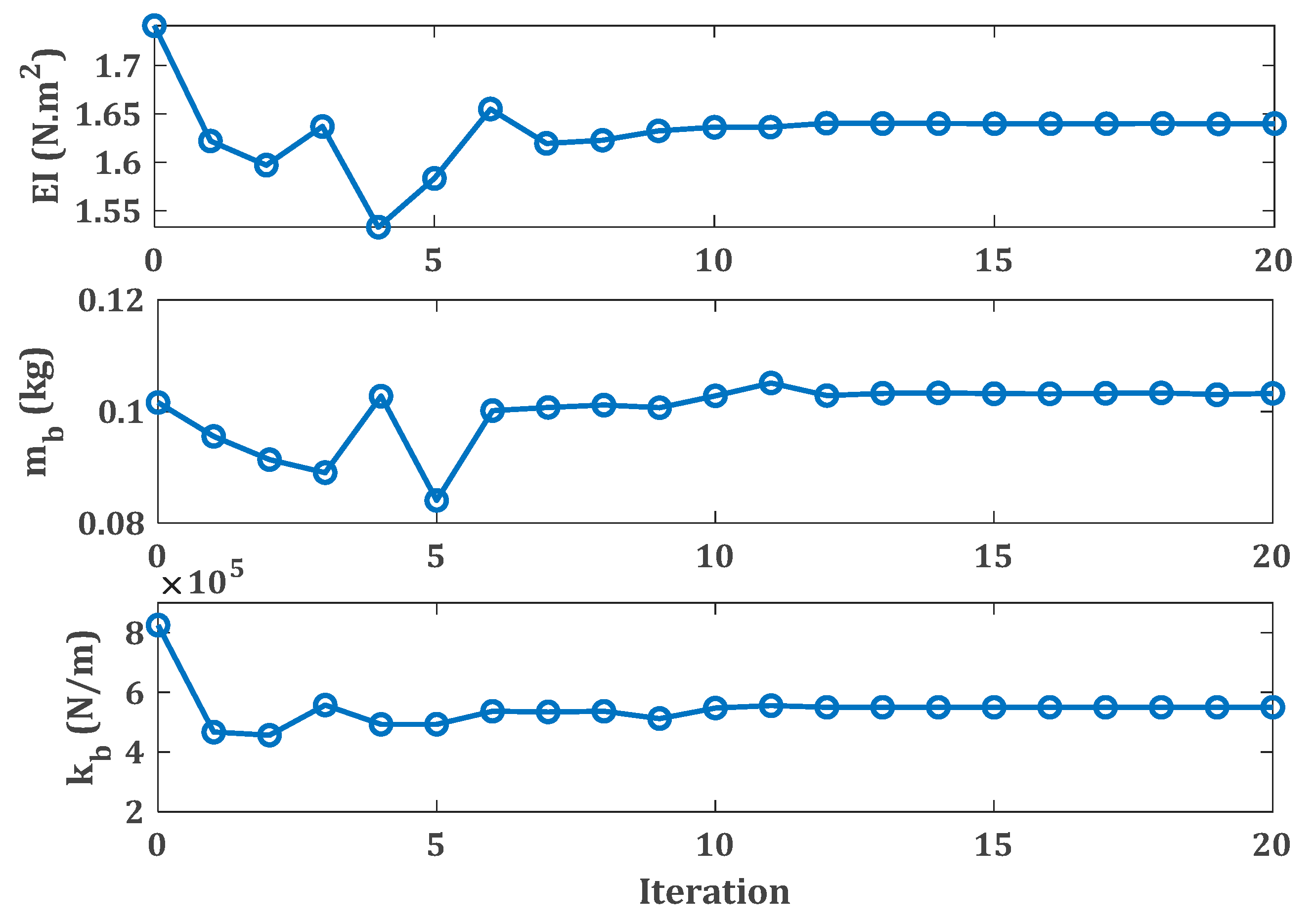
$EI$, $k_b$ and $m_b$ are updated using measured natural frequencies as shown in Figure 6. Figure 7 illustrates that after 20 iterations, the updated natural frequencies predicated by the numerical model are in excellent agreement with those obtained experimentally.

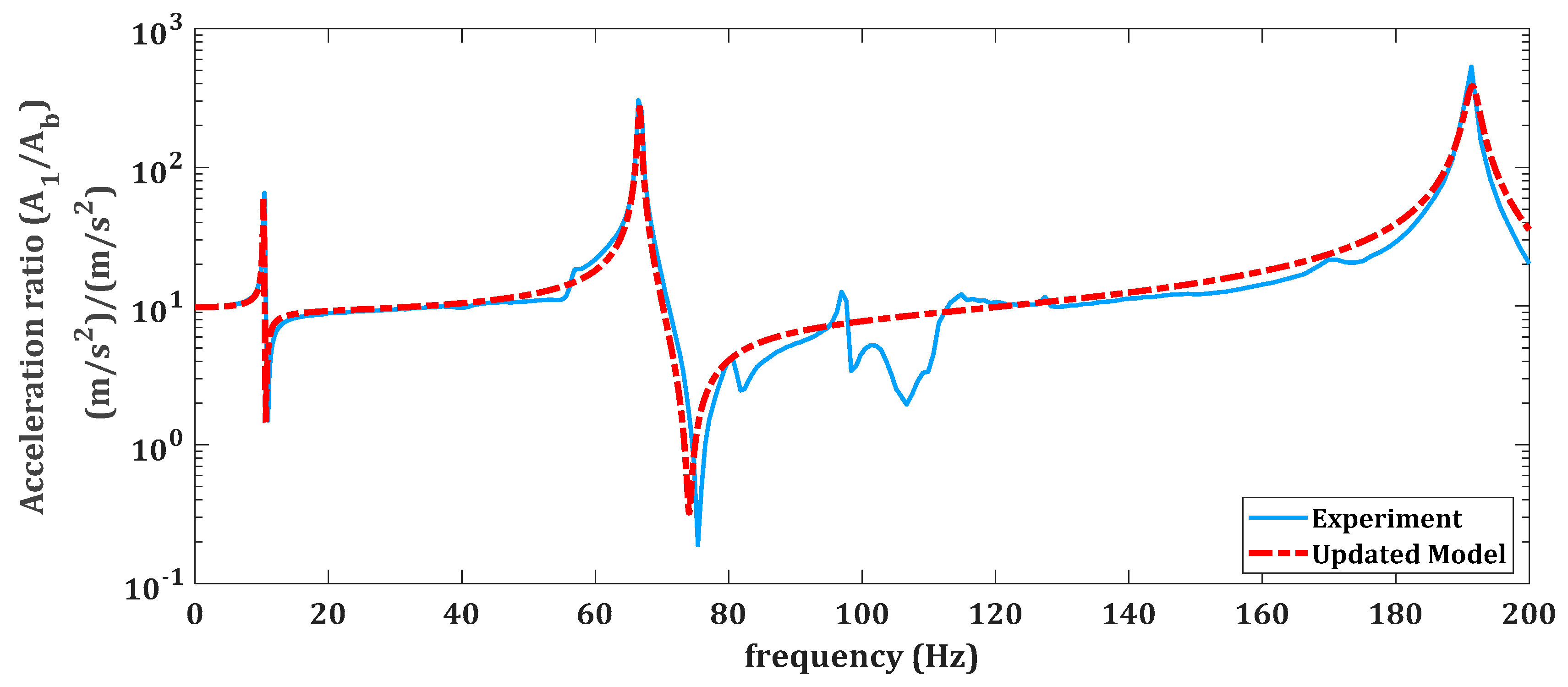
Having updated the parameters, the numerical linear frequency response is obtained using the updated linear model of the underlying linear structure. Figure 8 shows the experimental and updated linear frequency response of the system at the location of 1st accelerometer (AM1) for the frequency range containing the first three modes. A very important observation is that the updated model can estimate the anti-resonance frequencies, which are not included in the updating method. Therefore, the good agreement between both the resonance and anti-resonance frequencies shows the updated linear model is valid. The low-amplitude experimental and updated analytical linear responses are compared in Figure 9 in the neighborhood of the first natural frequency in the presence of the nonlinear electromagnetic force.

Given the updated model of the underlying linear system, the nonlinear system is now identified. For this purpose, the nonlinear amplitude-frequency response of the system at the location of 3rd accelerometer (AM3) is used in optimization process to identify the nonlinear force. As expected from Equation (2), the response of the system demonstrates a softening nonlinearity in the system. Having the updated underlying linear system, the measured nonlinear response of the system is utilized in the optimization process to estimate the unknown parameters of the nonlinear force model I given by Equation (3) as

$$\lambda =0.005\frac{\mathrm{N}.\mathrm{s}}{\mathrm{m}},\hspace{1em}{k}_l=-2\frac{\mathrm{N}}{\mathrm{m}},\hspace{1em}{k}_{n_3}=-1.7\times {10}^4\frac{\mathrm{N}}{{\mathrm{m}}^3},$$

(29)

Negative values of $k_l$ and $k_{n_3}$ indicate the softening nonlinearity due to the attractive electromagnetic force. The optimized parameters of the system are used to estimate the nonlinear response of the system, which is then compared to the experimentally measured response. Figure 10 shows the estimated response nearest the beam tip using model I of Equation (3) for the nonlinear force, and demonstrates that the estimated nonlinear model is able to provide a fairly accurate prediction for the response of the nonlinear system.

Now, in order to increase the accuracy of the nonlinear model, Models II, III, and IV, introduced in Table 2, are used in the identification process. The optimization process is repeated for these models of the nonlinear force; the optimized parameter values have been obtained and are presented in

Table 4. Description of the different proposed models for the nonlinear electromagnetic force.

Model No.	Model Description	Optimized Values
		$\mathit{\lambda }\left(\frac{\mathbf{N}.\mathbf{s}}{\mathbf{m}}\right)$	${\mathit{\lambda }}_{\mathit{n}}\left(\frac{\mathbf{N}.\mathbf{s}}{{\mathbf{m}}^2}\right)$	${\mathit{k}}_{\mathit{l}}\left(\frac{\mathbf{N}}{\mathbf{m}}\right)$	${\mathit{k}}_{{\mathit{n}}_2}\left(\frac{\mathbf{N}}{{\mathbf{m}}^2}\right)$	${\mathit{k}}_{{\mathit{n}}_3}\left(\frac{\mathbf{N}}{{\mathbf{m}}^3}\right)$	${\mathit{k}}_{{\mathit{n}}_5}\left(\frac{\mathbf{N}}{{\mathbf{m}}^5}\right)$
Model I	$\lambda \dot{\chi }+k_l\chi +k_{n_3}{\chi }^3$	$0.005$	-	$-2$	-	$-1.7\times {10}^4$	-
Model II	$\lambda \dot{\chi }+k_l\chi +k_{n_3}{\chi }^3+k_{n_5}{\chi }^5$	$0.006$	-	$-1$	-	$-1.55\times {10}^4$	$-5\times {10}^6$
Model III	$$\begin{gathered} \lambda \dot{\chi }+k_l\chi +k_{n_2}\chi \left|\chi \right|+ \\ {k}_{n_3}{\chi }^3+k_{n_5}{\chi }^5 \end{gathered}$$	$0.0065$	-	$-9.5$	$1.25\times {10}^3$	$-4.9\times {10}^4$	$-9.8\times {10}^6$
Model IV	$\begin{array}{cc}\lambda \dot{\chi }+{\lambda }_n\dot{\chi }\left|\dot{\chi }\right|+k_l\chi \hfill & \\ & +k_{n_2}\chi \left|\chi \right|\hfill \\ & +k_{n_3}{\chi }^3\hfill \\ & +k_{n_5}{\chi }^5\hfill \end{array}$	$0.0075$	$0.0017$	$-11.5$	$1.225\times {10}^3$	$-4.75\times {10}^4$	$-9.65\times {10}^6$

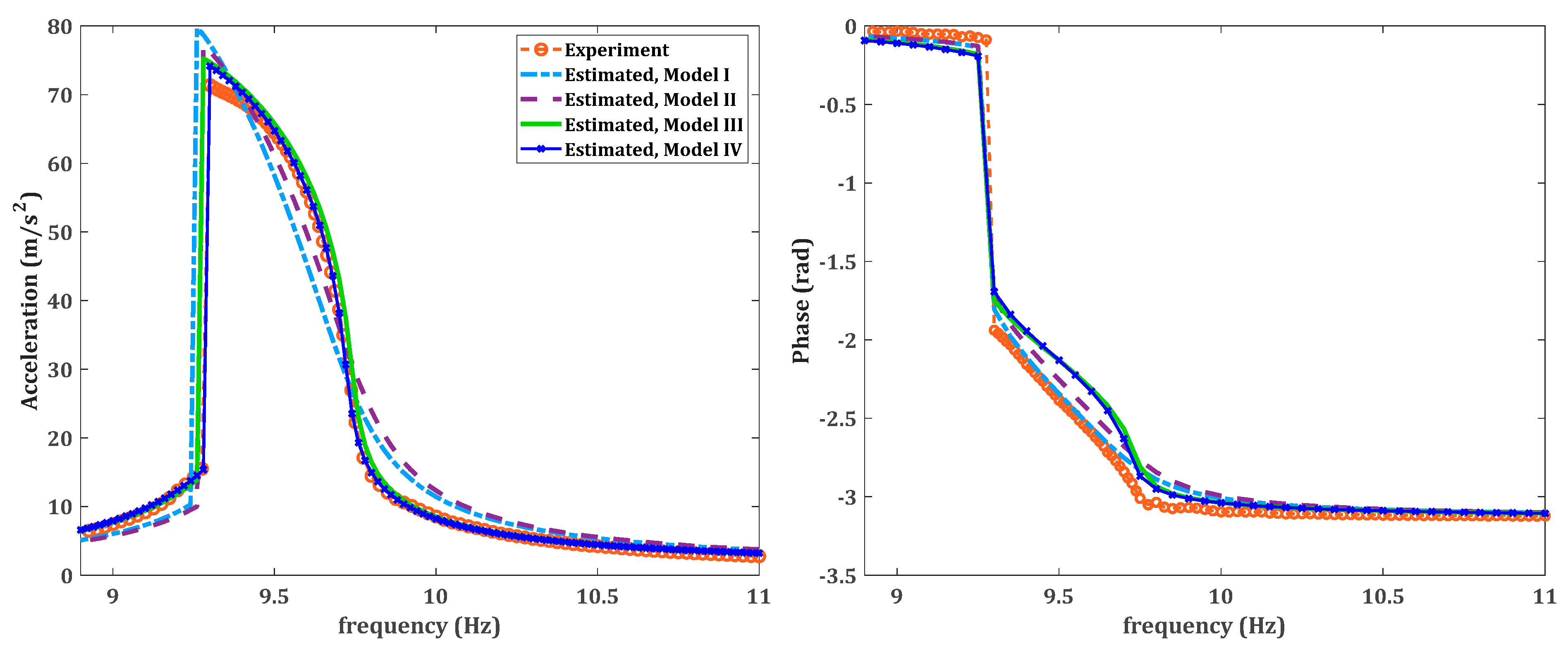
. Subsequently, the optimized parameters are used to estimate the nonlinear response of the system with the same excitation level. Figure 11 compares the measured nonlinear response, including amplitude and phase, at AM3 (25-cm away from the clamped end) with the estimated responses using all four assumed models of the nonlinear force. Figure 11 shows that the predictions from these four models are generally in good agreement with the experimental data. However, it can be seen that there is some improvement in the predictions from model III when compared to model I, while there is very little difference in the predictions between models III and IV. Based on this observation, one may conclude that because no noticeable change in the level of accuracy was achieved when the order of nonlinearity increased from model III to model IV, model III should be considered as the identified model to represent the system.

Another important problem in nonlinear system identification is assessing the validity of the model. In this example, the optimization process was performed using the response of only AM3. Therefore, in order to verify the validity of the results, the optimized parameters of model IV of the assumed nonlinear force are used to estimate the response of the nonlinear system at all three measured accelerometers, including both amplitude and phase of the acceleration. The estimated response is compared with the experimental data in Figure 12. The results illustrate a good agreement between the measured and reconstructed response and confirms the validity of the identified model.

6. Conclusions

This paper has proposed a framework for nonlinear model identification. In this framework, the nonlinear element/force was represented by a Taylor series expansion. Based on the number of terms retained in the expansion, different possible models may be chosen. An optimization-based method can be used to identify the parameters of the chosen models. The objective function of this optimization is the difference between the predicted nonlinear response and the experimental response. The predicted responses from the identified models are then compared with experimental results and one may determine how many terms should be retained in the Taylor series expansion. The proposed method is demonstrated on an experimental test case, where a nonlinear electromagnetic force is applied to the tip of a steel cantilever beam. First, the linear and nonlinear responses of the system were measured from low and high amplitude vibration tests, respectively. Euler Bernoulli beam theory is used to model the cantilever beam. The support of the beam is modelled with a spring and the effect of the mass of the support is also considered in the model. It was found that the linear model of the support is needed to predict the anti-resonances of the linear experimental responses. In the next step, four possible nonlinear models (using Taylor series expansion) were assumed for the electromagnetic force. The order of the nonlinearity in the stiffness and damping terms was increased gradually in these models. The measured nonlinear responses were used in an optimization-based identification process to estimate the unknown parameters of these models. It has been demonstrated that a nonlinear model composed of linear damping and nonlinear stiffness (including linear, quadratic, cubic, and fifth-order terms) provides excellent agreement between the predicted responses and the corresponding measured responses. In addition, it is shown that adding a quadratic nonlinear damping to the assumed nonlinear model may not lead to a significant change in the results. The identified model is capable of predicting the experimental FRFs at points which are not used in the identification. This indicated the identified model is valid.