Abstract
In this paper, the exact solution of the Timoshenko circular beam vibration frequency equation under free-free boundary conditions was determined with an accurate shear shape factor. The exact solution was compared with a 3-D finite element calculation using the ABAQUS program, and the difference between the exact solution and the 3-D finite element method (FEM) was within 0.15% for both the transverse and torsional modes. Furthermore, relationships between the resonance frequencies and Poisson’s ratio were proposed that can directly determine the elastic constants. The frequency ratio between the 1st bending mode and the 1st torsional mode, or the frequency ratio between the 1st bending mode and the 2nd bending mode for any rod with a length-to-diameter ratio, L/D ≥ 2 can be directly estimated. The proposed equations were used to verify the elastic constants of a steel rod with less than 0.36% error percentage. The transverse and torsional frequencies of concrete, aluminum, and steel rods were tested. Results show that using the equations proposed in this study, the Young’s modulus and Poisson’s ratio of a rod can be determined from the measured frequency ratio quickly and efficiently.
1. Introduction
Non-destructive testing (NDT) methods are often used to estimate the elastic properties of a material such as the dynamic elastic modulus and Poisson’s ratio. There are several types of non-destructive testing (NDT) methods available. These include ultrasonic pulse velocity methods, resonance frequency methods, and other wave propagation techniques. Material properties measured with these methods are called dynamic elastic constants. Researchers have used forced vibration and impulse vibration to measure the dynamic elastic constants of steel plates [1] as well as impact-echo resonance and Rayleigh wave velocity [2]. Kolluru et al. proposed a technique to determine the elastic material constants of a standard test cylinder using the longitudinal resonance frequencies of concrete, steel, and aluminum [3]. The ratio between the 2nd and 1st longitudinal resonance frequencies was used to determine the Poisson’s ratio for a variety of length-to-diameter ratios (L/D) and afterward the elastic modulus was estimated. Similarly, Chen and Leon proposed a method to find the two elastic constants using the 1st bending mode and the 1st torsional for rectangular prisms [4]. Nieves et al. also estimated the shear modulus and Poisson’s ratio for short cylinders using the two lowest axisymmetric natural frequencies [5]. Verification of their methods was made using various cylindrical specimens with an L/D less than 3. Wang et al. proposed a method to evaluate Poisson’s ratio of a rod with only two experimental impact-echo values (fundamental longitudinal and cross-sectional resonant frequencies). However, their methods require an for the dynamic Poisson’s ratio to be valid [6].
ASTM C215 (2014) and ASTM E1876 (2015) standards are widely used to determine the dynamic elastic modulus using the fundamental resonance frequency. The equations provided in these standards were formulated by simplifying the free-free vibration solution of a Timoshenko beam with the effects of shear and rotational inertia reduced to a simple correction constant. However, the value of the elastic modulus cannot be directly calculated without knowing the material’s Poisson’s ratio. Therefore, in order to calculate the dynamic modulus and Poisson’s ratio, a lengthy iteration process is needed.
In this paper, the exact solution of the Timoshenko beam vibration frequency equation under free-free boundary conditions was determined. The fundamental transverse and torsional frequencies were used to determine the dynamic elastic modulus and Poisson’s ratio of rods with an L/D ≥ 2. Then, relationships between the resonance frequencies and Poisson’s ratio were proposed that can directly determine the elastic modulus and the Poisson’s ratio, simultaneously without the need for iteration, using the frequency ratio between the 1st bending mode and the 1st torsional mode, or the frequency ratio between the 2nd bending mode and the 1st bending mode.
2. Analysis
For a homogenous and isotropic material, the Timoshenko beam vibration equation can be expressed as follows:
In the equation, is the transverse displacement; t is time; is a shape factor that depends only on Poisson’s ratio; G is the shear modulus; E is the Young’s modulus; I is the moment of inertia of the cross-section; ρ is the mass density; and m is the mass per unit length. In Timoshenko’s publication [7], a shape factor of was assumed for a circular cross-section. However, Hutchinson derived more accurate shape factors for a variety of geometries which match more closely with experimental results [8]. In this paper, Hutchinson’s shape factor, Equation (2), was used to calculate the shape factor for a circular cross-section:
For a rod with free-free boundary conditions, the following can be applied:
Using these boundary conditions for a nontrivial solution, the frequency equation can be written as follows [9,10]:
where , , and A is the cross-sectional area; α and β represent the eigenvalues of the frequency equation. The eigenvalues α and β can be expressed as follows:
In this paper, a MATLAB program was used to solve for the eigenvalues of the frequency equation. The natural frequencies (Hz) can be expressed using the eigenvalues [11]:
Let i = 1 to obtain the 1st bending mode and i = 2 for the 2nd bending mode.
2.1. Finite Element Analysis
Dynamic analysis using the 3-D finite element method (FEM) was carried out and compared to the exact solution for the transverse and torsional modes of a rod. The density was assumed to be 2400 . Six different sets of elastic modulus and Poisson’s ratio were used in the FEM simulations as shown in Table 1.

Table 1.
Elastic modulus and Poisson’s ratio assumed in the finite element method (FEM).
A total of 199,950 elements of 2.0 mm (0.08 in) cubes, 8-node linear brick with reduced integration and hourglass control elements (C3D8R) from the ABAQUS program were utilized. A 75 mm (diameter) × 300 mm (length) rod was modeled as a free-free beam. The 1st and 2nd bending modes as well as the 1st torsional mode are shown in Figure 1.
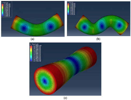
Figure 1.
Mesh of 75 mm (D) × 300 mm (L) rod: (a) 1st bending mode: 2101.5 Hz, (b) 2nd bending mode: 4910.6 Hz, (c) 1st torsional mode: 3622.1 Hz.
A comparison between the FEM and the analytical solutions is shown in Table 2. Results show that the percent error for all the cases is less than 0.13%. This indicates that the elastic modulus and Poisson’s ratio obtained from the roots of the Timoshenko beam frequency equation in the analysis section above is accurate and the 1st free-free torsional mode from the Euler–Bernoulli beam solution, , is also close to exact, where R is the ratio between the polar moment of inertia and the equivalent moment of inertia, for a rod R = 1.0. Since the FEM usually requires large amounts of computations using commercial software, it would be more efficient to use the analytical solutions to determine the transverse and torsional vibration frequencies.
Table 2.
Comparison of the FEM and the analytical solutions.
2.2. Frequency Ratio Analysis
The ratio between the fundamental torsional frequency and the fundamental transverse frequency, , can be expressed as follows [11]:
where is the fundamental torsional frequency (Hz) and is the 1st fundamental transverse frequency (Hz). Using the roots of the Timoshenko frequency equation, Equation (3), and the solution for the torsional mode, the frequency ratio, , is expressed as Equation (7):
Equation (7) was evaluated for a variety of Poisson’s ratios and rod dimensions as shown in Figure 2. From Figure 2, a linear relationship between the Poisson’s ratio, , and the ratio can be observed. A clear linear trend can be seen after normalizing the frequency ratio,, with at v = 0 as shown in Figure 2c. It was found that the slope of the line and the y-intercept are independent of the elastic modulus and the mass density. The frequency ratio, , only depends on the diameter and the length of the rod as shown in Equation (7). Hence, the ratio can be expressed as Equation (8):
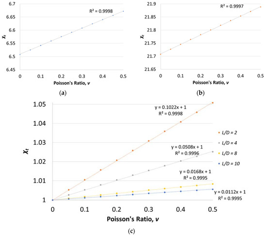
Figure 2.
Relationship between and Poisson’s ratio with different rod dimensions (diameter × length): (a) 100 mm × 400 mm, (b) 20 mm × 160 mm, and (c) normalized for different L/D ratios (L/D = 2, 4, 8, and 10).
The Poisson’s ratio can then be calculated using the equation below:
Furthermore, after knowing Poisson’s ratio, the elastic modulus can be determined using the experimental torsional frequency with Equation (10):
The values of and for different specimen dimensions were found by calculating for different length/diameter ratios as well as varying Poisson’s ratio (shown in Appendix A). The constant was found by calculating when Poisson’s ratio was equal to zero. The calculated values for are shown in Table 3. A similar procedure was carried out to determine . After plotting , the slope of the best-fit line was used to find . Table 3 shows the calculated value of for different length/diameter (L/D) ratios.
Table 3.
Values of for different length/diameter ratios.
As shown in Figure 3 and Figure 4, polynomials can be used to express the values of . Although only nine L/D points are shown in Table 3, a total of 97 L/D data points were used to find the best-fit polynomials. Due to the wide range of , shown in Figure 3, a single polynomial will have a 3% difference between the estimated values and the theoretical values found using Equation (8) when . Therefore, to reduce the difference to less than 0.06%, two polynomials (sixth-order) are needed to express for two separate intervals, Equations (11) and (12).
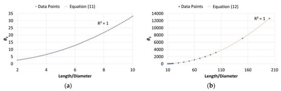
Figure 3.
Plot of B1 versus the length/diameter ratio: (a) and (b) .
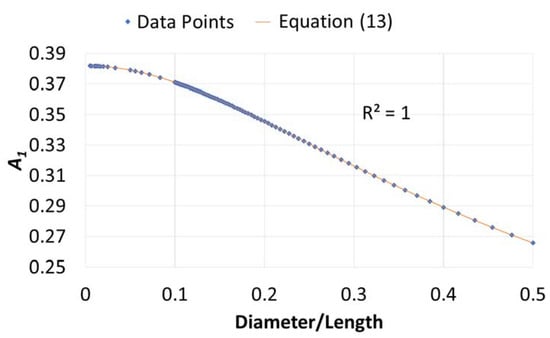
Figure 4.
Plot of A1 versus diameter/length (D/L) ratio.
For ,
For ,
Unlike B1, only a single polynomial expression is needed for A1. Equation (13) was found from the best-fit curve shown in Figure 4. Equation (13) can be used to obtain for any diameter/length (D/L) ratio:
Although the method presented above can be used to determine the dynamic elastic constants easily and quickly, it has two disadvantages. First, it requires a precise measurement of the torsional mode which is difficult to excite in a cylindrical specimen [6,12]. Additionally, it requires two separate experimental tests. Therefore, it would be beneficial to develop a method based on only the transverse bending modes which can be measured simultaneously and accurately. Similar to , the ratio between the 2nd bending mode and the 1st bending mode was used to directly calculate Poisson’s ratio and the dynamic elastic modulus.
The ratio between the 2nd and 1st fundamental transverse frequencies, , can be expressed with the following relationship:
where is the 2nd fundamental transverse frequency (Hz). and are the roots from the frequency equation, shown in Equation (3), for the 1st and the 2nd bending modes. For a very slender rod, the relationship shown in Equation (15) can be derived to express for a Euler–Bernoulli rod with free-free boundary conditions:
However, for the vibration of a non-slender rod, can only be expressed with the roots of the Timoshenko frequency equation using Equation (3). Hence, Equation (14) was evaluated for a variety of Poisson’s ratios and rod dimensions as shown in Figure 5. From Figure 5, a slightly parabolic relationship between the Poisson’s ratio, v, and the ratio can be observed. A clear trend can be seen after normalizing the frequency ratio,, with at v = 0 as shown in Figure 5c. The y-intercept, , corresponds to the value of when v = 0. It was found that the frequency ratio, , is independent of the elastic modulus and the mass density, and only depends on the roots of Equation (3). Hence, the ratio can be expressed as Equation (16):
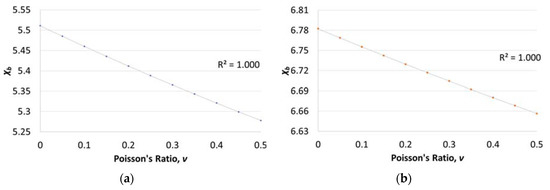
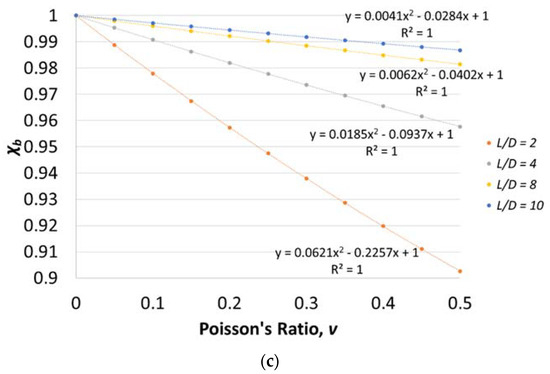
Figure 5.
Relationship between and Poisson’s ratio with different rod dimensions (diameter × length): (a) 100 mm × 400 mm, (b) 20 mm × 160 mm, and (c) normalized for different L/D ratios (L/D = 2, 4, 8, and 10).
are the coefficients of the second-order polynomial describing the relationship between and Poisson’s ratio. Table 4 shows the calculated values of , , and due to different Poisson’s ratio and length/diameter (L/D). As expected, as the L/D ratio becomes very large, the values of and approach 4.73 and 7.853. They are the same values shown in Equation (15) and correspond to a Euler–Bernoulli beam. For a very slender rod (L/D = 200), is no longer dependent on Poisson’s ratio and approaches a constant value.
Table 4.
Calculation of , , and for different length/diameter ratios.
The Poisson’s ratio can then be calculated using the equation below:
Therefore, Poisson’s ratio can be readily calculated using the experimentally measured transverse vibration frequencies, and . Furthermore, after knowing Poisson’s ratio, the elastic modulus can be determined using the first bending mode as shown in Equation (18). To find , one can use Equations (7) and (8) and the calculated Poisson’s ratio from Equation (17). Hence, the elastic modulus can be calculated directly as follows:
The equation can also be used to determine the first bending mode solely from the dimensions of the rod and assumed elastic constants without solving the Timoshenko frequency equation. The values of , , and for different specimen dimensions were found by calculating for different length/diameter ratios as well as varying Poisson’s ratio (shown in Appendix A). It is noted from Equation (14) that the frequency ratio is only dependent on the roots of the Timoshenko frequency equation and is independent of the elastic modulus and mass density. Therefore, any set of material properties would produce the same values of , , and . The values of and its derived , , and shown in this paper are only applicable to the 1st and 2nd bending modes of a Timoshenko rod with free-free boundary conditions. The constant was found by calculating when Poisson’s ratio was equal to zero. The calculated values for are shown in Table 5.
Table 5.
The values of , , and for different length/diameter ratios.
A similar procedure was carried out to determine the coefficients and . The transverse modes were determined using Poisson’s ratio ranging from 0.0 to 0.5 in increments of 0.05. After plotting , the best-fit second-order polynomial was used to find and . The coefficient of determination, , was above 0.999 for all the cases. Table 5 shows the calculated values for different specimen dimensions. Unlike , the coefficients decrease when the length/diameter ratio is enlarged. As the rod gets longer, the values of and approach zero, indicating that the rod behaves more like a Euler–Bernoulli slender rod. For larger length/diameter ratios (L/D > 20), approaches a constant value equal to only .
As shown in Figure 6, Figure 7 and Figure 8, the three coefficients can be estimated using polynomial equations, and to increase the accuracy of the proposed method, two intervals are specified for . A total of 97 L/D data points were used to determine the polynomials. The proposed equations can be used to find the coefficients for any and allows for the calculation of the elastic constants after knowing the 1st and 2nd bending modes as well as the rod’s dimensions. The sixth-order polynomials were found to have a maximum percent difference of 0.12% with the theoretical values. On average, the percent difference was 0.01% indicating that the sixth-order polynomials can be used adequately to estimate the coefficients.
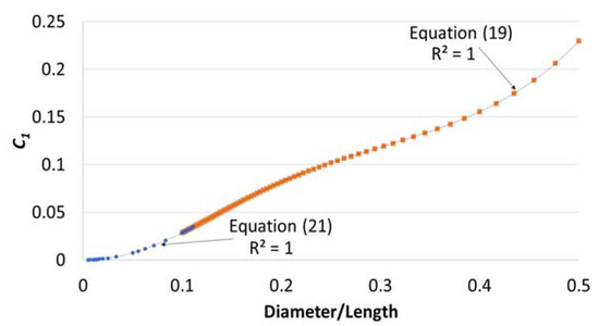
Figure 6.
Plot of C1 versus the diameter/length (D/L) ratio.
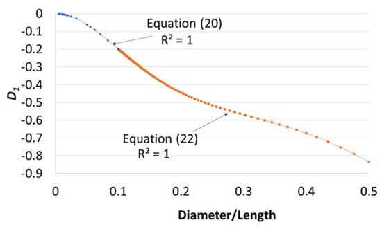
Figure 7.
Plot of D1 versus the diameter/length (D/L) ratio.
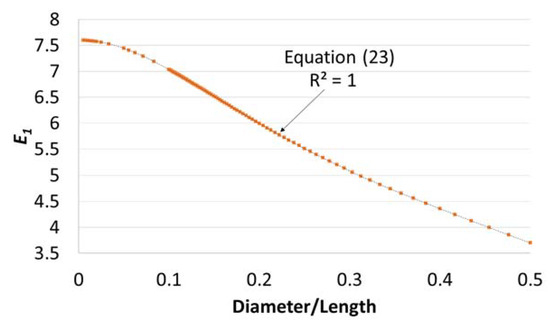
Figure 8.
Plot of E1 versus the diameter/length (D/L) ratio.
For
For
A single sixth-order polynomial can be used to estimate . The equation is shown below:
As an example, the FEM was performed for a steel rod with an assumed elastic modulus, Poisson’s ratio, and density of 200 GPa, 0.3, and 7750 , respectively. The values of and were obtained from Equations (11)–(13), whereas were obtained using Equations (19)–(23). Table 6 shows that the 1st and 2nd bending modes as well as the 1st torsional mode frequency calculated using Equations (9), (10), and (16) compare closely with the FEM results with a maximum difference of 0.36%.
Table 6.
Steel rod with different length/diameter ratios.
3. Experiments
Aluminum, steel, and concrete rods with different length/diameter ratios were experimentally tested to validate the proposed methods. The density and specimen dimensions can be found in Table 7. It should be noted that the dimensions of the rods must be measured accurately for a correct estimation of the elastic modulus and Poisson’s ratio.
Table 7.
Material properties of the rods.
The impact resonance frequency method was used to measure the fundamental transverse and torsional modes. Figure 9 shows the instruments and specimens used in the experiment. The rods were suspended with soft flexible rubber tubing placed at approximately 0.15L to allow free vibration in the fundamental transverse and torsional modes as shown in Figure 9. The accelerometer was attached to the specimen centered at 0.55L from the edge of the specimen using a hot glue adhesive. The torsional frequency was also tested for each rod. The supports were kept at the same location as the transverse mode experiment. The accelerometer was placed with hot glue adhesive on a rigid metal tab which was located 0.223L from the edge of the specimen. A tangential impact was made using another metal tab located 0.13L from the other edge. A schematic of the torsional mode testing can be found in ASTM C215. For each test, the acceleration time history was plotted on a LabView waveform analyzer. Using fast Fourier transform (FFT), the time domain was converted to the frequency domain.
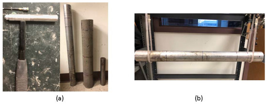
Figure 9.
Picture of experiment: (a) Impact hammer, accelerometer, and specimens; (b) Experimental setup.
Experimental Data
Typical acceleration time histories for the impact and response before and after performing the FFT are shown in Figure 10 and Figure 11. The excitation frequency range for the transverse and torsional impact is approximately 5000 Hz. To find the peak frequency, the frequency response function, which is the ratio between the output response and the input excitation force in the frequency domain, was calculated [13]. Four peaks can be seen in the output response; these peaks correspond to the first four fundamental bending modes. In this study, only the 1st and 2nd bending modes were analyzed; however, the 3rd and 4th bending modes could be used as verification of the measured elastic constants.
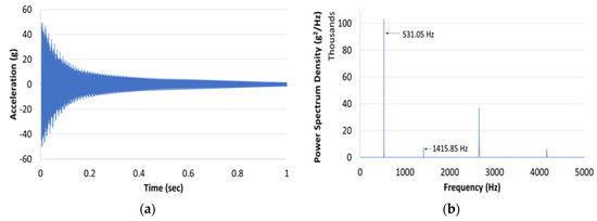
Figure 10.
(a) Typical acceleration time history and (b) Typical response power spectrum (transverse mode).
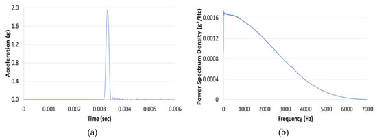
Figure 11.
(a) Typical impact loading time history and (b) Typical impact power spectrum (transverse mode).
Similarly, Figure 12 and Figure 13 present the typical acceleration time histories and the frequency response function for the torsional mode. A clear peak can be seen in all the specimens.
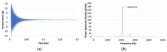
Figure 12.
(a) Typical acceleration time history and (b) Typical response power spectrum density (torsional mode).
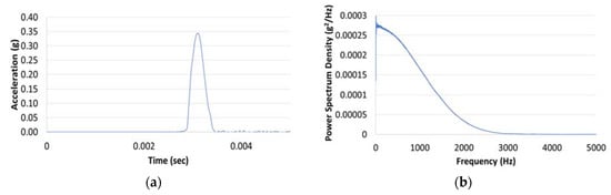
Figure 13.
(a) Typical impact loading time history and (b) Typical impact power spectrum (torsional mode).
Table 8 presents the average measured frequencies for the fundamental transverse and torsional frequencies of the three rods. The average value was determined from at least four tests. The sampling frequency for both impact force and acceleration response was 25.6 kHz, and the resolution of the measured frequencies was increased to 0.25 Hz using a signal processing technique.
Table 8.
Calculated properties of the aluminum, steel, and concrete rods.
4. Data Analysis
The values for , , , and can be obtained for each rod specimen using their respective L/D ratio. Using Equations (9) and (17), the Poisson’s ratio for the three rods was calculated and is shown in Table 8. The calculated values for the dynamic elastic modulus using Equations (10) and (18) are also shown in Table 8. Table 8 shows a comparison between Method 1 and Method 2. Method 1 uses to calculate Poisson’s ratio and elastic modulus. As expected, Method 2, which uses the 1st and 2nd bending modes, produces more reasonable elastic constants. This is mainly due to the inaccuracy of the experimental torsional mode frequency. Note, the largest difference occurs in the Poisson’s ratio while the elastic modulus for both methods are almost identical.
Sensitivity Analysis
In this study, the diameter and length of the specimens were measured with a resolution of 0.01 mm, while the mass had a resolution of 0.01 kg. A sensitivity analysis of the proposed methods was conducted using the experimental resolution. The experimental frequencies were measured with a resolution of 0.25 Hz, which was achieved using a signal processing technique. It was found that Poisson’s ratio and the elastic modulus had a maximum deviation of 0.3 ± 0.001 and 218.91 ± 0.2 GPa, respectively, when changing the diameter or length by 0.01 mm. Therefore, it is recommended to at least have a resolution of 0.1 mm in order to achieve an accuracy of Poisson’s ratio with ±0.01 deviation. It was also found that a mass change of 0.01 kg can influence the elastic modulus by ±0.5 GPa. Furthermore, if only a 0.25 Hz frequency resolution is obtainable, the estimated Poisson’s ratio can have a large deviation of ±0.05 when a specimen has a large L/D like the aluminum specimen (L/D = 11.6). This is because, as shown in Figure 5 and Table 4, Poisson’s ratio is not sensitive to the change of the bending frequency ratio when L/D becomes large. During the experiment, the concrete and steel rods both showed high accuracy in the measurement of Poisson’s ratio using the bending modes as displayed in Table 9. However, since the aluminum rod has an L/D = 11.6, a frequency resolution of ±0.05 Hz was used to reduce the Poisson’s ratio deviation to ±0.009. For an accurate measurement of the Poisson’s ratio, it is recommended that an L/D 6 be used when using .
Table 9.
Sensitivity analysis of the aluminum, steel, and concrete specimens.
5. Discussion
The frequency ratio between the first torsional mode and the first bending mode, , was found to be linearly proportional to the Poisson’s ratio with a slope, , and a y-intercept, , whereas the frequency ratio between the first two bending modes, , was slightly parabolic with coefficients , and . It was found that the constants , , , , and depend only on the dimensions of the specimen and can be tabulated for different specimen sizes. Values for , , , , and at different length/diameter ratios were found, allowing the use for any rod dimensions. As the length/diameter ratio increased, the value of could be ignored and approached to a constant. In other words, is independent of Poisson’s ratio at very large length/diameter ratios. Likewise, as the length/diameter increases, the values of and approach to zero, and approaches a constant value of 7.598. Equations for the elastic modulus, E, and Poisson’s ratio, v, were proposed in this paper using the tabulated values of , allowing for a quick calculation of both E and v. The proposed methods do not require any iterations to solve for the material constants. Results show that, using the equations proposed in this study, the Young’s modulus and Poisson’s ratio of a rod can be determined from the measured frequency ratio quickly and efficiently.
6. Conclusions
This paper presents a method to calculate Poisson’s ratio and dynamic elastic modulus using experimentally measured transverse and torsional modes. The method is based on the exact solution to the frequency equation for a Timoshenko rod under free-free boundary conditions. The finite element method using the ABAQUS program was shown to match the exact solution with less than 0.15% error for both the transverse and torsional modes. Equations for the elastic modulus, E, and Poisson’s ratio, v, were proposed in this paper using the frequency ratio values, allowing for a quick calculation of both E and v. The frequency ratio between the first bending mode and the first torsional mode or the frequency ratio between the first bending mode and the second bending mode for any rod with a length-to-diameter ratio of can be directly estimated using the proposed equations. The proposed method does not require any iterations to solve for the material constants and can be used to calculate the elastic constants of rods with different dimension sizes. The proposed equations were used to verify the elastic constants of a steel rod with less than 0.36% error percentage, and the equations were also used to measure elastic constants of three rods with different material properties (aluminum, steel, and concrete) using simple impact vibration. It was found that the torsional mode is more difficult to excite and not as reliable as the bending modes, whereas a more accurate measurement can always be obtained from using the 1st and 2nd bending modes which were measured simultaneously.
Author Contributions
Conceptualization, G.L. and H.-L.C.; Methodology, G.L. and H.-L.C.; Validation, G.L.; Writing—Original Draft Preparation, G.L.; Writing—Review and Editing, H.-L.C.
Funding
This research was partially funded by the WVDOH/FHWA research project number [RP#312].
Acknowledgments
The authors acknowledge the support provided by the West Virginia Transportation Division of Highways (WVDOH) and the Federal Highway Administration (FHWA) for the research project WVDOH RP#312. Special thanks are extended to our project monitors, Mike Mance, Donald Williams, and Ryan Arnold of WVDOH.
Conflicts of Interest
The authors declare no conflict of interest.
Appendix A
Values of frequency ratios and and values of the first two roots ( of the Timoshenko frequency equation for different length/diameter ratios (L/D) at various Poisson’s ratios.
Table A1.
Values of and for different length/diameter ratios at various Poisson’s ratios
Table A1.
Values of and for different length/diameter ratios at various Poisson’s ratios
| Length/Diameter | Poisson’s Ratio | ||||
|---|---|---|---|---|---|
| 2 | 0 | 3.948 | 5.476 | 2.599 | 3.699 |
| 0.1 | 3.938 | 5.431 | 2.626 | 3.617 | |
| 0.2 | 3.928 | 5.389 | 2.653 | 3.541 | |
| 0.3 | 3.919 | 5.348 | 2.679 | 3.469 | |
| 0.4 | 3.909 | 5.309 | 2.705 | 3.402 | |
| 0.5 | 3.900 | 5.271 | 2.731 | 3.338 | |
| 3 | 0 | 4.275 | 6.336 | 4.256 | 4.827 |
| 0.1 | 4.267 | 6.305 | 4.288 | 4.768 | |
| 0.2 | 4.259 | 6.275 | 4.319 | 4.712 | |
| 0.3 | 4.252 | 6.246 | 4.349 | 4.658 | |
| 0.4 | 4.244 | 6.218 | 4.379 | 4.607 | |
| 0.5 | 4.237 | 6.191 | 4.408 | 4.558 | |
| 4 | 0 | 4.439 | 6.801 | 6.508 | 5.511 |
| 0.1 | 4.433 | 6.776 | 6.542 | 5.460 | |
| 0.2 | 4.427 | 6.753 | 6.576 | 5.412 | |
| 0.3 | 4.422 | 6.730 | 6.608 | 5.365 | |
| 0.4 | 4.417 | 6.708 | 6.640 | 5.321 | |
| 0.5 | 4.411 | 6.686 | 6.672 | 5.278 | |
| 5 | 0 | 4.530 | 7.088 | 9.372 | 5.992 |
| 0.1 | 4.526 | 7.068 | 9.408 | 5.948 | |
| 0.2 | 4.522 | 7.049 | 9.443 | 5.906 | |
| 0.3 | 4.518 | 7.031 | 9.477 | 5.866 | |
| 0.4 | 4.514 | 7.013 | 9.510 | 5.827 | |
| 0.5 | 4.510 | 6.996 | 9.543 | 5.790 | |
| 8 | 0 | 4.645 | 7.496 | 21.707 | 6.782 |
| 0.1 | 4.643 | 7.485 | 21.745 | 6.755 | |
| 0.2 | 4.641 | 7.475 | 21.782 | 6.729 | |
| 0.3 | 4.639 | 7.465 | 21.818 | 6.704 | |
| 0.4 | 4.637 | 7.455 | 21.853 | 6.680 | |
| 0.5 | 4.636 | 7.446 | 21.888 | 6.656 | |
| 10 | 0 | 4.675 | 7.613 | 33.073 | 7.035 |
| 0.1 | 4.673 | 7.606 | 33.111 | 7.016 | |
| 0.2 | 4.672 | 7.598 | 33.149 | 6.997 | |
| 0.3 | 4.671 | 7.591 | 33.185 | 6.978 | |
| 0.4 | 4.669 | 7.584 | 33.221 | 6.960 | |
| 0.5 | 4.668 | 7.577 | 33.256 | 6.943 | |
| 20 | 0 | 4.716 | 7.789 | 127.726 | 7.441 |
| 0.1 | 4.715 | 7.786 | 127.766 | 7.435 | |
| 0.2 | 4.715 | 7.784 | 127.804 | 7.429 | |
| 0.3 | 4.715 | 7.782 | 127.841 | 7.423 | |
| 0.4 | 4.714 | 7.780 | 127.877 | 7.418 | |
| 0.5 | 4.714 | 7.778 | 127.913 | 7.412 | |
| 50 | 0 | 4.728 | 7.843 | 790.220 | 7.572 |
| 0.1 | 4.728 | 7.842 | 790.259 | 7.571 | |
| 0.2 | 4.728 | 7.842 | 790.298 | 7.570 | |
| 0.3 | 4.728 | 7.842 | 790.335 | 7.569 | |
| 0.4 | 4.728 | 7.841 | 790.372 | 7.568 | |
| 0.5 | 4.727 | 7.841 | 790.408 | 7.568 | |
| 100 | 0 | 4.729 | 7.851 | 3156.257 | 7.592 |
| 0.1 | 4.729 | 7.850 | 3156.297 | 7.592 | |
| 0.2 | 4.729 | 7.850 | 3156.335 | 7.591 | |
| 0.3 | 4.729 | 7.850 | 3156.373 | 7.591 | |
| 0.4 | 4.729 | 7.850 | 3156.409 | 7.591 | |
| 0.5 | 4.729 | 7.850 | 3156.446 | 7.591 |
References
- Alfano, M.; Pagnotta, L. A non-destructive technique for the elastic characterization of thin isotropic plates. NDT E Int. 2007, 40, 112–120. [Google Scholar] [CrossRef]
- Medina, R.; Bayón, A. Elastic constants of a plate from impact-echo resonance and Rayleigh wave velocity. J. Sound Vib. 2010, 329, 2114–2126. [Google Scholar] [CrossRef]
- Kolluru, S.; Popovics, J.; Shah, S. Determining Elastic Properties of Concrete Using Vibrational Resonance Frequencies of Standard Test Cylinders. Cement Concr. Aggreg. 2000, 22, 81–89. [Google Scholar]
- Chen, H.-L.; Leon, G. Direct Determination of Dynamic Elastic Modulus and Poisson’s Ratio of Rectangular Timoshenko Prisms. J. Eng. Mech. in press. [CrossRef]
- Nieves, F.J.; Gascón, F.; Bayón, A. Estimation of the elastic constants of a cylinder with a length equal to its diameter. J. Acoust. Soc. Am. 1998, 104, 176–180. [Google Scholar] [CrossRef]
- Wang, J.-J.; Chang, T.-P.; Chen, B.; Wang, H. Determination of Poisson’s Ratio of Solid Circular Rods by Impact-Echo Method. J. Sound Vib. 2012, 331, 1059–1067. [Google Scholar] [CrossRef]
- Timoshenko, S. Vibration Problems in Engineering, 2nd ed.; D. Van Nostrand Co.: New York, NY, USA, 1937. [Google Scholar]
- Hutchinson, J.R. Shear Coefficients for Timoshenko Beam Theory. J. Appl. Mech. 2000, 68, 87–92. [Google Scholar] [CrossRef]
- Goens, E. Uber die Bestimmung des Elastizitätsmoduls von Stäben mit hilfe von Biegungsschwingungen. Annalen Der Physik. 1931, 403, 649. [Google Scholar] [CrossRef]
- Chen, H.-L.; Kiriakidis, A.C. Nondestructive Evaluation of Ceramic Candle Filter with Various Boundary Conditions. J. Nondestruct. Eval. 2005, 24, 67–81. [Google Scholar] [CrossRef]
- Huang, T.C. The Effect of Rotatory Inertia and of Shear Deformation on the Frequency and Normal Mode Equations of Uniform Beams with Simple End Conditions. J. Appl. Mech. 1961, 28, 579–584. [Google Scholar] [CrossRef]
- Standard Test Method for Fundamental Transverse, Longitudinal, and Torsional Resonant Frequencies of Concrete Specimens; ASTM International: West Conshohoken, PA, USA, 2014.
- Chen, H.-L. “Roger”, Kiriakidis Alejandro C., Stiffness Evaluation and Damage Detection of Ceramic Candle Filters. J. Eng. Mech. 2000, 126, 308–319. [Google Scholar] [CrossRef]
© 2019 by the authors. Licensee MDPI, Basel, Switzerland. This article is an open access article distributed under the terms and conditions of the Creative Commons Attribution (CC BY) license (http://creativecommons.org/licenses/by/4.0/).