2D Flameballs: An Enhanced Classification Based on Soliton Theory

Abstract

In a Hele-Shaw cell, unconventional fragmented flame propagation occurs for Peclet numbers less than 15. Until now, the regimes arising were organized in a simple taxonomy. Here, we endeavor to classify our experiments in view of the Theory of Solitons, a part of Synergetics discipline. This approach allows us to recognize new general patterns previously unidentified. Furthermore, this permits us to identify a much richer variety of topologies and typologies of regimes than initially thought.

1. Introduction

In this paper, we study flames propagating in a thin slit between two parallel plates, so-called Hele-Shaw geometry. During the classification of continuous flame propagation regimes in a Hele-Shaw cell geometry, a new class of fragmented flames in gaseous combustion appeared below the conventional quenching limit at $Pe<40$ [1]. In such narrow cavities, when the typical sizes of the gap is on the order of millimeters, the Reynolds number remains modest ($Re<100$), and the propagation regime is laminar [2]. This is accompanied by intense heat and momentum losses, typically characterized by a low Peclet number. Due to a local extinction at the Peclet numbers $30>Pe>15$, the flame starts to be fragmented. The small tongues of continuous fractal flame are zigzagging, escaping the pockets of unburned material [3]. The fraction of unburned material remains insignificant (less than 10%). Then, following the findings of [4], at a Peclet number less than 15 ($15>Pe>5$), a variety of singular flame propagation regimes appear, a phenomenon discovered by Veiga et al. [5]. The regime is characterized by flame front disintegration in the form of a set of tiny flamelets separated by a mass of non-burned material [5]. This discontinuous front is not unique. It shows a multiplicity of morphologies and regimes that mostly remain unexplained.

The dendritic patterns of [5] have occurred before in combustion, but only in studies utilizing solid fuels. Observations occurred for smoldering in a Hele-Shaw cell [6,7,8]. The patterns were attributed to the mass diffusivity of the deficient component, the oxidizer. Apparently, the deficit of air was compensated by diffusion from surrounding areas creating reactive solitary waves [9] in which heat losses counteract enhanced air diffusion sustaining a local combustion process.

For a further contextualization of this research, we need to mention the theoretical/numerical studies on combustion in enclosures by Kurdyumov and Matalon [10]. From their initial formulation, their model was subsequently refined. Notably it accounts for heat losses [11] and buoyancy forces [12]. Using this methodology, Martinez-Ruiz and his co-authors [13] reproduced mono- and bi-cellular patterns in a 2D configuration [14]. Their results of [13] even reproduce the flame front splitting and constitute an analogue to the patterns previously found in Kagan et al. [15].

It can be stated from [13,14] that a low Lewis number is a necessary condition to obtain unconventional propagation. Still, this condition is not a sufficient one. The statistical exploitation of the experimental data gathered by [5] was carried out by Yanez et al. [4]. There, it was concluded that heat losses are causing the unconventional propagation. Also notably, statistical evidence showed that the Lewis number was definitely not the effect triggering the flame fragmentation.

As can be inferred from the paragraphs above, most of the previous studies were devoted to the explanation of the phenomenon. The reasoning was done in terms of the physical mechanism determining the phenomenon, or regarding the numerical reproduction of the experiments. Let us now turn our attention to the topologies of the flames resulting from the experiments.

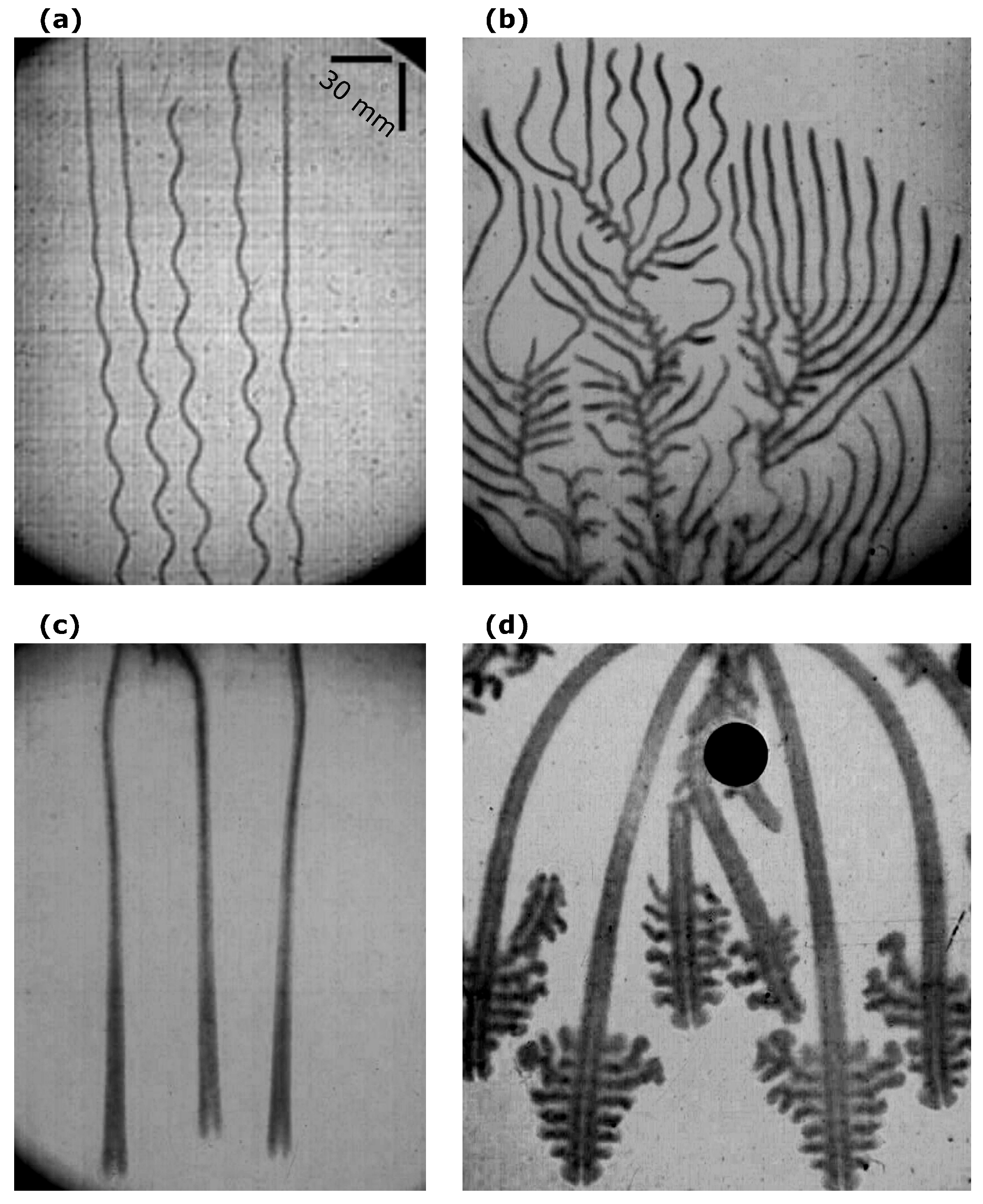
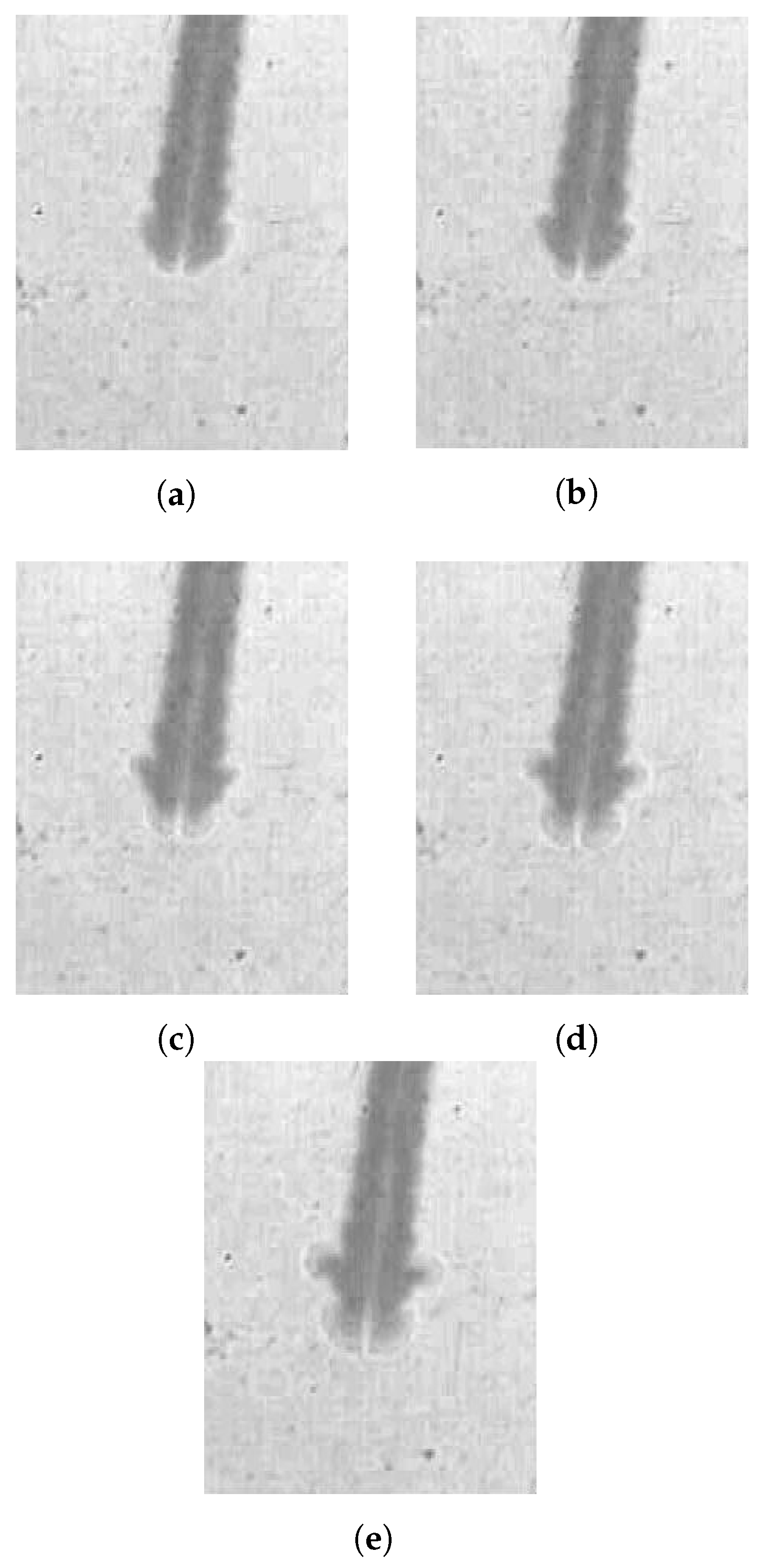
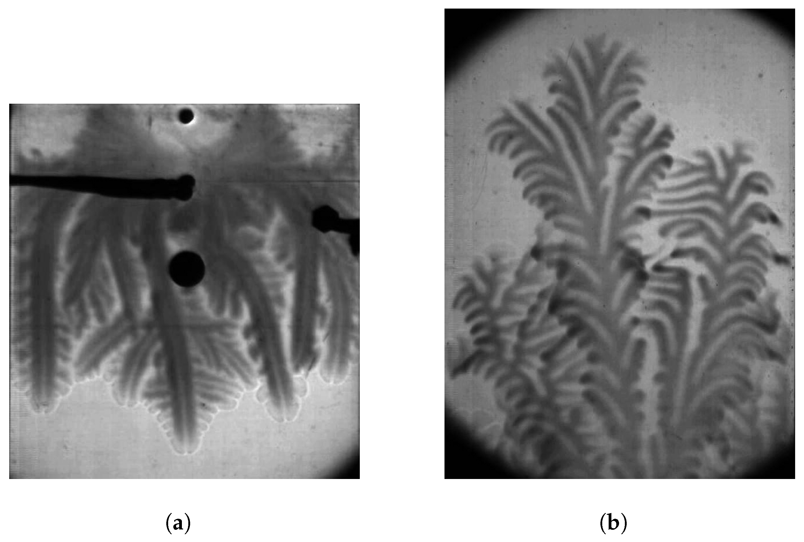
In Figure 1, we observe shadowgraphs taken in our Hele-Shaw cell [5]. Dark traces are created by steam, the product of combustion, and represent the paths of the flamelets. Originally, the regimes arising in unconventional propagation have been categorized into four typologies [4]: (a) Mono-cellular; (b) Mono-cellular with branching; a singular mono-cellular front may bifurcate cyclically into several independent mono-cellular fronts producing menorah-like structures; (c) Bi-cellular; (d) Bi-cellular with branching; when two-headed fronts also bifurcate cyclically, producing palm-tree structures.

An alternative classification has been proposed by Moskalev et al. [16]. For their horizontal experiments and considering the morphology of the front, these authors provide three categories: (a) ray-like traces, for propagation following a more or less straight line; (b) dendrite-like patterns, if there is splitting of the structures; (c) quasi-homogeneous track, when a continuous front is observed. Alternatively, and based on the behavior of the front, a second taxonomy is proposed: (i) self-extinguishing; (ii) self-sustained; (iii) self-branching.

The information gathered above allows us to conclude that the classification has been until now quite superficial. Note that the taxonomy involves few categories, and these can hardly account for the multiplicity of regimes that one observes in the photographs coming from the experiments.

This is not surprising. In our opinion, the exhaustive experimental research of the phenomenon at hand is still unfinished. For example, even the determination of the conditions in which each of the propagation regimes occur is still incomplete. Furthermore, it cannot be excluded that some propagation regimes remain unobserved. The influence of each of the parameters (thickness, reactivity, …) or dimensionless numbers (Pe, Re, …) in the determination of the type of unconventional regime is also an arcane. The only established frontier [4] is the one of $Pe<15$, and it concerns only unconventional propagation with all regimes confounded. The explanation of the flame topology, splitting and merging of the dendritic flame does not exist.

In addition to the lack of knowledge, the classification efforts have suffered from a more systematic issue. They have not been based on the theory of Synergetics [17]. The latter is a discipline pioneered by Haken [18], which is devoted to the understanding of self-organization and pattern formation in systems far from equilibrium. The pertinence of such an approach seems to us utterly justified by regarding the systemic patterns contained in Figure 1.

Synergetics is interdisciplinary. Therefore the domain of phenomena analyzed by these science is wide. Here we concentrate in results applying to reaction-diffusion systems, a topic pioneered by Turing [19]. In this sense, note that a reaction-diffusion system has been utilized by us in [20,21] to determine the conditions of steady propagation of a single flamelet. There is ample description of reaction-diffusion systems in synergetic science, see [22]. One of the notable structures appearing in such systems is the isolated waves, that will be discussed in Section 2.1.

With the considerations outlined in the previous paragraphs, we will devote this paper to describe and classify in a more complex manner the intricate typologies of the topologies appearing in our experiments [5,23]. To achieve these goals, our paper is structured as follows. In Section 2, we establish the connection between the formulation of our previous theoretical work [24] and the general one that is found in the literature on solitons [25]. We then classify our reaction-diffusion system accordingly. By identifying our specific soliton type in this manner, we can infer the experimental phenomena we may expect to find. In Section 3, we try to identify these patterns within the experiments. Finally, in the conclusion we summarize the observations to provide an expanded classification framework.

To finalize this section, we want to state explicitly that the classification we are proposing, with the identification of phenomena by mere observation, is not sustained by mathematical treatment. Therefore, most rigorous readers may prefer to consider this paper, and particularly Section 3, as a mere collection of non-assorted pictures, that describes nevertheless an incontrovertible reality.

2. Interpretation of the Experiments Based on the Theory of Solitons

2.1. General

Solitons [26] are isolated waves often appearing in conservative systems with dispersion [27]. The spreading of such structures, to form a continuous front, is prevented by the physical properties of the matter and the geometrical characteristics of the facility. This involves an equilibrium among different factors. For our experiments, the equilibrium is established between dissipation due to heat and viscous losses on the one hand, and energy provided by the chemical reaction on the other.

We are going to utilize the concept of autosolitons for our classification purposes. The latter assumes that their parameters depend on the properties of the system (H₂ concentration, facility thickness, …), but not on the original perturbation giving rise to the structure.

For our system, this is equivalent to neglecting the effect of ignition—its energy—on the final propagation regime. This constitutes a simplifying hypothesis. There is no evidence that the solitary structures detected in [5] are independent of the initial conditions, and the preliminary numerical results in [28] indeed suggest the contrary.

Autosolitons have been identified in several branches of the science. In combustion, Zeldovich [29] is generally credited to have suggested for the first time the existence of reactive waves in the form of solitary solutions: the so-called flameballs [30,31].

The interpretation of singular flame structures as solitons remains a subject of debate. Unlike classical solitons—such as waves in water channels, which preserve their shape through a balance between dispersion and nonlinearity—3D flame balls maintain their structure via an equilibrium among molecular diffusion, chemical heat release, and radiative energy losses.

The term soliton was originally coined by Zabusky and Kruskal in their 1965 paper [32]. Consequently, Zeldovich could not identify flameballs as solitary waves in 1949. It was not until decades later that Brailovsky et al. [33] mathematically explained how a fireball can propagate steadily without dissipating or expanding. Although these authors implicitly demonstrated that flame balls behaved like dissipative solitons, they did not explicitly use the term. To our knowledge, it was only in 2002 that the word soliton was first used in the context of combustion. Minaev et al. [34] and Sivashinsky [35] formally classified both self-propelled and stationary flame balls within the broader family of dissipative solitons in physicochemical systems. We finalize this paragraph with a note. Since this work lies at the intersection of traditional combustion and non-linear wave theory, the terms “2D flame balls”, “flamelets”, “finger flames”, “solitons” and “autosolitons” are treated as synonymous and used interchangeably to enhance the fluidity of the narrative.

The theoretical description of autosolitons has reached a certain maturity. For our work we will follow the work of Kerner & Osipov [25]. Pitifully, even in spite of the extension of this work, this theoretical description is largely insufficient. It mostly circumscribes itself to a single activator and inhibitor species. Also, it is confined to one-dimensional problems. Newer developments alleviate these restrictions [9]. For two- and three-dimensional problems, only few solutions for some particular problems are available. Establishing an analogy, such description is analogous to a one-dimensional thermo-diffusive model for combustion [36].

The knowledge gap concerning two-dimensional solitons is worsened by the insufficient mathematical modeling of the 2D-flame-balls. To our knowledge, the state-of-the-art algebraic description of the flamelets is contained in [21,24]. Such references describes a model based in a 2D free-boundary problem. Still, in order to be able to obtain solutions, the authors circumscribed themselves to a low-mode allocation-like reduction to a 1D model. Therefore, in its actual status, the applicability of the model is restricted to steady non-splitting one-headed fingers.

The sum of the limited theoretical description of the two-dimensional finger flames, plus the restrictions of the theory of solitons pose serious constraints on interpretation of the experimental results. Such can only be endeavored qualitatively.

Still, such initiative can bring some light regarding the taxonomy of the regimes. The categorization contained in [4] regards only four classes. The two assortments established in [16] contain only three groups. In view of the typologies registered in the experiments, such classifications constitutes a wholly insufficient taxonomy.

2.2. Model of Kerner and Osipov

2.2.1. General

The activator-inhibitor model of Kerner [25] involves two equations,

$$\begin{array}{cc}\hfill & {\tau }_{\theta }{\displaystyle \frac{\partial \theta }{\partial t}}={\mathsf{\ell }}^2\Delta \theta -k(\theta ,\eta ,A),\hfill \end{array}$$

(1)

$$\begin{array}{cc}\hfill & {\tau }_{\eta }{\displaystyle \frac{\partial \eta }{\partial t}}=L^2\Delta \eta -K(\theta ,\eta ,A).\hfill \end{array}$$

(2)

Here, $\theta$ is the activator, $\eta$ the inhibitor. $\tau$ represents the typical time of the variable in its sub-index. ℓ and L are the typical lengths, k and K are the respective sources, and A is the bifurcation parameter. Making the changes $x_1={\mathsf{\ell }}^{-1}x+V{\tau }_{\theta }^{-1}t$, $t_1={\tau }_{\theta }^{-1}t$, $ϵ=\mathsf{\ell }/L$, $\alpha ={\tau }_{\theta }/{\tau }_{\eta }$ and denoting ${\Delta }_1$ the Laplacian in the new variables, we arrive into

$$\begin{array}{cc}\hfill & {\displaystyle \frac{\partial \theta }{\partial t_1}}+V{\displaystyle \frac{\partial \theta }{\partial x_1}}={\Delta }_1\theta -k(\theta ,\eta ,A),\hfill \end{array}$$

(3)

$$\begin{array}{cc}\hfill & {\displaystyle \frac{\partial \eta }{\partial t_1}}+V{\displaystyle \frac{\partial \eta }{\partial x_1}}={ϵ}^{-2}\alpha {\Delta }_1\eta -\alpha K(\theta ,\eta ,A).\hfill \end{array}$$

(4)

Now, we need to link this model with the equations utilized in our theoretical discussions [24]. This implies to define the magnitudes ${\tau }_{\theta }$, ${\tau }_{\eta }$, ℓ, L and link the sources to the model contained in [24].

2.2.2. Definition of Scales

For our combustion system the activator is evidently the temperature $\theta =T$. The inhibitor is the amount of fuel $\eta =C$. For our system ${\tau }_{\theta }=D_{th}/S_l^2$ and ${\tau }_{\eta }=D_{mol}/S_l^2$ therefore $\alpha =Le$. Here, $D_{th}=$ thermal diffusivity of the mixture; $S_l=$ speed of a planar adiabatic flame; $D_{mol}=$ molecular diffusivity of the deficient reactant.

To quantify the heat losses, we consider the 1D heat equation,

$$T_t=T_{zz},$$

(5)

inside the Hele-Shaw gap, subjected to isothermal boundary conditions in the walls. Here, T is the dimensionless temperature and $T(z=\pm d/2{\mathsf{\ell }}_{th},t)=\sigma$, where the dimensionless initial temperature $\sigma =T_0/T_b$, $T_0=$ temperature sustained at the walls of the Hele-Shaw cell, $T_b=$ adiabatic combustion temperature, $d=$ width of the Hele-Shaw cell.

Following our definition of the activator as the temperature, the thermal width of the flame, ${\mathsf{\ell }}_{th}=D_{th}/U_b$, coincides with the activator typical length, ${\mathsf{\ell }}_{th}\equiv \mathsf{\ell }$, and characterizes our spatial dimensions. In Equation (5) we will have solutions,

$$T-\sigma \sim exp\left[-{\left(\pi {\mathsf{\ell }}_{th}/d\right)}^{2}t\right]cos\left[\left(\pi {\mathsf{\ell }}_{th}/d\right)z\right],$$

(6)

Thus, we may then define the heat loss intensity (volumetric heat losses), q, as $q={(\pi {\mathsf{\ell }}_{th}/d)}^2$. Note that this magnitude is controlled by the width of the Hele-Shaw gap, d, and the mixture composition, % H₂, which in turn determines ${\mathsf{\ell }}_{th}$ [5,16,37]. To utilize the same nomenclature as in our theoretical investigation [24], we will re-scale the latter, defining our re-scaled volumetric heat losses $\nu =q\beta$, where $\beta =(1-\sigma )N$ is the Zeldovich number, $N=T_a/T_b=$ scaled activation energy and $T_a=$ activation temperature.

Finally, we will define $\mathsf{\ell }=D_{th}/S_l$, and $L=D_{mol}/S_l$, so that $ϵ=Le$ also. Consequently, the two parameters -relations of lengths and times- are both equal, $\alpha =ϵ=Le$. The sources can be written as

$$\begin{array}{cc}\hfill & k=-(1-\sigma )\Omega +q(T-\sigma ),\hfill \end{array}$$

(7)

$$\begin{array}{cc}\hfill & K=L{e}^{-1}\Omega ,\hfill \end{array}$$

(8)

where $\Omega$ stays for the Arrhenius consumption rate. Note that the sources in Equation (7) correspond to the heat generated by combustion and the heat losses.

2.3. Total System

We may then rewrite our system as,

$$\begin{array}{cc}\hfill & {\displaystyle \frac{\partial \theta }{\partial t_1}}+V{\displaystyle \frac{\partial \theta }{\partial x_1}}={\Delta }_1\theta -k(\theta ,\eta ,A),\hfill \end{array}$$

(9)

$$\begin{array}{cc}\hfill & {\displaystyle \frac{\partial \eta }{\partial t_1}}+V{\displaystyle \frac{\partial \eta }{\partial x_1}}=L{e}^{-1}{\Delta }_1\eta -LeK(\theta ,\eta ,A).\hfill \end{array}$$

(10)

These are Equations (1) and (2) of the algebraic model for the flamelets in [24], the sources of which, for very large activation energy N, are

$$\begin{array}{cc}\hfill k& =-{\displaystyle \frac{1}{2}}{(1-\sigma )}^{3}L{e}^{-1}{N}^{2}Cexp\left(N(1-T^{-1})\right)\hfill \\ \hfill & +{(\pi \mathsf{\ell }/d)}^2(T-\sigma ),\hfill \end{array}$$

(11)

$$\begin{array}{cc}\hfill K& ={\displaystyle \frac{1}{2}}{(1-\sigma )}^{2}L{e}^{-2}C{N}^{2}exp\left(N(1-T^{-1})\right).\hfill \end{array}$$

(12)

Finally, the bifurcation parameter, A, for the system above is $A=q^{1/2}=\pi \mathsf{\ell }/d=\pi P{e}^{-1}$.

The system (9) and (10) is one of the workhorses of Synergetics. Nevertheless, most of the studies available in that field, do not consider Arrhenius exponential non-nonlinearities [18]. Still, the analogy between the formulation of Kerner et al. [25] and the thermo-diffusive flame model of Matkovsky et al. [36] is an important fact. In our opinion, it means that a large proportion of the theory of solitons and Synergetics [22] apply to combustion too.

2.4. Classification

Following [25], the classification of the system above should be carried out considering the values of $\alpha$ and $ϵ$. Additionally, the shape of the null-cline $k(T,C,A)=0$ plays an important role.

Attending to the values of $\alpha$ and $ϵ$ several categories emerge [25]. One has the so called: (a) K-systems if $ϵ\ll 1$ and $\alpha >1$; (b) $\Omega$-systems if $ϵ>1$, $\alpha \ll 1$; (c) $K\Omega$-system, if $ϵ\ll 1$ and $\alpha \ll 1$. Since for lean $H_2$-Air mixtures $Le\approx 1/3$, and $\alpha =ϵ=Le$ we are dealing with a $K\Omega$-soliton.

Attending to the form of the null-cline $k(T,C,A)=0$—its non-linearity—four possible categories are envisaged: (a) N-system if the curve has a local maximum followed by a minimum; (b) I-system if it has minimum followed by a maximum; (c) $\Lambda$-system if $k(T,C,A)=0$ as only a local maximum; (d) V-system if it only has a local minimum.

From Equation (11), we find that $k(T,C,A)=0$ is given by

$$C=2{(\pi \mathsf{\ell }/D)}^{2}Le{(1-\sigma )}^{-3}{N}^{-2}(T-\sigma )exp\left(-N(1-T^{-1})\right).$$

(13)

So that we may define the physic-chemical magnitude

$$\mathcal{Z}=2{\pi }^{2}P{e}^{-2}Le{(1-\sigma )}^{-3}{N}^{-2}=2A^{2}Le{(1-\sigma )}^{-3}{N}^{-2},$$

(14)

and rewrite (13)

$$C=\mathcal{Z}(T-\sigma )exp\left(-N(1-T^{-1})\right).$$

(15)

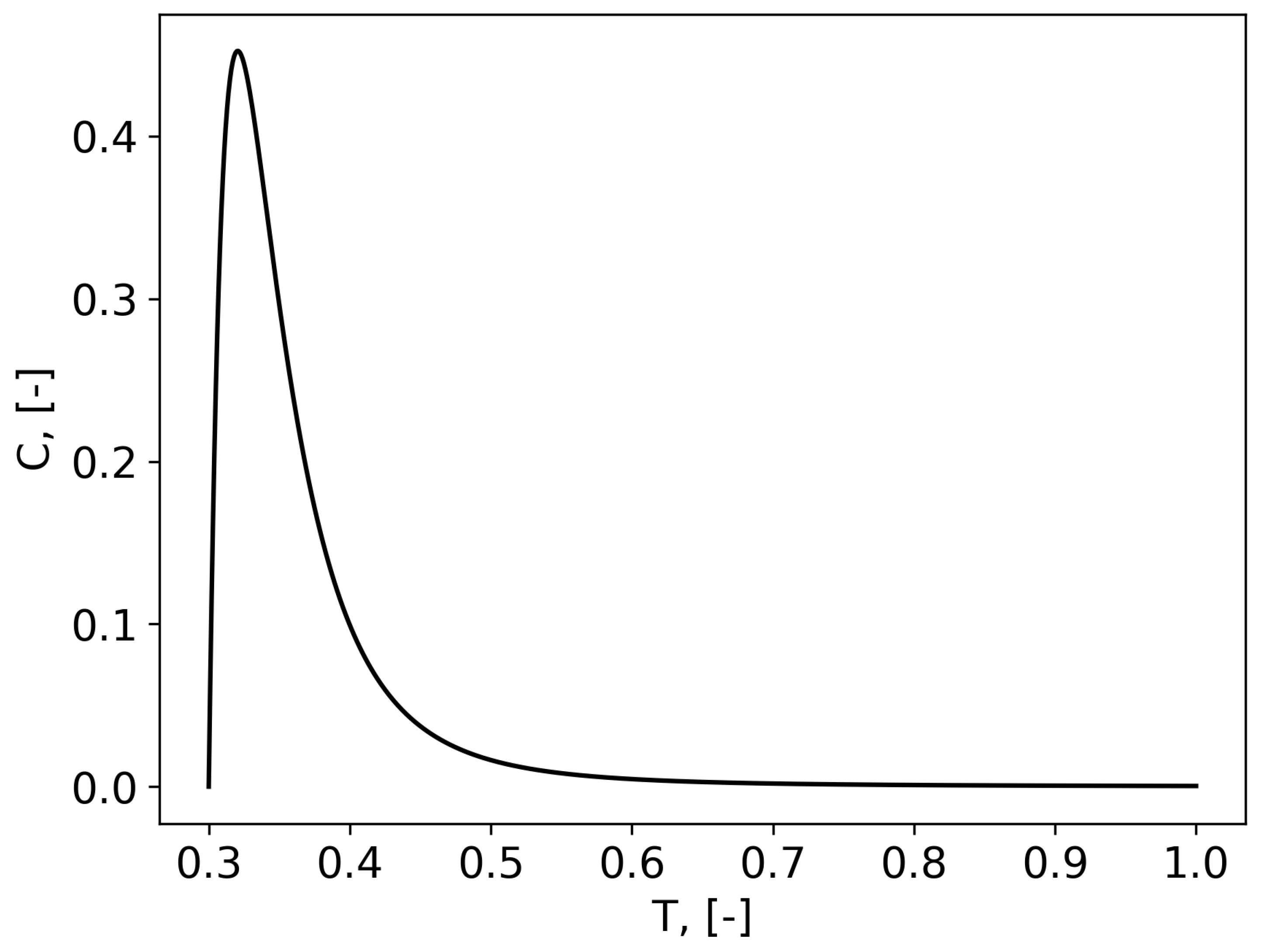
Note that $Pe>0$, $Le>0$, $1>\sigma >0$, $N>0$. So $\mathcal{Z}>0$ always. This is a purely convex curve (see Figure 2) with a single peak—a maximum—and is thus of $\Lambda$ type.

This allows us to conclude that the system of Equations (9)–(12) is of type $K\Omega -\Lambda$. We will utilize this classification in Section 3.

2.5. Critical Conditions for the Onset of Unconventional Propagation

Using the formulation in Section 2.2, we can estimate the critical $Pe$ values for unconventional propagation, which is characterized here by the emergence of solitonary structures. These criteria are defined in [25] (eq. 9.17),

$$k_{\theta }^{\prime }<-\left[L{e}^2{K}_{\eta }^{\prime }+2Le{\left(K_{\eta }^{\prime }{k}_{\theta }^{\prime }-K_{\theta }^{\prime }{k}_{\eta }^{\prime }\right)}^{1/2}\right].$$

(16)

Substituting in (16), Equations (11) and (12) and operating, we obtain a quadratic dependence for the critical value,

$$aP{e}_c^2+bP{e}_c+c=0,$$

(17)

with

$$\begin{array}{cc}\hfill & a=\left(C{N}^3{\Sigma }^{3}exp\left[N(1-T^{-1})\right]\right)/\left(2Le{T}^2\right),\hfill \end{array}$$

(18)

$$\begin{array}{cc}\hfill & b=-N\Sigma \sqrt{2\pi exp\left[N(1-T^{-1})\right]},\hfill \end{array}$$

(19)

$$\begin{array}{cc}\hfill & c=-N^2{\Sigma }^{2}exp\left[N(1-T^{-1})\right],\hfill \end{array}$$

(20)

and $\Sigma =1-\sigma$. Only the positive root has physical sense. Particularization of the approximate Formula (16) with typical values, $\sigma \approx 1/3$, $N\approx 5$, $Le\approx 1/3$, delivers $P{e}_c\approx 21$. This can be compared with the value $Pe=15$ extracted statistically from experiments in [4].

This represents a surprisingly small discrepancy, especially considering the simplifications made during the derivation of the formula. Notable among these approximations are: (a) Usage of a reaction-diffusion model, which disregards product expansion and decouples combustion from the velocity field. (b) The heat-loss model, which is derived from a simplified 1D assessment. (c) The omission of realistic 3D boundary conditions—even if a 2D treatment were feasible—which means significant transversal effects, such as those from the boundary layer, are ignored. (d) The estimation of chemical parameters (such as activation energy) for an equivalent single-step reaction system, which remains a controversial topic in its own right. Significantly, this last point also affects the statistical assessment of $P{e}_c$ previously carried out by several of the co-authors. Note that this limitations are also shared by our theoretical analysis of [24].

3. Phenomena Associated

3.1. General

In the previous section, we endeavored a succinct manipulation of the equations of our previous theoretical paper [24] to match our formulation and the one of Kerner and Osipov [25]. The objective was merely to identify the regime of the problem, in order to be able to classify it.

The theory of autosolitons [25], identifies several phenomena as typical of the $K\Omega -\Lambda$ category. Those are: (a) feature of traveling isolated solutions; (b) propensity to breaking and splitting; (c) existence of periodic results; (d) proclivity to pulsating structures.

Among the phenomena related to periodic solutions, the theory clearly distinguishes several phenomena that can be related to our experiments. Namely, splitting on hot locations and the period doubling—also called re-pumping (the interaction of periodic solutions to alter wavelengths). For pulsating solutions, two singular configurations are described that are of specific interest for us: in particular the rocking and winding behaviors.

Kerner & Osipov [25] provide mathematical expressions to quantify the listed regimes, significantly their ranges of existence, as a function of the bifurcation parameter. Nevertheless, the expressions available in [25] circumscribe themselves to 1D problems. A more adequate dedicated 2D-approach can be found in Liehr [9], summarizing results also obtained with Moskalenko e.g., [38]. Notably these authors managed to obtain a partial differential equation to describe the dynamics of each structure, alone or interacting with other waves. Still, this theory is not applicable to our system. To this one has to add the very limited algebraic description of the 2D-finger flames. All together, these difficulties prevent us, on the short term, to give a concrete mathematical expression for the ranges of existence of each of the regimes. In light of these conditions, we can still inspect the experiments and provide evidence of the existence of some previously mentioned phenomena.

In what follows we will present numerous photographs extracted from the experimental matrix reported in [5,23,37]. Shortly summarizing, the pictures were taken utilizing a Hele-Shaw cell positioned vertically. The narrow thin gap created between the two parallel plates was filled with premixed hydrogen-air with different compositions at normal conditions. Three of the sides of the slit were closed. In the fourth the ignition equipment was positioned. In the photographs, fresh mixtures are represented in light grey tones. The much darker thin traces are caused by the presence of steam. To be able to identify the particular conditions of the realization, in each plot the captions of the figures indicate the experiment number, the rescaled amount of heat loss, $\nu$, the composition of the mixture in terms of % H₂ and the thickness of gaseous slit between the plates.

3.2. Traveling Autosoliton

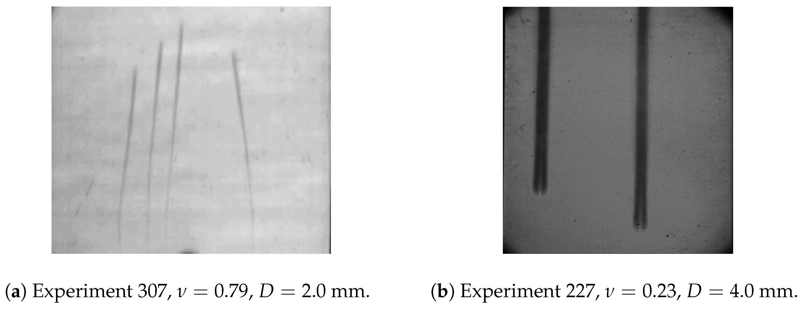
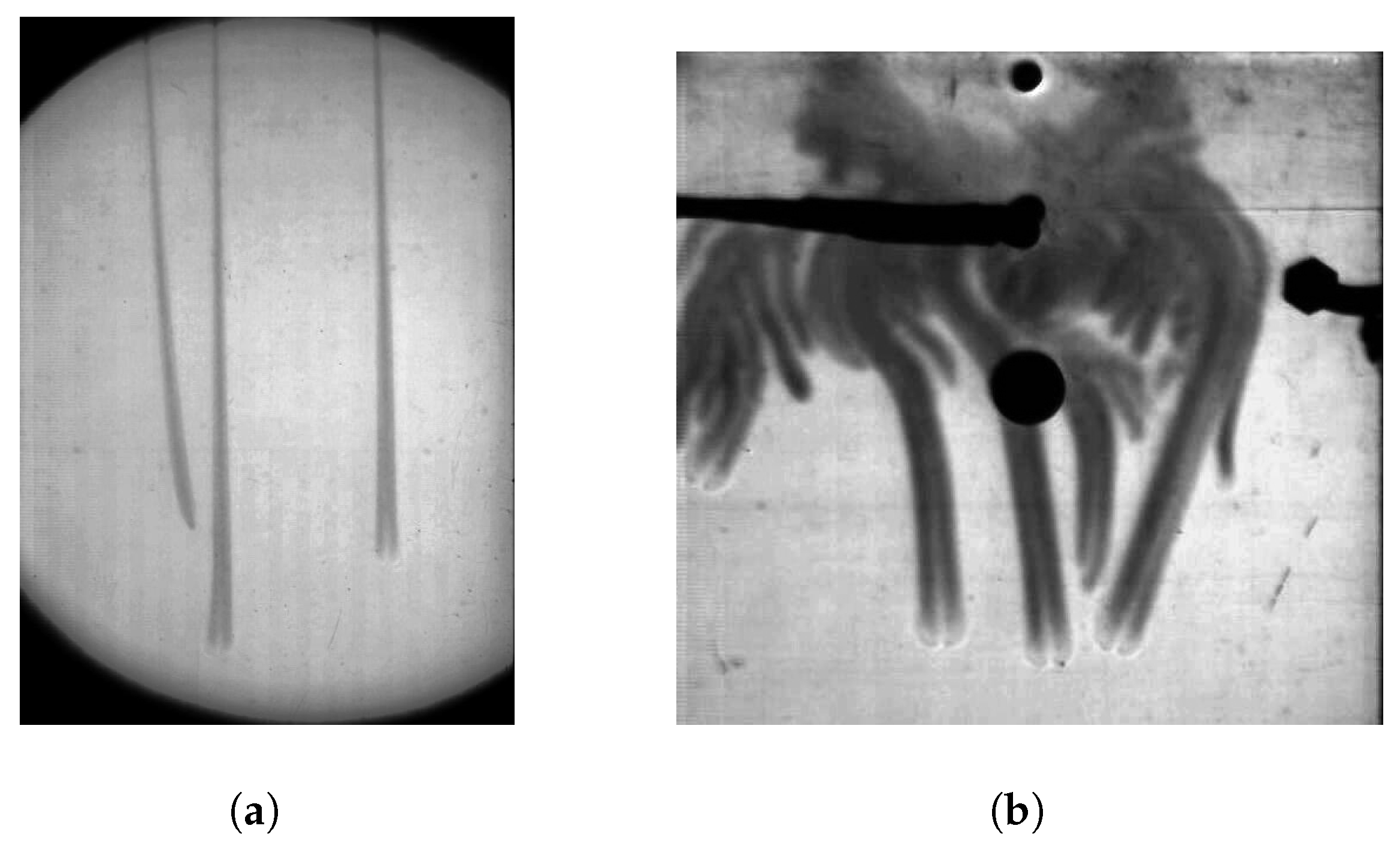
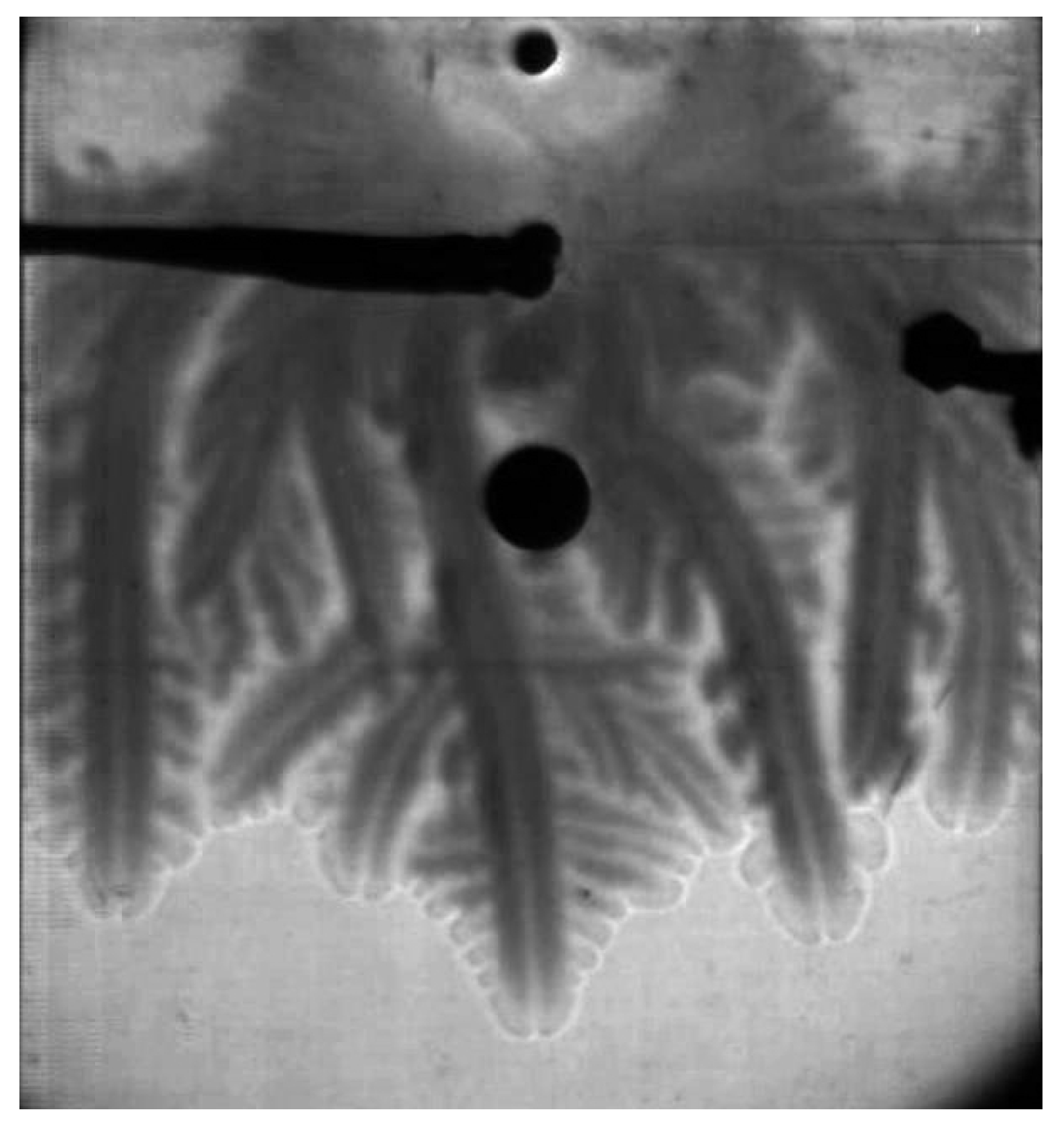
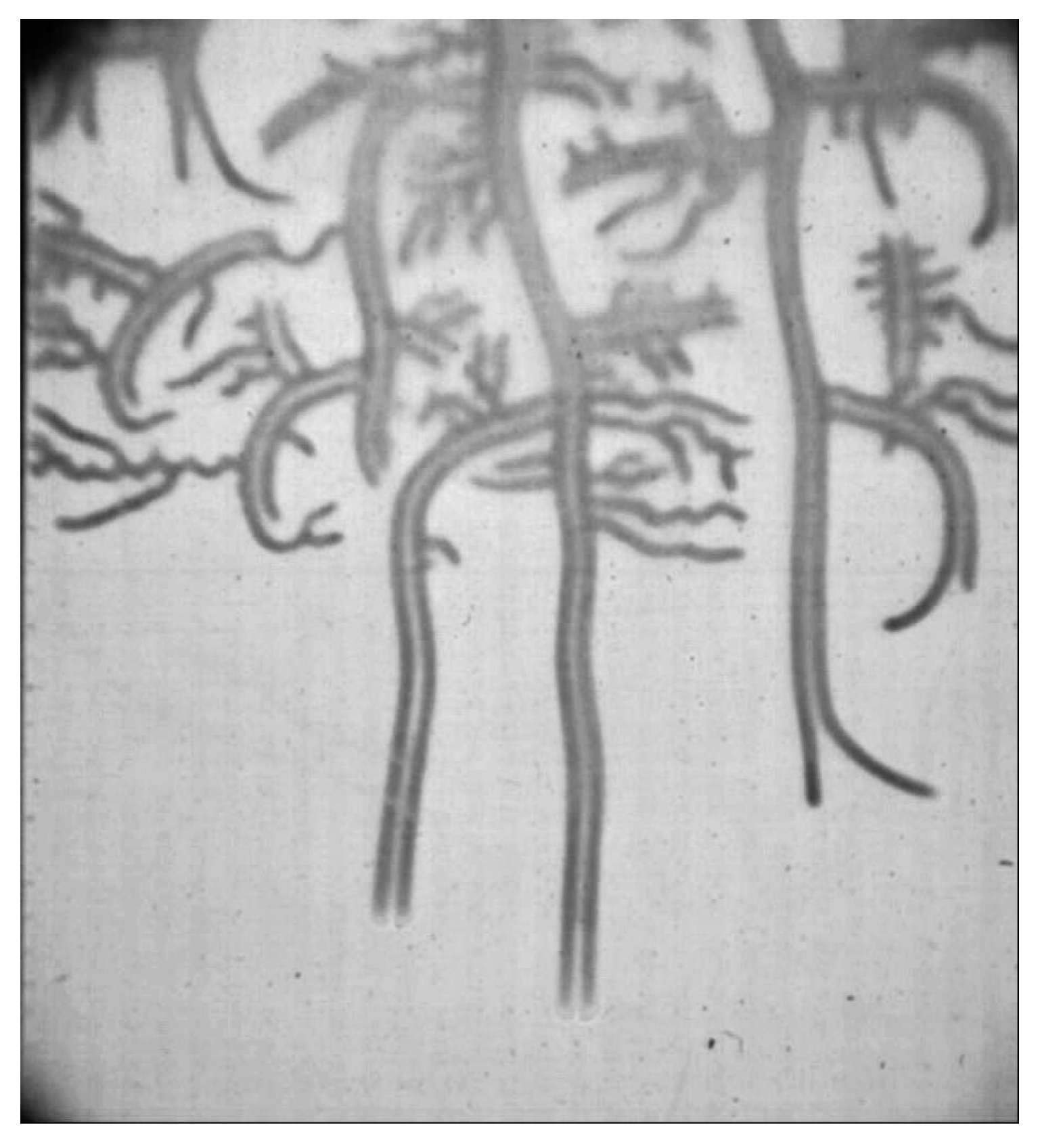
The most simple configuration that the soliton adopts is the steady traveling solution, Figure 3. Note that this steady propagation regime exists both with single-headed (Figure 3a left group travel in parallel trajectories) and two-headed fingers (Figure 3b).

To these conditions, specially the one of Figure 3a, apply the analysis of [20,24,39], where propagation velocity and size of the structures was theoretically deduced. For an additional insight we address the readers to these references.

3.3. Pulsating Autosolitons

Existence of pulsating autosolitons is related to the stability of the steady solution. In the stability problem described in [25] (Chapter 12) it is concluded that only two perturbations are relevant for the stability problem. Those correspond to symmetric and anti symmetric modes that induce solutions as the one represented in Figure 4a and Figure 5a.

3.3.1. Winding

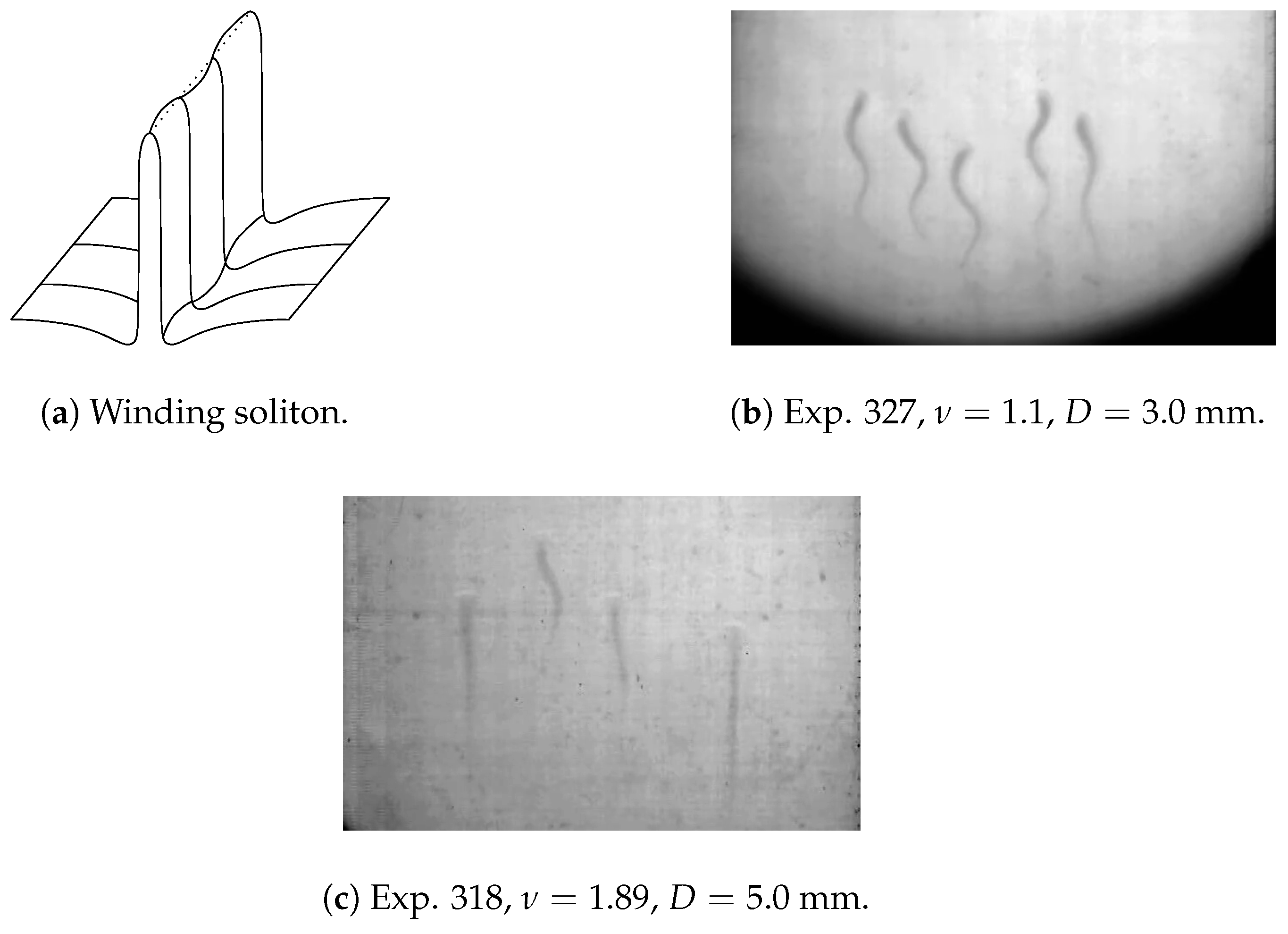
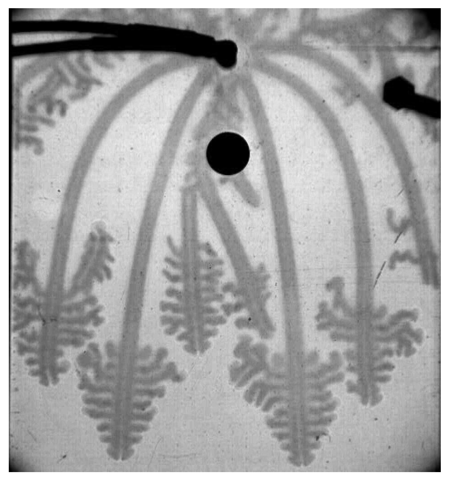
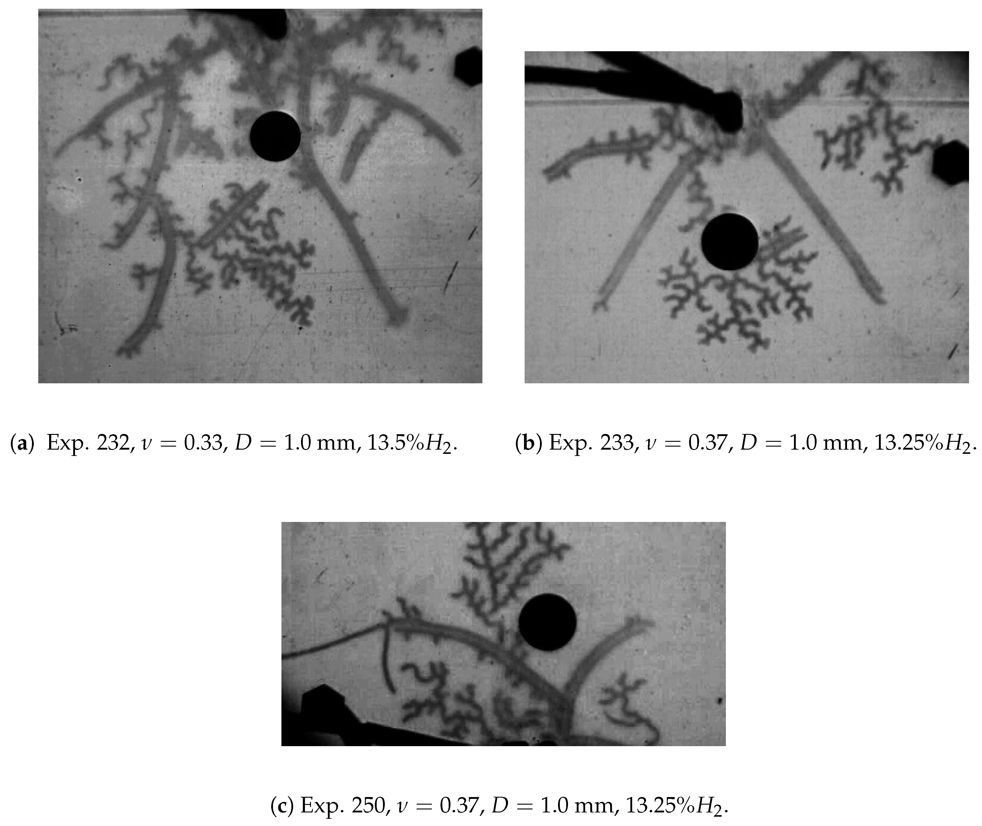
The winding unstable solutions have been detected in several experiments, Figure 4. In order to follow a reasonable narrative, at this stage we exclude splitting and periodic experiments (Section 3.4, Section 3.5 and Section 3.5.2). The experiments shown in Figure 4b,c exhibit this winding behavior. Note that the Figure 4c shows the coexistence of winding (inner) and steady regimes (outer fingers). Also, one should remark that the period and amplitude of oscillation of the two inner fingers are not the same. The propagation velocity of all structures is nevertheless equal.

3.3.2. Rocking

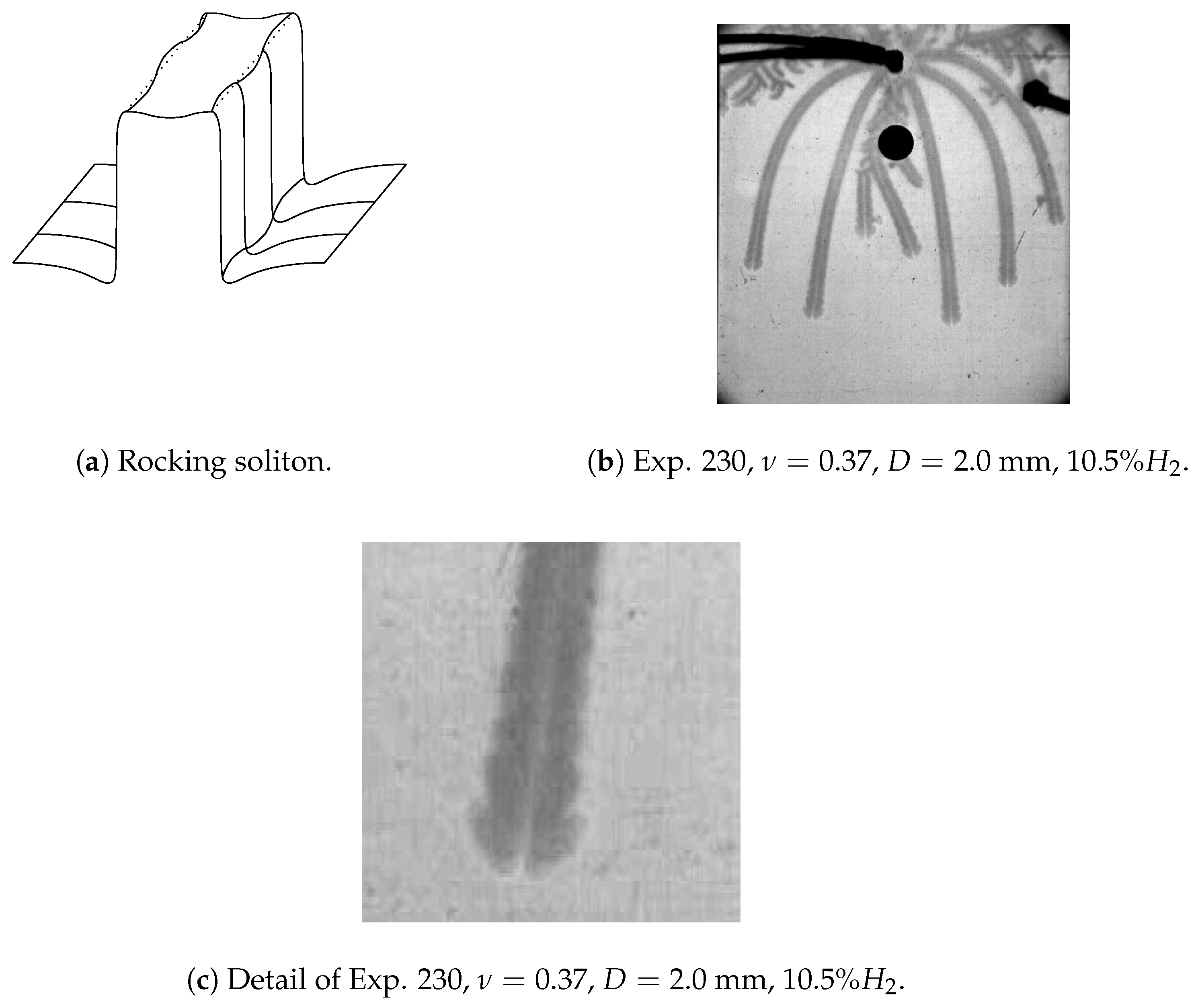
The second unstable configuration is generated by a symmetric mode, relative to the center of the soliton, Figure 5. The profile of the soliton oscillates like in Figure 5a, changing the width of the structure. Such changes can be seen in the shadowgraphy of Figure 5b. The uneven density and steam traces, can also be seen in detail, for a single finger in Figure 5c.

3.4. Splitting

In Figure 5c one sees that the pulsations of the rocking soliton are not steady but grow in amplitude. In mathematical terms, this may be connected with one of the possible mechanisms of splitting. In it, the range of existence of the soliton is exceeded, in terms of width, during one of the oscillations. Typically, the mechanism of this unstable breathing regime may be associated with a main eigenvector with a small but positive real part—non-steadiness—complemented by the next two eigenvectors of non-zero imaginary part, which signify a secondary Hopf bifurcation [40].

Excluding periodic phenomena, breaking of the soliton may occur at its center or in its periphery:

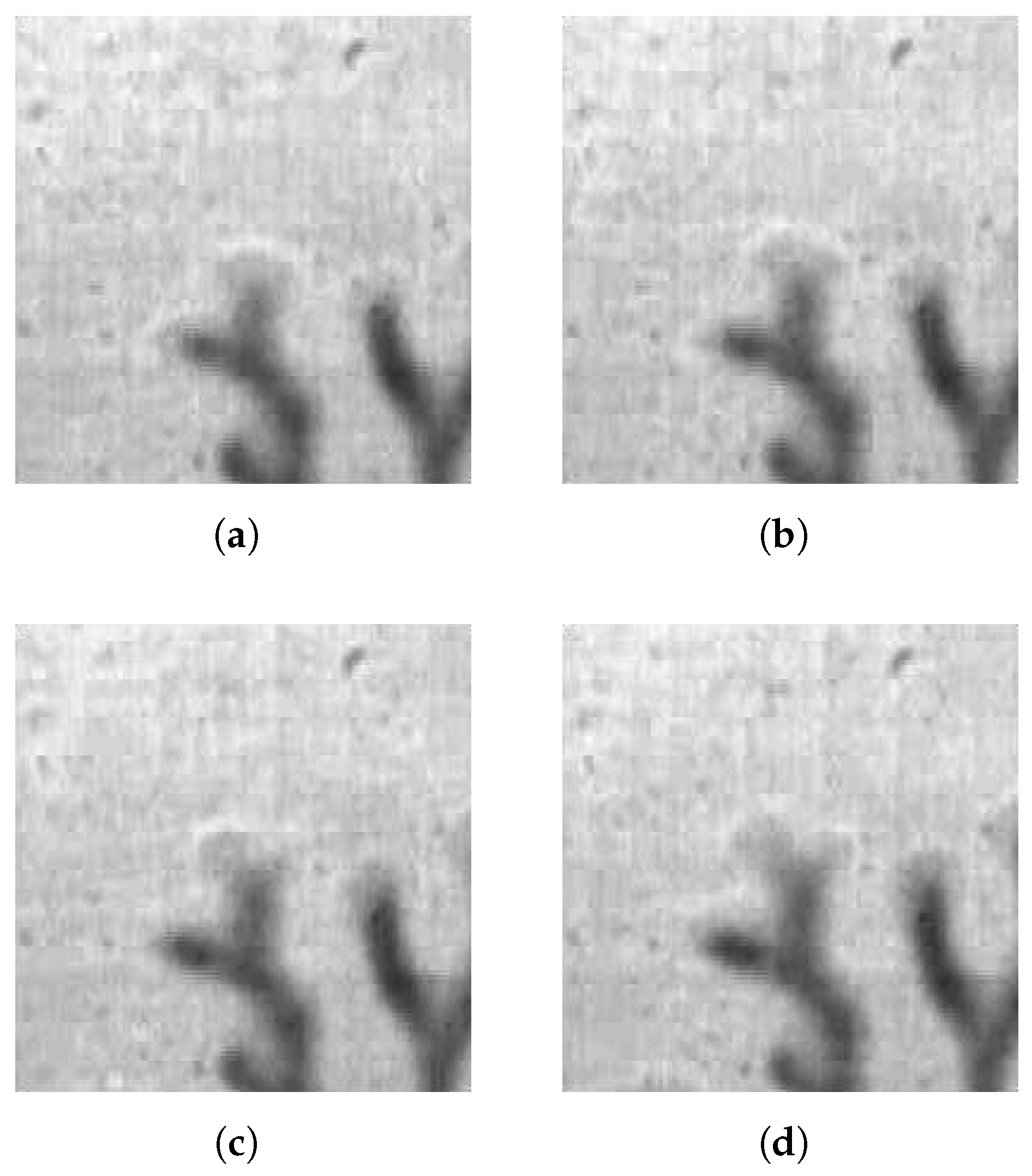
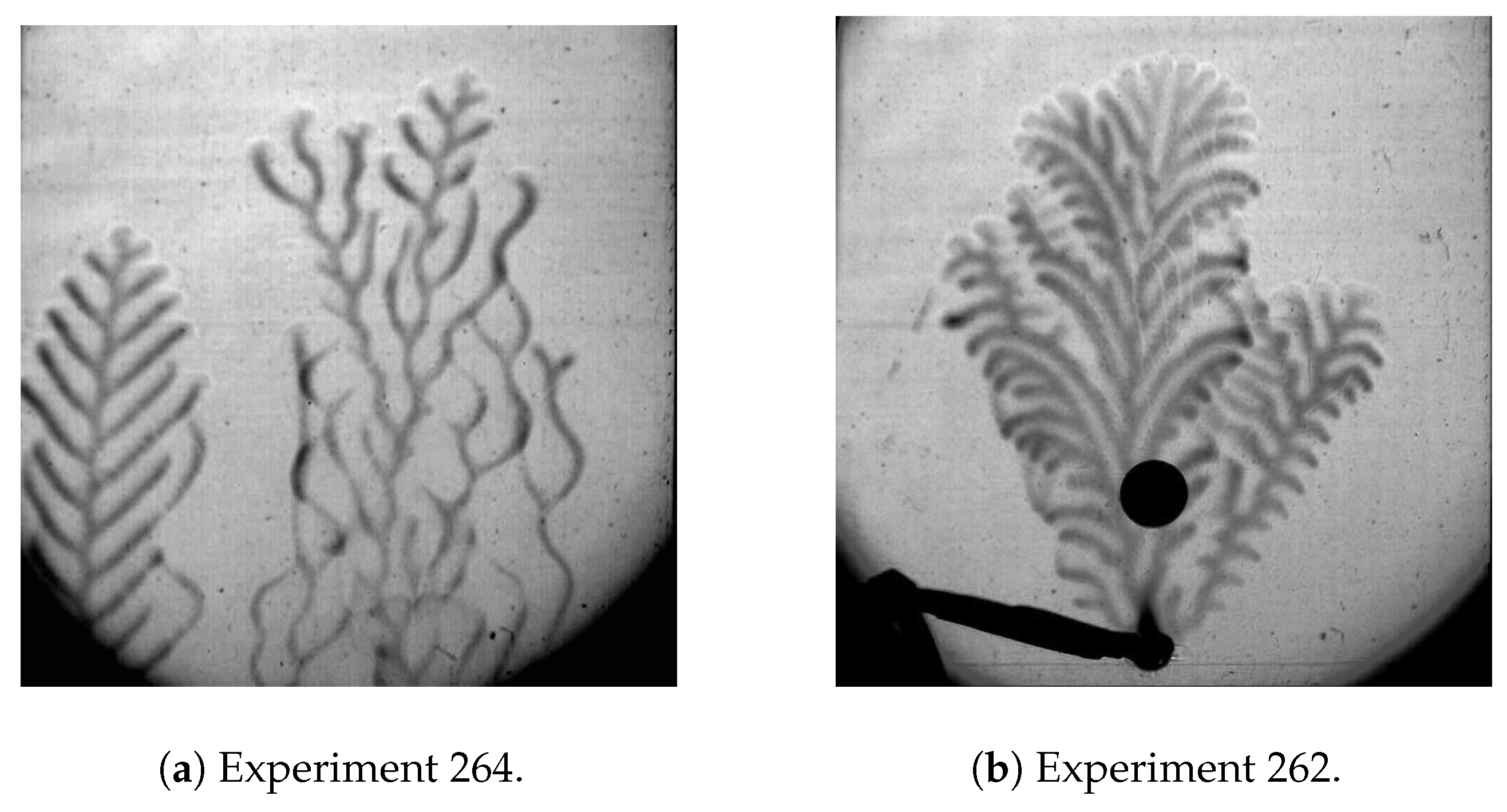
• The splitting in the center, is attributed to the exhaustion of the fuel [25] (Chapter 11). This is seen in Figure 6, and it is by far the most common mechanism we have observed in the experiments;
• The splitting in the periphery appears to be connected with a local decrease of the temperature, that in turn produce a local extinction [25] (Chapter 20.1.2). This process is shown in the snapshots of Figure 7.

Figure 6. (a–d) Splitting in the center. Successive flamelets every 133 ms. Experiment 264, $\nu =1.21$, $D=4.0$ mm, $\%H_2=6.5$.

Figure 6. (a–d) Splitting in the center. Successive flamelets every 133 ms. Experiment 264, $\nu =1.21$, $D=4.0$ mm, $\%H_2=6.5$.

Figure 7. (a–e) Splitting in the periphery. Successive flamelets every 133 ms. Experiment 230, $\nu =0.37$, $D=2.0$ mm, $\%H_2=10.5$.

Figure 7. (a–e) Splitting in the periphery. Successive flamelets every 133 ms. Experiment 230, $\nu =0.37$, $D=2.0$ mm, $\%H_2=10.5$.

Note that these two mechanisms, universally formulated for any kind of solitons, appear to be in agreement with the topologies appearing in [13,14].

Also, one should see that this two ways of splitting determine the general topology of the flame that is finally observed: (a) Peripheral splitting results in cluster (or bunch) shapes, Figure 8; (b) Splitting in the center produces anemone (or fern) like patters, Figure 9.

3.5. Periodic Solutions

Periodic autosolitons are analogous to isolated ones. The most significant difference lies on the conditions in the middle of the space among strata [25] (Chapter 14). Values for temperature and concentration are different to the ones applying for isolated solutions. Namely, a higher temperature and some product concentration should be found in this location. The main characteristics of periodic solutions are reported to be: (a) the period; (b) The thickness of the strata. Both are functions of the bifurcation parameter, and thus proportional to $Pe$ number.

3.5.1. Non Uniqueness of the Solution

Autosolitons with different periods are known to exist simultaneously in the same conditions. This can be also confirmed for our system, see Figure 9. Note that in the experiment shown in Figure 9a two distinct periods were achieved. In the same conditions, a third solution of much smaller period existed, Figure 9b. In all these experiments the ignition was equal. Note that in the later case (Figure 9b), even the two heads structure, in form of parallel propagating strata appeared.

Figure 9. Anemone (or fern) like patterns & Non uniqueness of the solution. Experiments at $\nu =1.21$, $D=4.0$ mm, $6.5\%H_2$.

Figure 9. Anemone (or fern) like patterns & Non uniqueness of the solution. Experiments at $\nu =1.21$, $D=4.0$ mm, $6.5\%H_2$.

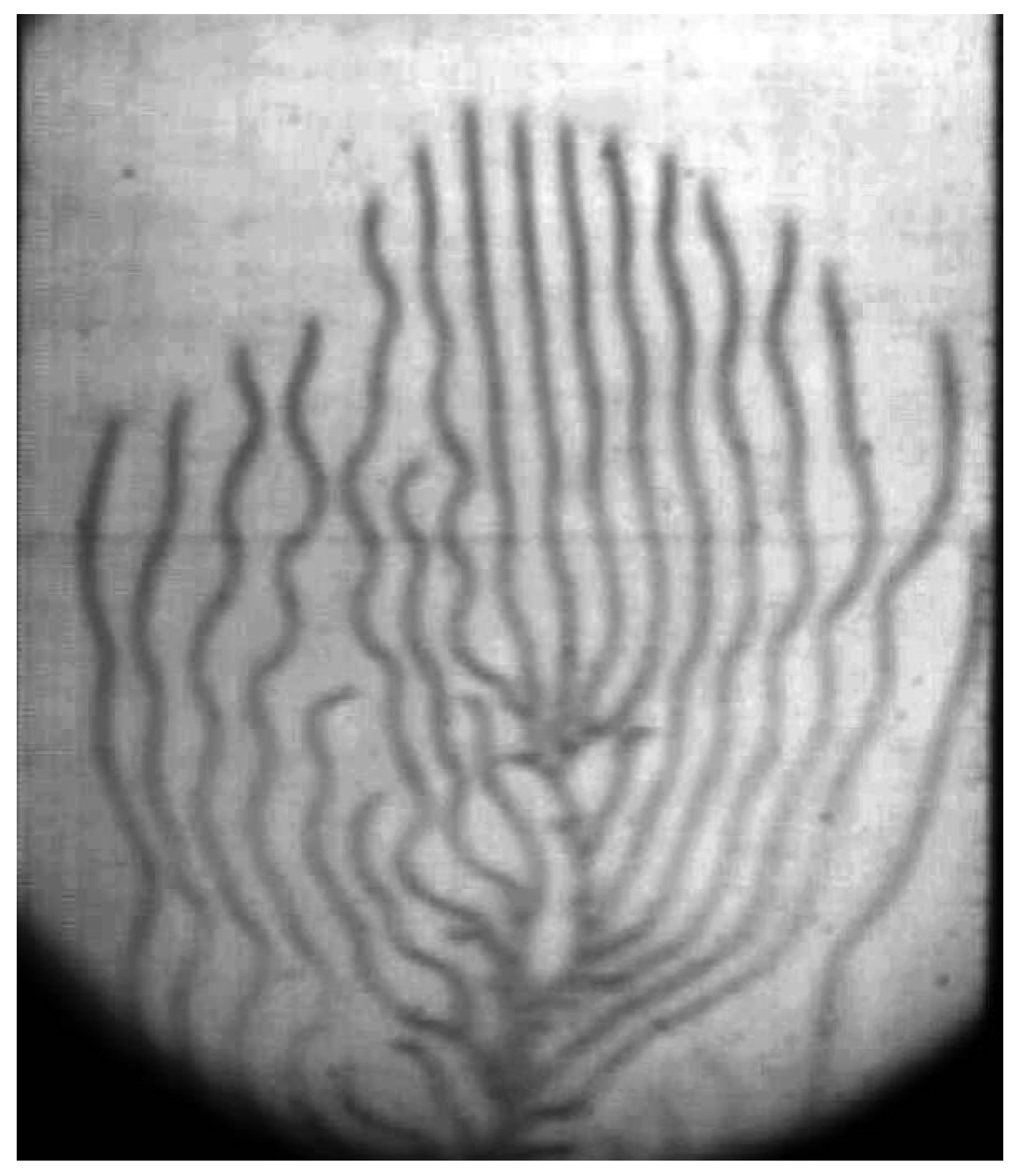
The multiplicity of regimes reported above does not circumscribe itself to the period of the solitons. It also affects the stability of the propagation regime in terms of pulsations. In Figure 9a, the left branch show a stable propagation, whilst the right one has a very pronounced winding. Mixing of stable and unstable regimes can also happen in the same branch. In spite of the quite uniform period, we see stable and winding propagation in different areas of Figure 10.

3.5.2. Splitting and Period Doubling

The splitting of individual solitons has been addressed in Section 3.4. But there are additional reasons causing the branching of the structures. Splitting can also be due to periodic phenomena. This happens when the intervals among the hot strata of the solitons exceed—above or below—the range for which the solutions are stable. It is reported [25] that stability can be regained through two phenomena: (a) Splitting at the center of the structure; (b) Period doubling.

Splitting at the center of the hot strata (Figure 6) diminish the distance among the flamelets. Thus, it may bring the interval among structures again into the stable range. Examples at which this phenomenon is present can also be found in Figure 9a and Figure 10.

On the contrary, in period doubling the amplitude among solitons increases by suppression of adjacent structure or structures. Period doubling promotes fuel diffusion, decrease the importance of diffusion of products, and tends to increase the temperature in the remaining active solitons. Period doubling can be collective -involving several solitons that simultaneously disappear- or localized. In systems with significant inhomogeneities, a local breakdown of the stratum involving the suppression of a single neighboring structure is the normal behavior, see Figure 11.

As shown in Figure 11a, the leftmost flamelets do not propagate parallel to one another; instead, they follow oblique, intersecting trajectories. This contrasts sharply with the images in Figure 3. For instance, Figure 3a displays a group of entirely parallel and steady structures on the left. This behavior is also observed in Figure 3b, as well as in Figure 4b,c, despite the winding of the structures in the latter two pictures. Finally, note the small, single-headed feature in Figure 11b arising from the rightmost double-headed structure, which is beginning to grow in the same direction as the two leftmost branches.

In our opinion, period doubling also occurs in Figure 10. Here, the fifth and sixth branches—from left to right—disappear, annihilated by nearby structures. After their extinction, the fourth and seventh branches oscillate very significantly, suggesting a transitional period. We may compare the winding of these fourth and seventh branches with the steady stable propagation of the tenth to fourteenth ones. We note that the period between the former is noticeably larger than among the latter.

3.5.3. Short Period Solutions

As mentioned before, one of the main differences between periodic and isolated solutions lies in the boundary between two flamelets. In the event of relatively large periods, such as the ones of Figure 5b, interaction between neighbor strata is weak. Thus, conditions between the solitons are close to the values at infinite. Conversely, for experiments in which small periods are registered, one should expect severe change in the state of reagents between adjacent structures.

At this stage, we wish to show that short period, but clearly isolated solutions are possible. Concretely, we want to show the existence of: (a) mono-cellular solutions with relatively high strata thickness and low period (that is, period very close to hot strata thickness), Figure 12; (b) bi-cellular-mono-cellular solutions with low period Figure 13.

Note that the regimes described above, in which the period is similar to the width of the hot strata, can also be interpreted conventionally as periodic cold autosolitons [25]. In the latter the singularity is no longer constituted by the hot strata, but by the cold one.

3.5.4. Zig-Zag Patterns

In this section, we make a small digression to discuss a regime found exclusively in numerical experiments until now. Diagonal or transverse patterns were found numerically by Dejoan et al. [41]. In the calculations of these authors, a structure of diagonal propagation appears as a periodic regime for 2D-flame balls. Notably, the authors studied the period among the structures and found it dependent on the heat losses.

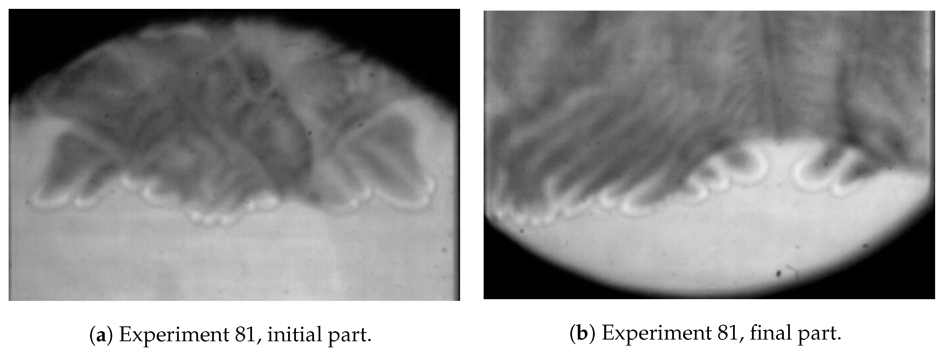
In our Hele-Shaw experiments, we have detected a similar pattern; see Figure 14. In our case, it was found only for reduced heat losses, $\nu \approx 0.08$ corresponding to a $Pe\approx 25$. Those values clearly lie over the threshold of front decomposition. So, in this experiment, we cannot speak properly of flameballs but more concretely about an intermediate regime in which anomalies are starting to appear in the front structure. Therefore, the regime should be treated as a transitional additional pattern, and consequently, it is not included in the core 2D flameball classification. In spite of this, we believe it is important to include this pattern, and believe that the comparison with Dejoan’s results fully justifies its incorporation. By this we try to confirm experimentally, at least partially, the existence of such regime.

In our experiment, the reduced heat losses have translated into a very short period among structures. Still the diagonal pattern is clearly visible in Figure 14. The sense of the propagation is not uniform in the whole domain. This results into the characteristic zig-zag pattern observable in Figure 14. That zig-zag is also partially visible in the numerical results of [41].

3.5.5. Bi-Cellular Flamelet

Among the short period solutions, probably the most notable structure is the bi-cellular structure itself. Note that this structure appears quasi isolated, with flamelets separated by long periods, Figure 3a, Figure 5a and Figure 11a, isolated but separated with short periods, Figure 11b, or in conjunction with mono-cellular fingers, Figure 8 and Figure 13.

It may be appropriate to discuss now, in view of the periodic treatment of the solutions of the sections above, whether the by-cellular configuration is a structure in its own or it is simply constituted by two flamelets closely assembled together. The former constitutes the original interpretation [4,5,23]. We will discuss here the latter, inspired by the theory of [9,25].

The experiments of Figure 3b, Figure 5b and Figure 11b suggest that the range of stable periodic solutions (as function of the bifurcation parameter) is segmented in two distinct regions. In the respective conditions of these experiments we see some short wavelength area in which the bi-cellular structure lies, separated from a long wavelength domain applying to the periods among different fingers.

Such behavior—two distinct areas of stability with disparate periods separated by an unstable domain, and thus with non-observable wavelengths—has been reported previously for other physical phenomena, notably in 2D and 3D systems [25].

Also in support of the second interpretation we may observe the results contained in Figure 15. In the upper left and lower right corners of the picture, the bi-cellular structure simply splits. After the branching, the trajectories of each of the two cells that had formed the construct are no longer parallel. Additionally, in the middle left part of the illustration, one observes that two bi-cellular fingers suffer partial extinction of only one of the two components.

Partial extinction of one of the two cellular structures can be also seen in Figure 16a–c. In the first two pictures, this extinction is shortly followed by quenching of the other cell. Such behavior has also been detected in numerical calculations, see Figure 10c in [41]. Nevertheless, in Figure 16c (left side), we see the other constituent survives and even escapes the visible area of the experiment.

A theoretical description of a regime constituted by two solitons exists in the literature. This constitutes the so called Bound State [9]. In it, the interaction between the structures is described by a pair of attracting-repulsion forces. In the Bound State these forces find a stable and constant status. The propagation is perpendicular to their interaction direction [42,43,44].

4. Conclusions

In this paper we have reinterpreted the experiments of Veiga et al. [5] through the framework of Synergetics. The latter interdisciplinary knowledge deals with the formation and self-organization of physical systems. For this study we focused concretely on the findings already available for the theory of Solitons.

Building on our previous demonstration that we may utilize a reaction-diffusion system to describe 2D-flamelets [20], we have translated the original formulation into the formalism applying to soliton theory. Note that both are very similar, but the latter has allowed us to classify our system in terms of the theory of solitary waves. Then, we have identified the propagation patterns described in the monographs devoted to the Soliton theory applying to our regime. Finally, we have studied the propagation appearing in the experiments identifying some of the patters described in the theory.

This allowed us to conclude that the classification previously adopted was largely insufficient. Therefore, we have addressed the reclassification of the experimental results. We found the following typologies:

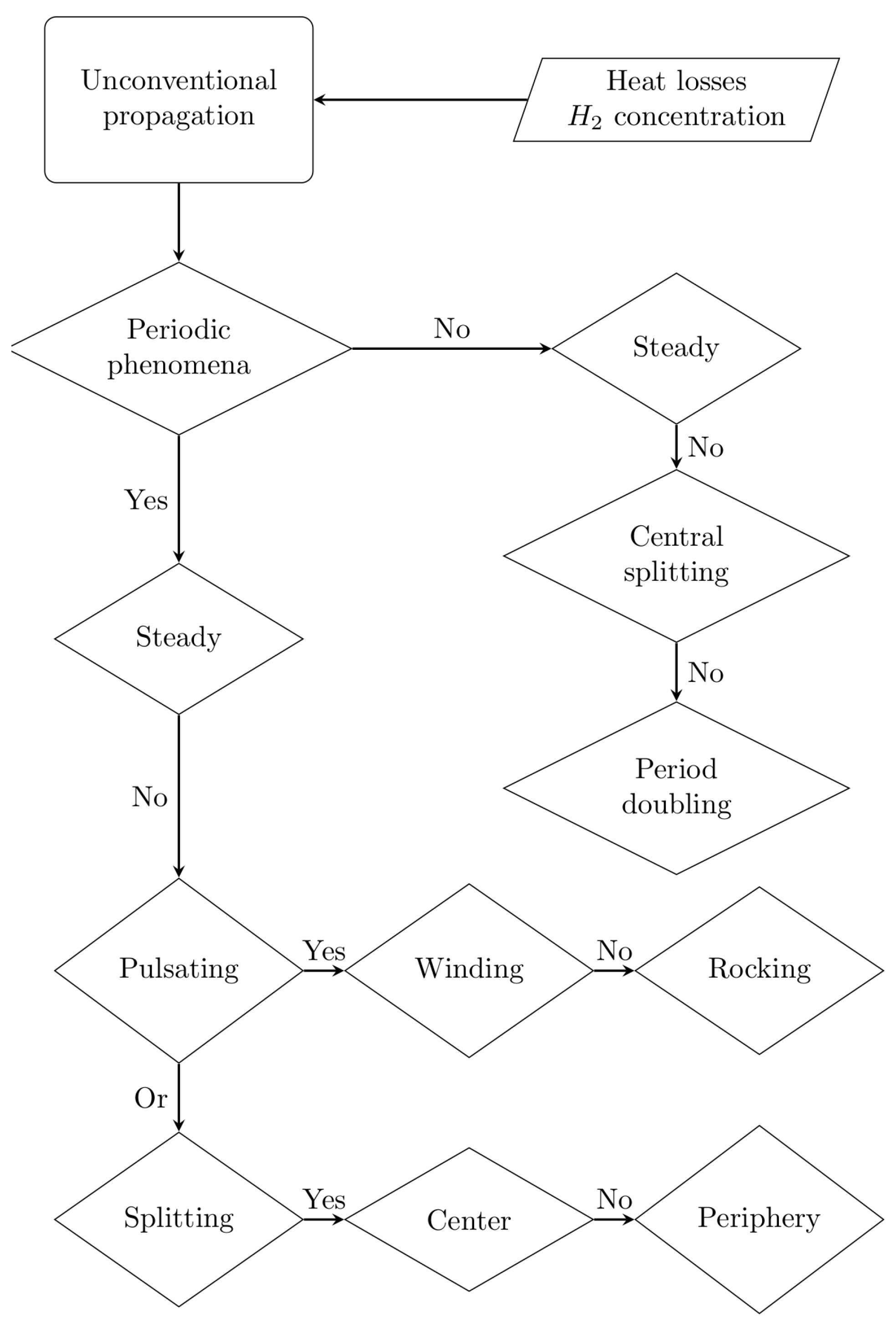
Regarding a single flamelet, propagation can be steady or unsteady. Unsteady regimes encompass pulsating and splitting flameballs. Pulsating can occur in two ways, winding and rocking. Splitting can happen in the center of the hot strata or in its periphery.

Periodic solutions can have multiple wavelengths simultaneously. Individual members of the ensemble can pulsate or not. Periodic solution can interact with each other, increasing or decreasing its period (period doubling and re-pumping).

Because the previous categorizations are complex, we have tried to clarify the multiple typologies detected by Figure 17.

References

1. Kuznetsov, M.; Grune, J. Experiments on combustion regimes for hydrogen/air mixtures in a thin layer geometry. Int. J. Hydrogen Energy 2019, 44, 8727–8742. [Google Scholar] [CrossRef] [Scilit]
2. Schlichting, H. Grenzschichttheorie; Braun, G., Ed.: Karlsruhe, Germany, 1951; p. 326. [Google Scholar]
3. Veiga-López, F.; Martínez-Ruiz, D.; Kuznetsov, M.; Sánchez-Sanz, M. Thermoacoustic analysis of lean premixed hydrogen flames in narrow vertical channels. Fuel 2020, 278, 118212. [Google Scholar] [CrossRef] [Scilit]
4. Escanciano, J.Y.; Kuznetsov, M.; Veiga-López, F. Characterization of unconventional hydrogen flame propagation in narrow gaps. Phys. Rev. E 2021, 103, 033101. [Google Scholar] [CrossRef] [Scilit]
5. Veiga-López, F.; Kuznetsov, M.; Martínez-Ruiz, D.; Fernández-Tarrazo, E.; Grune, J.; Sánchez-Sanz, M. Unexpected propagation of ultra-lean hydrogen flames in narrow gaps. Phys. Rev. Lett. 2020, 124, 174501. [Google Scholar] [CrossRef] [Scilit] [PubMed]
6. Zik, O.; Olami, Z.; Moses, E. Fingering instability in combustion. Phys. Rev. Lett. 1998, 81, 3868. [Google Scholar] [CrossRef] [Scilit]
7. Zik, O.; Moses, E. Fingering instability in combustion: An extended view. Phys. Rev. E 1999, 60, 518. [Google Scholar] [CrossRef] [Scilit]
8. Zhang, Y.; Ronney, P.; Roegner, E.; Greenberg, J. Lewis number effects on flame spreading over thin solid fuels. Combust. Flame 1992, 90, 71–83. [Google Scholar] [CrossRef] [Scilit]
9. Liehr, A. Dissipative Solitons in Reaction Diffusion Systems; Springer: Berlin/Heidelberg, Germany, 2013. [Google Scholar]
10. Kurdyumov, V.N.; Matalon, M. Flame acceleration in long narrow open channels. Proc. Combust. Inst. 2013, 34, 865–872. [Google Scholar] [CrossRef] [Scilit]
11. Kurdyumov, V.N. Propagation of premixed isobaric flames in narrow channels with heat-losses: The asymptotic analysis revised and reliance on the flame-sheet model. Combust. Flame 2019, 206, 138–149. [Google Scholar] [CrossRef] [Scilit]
12. Fernández-Galisteo, D.; Kurdyumov, V.N. Impact of the gravity field on stability of premixed flames propagating between two closely spaced parallel plates. Proc. Combust. Inst. 2019, 37, 1937–1943. [Google Scholar] [CrossRef] [Scilit]
13. Martínez-Ruiz, D.; Veiga-López, F.; Fernández-Galisteo, D.; Kurdyumov, V.N.; Sánchez-Sanz, M. The role of conductive heat losses on the formation of isolated flame cells in Hele-Shaw chambers. Combust. Flame 2019, 209, 187–199. [Google Scholar] [CrossRef] [Scilit]
14. Domínguez-González, A.; Martínez-Ruiz, D.; Sánchez-Sanz, M. Stable circular and double-cell lean hydrogen-air premixed flames in quasi two-dimensional channels. Proc. Combust. Inst. 2023, 39, 1731–1741. [Google Scholar] [CrossRef] [Scilit]
15. Kagan, L.; Sivashinsky, G. Pattern formation in flame spread over thin solid fuels. Combust. Theor. Model. 2008, 12, 269–281. [Google Scholar] [CrossRef] [Scilit]
16. Moskalev, P.V.; Denisenko, V.P.; Kirillov, I.A. Classification and Dynamics of Ultralean Hydrogen–Air Flames in Horizontal Cylindrical Hele–Shaw Cells. J. Exp. Theor. Phys. 2023, 137, 104–113. [Google Scholar] [CrossRef] [Scilit]
17. Haken, H. An Introduction: Nonequilibrium Phase Transitions and Self-Organization in Physics, Chemistry and Biology; Springer: Berlin/Heidelberg, Germany, 2004; pp. 1–387. [Google Scholar]
18. Haken, H. Advanced Synergetics: Instability Hierarchies of Self-Organizing Systems and Devices; Springer Science & Business Media: Berlin/Heidelberg, Germany, 2012. [Google Scholar]
19. Turing, A.M. The chemical basis of morphogenesis. Bull. Math. Biol. 1990, 52, 153–197. [Google Scholar] [CrossRef] [Scilit] [PubMed]
20. Yanez, J.; Kagan, L.; Kuznetsov, M.; Sivashinsky, G. On Disintegrating Lean Hydrogen Flames in Narrow Gaps. Fire 2025, 8, 345. [Google Scholar] [CrossRef] [Scilit]
21. Domínguez-González, A.; Kurdyumov, V.N.; Sánchez, A.L.; Martínez-Ruiz, D. On the existence of propagating circular flames in narrow channels. Combust. Flame 2025, 281, 114415. [Google Scholar] [CrossRef] [Scilit]
22. Mikhailov, A.S. Foundations of Synergetics I: Distributed Active Systems; Springer Science & Business Media: Berlin/Heidelberg, Germany, 2012. [Google Scholar]
23. Veiga López, F. Flame Propagation in Narrow Channels. Ph.D. Thesis, Universidad Carlos III de Madrid, Madrid, Spain, 2020. [Google Scholar]
24. Yanez, J.; Kagan, L.; Sivashinsky, G.; Kuznetsov, M. Modeling of 2D self-drifting flame-balls in Hele-Shaw cells. Combust. Flame 2023, 258, 113059. [Google Scholar] [CrossRef] [Scilit]
25. Kerner, B.S.; Osipov, V.V. Autosolitons: A New Approach to Problems of Self-Organization and Turbulence; Springer Science & Business Media: Berlin/Heidelberg, Germany, 1994. [Google Scholar]
26. Drazin, P.G.; Johnson, R.S. Solitons: An Introduction; Cambridge University Press: Cambridge, UK, 1989; Volume 2. [Google Scholar]
27. Akhmediev, N.; Ankiewicz, A. Three sources and three component parts of the concept of dissipative solitons. In Dissipative Solitons: From Optics to Biology and Medicine; Springer: Berlin/Heidelberg, Germany, 2008; pp. 1–28. [Google Scholar]
28. Dominguez-Gonzalez, A.; Encinar, M.; Martnez-Ruiz, D. Numerical study on the causality of solution multiplicity in ultra-lean H2-air premixed flames. In 76th Annual Meeting of the APS Division of Fluid Dynamics; American Physical Society: College Park, MD, USA, 2023. [Google Scholar]
29. Zeldovich, Y. Theory of Combustion and Detonation of Gases; Air Matériel Command and Headquarters, Wright-Patterson Air Force Base: Dayton, OH, USA, 1949. [Google Scholar]
30. Ronney, P.D. Understanding combustion processes through microgravity research. Symp. (Int.) Combust. 1998, 27, 2485–2506. [Google Scholar] [CrossRef] [Scilit]
31. Ronney, P.D.; Wu, M.S.; Pearlman, H.G.; Weiland, K.J. Experimental study of flame balls in space: Preliminary results from STS-83. AIAA J. 1998, 36, 1361–1368. [Google Scholar] [CrossRef] [Scilit]
32. Zabusky, N.J.; Kruskal, M.D. Interaction of “solitons” in a collisionless plasma and the recurrence of initial states. Phys. Rev. Lett. 1965, 15, 240. [Google Scholar] [CrossRef] [Scilit]
33. Brailovsky, I.; Sivashinsky, G. On stationary and travelling flame balls. Combust. Flame 1997, 110, 524–529. [Google Scholar] [CrossRef] [Scilit]
34. Minaev, S.S.; Kagan, L.; Sivashinsky, G. Self-propagation of a diffuse combustion spot in premixed gases. Combust. Explos. Shock Waves 2002, 38, 9–18. [Google Scholar] [CrossRef] [Scilit]
35. Sivashinsky, G.I. Some developments in premixed combustion modeling. Proc. Combust. Inst. 2002, 29, 1737–1761. [Google Scholar] [CrossRef] [Scilit]
36. Matkowsky, B.; Sivashinsky, G. An asymptotic derivation of two models in flame theory associated with the constant density approximation. SIAM J. Appl. Math. 1979, 37, 686–699. [Google Scholar] [CrossRef] [Scilit]
37. Kuznetsov, M.; Yanez, J.; Veiga-López, F. Near Limit Flame Propagation in a Thin Layer Geometry at Low Peclet Numbers. In Proceedings of the 18th International Conference on Flow Dynamics (ICFD 2021), Virtually, 27–29 October 2022; pp. 688–692. [Google Scholar]
38. Liehr, A.; Moskalenko, A.; Purwins, H.G. Transition from stationary to rotating bound states of dissipative solitons. In High Performance Computing in Science and Engineering’03; Springer: Berlin/Heidelberg, Germany, 2003; pp. 225–234. [Google Scholar]
39. Yanez, J.; Kuznetsov, M.; Veiga-López, F. On the velocity, size, and temperature of gaseous dendritic flames. Phys. Fluids 2022, 34, 113601. [Google Scholar] [CrossRef] [Scilit]
40. Gurevich, S.; Amiranashvili, S.; Purwins, H.G. Breathing dissipative solitons in three-component reaction-diffusion system. Phys. Rev. E 2006, 74, 066201. [Google Scholar] [CrossRef] [Scilit]
41. Dejoan, A.; Fernández-Galisteo, D.; Kurdyumov, V.N. Numerical Study of the Propagation Patterns of Lean Hydrogen-Air Flames Under Confinement. In Proceedings of the 29th ICDERS, SNU, Siheung, Republic of Korea, 23–28 July 2023. [Google Scholar]
42. Bode, M.; Liehr, A.; Schenk, C.; Purwins, H.G. Interaction of dissipative solitons: Particle-like behaviour of localized structures in a three-component reaction-diffusion system. Phys. D Nonlinear Phenom. 2002, 161, 45–66. [Google Scholar] [CrossRef] [Scilit]
43. Schenk, C.P. Numerische und Analytische Untersuchung Solitärer Strukturen in Zwei-und Dreikomponentigen Reaktions-Diffusions-Systemen. Ph.D. Thesis, Westfälische Wilhelms-Universität Münster, Münster, Germany, 1999. [Google Scholar]
44. Moskalenko, A. Dynamische Gebundene Zustände und Drift-Rotations-Dynamics von Dissipativen Solitonen. Master’s Thesis, Westfälische Wilhelms-Universität Münster, Münster, Germany, 2002. [Google Scholar]
Figure 1. Unconventional flame propagation categories: (a) one-headed finger, (b) one-headed branching, (c) two-headed fingers, and (d) two-headed branching. Reprinted with permission from Yanez Escanciano et al., Phys. Rev. E 103, 033101, 2021 [4]. Copyright (2021) by the American Physical Society.
Fire 09 00288 g001
Figure 2. Typical shape of of the null-cline curve.
Fire 09 00288 g002
Figure 3. Steady traveling solutions.
Fire 09 00288 g003
Figure 4. Winding traveling solutions.
Fire 09 00288 g004
Figure 5. Rocking traveling solutions.
Fire 09 00288 g005
Figure 8. Cluster (or bunch) shape. Experiment 230, ν = 0.37 , D = 2.0 mm, % H 2 = 10.5 .
Fire 09 00288 g008
Figure 10. Mixing of stable and unstable regimes: quasi-steady and winding propagation. Experiment 305, ν = 0.58 , D = 2.0 mm, % H 2 = 9.75 .
Fire 09 00288 g010
Figure 11. Localized period doubling. (a) Experiment 339, ν = 0.41 , D = 3.0 mm, 9.0 % H 2 . (b) Experiment 287, ν = 0.27 , D = 4.0 mm, 8.75 % H 2 .
Fire 09 00288 g011
Figure 12. Low period large thickness solutions. (a) Experiment 300, ν = 0.73 , D = 6.0 mm, 6.0 % H 2 . (b) Experiment 315, ν = 0.77 , D = 5.0 mm, 6.5 % H 2 .
Fire 09 00288 g012
Figure 13. Experiment 285, ν = 0.19 , D = 4.0 mm, % H 2 = 9.25 .
Fire 09 00288 g013
Figure 14. Diagonal patterns: Experiment 81, ν = 0.08 , D = 6.0 mm, % H 2 = 9.5 .
Fire 09 00288 g014
Figure 15. Splitting & Partial extinction of one of the two cellular structures. Experiment 198, ν = 0.37 , D = 2.0 mm, % H 2 = 10.5 .
Fire 09 00288 g015
Figure 16. Mono-celular and bi-cellular finger flames.
Fire 09 00288 g016
Figure 17. Typologies detected.
Fire 09 00288 g017
Disclaimer/Publisher’s Note: The statements, opinions and data contained in all publications are solely those of the individual author(s) and contributor(s) and not of MDPI and/or the editor(s). MDPI and/or the editor(s) disclaim responsibility for any injury to people or property resulting from any ideas, methods, instructions or products referred to in the content.