A Novel Robust HL-Based Transformer Approach for Predicting Electrical Fire Risks

Abstract

Accurate prediction of electrical fire risk is important for early warning, but real-world monitoring data are often affected by sensor noise, transient anomalies, and non-Gaussian interference. This study proposes an HL-Transformer that incorporates an HL-Pooling layer based on the Hodges–Lehmann estimator into the Transformer feature aggregation process. The HL-Pooling layer replaces conventional mean- or max-based pooling by using the median of pairwise averages, aiming to suppress abnormal perturbations while preserving temporal information. Experiments were conducted on a real-world electrical fire monitoring dataset and the public ETTh1 dataset, with additional robustness tests under different outlier ratios and intensities. The results show that, within the same Transformer backbone, HL-Transformer reduced the MSE by 75.4% compared with the Max-Pooling variant and achieved an R² of 0.879 on the electrical fire risk prediction task. Under injected outliers, the HL-Pooling layer showed more stable error trends, and its transfer to TCN, CNN-LSTM, and 1D-CNN models further improved predictive performance. These findings indicate that HL-Pooling is a robust and portable alternative to conventional pooling for time-series forecasting in noisy monitoring environments.

1. Introduction

Electrical fires are characterized by their sudden onset and concealed nature. A wide variety of electrical faults, such as short circuits, circuit overloads, damaged wiring or equipment, and other electrical malfunctions, may trigger them. These faults often generate heat, sparks, or arcs, which may ignite flammable materials surrounding electrical lines or equipment, thereby initiating a fire [1]. According to international fire statistics, electrical distribution and lighting equipment remain an important source of home fire losses, and such fires still cause substantial casualties and property damage [2]. Therefore, accurate early warning for electrical fires is of paramount importance.

With the growing application of Internet of Things (IoT) technologies in fire monitoring, key parameters and alarm signals can be captured through sensor networks to support dynamic state recognition [3]. It is well known that overheating of electrical equipment accounts for approximately 40% of fire incidents. Early warning systems for electrical fires play a crucial role in preventing fires or halting their rapid spread [4,5]. However, traditional detection methods are often highly directional—monitoring specific fire indicators using certain types of sensors [6]. These methods focus narrowly on specific parameters and fail to provide a holistic understanding of fire-related factors and their surrounding environment. In addition, sensor-based fire detection studies show that single-source indicators are easily affected by nuisance signals, and multivariate processing is usually needed to improve sensitivity and false-alarm immunity [7]. Real-time monitoring of electrical cable usage through multiple sensors has become a common fire prevention approach [8]. Nevertheless, it should be noted that real-time data can only reflect current fire risks and lack predictive capability.

To achieve accurate prediction of electrical fire risks, it is essential to first understand the underlying mechanisms of electrical fires and design corresponding analytical methods. Previous studies have shown that electrical fire incidents typically unfold as progressive hazard events, characterized by strong temporal correlations throughout the risk evolution process. The progression—from current overload and line temperature rise to insulation degradation and eventual arc-induced breakdown—reflects a dynamic transition through multiple risk states. While traditional time series forecasting methods are capable of providing early warnings, their performance deteriorates under conditions of increasing system complexity and multi-source interference, often resulting in high false alarm rates. Recent advances in artificial intelligence have brought about a paradigm shift in this domain, with growing attention being paid to deep learning-based models for fire risk prediction [9]. These models can proactively capture fire risk trends and issue timely warnings by mining temporal dependencies within the data.

However, real-world monitoring environments present significant challenges. Data often include anomalies such as transient load spikes, sensor drift, and human operational disturbances, which lead to covariate shifts in the input distributions. Neural networks are particularly sensitive to these distributional changes. Their mechanisms for temporal feature extraction are easily disrupted by outliers, resulting in systematic prediction bias and reduced reliability of the warning system. In this sense, this study primarily addresses the critical challenge of high false alarm rates in time series prediction models used for electrical fire warning systems. The motivation stems from the significant limitations of current deep learning-based early warning systems when operating under complex and dynamic conditions. Conventional neural network architectures tend to be overly sensitive to anomalies in sensor data, which severely restricts their generalization capabilities. In particular, under non-stationary conditions—such as abrupt load fluctuations or transient equipment faults—traditional time series models are especially vulnerable to interference from outliers or extreme values, resulting in fragile statistical behavior and compromised reliability.

To address this technical bottleneck, this study proposes an HL-Transformer model by embedding an HL-Pooling layer based on the Hodges–Lehmann estimator into the Transformer architecture. The main novelty of this study is not the direct use of the Hodges–Lehmann estimator itself, but the reformulation of this robust statistical estimator as a temporal feature aggregation layer for deep time-series forecasting. This design enables the model to aggregate temporal representations in a robust manner after global temporal dependencies have been extracted by the Transformer encoder.

Unlike average Pooling, which linearly aggregates all temporal features and can be biased by extreme observations, and unlike max Pooling, which directly selects the most extreme activation, the proposed HL-Pooling layer summarizes temporal representations by taking the median of pairwise averages. This operation combines the smoothing effect of averaging with the outlier resistance of median-based estimation. Compared with median pooling, trimmed mean pooling, and winsorized aggregation, HL-Pooling does not rely on a manually selected trimming ratio or clipping threshold. It also uses pairwise temporal relationships rather than only selecting the middle-ranked value. Therefore, the proposed method provides a deterministic and non-parametric robust aggregation mechanism for noisy, non-Gaussian, and disturbance-prone electrical monitoring data.

2. Literature Review

As one of the most frequent disaster types in modern society, electrical fires pose a serious threat to life and property, making the reliability of early warning technologies critically important. Although mainstream detection techniques—such as temperature monitoring, residual current detection, and arc fault identification—have enabled real-time condition monitoring, they still fall short in terms of predictive capability. Existing research predominantly focuses on the instantaneous identification of abnormal states, while often overlooking the predictive insights embedded in the temporal evolution patterns of electrical parameters. Through a comprehensive literature review, this study identifies that developing early warning algorithms with time series forecasting capabilities is a key pathway to overcoming current technical limitations. Accordingly, this section mainly focuses on three dimensions: the first subsection focuses on the electrical fire monitoring technologies; the second one discusses the feasibility of applying time series forecasting to fire risk prediction; and the third one introduces the application of robust methods in predictive modeling.

2.1. Electrical Fire Monitoring Technologies

The origins of electrical fire monitoring technologies can be traced back to the late 19th century with the development of temperature-sensitive fire detectors. Since then, temperature-based detection methods have remained predominant in the field [10]. In the mid-20th century, the invention of ionization and photoelectric smoke detectors marked a significant advancement, enabling early-stage fire detection and achieving widespread adoption [11]. However, the limited effectiveness of single-sensor technologies eventually led to the emergence of multi-sensor fusion approaches, which offer enhanced accuracy and reliability in fire detection.

In the 21st century, the application of image recognition and multi-sensor fusion technologies has significantly improved the accuracy and reliability of fire detection systems [12]. The rapid advancement of artificial intelligence has further accelerated the integration of intelligent technologies into fire monitoring frameworks [13,14]. For example, Khan et al. [15] reviewed temperature, flame, gas, and smoke sensors for fire detection and summarized the advantages and limitations of different sensing routes. Barmpoutis et al. [16] combined Faster R-CNN with multidimensional texture analysis for image-based fire detection, showing the value of deep visual features in complex scenes. Shees et al. [17] developed FireNet-v2 as a lightweight CNN model for real-time fire detection, which is relevant to deployment on resource-constrained monitoring devices. Ali et al. [18] further reviewed advanced fire-detection sensors and emphasized the integration of sensing technologies with IoT-based early warning. These international studies indicate that current fire-monitoring research is moving from single-indicator detection toward multi-source sensing, visual intelligence, and edge-oriented deployment.

In parallel with sensor-based monitoring methods, recent international studies have expanded AI-driven fire-risk identification from conventional image classification to multimodal scene understanding. Zhang et al. developed a cognitively guided hybrid-optimization method for VLM-based building fire-risk identification, in which modular prompt engineering and hybrid optimization were used to identify building fire hazards from visual scenes [19]. Boroujeni et al. reviewed AI-driven fire imagery research and discussed the potential of VLMs and LLMs in fire-image understanding, dataset construction, semantic interpretation, and wildfire intelligence [20]. Diaconu further summarized recent machine-learning-based fire detection systems and emphasized that reliability re-mains a key constraint for practical intelligent fire detection [21]. Ahmad et al. proposed a hybrid CNN–ViT framework for multi-scale fire detection, showing the growing use of Transformer-based visual models in complex fire environments [22]. These studies from different regions indicate that multimodal and vision-based methods are becoming important directions for fire-risk identification when visual information, spatial context, and semantic reasoning are available. However, these methods mainly focus on visual or multimodal scene understanding, whereas sensor-based electrical fire warning still requires robust modeling of temporal changes in electrical parameters.

With the advancement of safety science and technology, risk assessment techniques are of great practical significance for ensuring national economic development and the safety of life and property [23]. A widely adopted approach to evaluating electrical fire risk involves the collection of multi-source electrical parameters and reasoning about risk levels based on physically meaningful indicators. Rocha et al. [24] proposed a fuzzy Petri net (FPN)-based risk assessment method, which models the interrelationships and relative importance of various risk factors to predict potential failure responses. Su et al. [25] developed a dynamic risk assessment model for electrical fires in high-rise buildings, integrating Bayesian networks (BN) with variable fuzzy set theory (VFST), thereby enabling quantitative reasoning and sensitivity analysis of fire risk. Gao et al. [26] introduced a hybrid method that combines dynamic Bayesian networks (DBNs) with a cloud model (CM) to estimate cable fire risks under conditions of uncertainty.

However, most of these approaches primarily focus on real-time detection and alarm triggering rather than on the prediction of fire risks. They underutilize the temporal characteristics of electrical fire development, failing to highlight the need for more forward-looking, time-series-based predictive models.

2.2. Time-Series-Based Prediction Methods

A time series refers to a sequence of observations of a specific statistical variable collected at successive, evenly spaced points in time. Time series forecasting aims to predict future values based on historical data and is typically classified into two major categories: statistical methods and machine learning-based approaches [27]. Statistical forecasting methods focus on capturing the underlying temporal structure of the data through mathematical modeling. Representative techniques include exponential smoothing [28], autoregressive models [29], and the ARIMA (i.e., Auto Regressive Integrated Moving Average) model [30]. These methods are generally more interpretable and effective for datasets with stable statistical properties and well-defined temporal patterns. However, in cases involving highly nonlinear or complex dynamics, traditional statistical models often fail to capture subtle dependencies, leading to diminished predictive performance. As a result, increasing attention has been directed toward machine learning-based approaches, which have demonstrated superior predictive capabilities in various application domains, such as electricity price forecasting [31], photovoltaic power generation prediction [32], and stock market analysis [33].

In recent years, time series forecasting and data-driven diagnosis techniques have also been widely applied to electrical parameter monitoring. For example, Ledari and Mirzaie [34] proposed an artificial neural network (ANN) model for predicting the shielding layer voltage of hybrid overhead cable lines under lightning conditions. Alam et al. [35] developed an energy and leakage-current monitoring system for abnormality detection in electrical appliances, showing the value of continuous electrical-parameter monitoring for safety diagnosis. Choi et al. [36] proposed a transfer-learning-based feature-fusion model for series arc fault diagnosis in power distribution systems. In a further study, Yao et al. [37] proposed an adaptive feature fusion convolutional and global–local dynamic attention reinforcement learning model to predict periodic electrical parameters.

Despite these advances, forecasting accuracy remains susceptible to degradation when the input data contains anomalies [38]. Electrical systems are subject to a wide range of disturbances originating from environmental conditions, internal system faults, external equipment malfunctions, or human interventions [39], all of which contribute to increased uncertainty and complexity in prediction tasks, thereby limiting the reliability and robustness of existing models.

2.3. Robust Early Warning Methods

The study of robust early warning methods for electrical fires is inherently interdisciplinary, involving safety engineering, electrical engineering, artificial intelligence, and statistics. In the field of statistics, robust early warning focuses on in-depth analysis of data distributions, probabilistic modeling, and uncertainty quantification. Robust warning systems leverage statistical tools to identify and quantify uncertainty by employing techniques such as confidence intervals, confidence levels, and probability density functions to assess risk and assist in determining early warning thresholds. These systems can predict the likelihood of future events by analyzing historical data trends.

To reduce the effect of data anomalies that may affect prediction accuracy, researchers have proposed various methods to make early warning systems more stable and reliable. Okamura et al. [40] introduced least absolute deviation (LAD) regression to enhance the robustness of autocorrelation estimation, while maintaining both short- and long-term prediction performance. Yoon et al. [41] developed a stochastic smoothing framework that provides theoretical robustness guarantees for two types of input perturbations in probabilistic forecasting. The multidimensional robust temporal nonnegative matrix factorization forecasting model (RTNMFFM), which integrates non-negative matrix factorization (NMF) with autoregressive regularization, has been shown to significantly suppress the effects of anomalous disturbances [42]. Beyaztas and Shang [43] proposed a weighted likelihood-based prediction approach that demonstrated superior performance in both simulation experiments and empirical studies.

The Hodges–Lehmann estimator [44], which estimates location parameters by taking the median of all pairwise averages, offers a high breakdown point of up to 0.29, making it naturally resistant to outliers. Kundu and Wu [45] proposed a dual-window Hodges–Lehmann filter and a hybrid D-median filter for robust image smoothing. Fan et al. [46] extended this approach to high-dimensional, tuning-free large-scale inference, offering new insights into robust estimation under anomalous conditions.

To further improve the performance of early warning, it is a good attempt to integrate the HL estimator with Transformer-based architectures to handle the time-series data and later enhance the prediction of electrical fire risks. This hybrid approach can capture complex temporal dependencies while effectively suppressing the influence of outliers, thereby significantly improving the robustness and accuracy of early warning systems in real-world applications.

3. Methodology

To improve the robustness of electrical fire risk forecasting under noisy monitoring conditions, this study proposes an HL-Transformer model. The model combines the temporal dependency modeling ability of the Transformer encoder with the robust aggregation property of the Hodges–Lehmann (HL) estimator. Unlike conventional Transformer-based forecasting models that usually use average pooling, max pooling, or the final time-step representation for temporal aggregation, the proposed model introduces an HL-Pooling layer after the Transformer encoder. This design aims to reduce the influence of transient spikes, sensor disturbances, and non-Gaussian outliers during temporal feature aggregation.

In the proposed framework, the Transformer encoder is not used as a general sequence model only. It is used to learn temporal dependencies among multi-source electrical monitoring variables, such as current, voltage, and power. The HL estimator is not introduced as an isolated statistical tool. It is reformulated as a neural pooling operator to generate a robust temporal representation from the encoder output. Therefore, the methodological focus of this section is on how these two components are connected to the electrical fire risk prediction task.

3.1. Transformer Encoder for Electrical Fire Risk Sequence Modeling

The Transformer [47] encoder is adopted in this study because its self-attention mechanism can model dependencies among different time steps in parallel. This property is useful for electrical fire risk forecasting, where abnormal electrical states may affect future risk values through delayed and cumulative temporal effects.

Electrical fire risk evolves over time. Abnormal electrical states, such as current overload, voltage fluctuation, and power variation, may not lead to an immediate fire risk increase at a single time point. Instead, their effects may accumulate across a sequence. Therefore, the forecasting model needs to capture both short-term fluctuations and longer temporal dependencies in monitoring data.

For a single sliding-window sample, the input sequence is denoted by $\mathrm{X}\in {\mathbb{R}}^{\mathrm{T}\times \mathrm{d}}$, where $\mathrm{T}$ denotes the input window length and $\mathrm{d}$ denotes the number of monitoring variables. The Transformer encoder maps $\mathrm{X}$ into a hidden representation $\mathrm{H}\in {\mathbb{R}}^{\mathrm{T}\times {\mathrm{d}}_{\mathrm{h}}}$, where ${\mathrm{d}}_{\mathrm{h}}$ denotes the hidden feature dimension. Here, the batch dimension is omitted for notational simplicity.

The scaled dot-product attention is defined as

$$Attention\left(Q,K,V\right)=Softmax\left({\displaystyle \frac{Q{K}^T}{\sqrt{d_k}}}\right)V$$

(1)

where $Q, K$, and $V$ represent the query, key, and value matrices, respectively, and $d_k$ is the dimension of the key vectors. This operation allows the model to assign different weights to different time steps, thereby capturing temporal dependencies in the monitoring sequence.

However, the encoder output still contains information from all time steps. A temporal aggregation layer is required before the final prediction layer. If average pooling is used, the aggregated feature may be shifted by abnormal spikes. If max pooling is used, a single extreme value may dominate the feature representation. This limitation is important in electrical fire monitoring because the collected data are often affected by transient load changes, sensor noise, and non-Gaussian disturbances. Therefore, this study replaces conventional pooling with HL-Pooling to obtain a more robust temporal representation.

3.2. HL Estimator for Robust Temporal Aggregation

In real-world monitoring scenarios, electrical parameters are frequently affected by environmental noise, power fluctuations, and human operations, often leading to skewed distributions, outliers, or non-Gaussian characteristics. Conventional aggregation operations and predictive models may suffer from reduced accuracy and stability under such conditions.

As a non-parametric robust estimation method, the HL estimator [44] can reduce the influence of extreme values through median-based operations and pairwise averaging, while preserving essential data trends without requiring a specific distributional form. Given a sample of $n$ observations $\{x_1,x_2,\dots ,x_n\}$, the HL estimator is defined as the median of all pairwise averages:

$$HL=Median\left({\displaystyle \frac{x_i+x_j}{2}}\right), \forall i,j\le n$$

(2)

This estimator combines the stability of median-based statistics with the information retention ability of pairwise averaging. Compared with the sample mean, the HL estimator is less sensitive to extreme observations. Compared with the simple median, it uses pairwise information and can provide a more stable summary of the central tendency of the sequence.

This property is suitable for electrical fire risk forecasting. Real-world electrical monitoring data often contain transient spikes caused by load switching, sensor disturbance, communication errors, or short-term operational fluctuations. These abnormal points may not represent the true risk evolution trend, but they can strongly affect average pooling or max pooling. By using the median of pairwise averages, the HL estimator can reduce the influence of isolated abnormal values while preserving the main temporal pattern of the encoder output.

In this study, the HL estimator is reformulated as a temporal pooling operation. It is applied to the hidden features generated by the Transformer encoder, rather than directly to the raw input sequence. This design allows the model to first learn temporal dependencies through self-attention and then perform robust feature aggregation at a higher representation level.

3.3. HL-Transformer-Based Electrical Risk Prediction Model

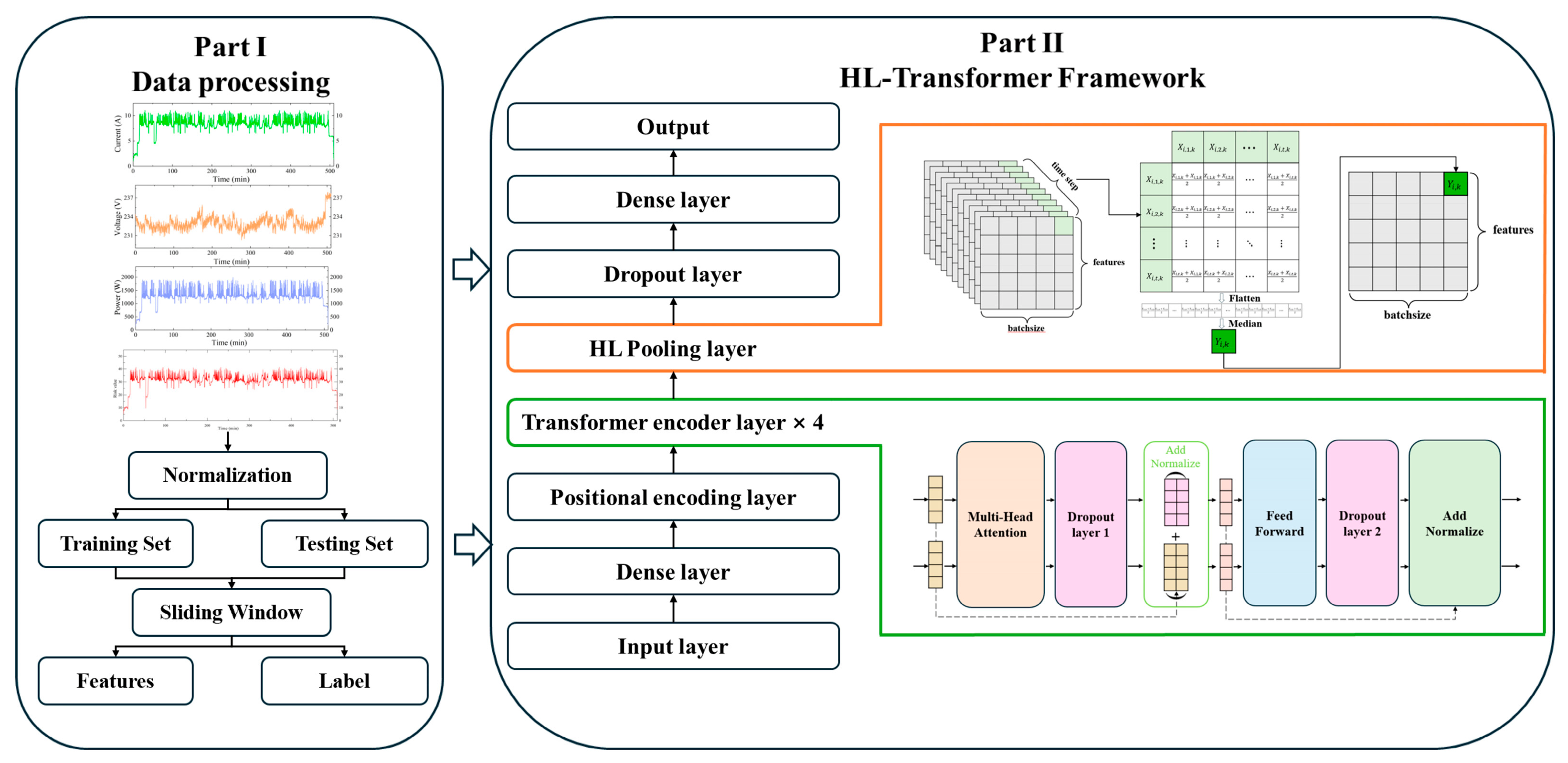
The proposed HL-Transformer-based electrical risk prediction framework consists of two main components, data preprocessing and the HL-Transformer model, as shown in Figure 1. In the data preprocessing stage, raw electrical parameters are collected, normalized, and transformed into sliding-window input sequences. These steps ensure that the model input reflects the temporal evolution of electrical monitoring variables.

The core of the proposed framework is the HL-Transformer model. In this model, a temporal pooling operator based on the HL estimator is designed and embedded into the Transformer architecture. This operator is referred to as the HL-Pooling layer. Its main role is to aggregate encoded temporal representations in a robust manner before the final prediction layer.

The proposed HL-Pooling layer differs from conventional pooling and existing robust aggregation operations in both its statistical form and its role in the network. Average pooling aggregates all temporal responses with equal weights, which makes the output vulnerable to extreme observations. Max pooling selects the strongest activation directly, so isolated spikes may dominate the aggregated representation. Median pooling improves robustness by selecting the middle-ranked feature value along the temporal dimension, but it ignores pairwise relationships among temporal representations. Trimmed mean pooling and winsorized aggregation can reduce the influence of outliers, but their performance depends on a predefined trimming ratio or clipping boundary. Attention-based aggregation can learn adaptive temporal weights, but the learned weights do not inherently provide statistical robustness against extreme sensor disturbances.

In contrast, HL-Pooling first constructs pairwise averages of temporal feature responses and then applies a median operation to these pairwise averages. This procedure combines the smoothing effect of averaging with the outlier resistance of median-based estimation. As a result, the aggregation output is less dominated by isolated spikes than max pooling and less biased by extreme values than average pooling. Since no distributional assumption or manually tuned rejection threshold is required, HL-Pooling is more suitable for noisy electrical monitoring data, where abnormal pulses, sensor drift, and non-Gaussian perturbations may appear unpredictably.

Given the encoder output tensor $H\in {\mathbb{R}}^{B\times T\times D}$, where $B$ is the batch size, $T$ is the temporal length, and $D$ is the feature dimension, the HL-Pooling operation is defined as follows:

$$z_{b,d}=median\left\{{\displaystyle \frac{H_{b,i,d}+H_{b,j,d}}{2}},1\le i\le j\le T\right\}$$

(3)

where $H_{b,i,d}$ and $H_{b,j,d}$ denote the values of the $d$-th hidden feature dimension of the $b$-th sample at time steps $i$ and $j$, respectively. The pooled vector $z_b$ is then passed to the fully connected prediction head to obtain the predicted electrical fire risk value.

In addition, HL-Pooling has translation invariance. When all temporal feature values are shifted by a constant, the pooled result shifts by the same constant:

$$HL\left(X+c\right)=H\left(X\right)+c$$

(4)

This property ensures that the HL-Pooling result shifts linearly with the data, maintaining consistency under global displacements—an essential characteristic for temporal modeling under varying baselines. As illustrated in Figure 1, the HL-Pooling layer is inserted immediately after the final Transformer encoder block and before the fully connected prediction head. In this position, the Transformer encoder first transforms the input sequence into high-level temporal representations through self-attention, positional encoding, residual connections, and feed-forward transformations. The HL-Pooling layer then aggregates these encoded temporal representations along the time dimension and produces a robust fixed-length feature vector for the final prediction layer.

This position was selected because it corresponds to the transition from sequence-level representation learning to prediction-level feature compression. If HL-Pooling were applied before the Transformer encoder, the temporal sequence would be compressed too early, and the self-attention mechanism would not be able to fully model long-range temporal dependencies. If it were applied after the fully connected prediction head, the abnormal temporal activations would already have been propagated into the final prediction mapping, which would weaken the intended robust aggregation effect. Therefore, placing HL-Pooling after the Transformer encoder is the most suitable choice in the proposed architecture, because it preserves the ability of the encoder to learn temporal dependencies while suppressing abnormal activations before final risk prediction.

3.4. Dataset Preparation and Preprocessing

To validate the proposed HL-Transformer-based electrical fire risk prediction model, this study used real-world monitoring data collected from an intelligent fire alarm system deployed at the Chongqing Tobacco Logistics Distribution Center in China. The system continuously records key electrical parameters of the distribution room, including current, voltage, and power, together with a computed fire risk value. The fire risk value is derived from a quantitative risk assessment algorithm that estimates the current fire hazard level based on real-time operating conditions.

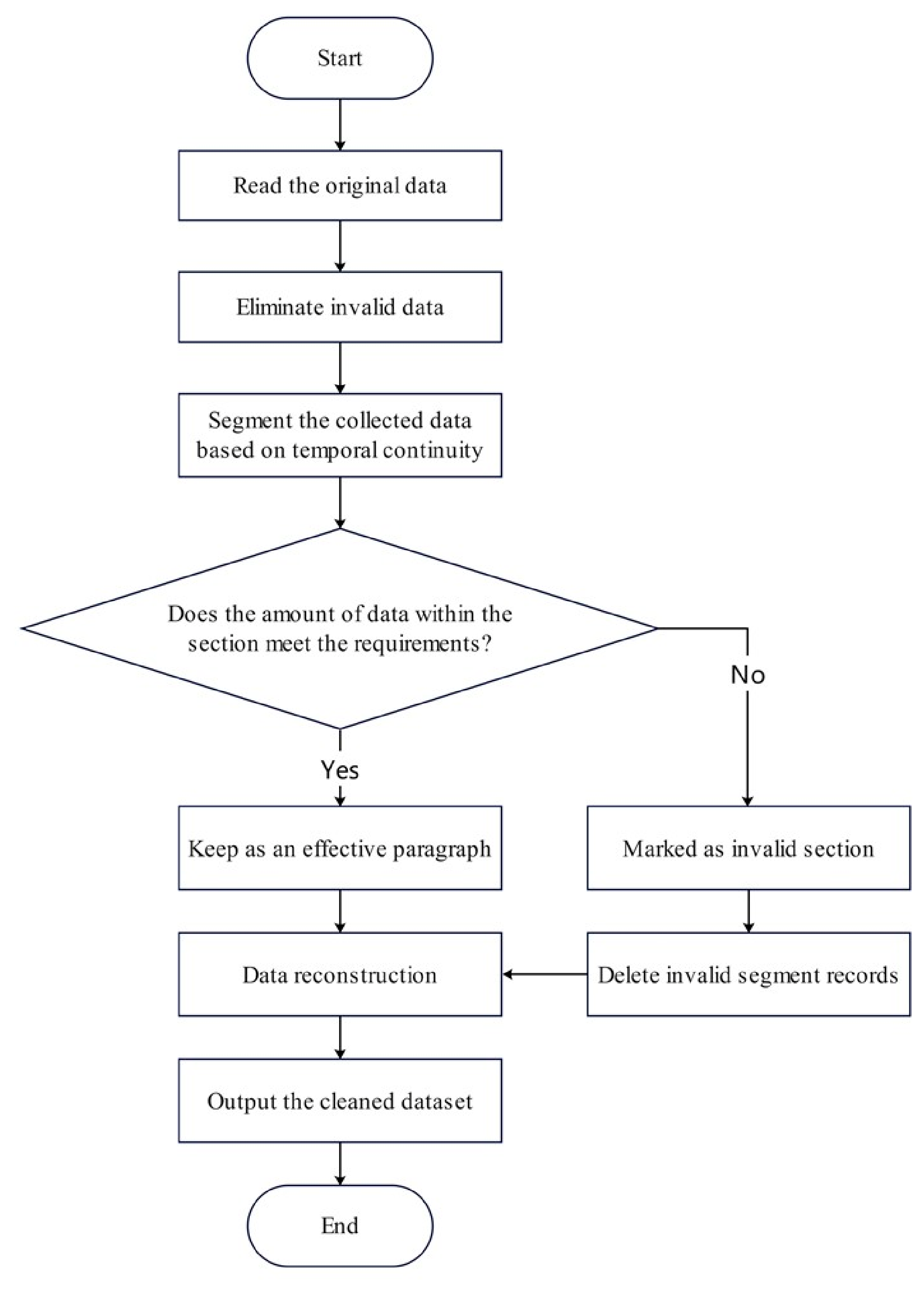
The original dataset spans 23 consecutive days, from 22 March to 13 April, and contains more than 500,000 records. To ensure data quality, invalid entries, such as those recorded during power-off periods, were removed. Abnormal records caused by device malfunction or manual operation errors were also identified and excluded using rule-based filtering and statistical anomaly detection. The overall data processing procedure is shown in Figure 2.

It should be noted that the preprocessing procedure did not aim to remove all abnormal fluctuations from the monitoring sequence. The removed records mainly corresponded to invalid measurements, power-off periods, device malfunctions, communication errors, or obvious manual operation errors that could not represent normal sensor acquisition or meaningful fault evolution. In contrast, operational fluctuations and physically plausible abnormal variations were retained as part of the real-world monitoring sequence. Therefore, the preprocessing step was intended to improve data validity rather than to construct an ideally clean dataset.

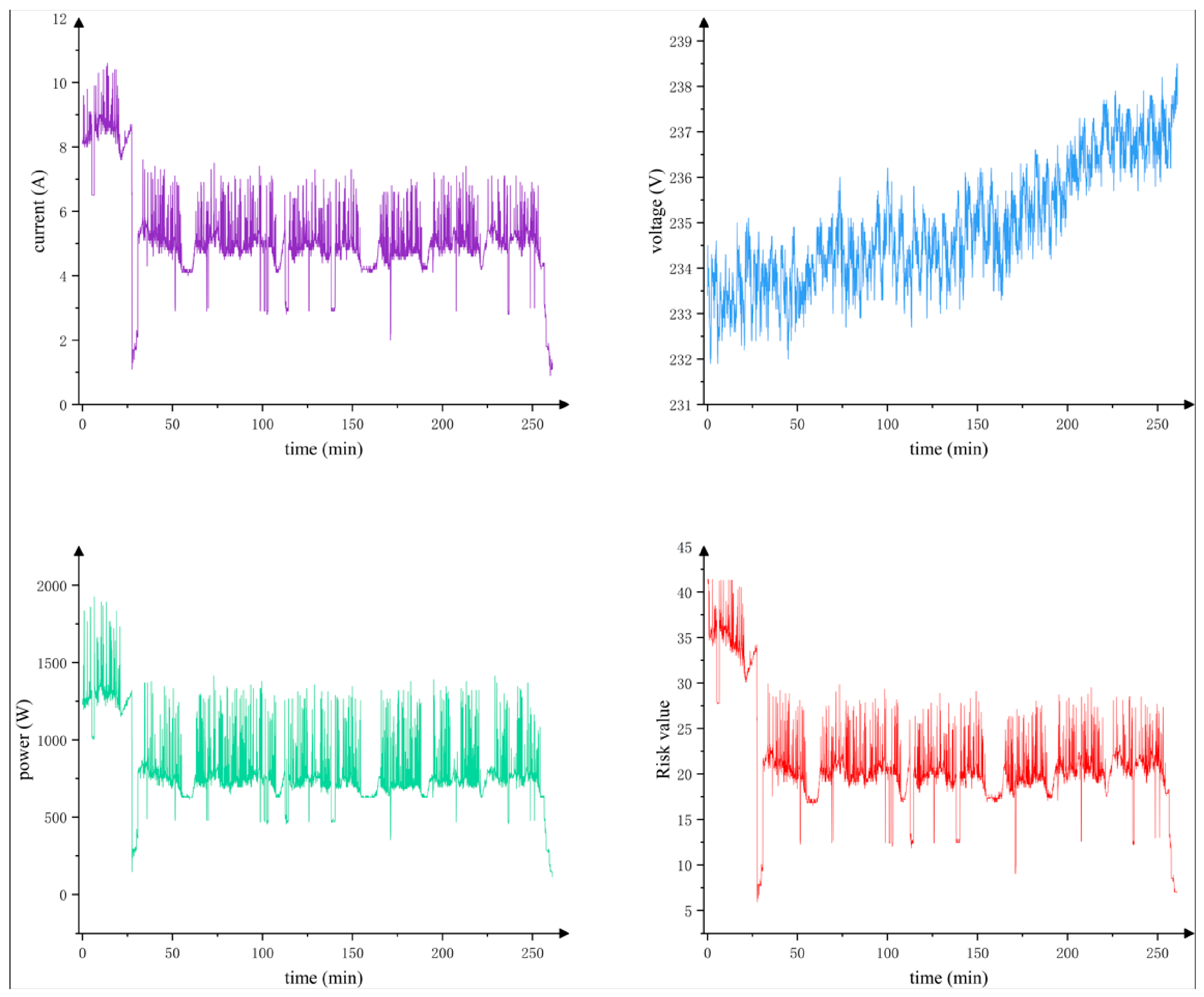
After preprocessing, the dataset was segmented into 11 distinct operational periods, yielding more than 90,000 valid records for model training and evaluation. In this study, the main electrical fire risk prediction experiment focused on the records collected on 22 March 2022. This subset contains 4482 samples with a sampling interval of 5 s. The selected multivariate time series includes key electrical parameters and the corresponding fire risk values. These variables jointly describe the temporal evolution of the electrical system operating state and provide the basis for subsequent time-series forecasting. The raw multivariate time series is shown in Figure 3.

The temporal profiles in Figure 3 show that the current, voltage, and power sequences fluctuate evidently during the observation period, indicating that the operating state of the electrical system changes dynamically rather than remaining at a fixed level. The fire risk value also varies with the evolution of the monitoring parameters, suggesting that risk prediction should consider the temporal dependence among historical observations.

The local fluctuations in the multivariate sequences further indicate the presence of short-term operational variations in real monitoring data. These variations may be related to load switching, sensor disturbance, communication errors, or normal changes in equipment operation. If the encoded temporal features are aggregated directly by average pooling or max pooling, such local fluctuations may bias the final representation or cause isolated high-response points to be overemphasized. Therefore, a robust temporal aggregation module is needed to obtain a more stable representation of the monitoring sequence for electrical fire risk prediction.

It should be noted that the real-world electrical fire monitoring dataset used in this study covers a short-term observation period from 22 March to 13 April 2022. Therefore, this dataset mainly reflects the load characteristics and operating conditions during this period and cannot fully represent seasonal variations in electrical loads. The March 22 subset was selected as the primary case because it contains relatively complete multivariate monitoring records and clear temporal variations suitable for model comparison. Cross-seasonal generalizability was therefore not treated as a fully verified conclusion in this study.

To avoid temporal leakage in the time-series forecasting task, the dataset was divided strictly according to chronological order rather than by random sampling. The earliest portion of the sequence was used for model training, the subsequent portion was used for validation, and the latest portion was reserved as the independent testing set. Specifically, the first 72% of the samples were used for training, the following 8% were used for validation, and the final 20% were used for testing. The same chronological splitting strategy was applied to all compared models to ensure a fair evaluation.

Data normalization was also performed in a leakage-free manner. Specifically, the StandardScaler method from the Scikit-learn library was fitted only on the training subset. The mean and standard deviation estimated from the training subset were then fixed and applied to transform the validation and testing subsets. This procedure ensured that information from the validation and testing periods was not used during preprocessing. The standardization is computed using the following formula:

$$z={\displaystyle \frac{x-\mu }{\sigma }}$$

(5)

where $x$ represents the original data value; $\mu$ is the mean of the original dataset; $\sigma$ denotes the standard deviation of the dataset; $z$ is the standardized data value.

After normalization, sliding windows were constructed within each subset separately. No window was allowed to cross the boundary between the training, validation, and testing subsets. This design prevented future observations or adjacent testing-period information from being introduced into the training process. Therefore, the reported testing results reflect the model’s forecasting performance on unseen future time periods.

3.5. Evaluation Metrics

To comprehensively evaluate the performance of the proposed model, four commonly used evaluation metrics were adopted: Mean Squared Error (MSE), Root Mean Squared Error (RMSE), Mean Absolute Error (MAE), and the Coefficient of Determination (R²). MSE and RMSE eliminate the impact of error sign and provide a holistic assessment of the overall deviation between predicted and actual values. MAE reflects the average magnitude of errors, offering an interpretable metric for typical prediction deviation. R² quantifies the proportion of variance in the observed data that is explained by the model, indicating its overall predictive power. The formulas for these metrics are given as follows:

$$MSE={\displaystyle \frac{1}{N}}{\displaystyle \sum _{m=1}^N}({y\left(m\right)-\widehat{y}\left(m\right))}^2$$

(6)

$$RMSE=\sqrt{{\displaystyle \frac{1}{N}}{\displaystyle \sum _{m=1}^N}({y\left(m\right)-\widehat{y}\left(m\right))}^2}$$

(7)

$$MAE={\displaystyle \frac{1}{N}}{\displaystyle \sum _{m=1}^N}\left|y\left(m\right)-\widehat{y}\left(m\right)\right|$$

(8)

$$R^2=1-{\displaystyle \frac{{\sum }_{i=1}^n{(y_i-\widehat{y_i})}^2}{{\sum }_{i=1}^n{(y_i-\overline{y})}^2}}$$

(9)

3.6. Outlier Injection Strategy for Robustness Testing

To evaluate model robustness under controlled contamination conditions, this study adopted a synthetic outlier injection strategy based on multivariate time-series inputs. This procedure was not intended to replace real fault pulses or to assume that real-world disturbances follow an ideal distribution. Instead, it was designed to provide a controlled stress test, in which the outlier ratio and outlier intensity could be varied independently. In this way, the sensitivity of different temporal aggregation modules to abnormal observations could be compared under the same data split, model backbone, and training setting.

For each dataset, the input variable most highly correlated with the target output was first identified through Pearson correlation analysis. Outliers were then injected into this selected input variable to simulate pulse-noise-like disturbances in electrical monitoring data. The injection was conducted after the baseline dataset had been quality-controlled, so that the effect of abnormal contamination could be isolated from invalid records, power-off periods, or device malfunction records.

The outlier generation process is defined as follows:

$$\tilde{x}=x+K\sigma$$

(10)

where $x$ denotes the original value, $\tilde{x}$ denotes the contaminated value, $\sigma$ denotes the standard deviation of the selected input variable, and $K$ is the shift coefficient controlling outlier intensity.

To evaluate model robustness under varying outlier conditions, two controlled testing settings were designed. In the first setting, the outlier intensity was fixed, and the outlier ratio was increased from 0% to 20% in increments of 0.5%. This setting was used to evaluate model sensitivity to the proportion of abnormal observations in the monitoring sequence. In the second setting, the outlier ratio was fixed, and the shift coefficient K was varied from −40 to 40 to simulate different outlier intensities and directions. This setting was used to evaluate whether the model remained stable when the injected abnormal values deviated from the normal data distribution at different magnitudes.

This design enables a controlled assessment of model robustness under different contamination conditions. It should be noted that the synthetic injection strategy does not fully reproduce all possible non-ideal fault-pulse distributions in real monitoring systems. Rather, it provides a repeatable and comparable way to examine how different models respond to abnormal observations with known ratios and intensities. Future work will further validate the proposed method using longer-term monitoring datasets containing naturally occurring disturbance events and real fault pulses.

4. Results

4.1. Experimental Settings

The dataset preparation, preprocessing procedure, evaluation metrics, and outlier injection strategy have been described in Section 3.4, Section 3.5 and Section 3.6. This section reports the experimental settings and prediction results of the proposed HL-Transformer and the compared models.

To ensure fair comparison across different model configurations, all models were trained using the same set of hyperparameters, as summarized in

Table 1. Hyperparameter settings.

Input Length	Optimizer	Loss Function	Epochs	Batch_Size	Validation_Split
32	Adam	MSE	100	64	0.1

.

4.2. Results with Sensitivity Analysis

4.2.1. Performance Comparison of Temporal Aggregation Modules

To further isolate the contribution of the temporal aggregation module, this study conducted an ablation experiment by replacing only the pooling layer while keeping the Transformer backbone, input length, training strategy, data split, and evaluation metrics unchanged. In addition to conventional Max Pooling and Average Pooling, two robust aggregation baselines, Median Pooling and Winsorized Mean Pooling, were added for comparison. This design allows a more direct evaluation of whether the performance differences are caused by the temporal aggregation module itself rather than by other architectural changes.

As shown in

Table 2. Ablation results of different temporal aggregation modules on the original electrical fire risk test set.

Pooling Strategy	MSE	RMSE	MAE	R2
Max Pooling	8.268	2.875	2.836	0.509
Average Pooling	2.325	1.525	1.439	0.862
Median Pooling	0.005	0.071	0.038	0.9997
Winsorized Mean Pooling	0.007	0.082	0.030	0.9996
HL-Pooling	2.037	1.427	1.376	0.879

, different aggregation modules produced different prediction results on the original electrical fire risk test set. Median Pooling and Winsorized Mean Pooling achieved the lowest errors under clean data conditions. Specifically, Median Pooling obtained an MSE of 0.005 and an R² of 0.9997, while Winsorized Mean Pooling obtained an MSE of 0.007 and an R² of 0.9996. These results indicate that median-type and clipped-mean aggregation methods can provide strong fitting capacity when the monitoring data are weakly disturbed.

Compared with conventional pooling operations, HL-Pooling still achieved better performance than Average Pooling and Max Pooling. The MSE of HL-Pooling was 2.037, which was lower than that of Average Pooling and Max Pooling. Specifically, the MSE reduction relative to Max Pooling was 75.4%, calculated as ${\displaystyle \frac{8.268-2.037}{8.268}}\times 100\%$, while the reduction relative to Average Pooling was 12.4%. This result confirms that HL-Pooling is more suitable than conventional mean- or extreme-value aggregation within the same Transformer backbone. However, the added robust baselines also show that HL-Pooling is not the best choice under all clean-data conditions. Therefore, its value should be interpreted together with its robustness under contaminated inputs rather than only by clean-data fitting accuracy.

The performance difference between HL-Pooling and Max Pooling should not be interpreted simply as the consequence of selecting a more robust estimator. The two pooling strategies transmit different types of temporal information to the prediction head. Max Pooling retains only the largest activation in each feature dimension. Therefore, when a transient spike or a short-duration disturbance produces an abnormally high encoded response, this single time step can dominate the final representation, while the remaining temporal evolution is largely ignored. This behavior is unfavorable for electrical fire risk forecasting, because the risk state is usually related to the cumulative evolution of multiple electrical variables rather than to one isolated high-response point.

In contrast, HL-Pooling constructs pairwise averages across temporal representations and then takes their median. This operation does not simply discard high values. Instead, it redistributes the influence of each time step through pairwise combinations and then selects a central tendency from these combinations. As a result, isolated abnormal activations have limited influence unless they are supported by a broader portion of the sequence. This property is more consistent with electrical fire risk evolution, where meaningful risk increases are usually reflected by sustained or repeatedly supported temporal patterns rather than by a single extreme sensor response.

4.2.2. Robustness Validation of Temporal Aggregation Modules

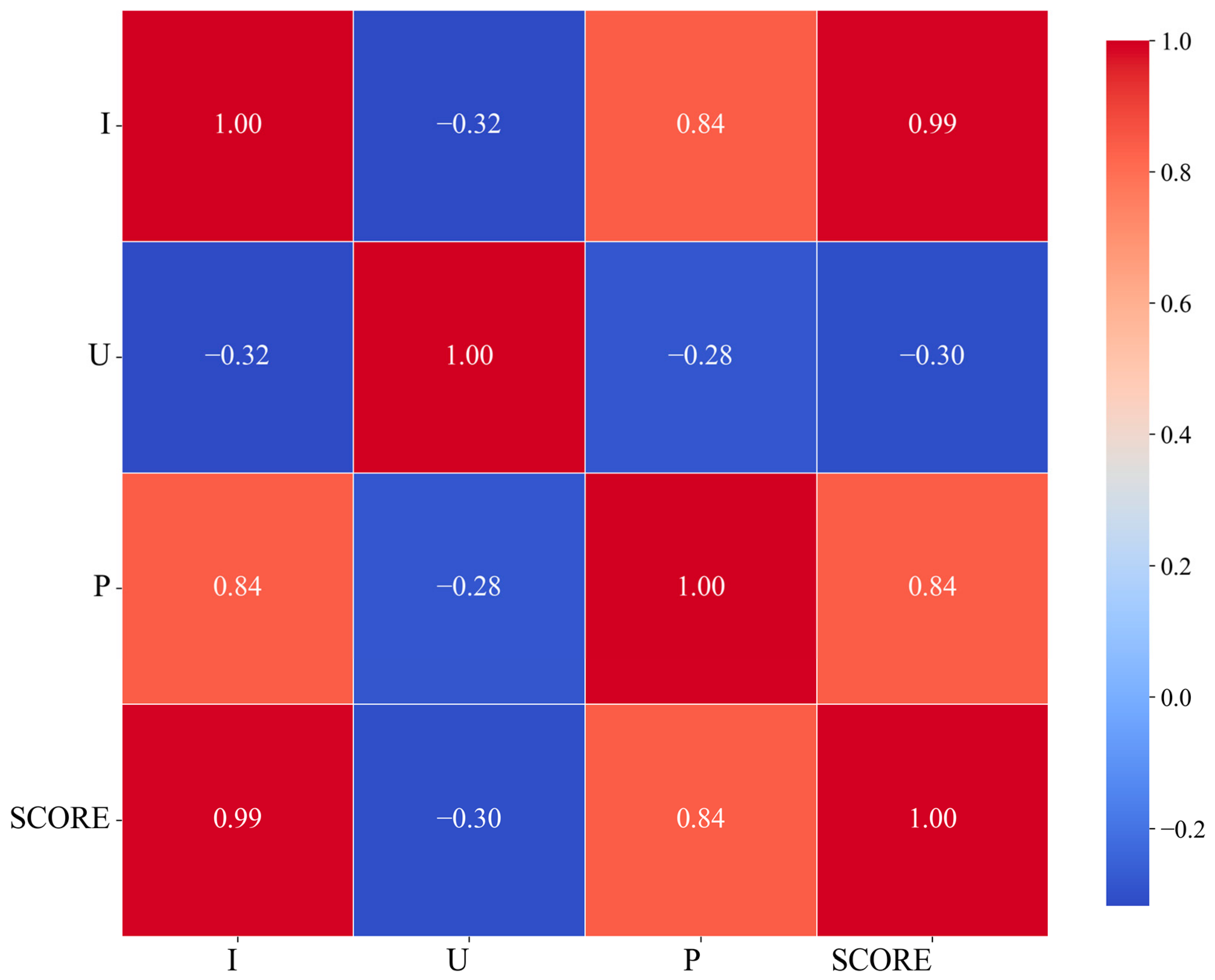
To assess the robustness of different temporal aggregation modules under outlier-contaminated conditions, this study first identified the input variable most relevant to the fire risk value. Pearson correlation analysis was used to measure the relationship between each input variable and the prediction target. As shown in Figure 4, current showed the strongest correlation with the fire risk value. Therefore, the current sequence was selected as the injection target for simulated outliers in the subsequent robustness experiments.

Based on the selected injection variable, five temporal aggregation modules were compared under outlier-contaminated test conditions, including Max Pooling, Average Pooling, Median Pooling, Winsorized Mean Pooling, and HL-Pooling. The Transformer backbone, input length, training strategy, data split, and evaluation metrics were kept consistent. Only the temporal aggregation module was changed. This setting ensures that the observed performance differences mainly come from the aggregation operation rather than from other architectural or training factors.

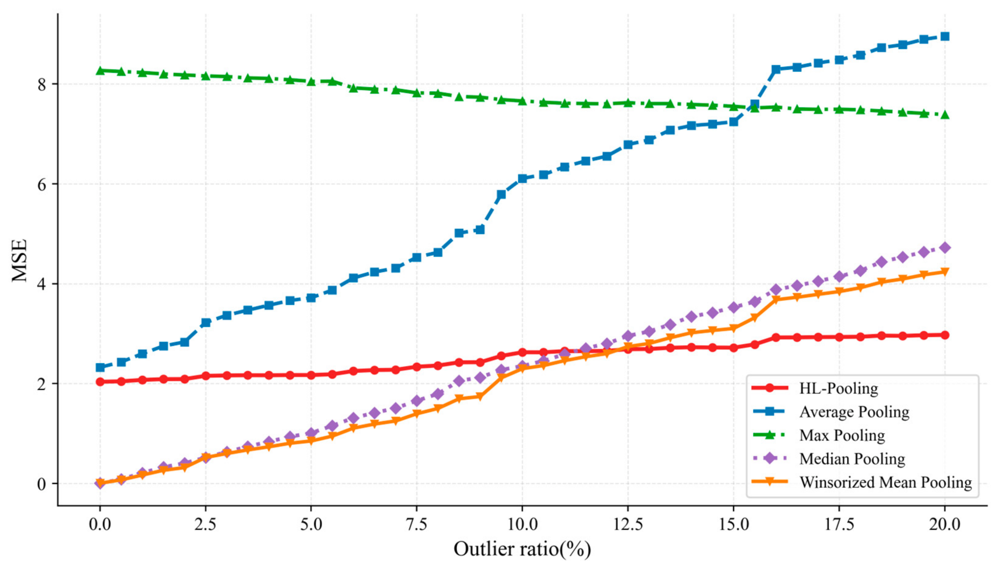
First, the outlier ratio was gradually increased from 0 to 20%, while the outlier intensity was kept fixed. As shown in Figure 5, different aggregation modules exhibited different sensitivities to increasing outlier ratios. Median Pooling and Winsorized Mean Pooling achieved very low errors under clean or weakly contaminated conditions. However, their prediction errors increased more rapidly as the outlier ratio increased. When the outlier ratio increased to 20%, the MSE values of Median Pooling and Winsorized Mean Pooling increased to 4.725 and 4.236, respectively. In contrast, HL-Pooling showed a smoother error trend, and its MSE increased only from 2.037 to 2.975. At the 20% outlier ratio, HL-Pooling achieved the lowest MSE among the five aggregation modules. This result suggests that HL-Pooling is more stable when the monitoring data contain a relatively high outlier ratio.

The main information conveyed by this figure is the change rate of prediction error as the outlier ratio increases. A rapidly increasing error curve indicates that the aggregation module is sensitive to accumulated abnormal points in the input sequence. In contrast, a smoother error curve indicates that the model can maintain a more stable temporal representation under increasing contamination. From this perspective, the advantage of HL-Pooling lies in its smaller performance degradation, rather than only in its absolute error under clean data. This point is important for electrical fire monitoring because sensor sequences may contain repeated short-term disturbances in actual operation. A forecasting model used in this scenario should avoid sharp error growth when abnormal observations become more frequent.

The representative numerical results are summarized in

Table 3. Robustness comparison of different temporal aggregation modules under increasing outlier ratios.

Aggregation Module	MSE at 0%	MSE at 5%	MSE at 10%	MSE at 15%	MSE at 20%
Max Pooling	$8.268$	$8.050$	$7.658$	$7.550$	$7.386$
Average Pooling	$2.325$	$3.718$	$6.108$	$7.242$	$8.954$
Median Pooling	$0.005$	$1.011$	$2.353$	$3.527$	$4.725$
Winsorized Mean Pooling	$0.007$	$0.851$	$2.299$	$3.104$	$4.236$
HL-Pooling	$2.037$	$2.171$	$2.628$	$2.720$	$2.975$

. These results provide quantitative support for the trend observed in Figure 5. Average Pooling showed a clear error increase as the outlier ratio increased, indicating that equal-weight aggregation can be biased when abnormal observations become more frequent. Max-Pooling maintained a relatively high error level across all ratios. This result can be explained by its extreme-value selection mechanism. Once a transient disturbance produces the largest encoded activation in a feature dimension, Max-Pooling directly transfers this isolated response to the prediction head. Therefore, the final representation may be dominated by a short-duration abnormal point rather than by the overall temporal evolution of the monitoring sequence. Median Pooling and Winsorized Mean Pooling performed well at low outlier ratios, but their errors increased more rapidly under higher contamination levels. By contrast, HL-Pooling maintained a more stable error level across the tested ratios because its pairwise-average-and-median operation reduces the dominance of isolated abnormal activations while still preserving sequence-level temporal information.

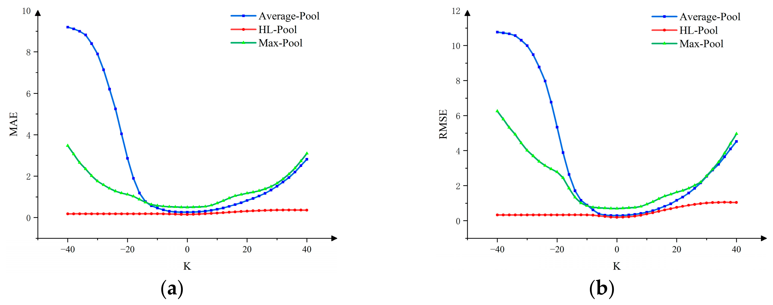
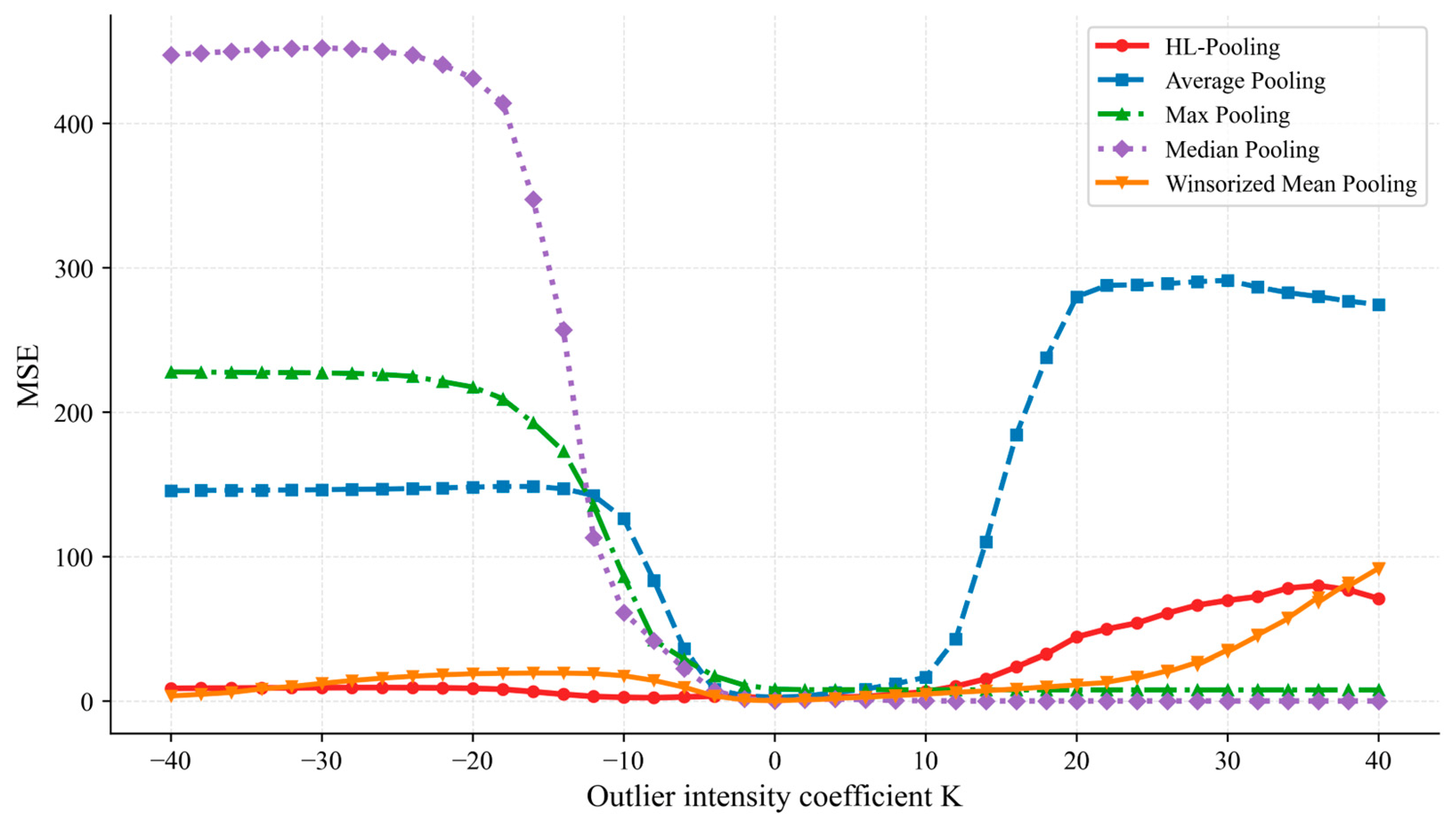
The models were also evaluated under different outlier intensity coefficients with the outlier ratio fixed at 5%. As shown in Figure 6, the results present a more complex pattern. No single robust aggregation module dominated all intensity settings. Median Pooling performed well under positive outlier shifts but degraded severely under extreme negative shifts. For example, when K was −40, the MSE of Median Pooling increased to 447.503, indicating strong sensitivity to negative extreme deviations. Winsorized Mean Pooling showed better stability under K = −40, with an MSE of 3.562, but its error increased substantially when the positive outlier intensity became large. At K = 40, its MSE increased to 91.791. HL-Pooling did not achieve the lowest error under all intensity settings, but it avoided the severe negative-shift failure observed in Median Pooling and showed a more balanced response to different outlier directions.

The figure should therefore be interpreted from both the direction and the magnitude of the injected disturbance. The results indicate that the robustness of a pooling operation depends not only on whether it is based on a robust statistic, but also on how the aggregation rule responds to the distributional position of abnormal temporal responses. HL-Pooling did not dominate all intensity settings, but it avoided severe performance collapse under some extreme shift conditions and showed a more balanced response across different outlier directions. This observation helps define the practical scope of the proposed method. HL-Pooling is more suitable for monitoring conditions with frequent abnormal observations and moderate-to-high contamination ratios, while additional anomaly screening or robust loss functions may still be required when extremely large amplitude shifts occur.

Table 4. Robustness comparison of different temporal aggregation modules under representative outlier intensity coefficients.

Aggregation Module	$\mathit{K}=-40$	$\mathit{K}=-20$	$\mathit{K}=0$	$\mathit{K}=20$	$\mathit{K}=40$
Max Pooling	$227.696$	$217.266$	$8.309$	$7.768$	$7.719$
Average Pooling	$145.747$	$148.111$	$2.606$	$279.831$	$274.478$
Median Pooling	$447.503$	$431.128$	$0.300$	$0.086$	$0.086$
Winsorized Mean Pooling	$3.562$	$18.962$	$0.201$	$11.202$	$91.791$
HL-Pooling	$8.816$	$8.834$	$2.171$	$44.167$	$70.857$

provides representative numerical results under selected outlier intensity coefficients. These results further quantify the different sensitivity patterns of the aggregation modules to the direction and magnitude of outlier shifts.

Overall, these robustness experiments provide a more nuanced interpretation of HL-Pooling. Under clean data conditions, Median Pooling and Winsorized Mean Pooling may provide stronger fitting ability. However, under conditions with a high outlier ratio, HL-Pooling exhibits better stability. Under extreme outlier-intensity conditions, different robust estimators show different sensitivity patterns. Therefore, the proposed HL-Pooling should be regarded as a robust aggregation module with better stability under increasing outlier contamination, rather than as a universally optimal pooling method under all disturbance conditions.

4.2.3. Computational Efficiency Analysis of Temporal Aggregation Modules

To evaluate the computational practicality of the proposed HL-Pooling layer, an additional computational efficiency analysis was conducted. All temporal aggregation modules were evaluated under the same Transformer backbone, input length, batch size, training epochs, data split, optimizer, and loss function. The compared aggregation modules included Max Pooling, Average Pooling, Median Pooling, Winsorized Mean Pooling, and HL-Pooling.

From a theoretical perspective, Max Pooling and Average Pooling require only one scan along the temporal dimension, and their pooling complexity is approximately $O\left(BTD\right)$, where $B$, $T$, and $D$ denote the batch size, temporal length, and hidden feature dimension, respectively. Median Pooling and Winsorized Mean Pooling involve sorting operations along the temporal dimension, and their computational complexity is approximately $O\left(BD\cdot T\mathrm{l}\mathrm{o}\mathrm{g}T\right)$. By contrast, HL-Pooling computes pairwise averages among temporal responses and then applies a median operation. Therefore, its theoretical pooling complexity is approximately $O\left(B{T}^{2}D\right)$. In this study, the input window length was 32, meaning that each hidden feature dimension required $32\times 33/2=528$ pairwise averages. Although this operation is more expensive than standard pooling, its computational scale remains limited under the short-window setting used for electrical fire risk prediction.

All pooling variants had the same number of trainable parameters, namely 72,097. This indicates that HL-Pooling did not increase the model size. Therefore,

Table 5. Computational efficiency comparison of different temporal aggregation modules.

Pooling Strategy	Pooling Complexity	Total Training Time (s)	Latency per Sample (ms)	Peak Training Memory (MB)
Max Pooling	O(BTD)	98.802	0.409	662.719
Average Pooling	O(BTD)	102.900	0.362	813.609
Median Pooling	O(BD·TlogT)	108.319	0.817	907.676
Winsorized Mean Pooling	O(BD·TlogT)	111.600	0.402	994.879
HL-Pooling	O(BT2D)	268.326	0.503	1103.691

mainly reports the pooling complexity, total training time, single-sample inference latency, and peak training memory.

As shown in Table 5, HL-Pooling had a higher theoretical complexity and training cost than standard pooling methods because of its pairwise averaging operation. Its total training time was 268.326 s, which was higher than Max Pooling and Average Pooling. However, the online inference latency remained low. The average inference latency of HL-Pooling was 0.503 ms per sample, which was far below the 5 s sampling interval of the electrical fire monitoring data. This result indicates that HL-Pooling increases offline training cost, but its online inference cost remains acceptable for real-time electrical fire monitoring.

4.2.4. Comparison with Representative Time-Series Forecasting Models

To further evaluate the competitiveness of the proposed HL-Transformer, three representative time-series forecasting models, including Informer, Autoformer, and TimesNet, were introduced for comparison. These models have been widely used in time-series forecasting tasks and can provide stronger reference baselines than conventional neural network models. All models were evaluated using the same electrical fire risk dataset, input length, chronological data split, prediction target, and evaluation metrics. The comparison was conducted under three settings: the original test set, the outlier-contaminated test sets with increasing outlier ratios, and the outlier-contaminated test sets with different outlier intensity coefficients.

As shown in

Table 6. Performance of representative forecasting models on the original electrical fire risk test set.

Model	MSE	RMSE	MAE	R2
Informer	0.310	0.557	0.425	0.982
Autoformer	11.277	3.358	2.496	0.331
TimesNet	0.076	0.275	0.196	0.995
HL-Transformer	2.037	1.427	1.376	0.879

, Informer and TimesNet achieved lower prediction errors than HL-Transformer on the original electrical fire risk test set. Specifically, TimesNet obtained the lowest MSE of 0.076 and the highest R² of 0.995, while Informer obtained an MSE of 0.310 and an R² of 0.982. By comparison, HL-Transformer obtained an MSE of 2.037 and an R² of 0.879. This result indicates that advanced forecasting architectures can provide stronger fitting capacity when the monitoring data are relatively clean and weakly disturbed. Therefore, HL-Transformer should not be interpreted as universally superior to all representative forecasting models under clean-data conditions.

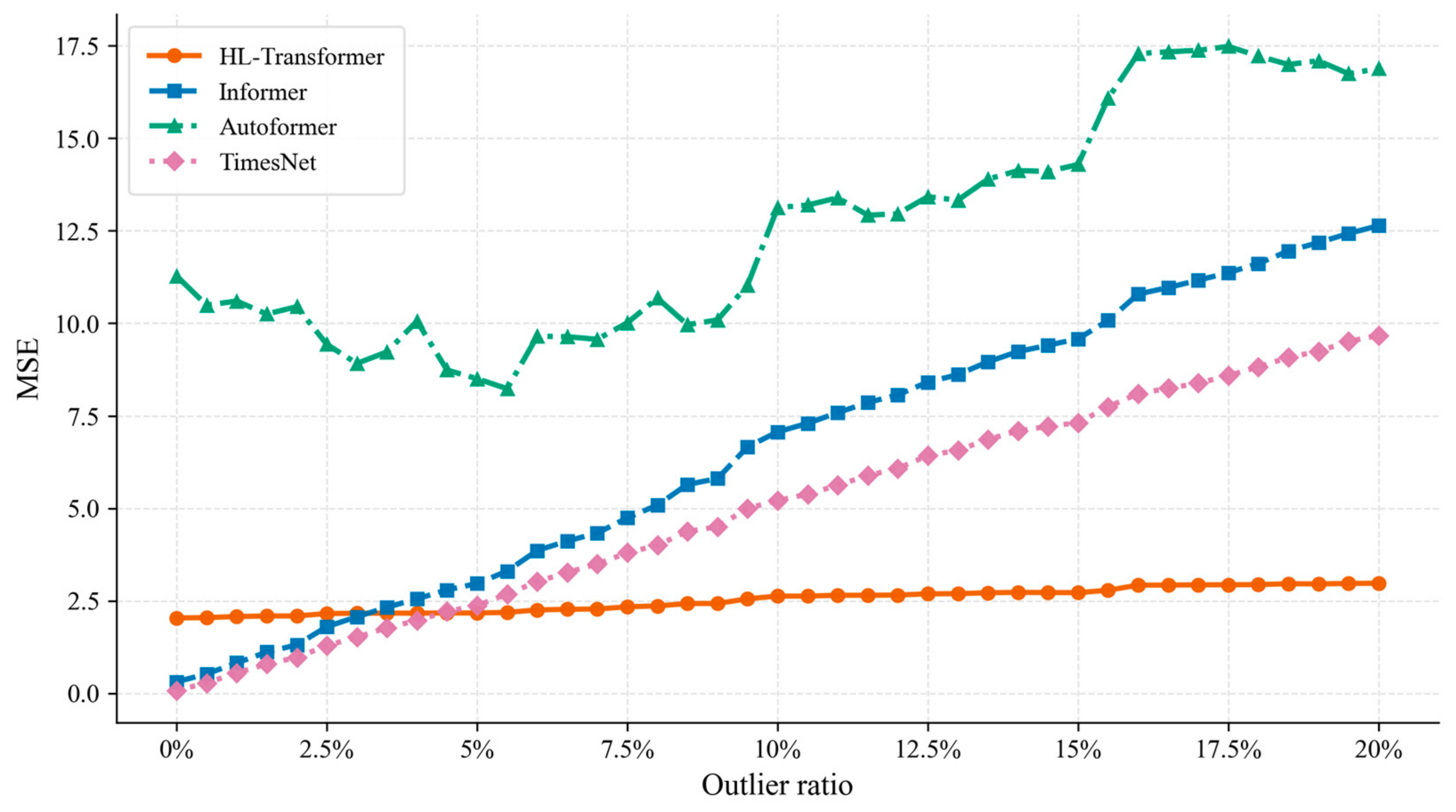
Although Informer and TimesNet performed better on the original test set, their errors increased rapidly when the outlier ratio increased. As shown in Figure 7, the MSE values of Informer and TimesNet increased sharply as the outlier ratio increased from 0 to 20%. Informer increased from 0.310 to 12.638, and TimesNet increased from 0.076 to 9.674. In contrast, HL-Transformer showed a much smoother error trend, with its MSE increasing only from 2.037 to 2.975. This result indicates that HL-Transformer has a more stable response when the monitoring data contain an increasing outlier ratio.

The representative numerical results under different outlier ratios are summarized in

Table 7. MSE results of HL-Transformer and representative forecasting models under increasing outlier ratios.

Model	$\mathbf{M}\mathbf{S}\mathbf{E} \mathbf{a}\mathbf{t} 0\%$	$\mathbf{M}\mathbf{S}\mathbf{E} \mathbf{a}\mathbf{t} 5\%$	$\mathbf{M}\mathbf{S}\mathbf{E} \mathbf{a}\mathbf{t} 10\%$	$\mathbf{M}\mathbf{S}\mathbf{E} \mathbf{a}\mathbf{t} 15\%$	$\mathbf{M}\mathbf{S}\mathbf{E} \mathbf{a}\mathbf{t} 20\%$
Informer	$0.310$	$2.966$	$7.066$	$9.582$	$12.638$
Autoformer	$11.277$	$8.502$	$13.128$	$14.292$	$16.888$
TimesNet	$0.076$	$2.371$	$5.210$	$7.314$	$9.674$
HL-Transformer	$2.037$	$2.171$	$2.628$	$2.720$	$2.975$

. As shown in Table 7, TimesNet and Informer had clear advantages under clean or weakly contaminated conditions, but their errors increased more rapidly under higher outlier ratios. Autoformer showed a relatively high error level across the tested conditions. Average Pooling was also sensitive to increasing outlier ratios, while Max Pooling maintained a high error level. Compared with these methods, HL-Transformer did not achieve the lowest error under clean data conditions, but it showed smaller performance degradation when the outlier ratio increased. This result is consistent with the design purpose of HL-Pooling, which aims to improve the stability of temporal aggregation under noisy monitoring conditions.

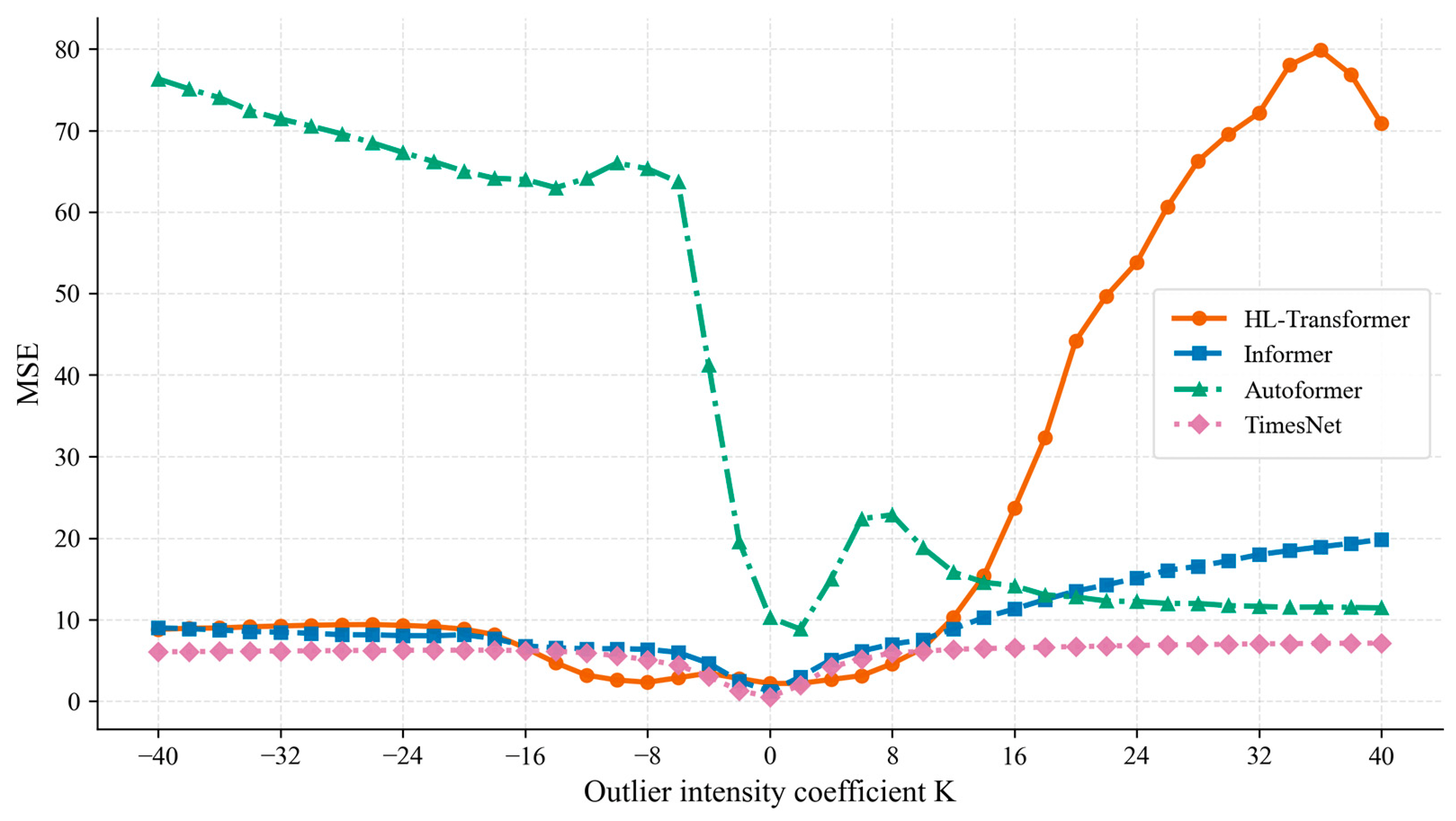
The models were also evaluated under different outlier intensity coefficients with the outlier ratio fixed at 5%. As shown in Figure 8, the results present a more complex pattern. TimesNet maintained lower MSE values over a wider range of intensity coefficients, indicating its strong resistance to amplitude-shift interference in this experimental setting. By contrast, HL-Transformer did not dominate all intensity conditions. In particular, its error increased under large positive outlier shifts. This result suggests that HL-Transformer is not universally superior under all disturbance types.

The representative numerical results under different outlier intensity coefficients are shown in

Table 8. MSE results of HL-Transformer and representative forecasting models under representative outlier intensity coefficients.

Model	$\mathbf{K}=-40$	$\mathbf{K}=-20$	$\mathbf{K}=0$	$\mathbf{K}=20$	$\mathbf{K}=40$
Max Pooling	$227.696$	$217.266$	$8.309$	$7.768$	$7.719$
Average Pooling	$145.747$	$148.111$	$2.606$	$279.831$	$274.478$
Informer	$8.989$	$8.144$	$1.185$	$13.509$	$19.854$
Autoformer	$76.324$	$64.997$	$10.263$	$12.783$	$11.440$
TimesNet	$6.052$	$6.256$	$0.518$	$6.694$	$7.120$
HL-Transformer	$8.816$	$8.834$	$2.171$	$44.167$	$70.857$

. As shown in Table 8, TimesNet achieved relatively low MSE values at both negative and positive intensity settings. Informer showed moderate errors under negative shifts, but its error increased under larger positive shifts. Autoformer had relatively high errors under negative shifts and at K = 0. Max Pooling showed lower errors under positive shifts but had high errors under negative shifts. Average Pooling was highly sensitive to both negative and positive large shifts. HL-Transformer showed moderate errors under negative shifts, but its error increased under positive extreme shifts. These results indicate that different forecasting architectures and aggregation mechanisms have different sensitivities to the direction and magnitude of outlier shifts.

Overall, the comparison with representative time-series forecasting models provides a more balanced understanding of the proposed method. Informer and TimesNet show stronger fitting ability on relatively clean data, and TimesNet also performs well under different outlier intensity coefficients. However, when the outlier ratio increases, HL-Transformer shows a more stable error trend and smaller performance degradation. Therefore, the main value of HL-Transformer is not universal clean-data superiority, but robust temporal aggregation under noisy electrical fire monitoring conditions, especially when the monitoring sequence contains an increasing proportion of abnormal observations.

4.3. Generalization Validation of HL-Pooling

In this section, this study systematically validates the generalization capability of the proposed HL-Pooling layer through cross-dataset validation and module transferability experiments.

4.3.1. Transferability Verification on the Public Dataset

To assess the transferability of the proposed model, a number of validation experiments are conducted using the publicly available ETTh1 dataset. The ETT dataset records temperature measurements from power transformers and is available in two sampling resolutions: hourly (ETTh1 and ETTh2) and every 15 min (ETTm1 and ETTm2) [48]. The data spans a two-year period from July 2016 to July 2018. Each dataset contains seven features related to transformer oil temperature and electrical load conditions.

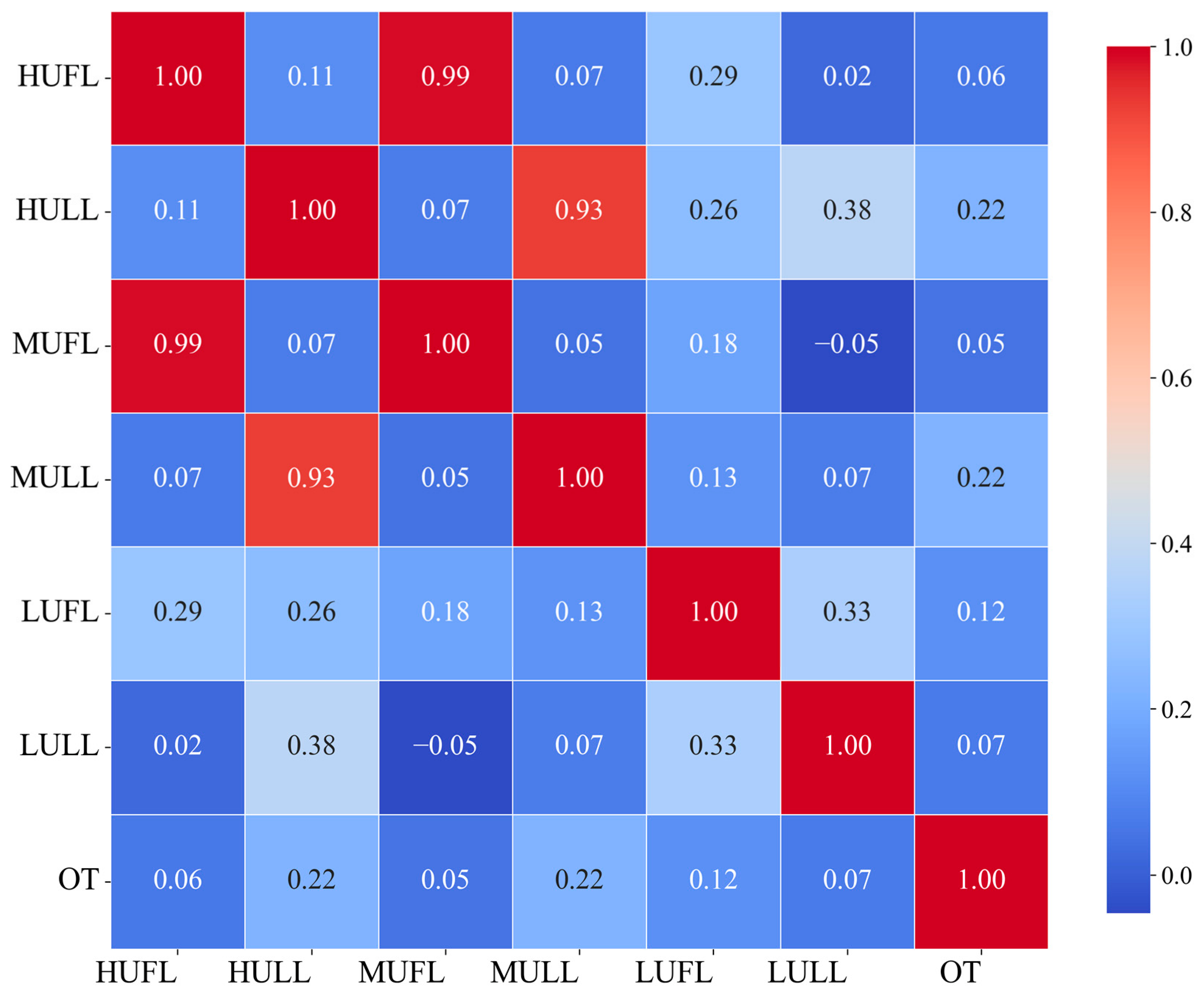
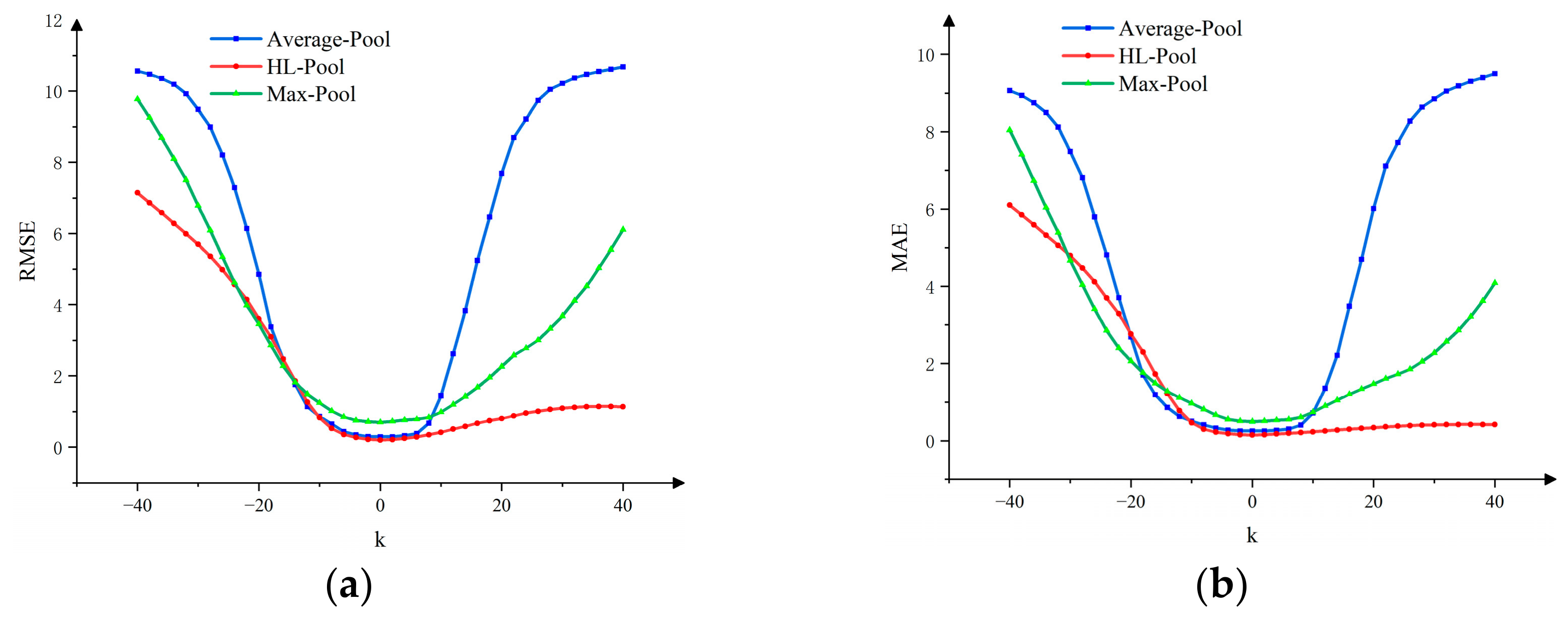
To simulate real-world data contamination scenarios and evaluate the robustness, a correlation analysis is performed to identify the most relevant input features associated with the target variable; see Figure 9. According to the correlation-analysis results, this study selects the HULL and MULL as the top correlated features. Subsequently, synthetic anomalies were injected into the HULL feature column for experimental purposes.

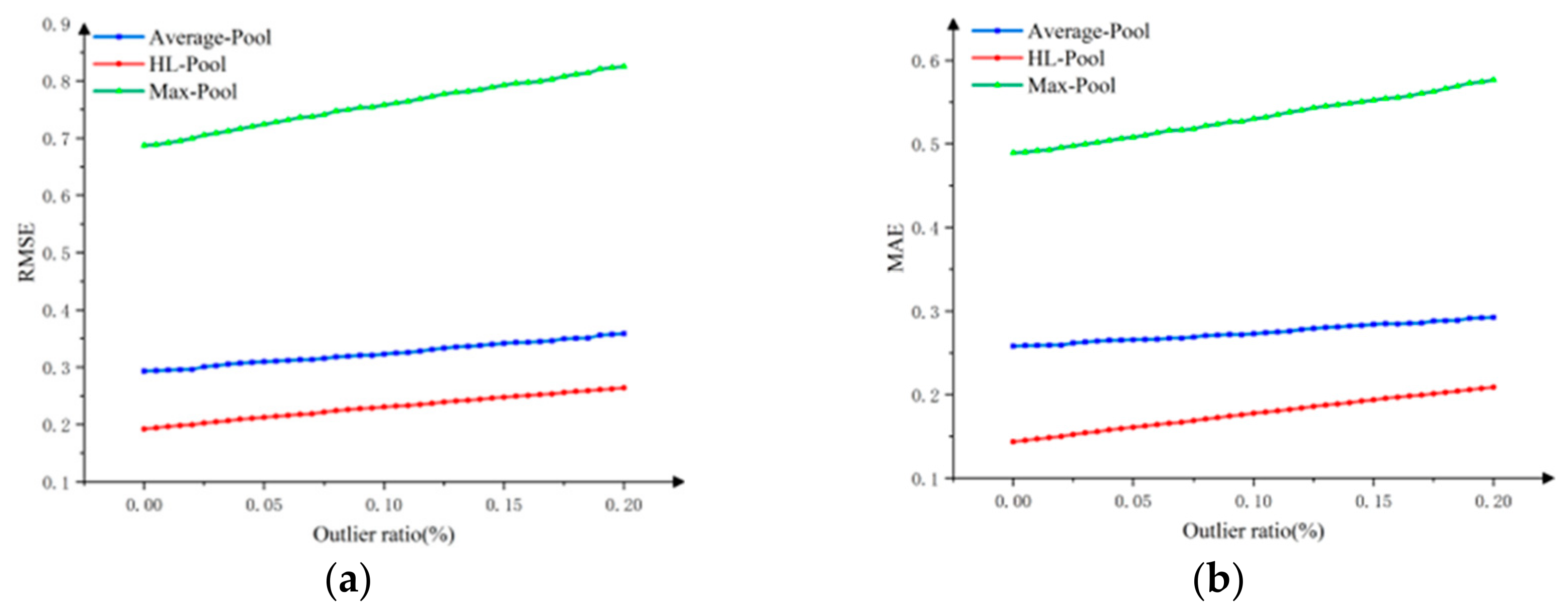
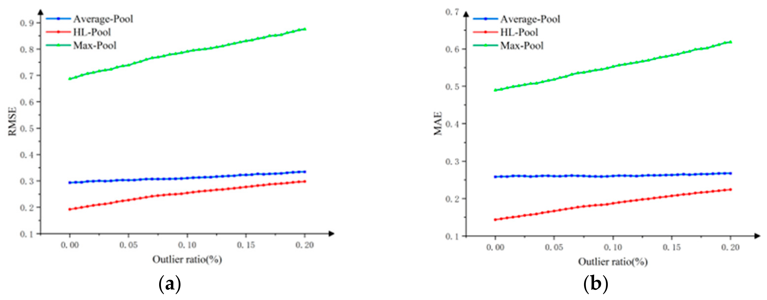
As shown in Figure 10, the performance of HL-Pooling was compared with that of average pooling and max pooling under increasing outlier ratios. HL-Pooling showed smaller error fluctuations and lower RMSE and MAE values than the other two pooling strategies, indicating better robustness when the outlier ratio increased.

Figure 11 shows the changes in RMSE and MAE under different outlier intensity coefficients, with the outlier ratio fixed at 5%. HL-Pooling maintained more stable prediction accuracy when the injected outliers shifted in either the positive or negative direction. Overall, the HL-Pooling demonstrates stronger robustness compared to average pooling and max pooling across a wide range of outlier intensities.

In addition to the above comparison, this study injects outliers into both the HULL and MULL columns using the same outlier generation method to evaluate the robustness of the proposed model when multiple input datasets are simultaneously contaminated. As shown in Figure 12 and Figure 13, the proposed model using HL-Pooling layer still maintained superior robustness and prediction performance under these multi-source outlier conditions.

The ETTh1 robustness figures provide further evidence on whether the observed stability of HL-Pooling is dataset-specific or transferable to another multivariate time-series dataset. The comparison under single-column and multi-column outlier injection indicates that HL-Pooling can still reduce error fluctuation when abnormal observations appear in more than one input variable. This result supports the interpretation that HL-Pooling acts as a general robust temporal aggregation module, rather than as a mechanism tailored only to the electrical fire risk dataset.

4.3.2. Comparative Validation with Baseline Models

To further validate the effectiveness of the proposed HL-Pooling layer, this study conducts comparative experiments using three widely adopted baseline architectures for time series forecasting. The three baseline architectures are CNN-LSTM [49], 1D-CNN [50], and TCN [51]. CNN-LSTM combines 1D convolutional layers for local temporal feature extraction with LSTM layers for long-term dependency modeling, and the pooling layer is placed after the convolutional block for dimensionality reduction. The 1D-CNN model consists of stacked one-dimensional convolutional blocks, where pooling is used to compress intermediate temporal feature representations. TCN is based on dilated causal convolutions, and pooling layers are embedded between residual blocks to reduce computational complexity.

To ensure a fair assessment of the transferability of HL-Pooling, the comparison was designed as a controlled module-replacement experiment. For each baseline architecture, including TCN, CNN-LSTM, and 1D-CNN, the data split, input window length, preprocessing procedure, loss function, optimizer, number of training epochs, batch size, and validation strategy were kept the same. Within each backbone, the convolutional, recurrent, residual, and fully connected layers were kept unchanged, and only the pooling operation was replaced by HL-Pooling, max pooling, or average pooling. Therefore, the reported performance differences within the same backbone mainly reflect the influence of the temporal aggregation module rather than changes in the overall model structure or training setting.

It should also be noted that the objective of this experiment was not to claim that one backbone architecture was universally superior to another. Different backbones naturally have different parameter scales and feature extraction mechanisms. Therefore, the cross-architecture comparison was used only to examine whether HL-Pooling could be transferred to different types of time-series forecasting models. The main evidence for the effectiveness of HL-Pooling comes from the within-backbone comparisons, where the model configuration and training budget were controlled and the pooling layer was the only changed component.

To assess the impact of different pooling strategies within these models, the original pooling operation in each backbone was replaced with HL-Pooling, max pooling, or average pooling, while the remaining model components were kept unchanged. This configuration enables a comprehensive comparison across multiple model architectures and pooling mechanisms, highlighting the general applicability and robustness of HL-Pooling in both convolutional and hybrid sequential modeling tasks. As shown in

Table 9. Comparative results of different pooling methods across baseline models.

Dataset	Model	Metrics	Pooling Layers			IM (%)
			HL	Max	Average
ETTh1	TCN	$R^2$	0.999	0.993	0.975	0.6
		MSE	0.011	0.047	0.132	76.6
		RMSE	0.131	0.282	0.541	53.5
		MAE	0.091	0.266	0.466	65.8
	CNN_LSTM	$R^2$	0.919	0.77	0.835	9.1
		MSE	0.958	2.726	1.963	51.2
		RMSE	0.979	1.651	1.401	30.1
		MAE	0.849	1.356	1.097	22.6
	1D_CNN	$R^2$	0.882	0.514	0.808	8.4
		MSE	1.399	5.766	2.27	38.4
		RMSE	1.183	2.401	1.507	21.5
		MAE	0.905	1.871	1.189	23.9
FIRE RISK	TCN	$R^2$	0.900	0.473	0.885	1.7
		MSE	1.678	1.94	1.827	8.2
		RMSE	1.295	2.979	1.393	7
		MAE	0.897	2.379	0.912	1.6
	CNN_LSTM	$R^2$	0.968	0.931	0.930	3.8
		MSE	0.536	1.15	1.185	61.4
		RMSE	0.732	1.073	1.088	34.1
		MAE	0.493	0.728	0.759	23.5
	1D_CNN	$R^2$	0.486	0.462	0.378	4.9
		MSE	8.661	9.071	10.475	41
		RMSE	2.943	3.012	3.236	6.9
		MAE	1.938	2.262	2.198	11.8

, the $R^2$, MSE, RMSE, and MAE results are provided using different pooling layers, where the improvement rates (i.e., IM) are also provided. The results show that models equipped with HL-Pooling generally achieved lower prediction errors than those using max pooling or average pooling, supporting the robustness and transferability of the proposed HL-Pooling layer.

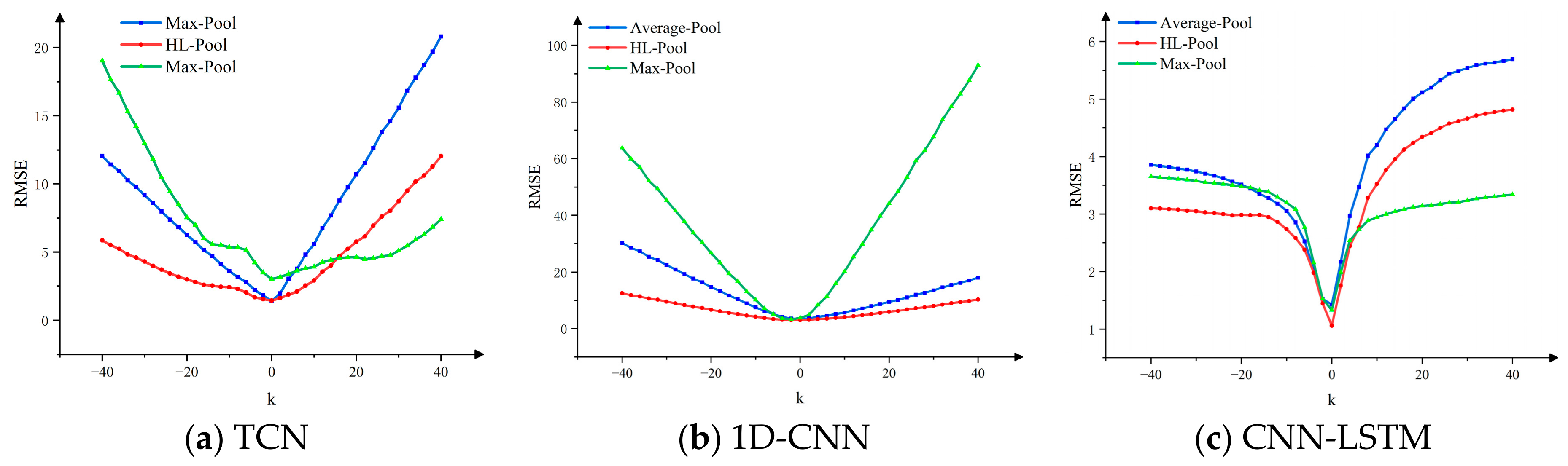
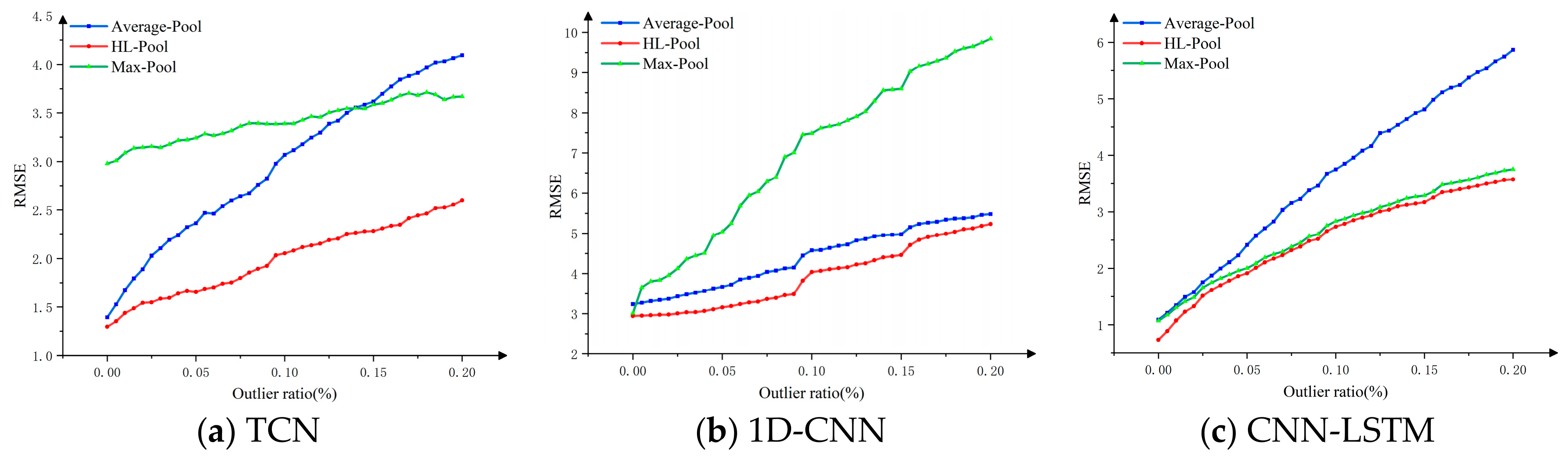
This study further investigated the performance of the three baseline models under different outlier shift coefficients and outlier ratios when different pooling strategies were used. The relevant results are visualized in Figure 14 and Figure 15. Specifically, Figure 14 illustrates the impact of varying shift coefficients on model performance. It is clear that when the $k$ value remains within a relatively small range, models equipped with the HL-Pooling layer consistently achieve lower RMSE values, indicating superior robustness against mild anomalies. However, as the $k$ value increases, the performance of the HL-Pooling layer begins to diverge across different model architectures. The RMSE values exhibit varying trends depending on the underlying model, suggesting that the interaction between model design and outlier intensity is complex. These findings highlight that, while the HL-Pooling layer generally enhances robustness, its effectiveness under severe anomaly conditions is influenced by the specific model structure, necessitating careful model selection and design in real-world applications.

Compared with average pooling and max pooling, the models equipped with HL-Pooling showed more stable RMSE trends under varying outlier ratios. This result suggests that HL-Pooling can reduce performance degradation when abnormal observations become more frequent. The improvement is not only related to the robustness of the HL estimator itself, but also to the way temporal information is aggregated. Average pooling treats all time steps equally and may be biased when contaminated observations accumulate. Max pooling directly selects the strongest activation and may overemphasize isolated spikes. In contrast, HL-Pooling aggregates temporal responses through pairwise averages followed by a median operation, which weakens the effect of isolated abnormal activations while preserving the central tendency of the encoded sequence. Therefore, HL-Pooling provides a more stable temporal representation in anomaly-prone monitoring environments.

5. Discussion

This study proposed an HL-Transformer model for electrical fire risk forecasting under noisy monitoring conditions. The main purpose of the proposed model is not to achieve universal superiority under all data conditions, but to improve the stability of temporal feature aggregation when electrical monitoring sequences contain transient outliers, pulse-type disturbances, or non-Gaussian fluctuations. This distinction is important because electrical fire warning systems are often deployed in environments where sensor readings may be affected by load switching, communication errors, device disturbances, or short-term operational changes. In such cases, a forecasting model should not only fit clean data well, but should also avoid sharp performance degradation when abnormal observations accumulate.

The methodological contribution of this study lies in reformulating the Hodges–Lehmann estimator as a temporal pooling layer for deep time-series forecasting. In the proposed architecture, the Transformer encoder first extracts temporal dependencies from multivariate monitoring data, and the HL-Pooling layer then aggregates the encoded temporal representations before the final prediction head. This design differs from conventional pooling operations. Average pooling assigns equal influence to all temporal responses, so its output may be shifted when contaminated observations become frequent. Max pooling selects the strongest activation in each feature dimension, so one isolated spike may dominate the final representation. This behavior is not well aligned with electrical fire risk evolution, because fire risk is usually associated with cumulative temporal patterns and repeated abnormal support rather than one isolated high-response point. In contrast, HL-Pooling constructs pairwise averages among temporal representations and then applies a median operation. This process reduces the influence of isolated abnormal activations while still preserving the central tendency of the encoded sequence.

The ablation results support this interpretation, but they also show that HL-Pooling should not be regarded as the best aggregation method under all conditions. Under clean data conditions, Median Pooling and Winsorized Mean Pooling achieved lower errors than HL-Pooling. This indicates that some robust aggregation methods can provide stronger fitting capacity when the monitoring data are weakly disturbed. However, their advantage decreased when the outlier ratio increased. When the outlier ratio reached 20%, Median Pooling and Winsorized Mean Pooling showed larger error increases, whereas HL-Pooling maintained a smoother error trend. This result suggests that the value of HL-Pooling is mainly reflected in its smaller performance degradation under increasing contamination, rather than in clean-data fitting alone.

The comparison with representative time-series forecasting models further clarifies the positioning of the proposed method. On the original electrical fire risk test set, TimesNet and Informer achieved lower prediction errors than HL-Transformer, which shows that advanced forecasting architectures may have stronger fitting capacity under relatively clean monitoring conditions. Therefore, the proposed method should not be described as universally superior to current time-series forecasting models. However, when the outlier ratio increased, the errors of Informer and TimesNet increased more rapidly, whereas HL-Transformer showed a more stable response. This finding indicates that the proposed HL-Pooling mechanism is more useful when the monitoring sequence contains an increasing outlier ratio. In this sense, HL-Transformer provides a robustness-oriented complement to high-capacity forecasting models, rather than a direct replacement for all SOTA architectures.

The results under different outlier intensity coefficients also reveal the boundary of the proposed method. HL-Pooling did not dominate all disturbance settings. In particular, the model error increased under severe positive outlier shifts. This suggests that HL-Pooling is more effective in resisting an increasing proportion of abnormal observations than in completely eliminating the influence of extremely large amplitude shifts. This phenomenon is reasonable because HL-Pooling is an aggregation-level robust operation. It can weaken the effect of isolated abnormal activations, but it cannot fully correct severely distorted input distributions before feature extraction. Therefore, when real monitoring data contain extremely large fault pulses, sensor saturation, or systematic drift, additional mechanisms may still be needed. These mechanisms may include adaptive anomaly screening, robust loss functions, uncertainty estimation, or hybrid preprocessing modules.

The computational analysis shows that HL-Pooling introduces additional offline training cost because it computes pairwise averages along the temporal dimension. Its theoretical complexity is higher than standard average pooling and max pooling. The experimental results also show that HL-Pooling required longer training time and higher peak training memory than standard pooling. However, the online inference latency remained low. The average inference latency of HL-Pooling was 0.503 ms per sample, which is far below the 5 s sampling interval of the electrical fire monitoring data used in this study. This indicates that the added computational cost mainly affects offline training, while the online prediction cost remains acceptable for real-time monitoring scenarios. From an engineering perspective, this is important because electrical fire warning systems usually require timely inference after model deployment, whereas model training can be performed offline.

The cross-dataset and transfer experiments provide additional evidence for the modular value of HL-Pooling. The ETTh1 experiments show that the robustness advantage is not limited to the electrical fire risk dataset. The transfer experiments on TCN, CNN-LSTM, and 1D-CNN also show that HL-Pooling can be embedded into different time-series forecasting backbones. This suggests that HL-Pooling is better understood as a portable temporal aggregation module. Its effectiveness depends on the interaction between the aggregation rule, the backbone architecture, and the disturbance pattern in the input sequence. Therefore, future applications should not assume that HL-Pooling will always produce the best result in every model. Instead, it should be evaluated as a robust aggregation option when monitoring data are noisy, non-Gaussian, or prone to transient abnormal observations.

This study also differs from recent visual-language-model and large-language-model studies in fire-risk identification. Recent VLM- and LLM-based studies mainly focus on visual or multimodal scene understanding, such as building fire-hazard recognition, fire-image interpretation, and semantic reasoning from visual information. These methods are valuable when image, video, or spatial context is available. By contrast, the present study focuses on sensor-based electrical fire risk forecasting from multivariate time-series data. The proposed HL-Transformer does not replace VLM-based fire-risk identification methods. Instead, it provides a complementary route for electrical fire early warning, especially when the available information mainly consists of current, voltage, power, and derived risk values. In practical systems, visual inspection methods and sensor-based forecasting methods may be combined to improve the completeness of fire-risk monitoring.

Several limitations remain. The real-world electrical fire monitoring dataset covers only a short observation period from 22 March to 13 April 2022, and the main case study focuses on the 22 March subset. Therefore, the current results cannot fully verify cross-seasonal generalizability. Electrical loads may vary across seasons, working schedules, equipment conditions, and management patterns. A model trained and tested on short-term data may not capture all long-term periodic or seasonal risk patterns. Future work should validate the proposed method using longer monitoring periods, more buildings, and more diverse electrical operating conditions.

Another limitation is that the robustness experiments used controlled synthetic outlier injection. This design was useful for comparing different models under known outlier ratios and intensities, but it cannot fully reproduce all non-ideal fault-pulse distributions in real monitoring systems. Real disturbances may involve correlated multi-variable changes, sensor saturation, long-duration drift, missing values, or complex fault evolution. Future work should incorporate naturally occurring disturbance events and real fault records to further test the robustness of HL-Pooling under more realistic conditions.

The current task is also formulated as continuous risk-value forecasting rather than binary alarm classification. Therefore, this study did not calculate Recall, False Negative Rate, or Precision for fire threshold warnings. These warning-oriented metrics are important for actual fire alarm deployment because the cost of missed alarms is high. However, reliable calculation of these metrics requires validated alarm thresholds and binary event labels. Future studies should combine continuous risk forecasting with threshold calibration, alarm-event labeling, and safety-oriented evaluation metrics. This would make it possible to assess not only prediction error, but also warning performance in practical fire prevention scenarios.

Overall, the proposed HL-Transformer is most suitable for electrical fire monitoring scenarios where multivariate time-series data contain frequent transient disturbances and where stable temporal aggregation is required. Its main strength lies in improving robustness under increasing outlier contamination while maintaining acceptable inference cost. Its main limitations lie in limited validation data, incomplete verification under real fault pulses, and reduced advantage under extremely large amplitude shifts. These findings provide a more balanced understanding of HL-Pooling as a robust and portable aggregation module for noisy time-series forecasting.

6. Conclusions

This study proposed an HL-Transformer model for robust electrical fire risk forecasting under noisy monitoring conditions. The proposed model embeds an HL-Pooling layer based on the Hodges–Lehmann estimator into the Transformer architecture. The HL-Pooling layer aggregates encoded temporal representations by taking the median of pairwise averages, thereby reducing the influence of abnormal temporal activations while preserving the central tendency of the sequence.

The experimental results show that HL-Pooling improved prediction performance compared with conventional average pooling and max pooling within the same Transformer backbone. On the original electrical fire risk test set, HL-Transformer achieved an MSE of 2.037 and an R² of 0.879. The ablation study further showed that Median Pooling and Winsorized Mean Pooling achieved stronger fitting performance under clean data conditions, but their errors increased more rapidly when the outlier ratio increased. In contrast, HL-Pooling maintained a smoother error trend and achieved better stability under conditions with a high outlier ratio. This result indicates that the main advantage of HL-Pooling lies in robust temporal aggregation under contaminated monitoring data, rather than universal superiority under clean data.

The comparison with Informer, Autoformer, and TimesNet further clarified the position of the proposed method. TimesNet and Informer showed stronger fitting capacity on the original test set, but their errors increased more sharply when the outlier ratio increased. HL-Transformer showed smaller performance degradation under increasing outlier contamination. This finding suggests that HL-Transformer is a robustness-oriented forecasting model that is more suitable for noisy electrical monitoring environments, especially when abnormal observations appear frequently in the input sequence.

The cross-dataset validation on ETTh1 and the transfer experiments on TCN, CNN-LSTM, and 1D-CNN demonstrate that HL-Pooling can be used as a portable temporal aggregation module in different time-series forecasting architectures. The computational analysis also shows that although HL-Pooling increases offline training cost because of pairwise operations, its online inference latency remains much lower than the sampling interval of the electrical fire monitoring data. Therefore, the proposed method has potential applicability in real-time electrical fire risk monitoring systems.

This study still has several limitations. The real-world electrical fire dataset covers a limited observation period, so cross-seasonal generalizability has not been fully verified. The robustness tests are based on controlled synthetic outlier injection, which cannot fully represent all real fault-pulse distributions. In addition, HL-Pooling may lose part of its advantage under extremely large outlier intensity. Future work will focus on longer-term and multi-site monitoring data, naturally occurring fault events, adaptive anomaly screening, robust loss functions, and threshold-based warning evaluation metrics such as Recall and False Negative Rate. These extensions will further improve the practical reliability of robust electrical fire risk forecasting.