1. Introduction
In recent decades, wildfires have significantly increased in both intensity and frequency, posing a growing risk to the environment, human lives, and property. As of 2026, the top eight costliest wildfires in U.S. history have occurred in the past decade, with two of the top five occurring in the past 3 years [
1]. The increased severity and frequency of wildfires in the Western U.S. can be partly attributed to the global climate change-induced extended summer dry seasons and reduced precipitation [
2]. Population growth, particularly the residential development in the wildland-urban interface (WUI), has altered the environment and increased both the likelihood and exposure to wildfires, greatly intensifying their destructiveness and economic toll [
3,
4].
Wildfires are a major source of atmospheric aerosols and trace gases, contributing to hazardous air quality and posing significant health risks. The majority of smoke particles are fine particle matter with a diameter less than or equal to 2.5 μm (PM
2.5). Studies have shown that the extended exposure to PM
2.5 is directly linked to all-cause mortality and respiratory health issues [
5,
6,
7]. Despite the crucial role of air quality forecasting during wildfire events for public health management and emergency responses, uncertainties in fire emissions and plume rise calculations still make it a challenging task [
8,
9,
10].
The High-Resolution Rapid Refresh for Smoke (HRRR-Smoke) is an operational, real-time, three-dimensional weather-smoke forecast model with a 3 km spatial resolution, updated hourly over the Contiguous United States (CONUS) domain [
11,
12,
13,
14]. However, the HRRR-Smoke’s retrieval of fire radiative power (FRP) from polar-orbiting satellites limits its ability to detect rapidly developing wildfires in a timely manner [
15,
16]. Additionally, HRRR-Smoke only provides deterministic smoke forecasts, which do not sufficiently account for the uncertainties in wildfire property retrievals from satellites, plume injection algorithms and emissions models. The Warn-on-Forecast System for Smoke (WoFS-Smoke) was developed with a focus on smoke forecasting for new and rapidly evolving wildfires [
17,
18,
19], but several limitations in its capabilities remain. WoFS-Smoke retrieves fire characteristics and sub-pixel sizes from level-2 GOES-R data over the CONUS domain at 15 min intervals with a nominal resolution of 2 km [
19]. These fire retrievals are mapped onto the 3 km WoFS grid and injected into a one-dimensional cloud-resolving model [
20] embedded in each column of the grid to estimate biomass burning emissions. The recent iteration of WoFS-Smoke [
21], which links the buoyant updraft to the Weather Research and Forecasting Model, WRF [
22], has demonstrated an enhanced capability to capture the buoyancy effects resulting from wildfire-induced thermal anomalies. This improvement allows for a more realistic forecast of the vertical smoke structure of emissions and effectively captures the development of pyro-cumulus (pyro-Cu). To date, most global and regional models lack the capacity to predict smoke aerosols on a sub-hourly basis, with few systems capturing rapid plume evolution near fires in the 0–6 h timeframe [
21]. WoFS-Smoke fills this gap by emphasizing rapidly evolving wildfires and delivering smoke forecasts at a very high temporal resolution (5 min intervals).
Another smoke modeling approach is the WRF-SFIRE, described by [
22]. This model combines the WRF model with the Advanced Research WRF (ARW) dynamical core [
23] and a semi-empirical fire spread model [
24]. WRF-SFIRE (hereafter labeled SFIRE) is a two-way coupled fire-atmosphere model where the heat flux from the fire influences the winds, which in turn impact the fire spread. It serves as the foundation for operational systems such as the Colorado Fire Prediction System (CO-FPS) [
25] and the Israel National Wildfire Simulation and Danger System (MATASH) [
22]. SFIRE has been successfully applied to many wildfire events, demonstrating favorable plume height forecasts compared with the Multi-angle Imaging Spectroradiometer (MISR) [
26,
27,
28,
29]. Despite a growing body of studies evaluating SFIRE’s air quality and smoke forecasts, most focus on long-term forecasts on an hourly basis, and validation has typically relied on MISR-derived plume heights and surface PM
2.5 sensors [
28,
30,
31].
This study implemented SFIRE forecasts using initial conditions derived from WoFS model forecasts. Classic WoFS-Smoke forecasts are also generated based on the same initial conditions. Both models were compared in terms of horizontal smoke distribution and vertical smoke structure for two case studies, selected based on the availability of model initial conditions and observations. The contributions of this study are twofold. First, it establishes a connection between WoFS and SFIRE, which facilitates the generation of sub-hourly forecast guidance. Second, it enables the verification of WoFS-Smoke forecasts using SFIRE, where the models differ in their aerosol emission mechanisms.
2. Methods and Materials
The Warn-on-Forecast System (WoFS) is an ensemble-based data assimilation and forecasting system designed to provide probabilistic predictions of high-impact weather [
17,
18,
32,
33,
34,
35,
36,
37] based on WRF version 3.9. WoFS has demonstrated skillful forecast capabilities for various hazardous weather events, including tornadic thunderstorms [
38,
39], flash flooding [
40,
41], and tropical cyclones [
42,
43]. The WoFS-Smoke extension, developed by [
18], enhances WoFS by enabling GOES-R level-2 FRP retrievals of wildfires to rapidly initialize and update smoke emissions within the system [
44,
45,
46,
47,
48]. WoFS-Smoke incorporates particulate matter with a diameter of 2.5 μm (PM
2.5) as a prognostic variable and is assumed to originate solely from wildfires detected via satellite data. WoFS-Smoke covers a regional domain of approximately 900 × 900 km, centered on areas where the environment is expected to be favorable for wildfire development and spread on a given day. The model has a horizontal grid spacing of 3 km and 60 vertical levels, extending from the surface up to a model top of ~20 hPa. For both case studies, the WoFS-Smoke data assimilation cycle runs from 1500 UTC on the day of the event until 0300 UTC the following day.
The FRP retrievals are mapped on the 3 km WoFS-Smoke grid and then utilized by a one-dimensional (1-D) cloud-resolving model (CRM) developed by [
20] for estimating biomass burning emissions (BBE). In a new iteration of WoFS-Smoke proposed by [
21], referred to as the adjusted WoFS-Smoke, ambient conditions (wind speed and direction, temperature, pressure, water vapor mixing ratio) from the WRF core passed into the 1-D CRM along with the fire characteristics at that grid point to derive the lower and upper smoke injection heights as well as the vertical velocity profiles. The plume injection heights are returned to the emission driver for placing smoke aerosols in the model analysis, and the temporal vertical velocity profiles were utilized to update the vertical velocity if the values estimated from the CRM at any level are greater than those calculated by the WRF dynamic core [
21].
Incorporating vertical velocity adjustment into the adjusted WoFS-Smoke model improves forecast performance over the classic model and yields better vertical congruity of smoke plumes. However, several limitations still restrict its applicability in complex wildfire–atmosphere interactions. First, the CRM explicitly estimates smoke (PM2.5) injection height for each grid column, which can reduce accuracy under strong flow conditions. Second, WoFS-Smoke does not simulate temporal changes in fire characteristics, potentially underestimating smoke (PM2.5) emissions and misrepresenting plume evolution during the extended simulations of intensifying wildfires. To address these challenges, a fully coupled atmosphere-fire model is essential. It dynamically connects atmospheric and fire processes by capturing their mutual feedbacks and simulating the fire’s temporal evolution, enhancing forecast accuracy and providing a more realistic representation of evolving plume dynamics. Moving towards a fully coupled atmosphere—a wildfire spread model is needed to address these limitations.
WRF-SFIRE is a fire-atmosphere coupled model that estimates wildfire spread based on local meteorological conditions while accounting for the feedback between fire and atmosphere [
22]. In the configuration used here, SFIRE operates on a relatively coarse grid domain, providing forecasts of meteorological variables including temperature, relative humidity, and wind fields. These variables are downscaled through one or more nested domains to provide the ambient environment for the innermost nest, where the fire spread simulation is performed using a very high-resolution (<100 m) grid. In turn, the heat and moisture fluxes released from the fire feed back into the lower-resolution atmospheric analysis, altering thermodynamic and wind fields. These changes are then passed back to the fire spread model, representing its coupling nature between fire and atmosphere [
49].
SFIRE implements a fire spread model based on the semi-empirical Rothermel’s rate of spread (ROS) model [
50]. The ROS model calculates the local fire ROS using local wind fields, fuel characteristics, and topography. The fire then propagates using the level-set method, and the amount of fuel consumption is calculated by a semi-empirical algorithm with respect to different fuel types [
51]. The consumed fuel and fuel moisture content are then used to estimate the sensible and latent heat fluxes, which are converted to temperature and water vapor tendencies and inserted into the vertical levels of the model with exponential decay height. The fire-induced tendencies, in turn, impact the atmospheric flow, changing local wind fields [
52].
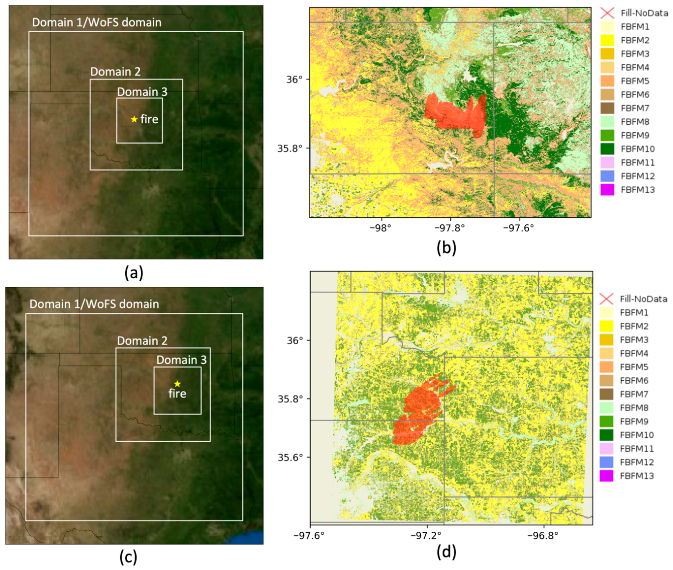
In this study, SFIRE is configured with three one-way nested domains containing 60 vertical levels up to 20 hPa. A linkage between WoFS-Smoke and SFIRE is introduced, where the WoFS-Smoke domain serves as the outermost domain of SFIRE to enable qualitative and quantitative verification between the two models. Consequently, the outermost domain covers approximately 900 × 900 km with a 3 km horizontal grid spacing (
Figure 1a,c). The horizontal grid spacings of the inner nests are 1 km and 500 m, respectively. An additional fire domain was embedded in domain 3 with a resolution of 50 m, one-tenth of the atmosphere domain 3, for fire spread modeling (
Table 1). The 2023 LANDFIRE data (
https://landfire.gov/, accessed on 15 May 2025) that classifies fuel characteristics to Anderson 13 fuel models [
53] at 30 m resolution are used for all the case studies in this work because they are the most recent updated fuel maps prior to both of the case studies (
Figure 1b,d). The elevation data are sourced from the LANDFIRE 2020 update elevation product with the same grid size as the fuel maps.
The emission models used to define “smoke” in WoFS-Smoke and SFIRE are very different and have been tuned for their expected applications. For example, smoke emissions are defined primarily on satellite-retrieved FRP coupled with land surface coverage. In SFIRE, emissions are calculated from the amount of fuel being burned, in addition to other parameters. WoFS-Smoke also has an internal maximum smoke concentration threshold of 5000 μg kg−1, which is reached in strong wildfires. As a result, smoke emissions from SFIRE are generally much larger than the WoFS-Smoke counterpart. For these experiments, smoke is considered to be an inert tracer, and no chemical interactions are included. Two sets of forecasts are compared with one originating from classic WoFS-Smoke using a single domain and no coupling. The second uses WoFS-Smoke as an initial condition for an SFIRE simulation of wildfires. Two forecast initialization times were selected for each event, separated by one-hour intervals, and two sets of forecasts were generated. One using classic WoFS-Smoke and another using classic WoFS-Smoke analyses as initial conditions for an ensemble of SFIRE forecasts.
A 5 min spin-up period was applied, during which the WRF atmospheric model was run without fire to allow the innermost domain to develop a well-mixed boundary layer. Following the WoFS-Smoke approach, an 18-member ensemble was used. Initial heat fluxes were derived from FRP values used by that member in classic WoFS-Smoke, assuming a conversion factor of approximately ten, as used by [
49,
54].
3. Results
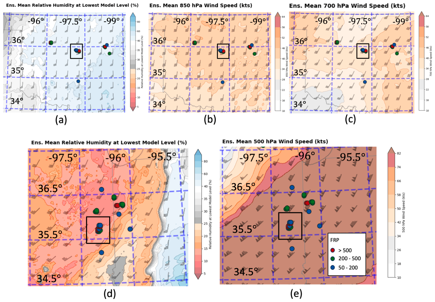
The smoke forecasts from WoFS-Smoke and WRF-SFIRE, initialized using WoFS, were compared across two case studies that were selected based on the availability of model initial conditions and observations. The first case study focuses on the Cimarron Bend Fire in central Oklahoma that started on 29 October 2024. The fire was reported at 2003 UTC (3:03 PM Central Daylight Time [CDT]) 4 miles northwest of Cashion, Oklahoma, and was detected from GOES-16 data around 1930 UTC at 35.87° N, 97.84° W. The relative humidity (
Figure 2a) around the fire site was 40–50% with 20 kts (10 m s
−1) surface winds from the south. Flow from the southwest is present between the 850 hPa (
Figure 2b) and 700 hPa (
Figure 2c) levels with wind speed on the order of 40 kts (20 m s
−1) over the fire.
The second case study focuses on one of a series of wildfires that occurred in central Oklahoma on 14 March 2025. The dynamics at the fire site of interest are illustrated in
Figure 2d,e. Extreme fire weather conditions near the site favored wildfire ignition and rapid growth. At 1900 UTC (2:00 PM CDT), relative humidity dropped below 10%, and temperatures reached approximately 70 °F (21 °C). A continuous wind field extended from the surface up to 500 hPa, with strong southwesterly flow. Surface wind speeds reached 35 kts (18 m s
−1), while winds at 500 hPa exceeded 80 kts (41 m s
−1).
As shown in
Figure 1b, the majority of the 2024 Oklahoma fire site was characterized by closed, short-needle timber litter (FBFM8) and hardwood or long-needle pine timber litter (FBFM9), with a smaller portion of mature/overmature timber and understory (FBFM10) located on the northeastern edge. The fire propagated northward, driven by surface winds from the south. A higher rate of fire spread was observed on the northeastern side of the fire area, likely due to the presence of more flammable fuels (FBFM9 and FBFM10). For the fire on 14 March 2025, the behavior fuel model at the site consists of a mixture of grass (FBFM2) and hardwood/timber litter (FBFM9). Driven by strong southwesterly winds, the fire spread northeastward, exhibiting a relatively uniform rate of spread across the affected area.
Comparisons between WoFS-Smoke and SFIRE are facilitated by using Multi-Radar/Multi-Sensor (MRMS) reflectivity observations as a benchmark. Radar data can provide information on 3D plume characteristics at a high temporal resolution (<5 min) by detecting debris lofted alongside smoke aerosols. Since debris particles are larger and heavier than aerosols, these radar observations serve as a lower bound for the expected smoke distribution and maximum plume height [
55,
56].
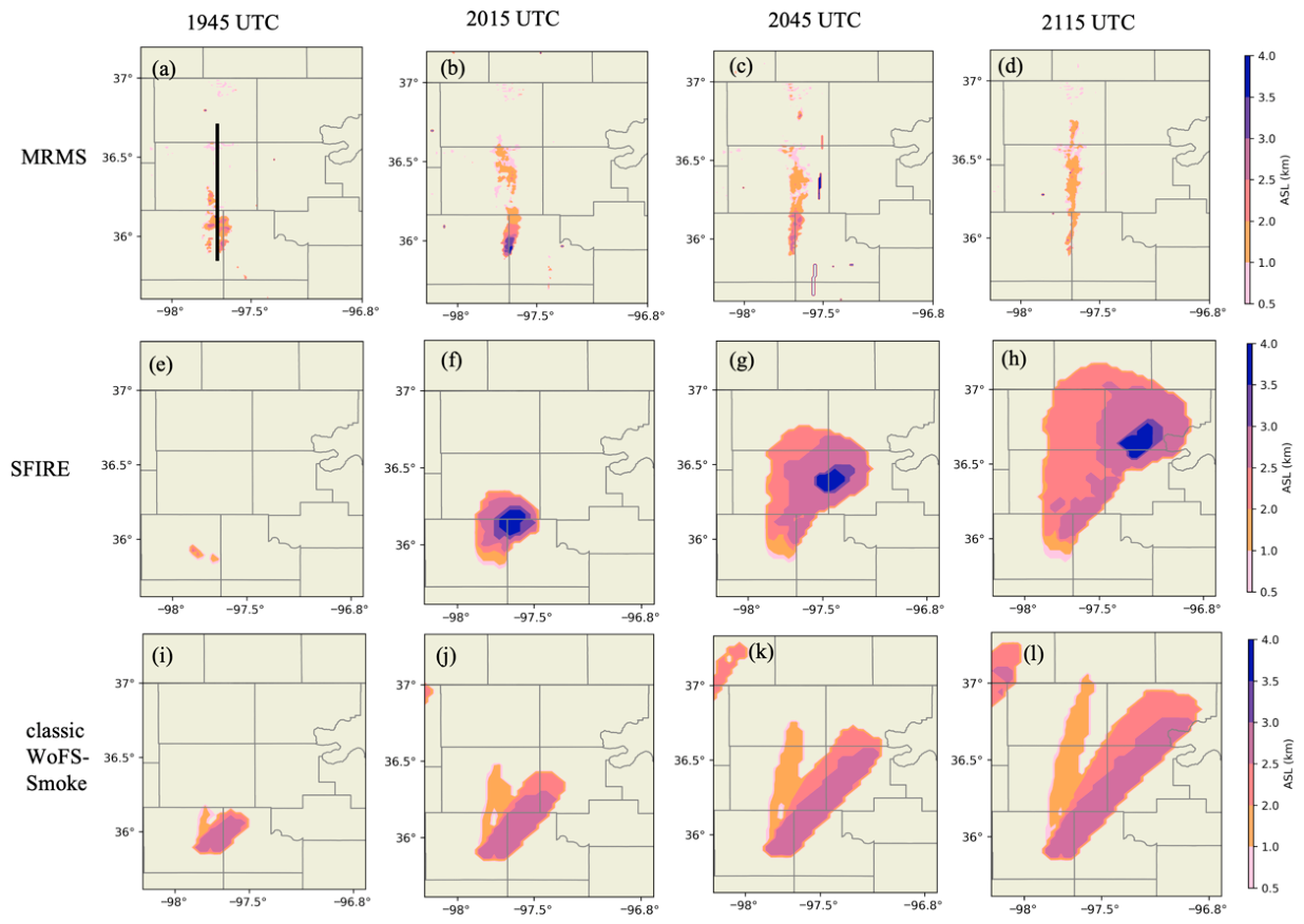
To evaluate the ability of SFIRE and classic WoFS-Smoke to resolve the vertical distribution and extent of smoke plumes, we compared the simulated plume-top heights with MRMS reflectivity over a 1.5 h forecast period (1945–2115 UTC), as shown in
Figure 3. Plume heights are defined as the model level where forecast smoke decreases below 1 mg kg
−1. For radar data, a threshold of 5 dBZ is used. Both estimates contain some uncertainty and are provided to assess large-scale (>1 km) differences. Radar data at 1945 UTC indicates two smoke plumes dispersing northward (
Figure 3a). The western plume weakened by 2015 UTC owing to a decrease in intensity of its host fire, while the eastern plume dominated the smoke dispersion and persisted through 2115 UTC. The estimated plume height from radar data was less than 3 km ASL throughout this period.
Both the SFIRE (
Figure 3e–h) and the classic WoFS-Smoke forecasts (
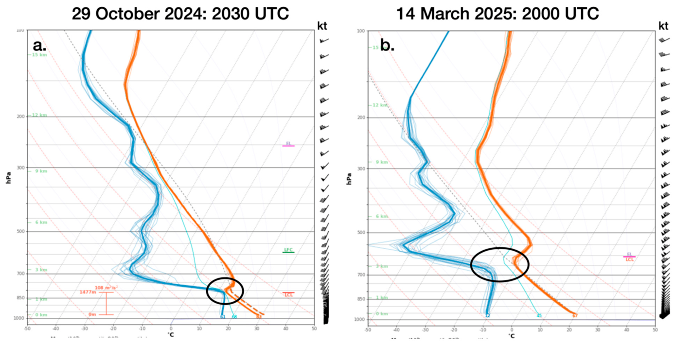
Figure 3i–l) indicate a northward extension of low-level smoke (plume height below 2 km ASL). However, both also forecast smoke plumes that propagate in a more northeasterly direction compared to the due north propagation observed from radar data. This is a result of overestimated plume height, which led to the injection of smoke aerosols above the boundary layer, where winds changed from a southerly to a southwesterly direction. Planetary boundary layer height was estimated to be ~2 km ASL based on a simulated model sounding near the wildfire at 2000 UTC (
Figure 4a).
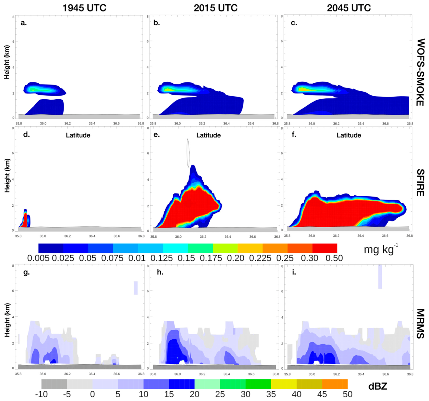
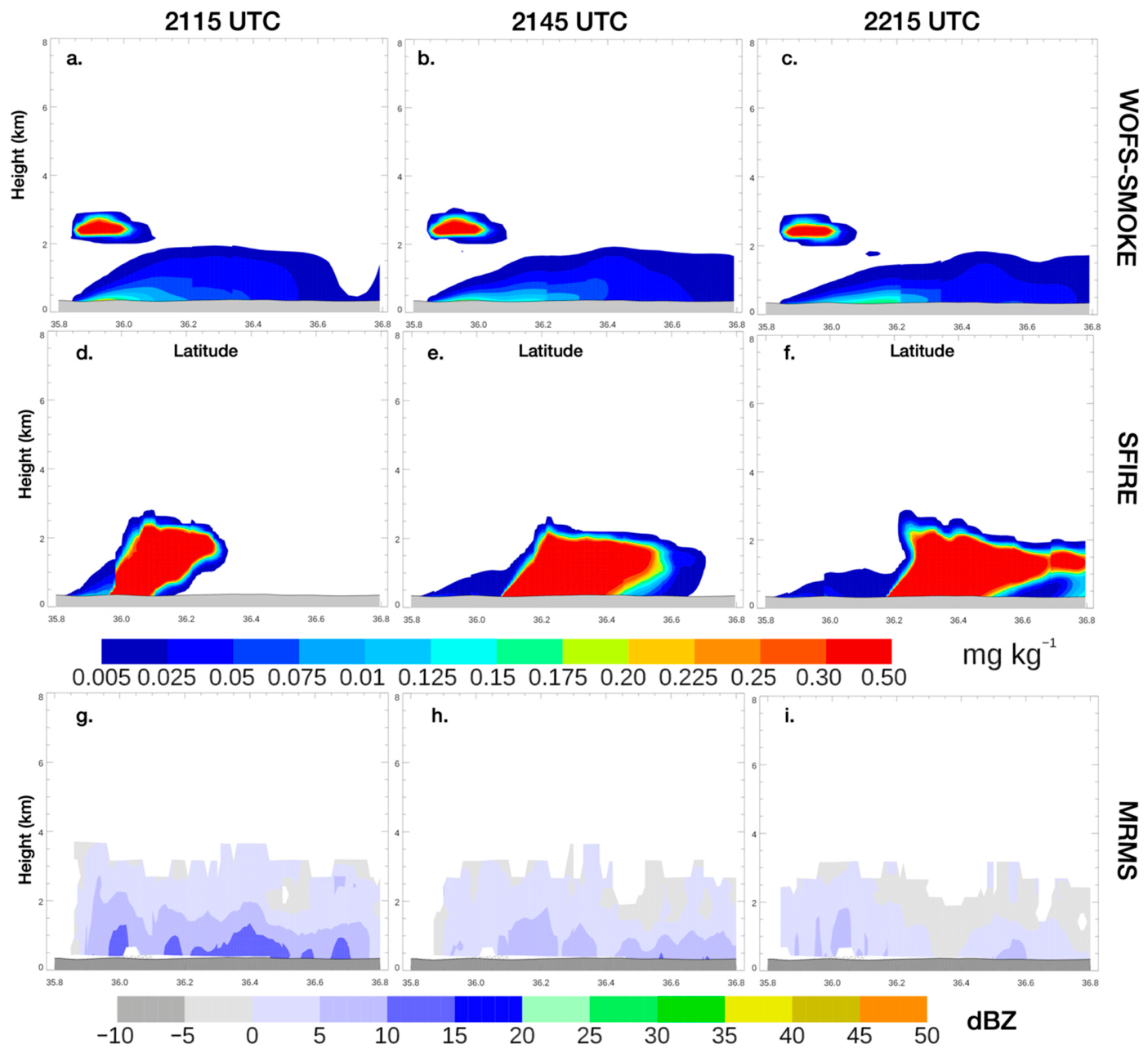
The impact of smoke height and the environment is clearest in classic WoFS-Smoke, with one forecast plume whose height is <2 km ASL being transported northward, consistent with the data. The direction of dispersion gradually shifted from northward to northeastward as forecast smoke lofted above the boundary layer was driven by the mid-level flow. The vertical structure of smoke can be further evaluated using the cross-section shown in
Figure 5, corresponding to the black line marked in
Figure 3a. MRMS reflectivity indicates that smoke and biomass burning debris were concentrated between 1 and 2 km ASL, with most particles remaining below the boundary layer. Classic WoFS-Smoke emissions occur near the surface and aloft, where the injection height is estimated. Note that the plumes near the surface and the one near the injection height are not linked and are mostly independent of each other (
Figure 5a–c). If the upper plume were simply eliminated from the forecasts, smoke emission characteristics in classic WoFS-Smoke would be much more realistic. This dual-plume characteristic in the smoke forecast is not physically realistic, showing the limitations of this system.
Figure 5a–f illustrates the vertical smoke distribution forecasted by classic WoFS and SFIRE experiments. In SFIRE, smoke tracers originate directly from the fire source, where the smoke concentration is highest, and are transported upwards from the thermodynamic-induced buoyancy. Smoke particles are lofted up to ~3 km ASL, similar to the heights forecasted in classic WoFS-Smoke (
Figure 3). However, this vertical profile exhibits high continuity, resulting in much more realistic smoke distribution despite also being an overestimate. Forecast smoke concentrations are also significantly greater at later forecast times in SFIRE, but it is important to note that “smoke” aerosol definitions are not fully consistent between the two systems. Radar data along this path indicate a relatively shallow debris plume that varies in intensity downstream owing to changes in debris injection from variability in wildfire intensity (
Figure 5g–i).
A second forecast set, initiated one hour later at 2030 UTC, was generated at the same fire site to assess the difference between systems once the wildfire has become more established. Plume height characteristics were very similar, but larger differences in the vertical profile and amounts of smoke being injected are evident. Profiles of ensemble mean smoke forecasts along the same path as those in
Figure 3 show that classic WoFS-Smoke forecasts much larger smoke emissions than previously, but the dual plume structure remains (
Figure 6). In WoFS-Smoke, emissions are effectively carried over from one forecast cycle to the next, leading to an increase in smoke concentrations assuming a constant FRP. Recall that SFIRE resets emissions once initiated, so smoke from the previous cycle is not taken into account in this configuration. The wildfire location in classic WoFS-Smoke is also unchanged since fire spread over the forecast period is not taken into account. In the case of the SFIRE run, the spread of the fire northward is clearly evident with the smoke plume core moving from 36.05° at 2115 UTC to 36.25° by 2215 UTC. As with the previous forecast set, the vertical structure of smoke in SFIRE is much more realistic, but maximum smoke heights are again overestimated. Radar data at these times show that lofted debris concentrations have lowered significantly since 2100 UTC, indicating that the wildfire was decreasing in intensity.
These results suggest that both models perform poorly during the fire-diminishing stage. In addition to the limitations of static FRP injections, assumptions about fuel consumption further constrain model performance. In the SFIRE configuration used here, we assume 100% fuel consumption, which leads to overestimation during the smoldering phase. This was the default setting, but further sensitivity testing of this parameter is likely warranted.
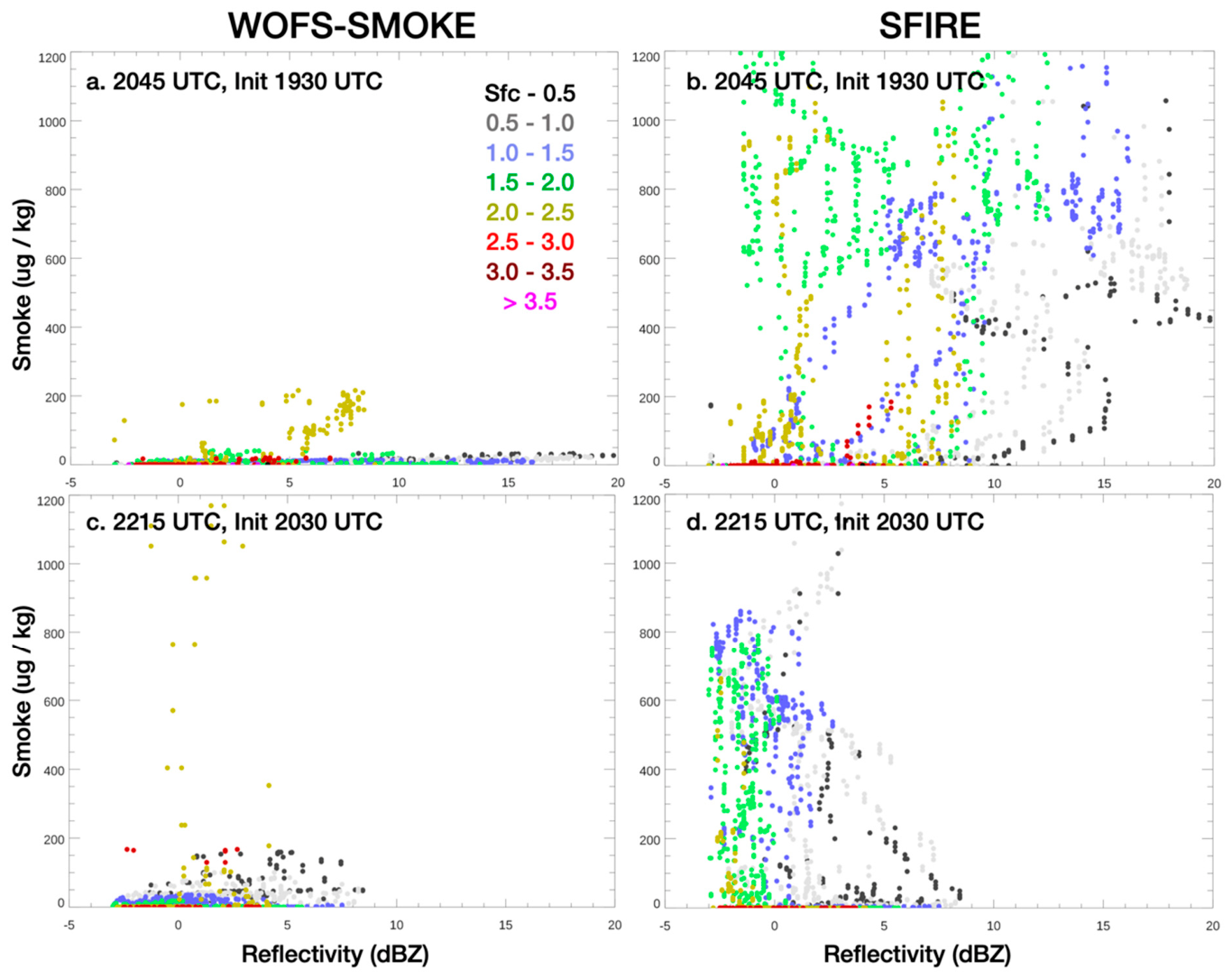
Another way of visualizing these differences is to compare 3-D MRMS reflectivity and ensemble mean forecast smoke at each grid point along the cross sections shown in
Figure 5 and
Figure 6. To create these comparisons, MRMS reflectivity is resampled to the WoFS grid, and scatter plots of reflectivity vs. smoke are generated for data along the given cross-section.
Figure 7 shows this comparison for classic WoFS-Smoke (a) and SFIRE (b) for a 75 min forecast initiated at 1930 UTC. Clear differences between the experiments are readily apparent, with classic WoFS-Smoke forecasting very small smoke concentrations even where corresponding reflectivity exceeds 10 dBZ. Only for data in the 2–2.5 km layer are smoke concentrations >50 μg kg
−1 present. Importantly, no smoke emissions are forecast where the highest reflectivity was observed. A similar comparison for SFIRE shows strikingly different results (
Figure 7b). Much higher smoke emissions are present and exist in the entire column from near the surface up to approximately 2.5 km. Highest reflectivity observations generally correspond with smoke in the lowest 1 km, which is consistent with the cross-sections above. Furthermore, higher-altitude smoke generally corresponds to lower reflectivity values. At a later forecast time (105 min from 2030 UTC), similar patterns are evident, though some key differences exist (
Figure 7c,d). In classic WoFS, the greatest smoke emissions are still forecast in the 2–2.5 km layer, but near-surface smoke is also now present. Note that lofted debris has decreased significantly from 2045 UTC, with maximum reflectivity being <9 dBZ along this cross-section. SFIRE also forecasts smoke decreasing compared to 2045 UTC, but low-level smoke still corresponds to higher reflectivity values, and more lofted smoke corresponds to lower reflectivity. In particular, smoke emissions near 2 km only correspond to reflectivity observations less than 0 dBZ. While the difference in height and total emission characteristics is clear, the correlation between smoke and reflectivity on a grid-point to grid-point scale is generally low. Given the differences in the particles being modeled and those that are being observed, low overall correlations are not surprising.
- b.
Oklahoma, 14 March 2025
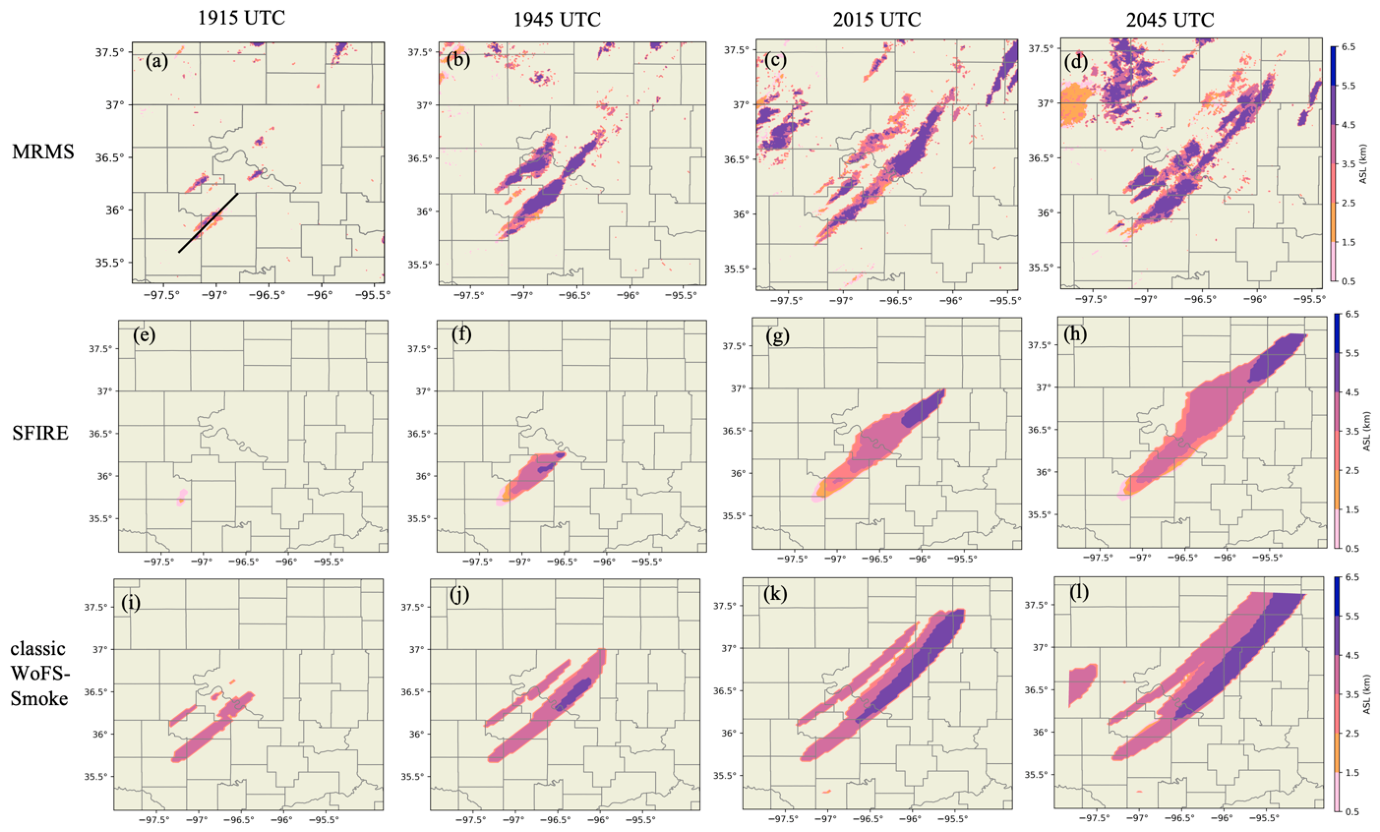
A second case study focuses on the 14 March 2025 Oklahoma wildfire outbreak, and two sets of forecast experiments were generated with initialization times at 1900 UTC and 2000 UTC, respectively. For the 1900 UTC initialization, forecasted plume-top heights were compared with radar reflectivity over a 1.5 h forecast period (1915 UTC–2045 UTC) as shown in
Figure 8. Multiple debris plumes are evident in the radar data, which increase in size substantially after 1930 UTC. Debris plume heights reach ~5 km ASL over large areas for several fires.
For this case, we focus on the southwestern-most fire, which generated the largest smoke plume during this period. SFIRE is initialized with the location and intensity associated with this fire and does not simulate the others in the domain. Thus, the SFIRE smoke forecasts shown here do not include emissions from the other fires that are present in observations and in classic WoFS-Smoke. Both systems forecast the primary smoke plume well, with similar size and height characteristics to the radar-derived debris plume heights. However, the finer-scale features in the radar data are smoothed out in the model forecasts.
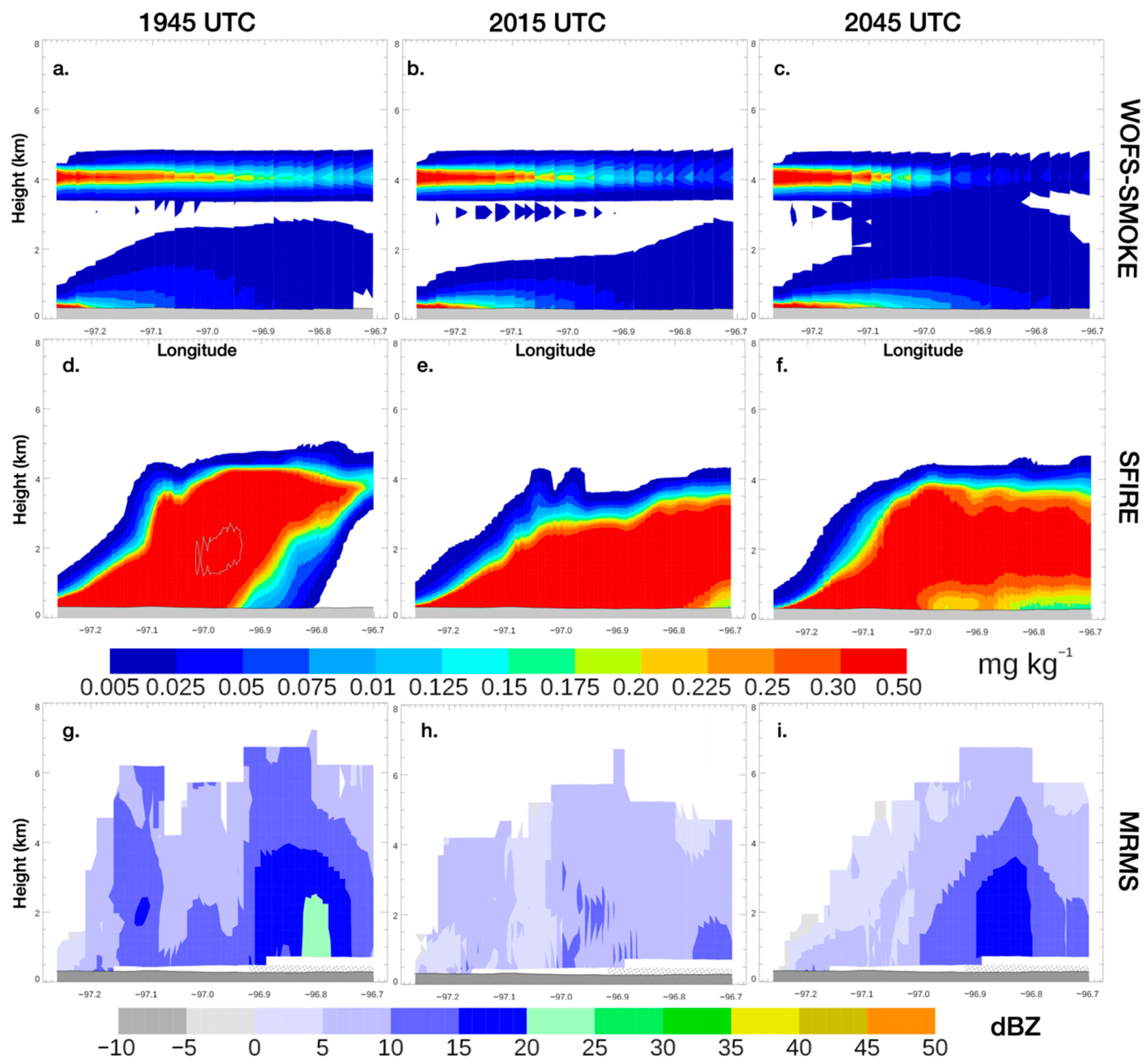
In the SFIRE experiment, it takes ~1 h to fully spin up and transport smoke a similar distance downstream compared to observations and classic WoFS forecast smoke plumes. By 2015 UTC, differences in the plume height characteristics between the two experiments became more apparent. SFIRE forecasts plume heights ~ 2 km ASL near the origin, which gradually increase to >5 km ASL further downstream. Classic WoFS forecasts smoke at higher levels throughout most of the plume’s length. Debris plume heights from radar data seem to agree with the higher estimate, but there is also a high degree of variability in the observed plume heights in both space and time. To further examine the vertical distribution of smoke and debris, a cross-sectional analysis was performed along the cross-section marked by the black line in
Figure 8a, with results shown in
Figure 9 and
Figure 10.
Vertical smoke distribution was compared between 1945 UTC and 2045 UTC to allow sufficient spin-up time for SFIRE to develop a well-structured plume. While SFIRE generally underestimated plume height, it generated a much more realistic distribution of smoke compared to classic WoFS. The former retains the dual plume structure found in the previous case, with smoke injection occurring near the surface and at the estimated injection height of ~ 4 km ASL. WoFS-analyzed soundings near the wildfire location also indicate the boundary layer near this level, along with very strong southwesterly winds reaching up to 100 kt near this layer (
Figure 9b). As before, there is no analyzed connection between the lower and upper smoke plumes despite very dynamic atmospheric conditions. Radar data indicates smoke and debris throughout this level, with height and concentrations increasing further downstream of the origin.
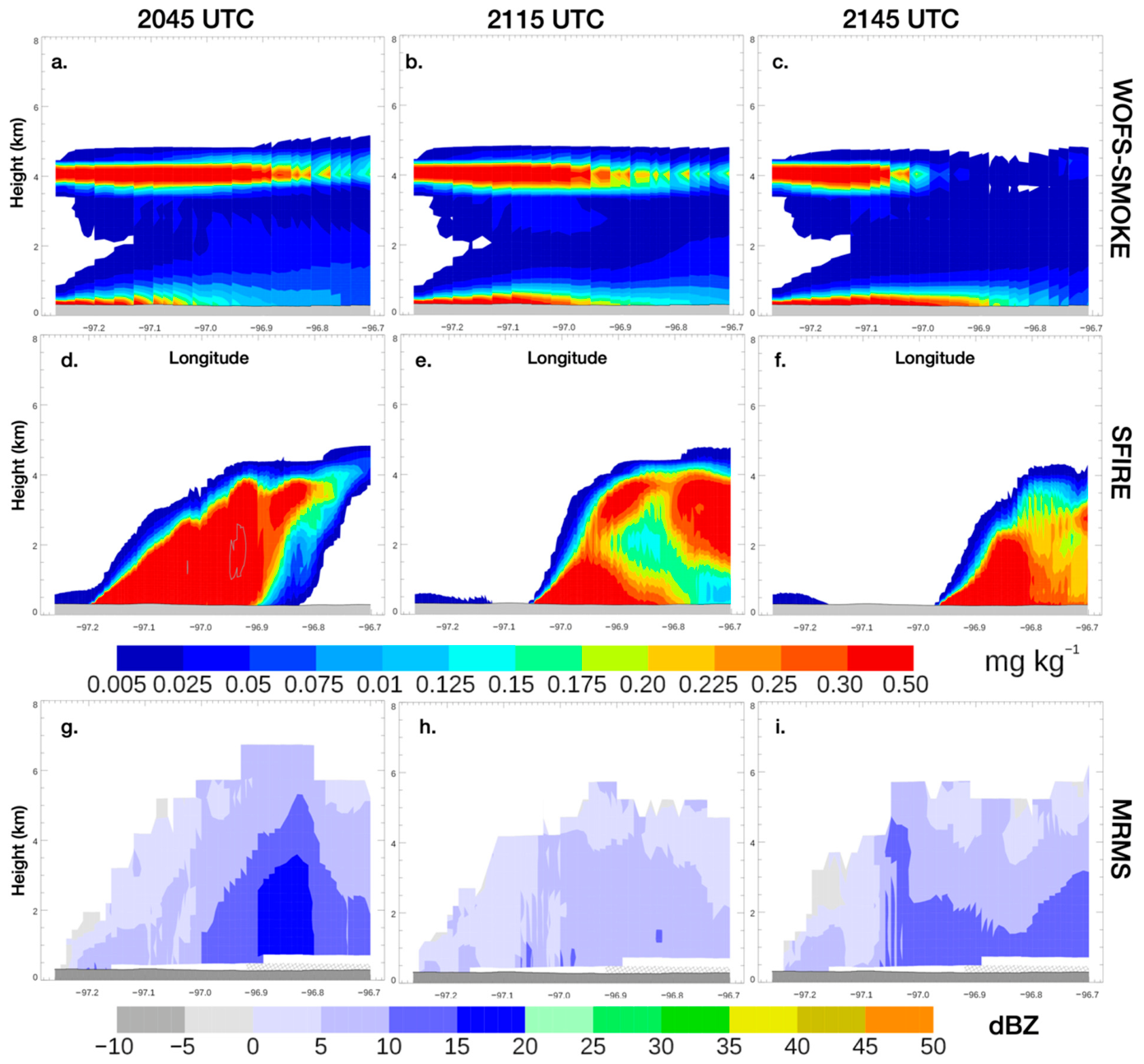
A second set of smoke forecasts, shown in
Figure 10, covers 2045–2145 UTC from forecasts initiated at 2000 UTC. Cross-sections along the same paths were generated for comparison of the two experiments with radar data. The fire front in SFIRE advances from 97.1° W (
Figure 10d) to 97.0° W (
Figure 10e) from 2045 to 2115, in good agreement with MRMS-detected reflectivity (
Figure 10g,h). SFIRE’s simulated plume height and vertical smoke structure are also consistent with the radar observations. However, by 2145 UTC, the simulated fire propagated farther east than indicated by MRMS reflectivity (
Figure 10f,i), indicating that the modeled fire spread was too rapid. This could be due to a multitude of factors, including the initial fire intensity and perimeter being too large, and near-surface winds being overforecast. Still, SFIRE’s ability to simulate the downstream evolution of the fire front represents a significant advantage over the classic system.
Classic WoFS-Smoke predicts high condensations of smoke in the 4–5 km ASL layer, while most surface smoke remains below 1 km ASL. The dual plume feature is being retained, though some smoke is now present between these layers. Furthermore, the WoFS-Smoke forecast does not capture the plume progression observed in the radar data, leading to potential overestimation of smoke emissions in burned-out areas.
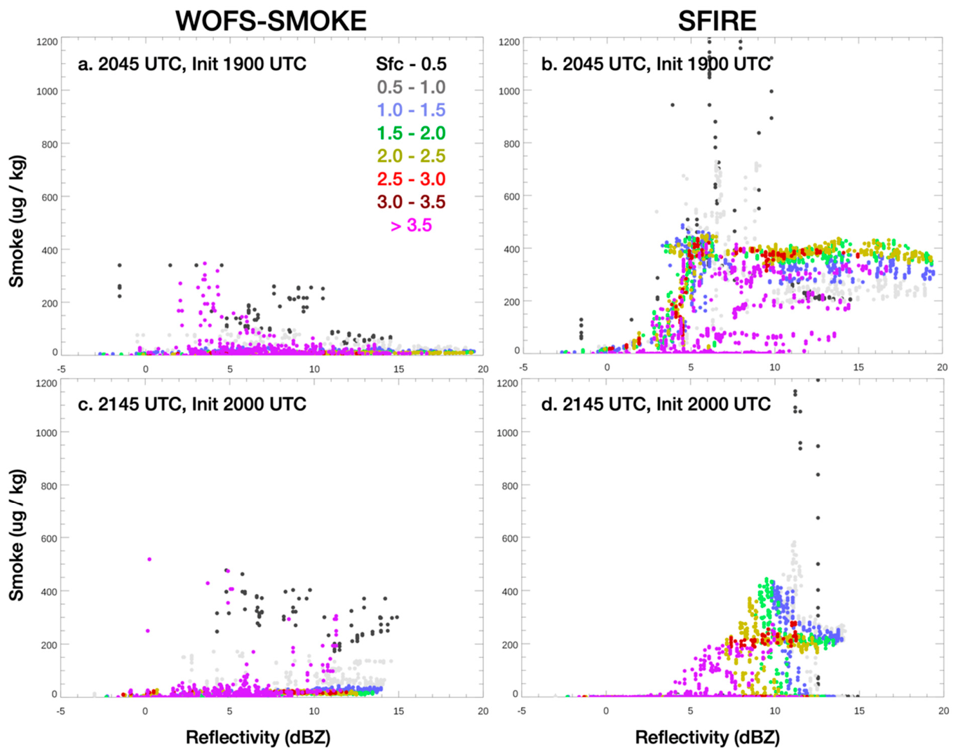
Scatter plots of forecast 3-D ensemble mean smoke and reflectivity across these cross-sections show that forecast smoke concentrations from classic WoFS are often very small even where observed reflectivity is >10 dBZ (
Figure 11a,c). Where smoke does exist, it is generally located below 1 km or in the 3–4 km layer. SFIRE forecasts are much different, with smoke concentrations >200 μg kg
−1 associated with reflectivity > 5 dBZ from near the surface up to over 3.5 km for the 2045 UTC forecast initiated at 1900 UTC (
Figure 11b). The highest smoke concentrations lie near the surface with values >400 μg kg
−1, though these do not correspond to maximum reflectivity observations. Above the surface layer, the scatter plot pattern suggests that where reflectivity exceeds 10 dBZ, smoke concentrations generally increase as a function of height. This indicates that where the radar debris signature is greatest, buoyant updrafts are also lofting large amounts of smoke upward, which SIFRE seems to correctly simulate. At later times, the intensity of the smoke and debris plume decreased somewhat, with observed reflectivity generally less than 15 dBZ at 2145 UTC (
Figure 11d). At this time, the smoke distribution is similar to that observed in the October case, with the highest reflectivity corresponding to the lowest-level smoke with lower values at higher levels.
4. Discussion and Conclusions
This study employed WRF-SFIRE simulations driven by inputs from classic WoFS analyses and compared the resulting forecasts with those from classic WoFS-Smoke. Both systems demonstrate comparable agreement with observations, though each possesses distinct advantages and limitations. SFIRE typically requires a 30 min to one-hour spin-up period to generate sufficient particles and establish a well-structured plume in this configuration. Beyond this period, SFIRE often outperforms WoFS-Smoke due to its fire–atmosphere coupling, which more accurately represents physical fire processes. In contrast, the classic WoFS-Smoke model directly inserts particles at injection heights determined by the Freitas model. This approach produces unrealistic bi-model vertical distributions in these examples.
Classic WoFS-Smoke forecasts initialize using smoke fields from previous cycles, enabling them to provide guidance immediately (i.e., within 5 min). However, this reliance on accumulated smoke limits the model’s sensitivity to reductions in fire intensity, increasing the risk of overestimation during periods of inactivity. Conversely, SFIRE starts from a clear field; while this allows for greater sensitivity to changes in fire intensity, the resulting need for spin-up time restricts its utility for real-time forecasting. Despite the generally superior performance of SFIRE due to fire–atmosphere coupling, its computational demands are substantial, with runtimes up to three times longer than those of classic WoFS-Smoke.
Sub-hourly smoke forecasts are critical because smoke plumes often evolve rapidly due to shifting winds and sudden bursts of fire intensity, rendering standard hourly updates insufficient for immediate situational awareness. The high-frequency guidance enables emergency managers to respond to acute hazards in real-time, such as issuing timely warnings for dangerous reductions in visibility on roadways and protecting aviation and ground crews during suppression operations. This study highlights the potential of SFIRE for sub-hourly forecasting, as well as its distinct advantages and disadvantages compared to classic WoFS-Smoke. Although both models are capable of producing acceptable agreement with observations, common limitations restrict their performance under certain conditions. Both models exhibit a tendency to underestimate plume height under strong inflow conditions, necessitating further adjustment based on radar observations in operational settings. However, the spin-up lag associated with the SFIRE runs can be eliminated if fires are initiated and updated in the system when they are initiated and not after they have already matured. We also recognize that a testing sample comprising only two Oklahoma fires may not provide results that apply to different wildfire conditions with different geographic, soil, and vegetation characteristics. Further work testing a more diverse set of wildfire events is planned.
Future work should aim to mitigate these limitations by integrating more comprehensive physical processes and advanced observational data. Specifically, incorporating explicit dry and wet deposition schemes, alongside the assimilation of high-frequency satellite FRP data, would significantly improve model sensitivity to decaying fire activity and reduce overestimation errors. Furthermore, the tendency to underestimate plume heights under strong inflow could be addressed by refining entrainment parameterizations in plume rise models or by directly assimilating 3D radar reflectivity to constrain the vertical smoke distribution. Finally, developing hybrid initialization strategies that combine the rapid ‘warm start’ capability of WoFS with the physically coupled environment of SFIRE could minimize spin-up latency, thereby enhancing the operational feasibility of high-fidelity, sub-hourly forecasts.