MFFLNet: Multi-Scale Fire Feature Learning for Fire Video Recognition

Abstract

Accurate and timely recognition of flame and smoke is critical for fire warning systems to mitigate casualties and property damage. Most existing fire datasets are image-based and thus fail to capture the dynamic spatiotemporal information of fire. Furthermore, the lack of large-scale fire video datasets poses a significant challenge to the training of neural networks. To address these limitations, we developed the Flame-Smoke Video Recognition (FSVR) dataset, a large-scale collection of 30,000 video clips that significantly exceeds the scale of prior datasets in the same domain. Since flame and smoke exhibit multiscale characteristics, small-scale targets are often obscured by complex backgrounds. Existing methods lack robust multiscale feature learning capabilities, which limits their ability to achieve precise fire recognition under complex conditions. To address this issue, we proposed the Multi-scale Fire Feature Learning Network (MFFLNet), which integrates multiple Multi-scale Fire Feature Learning (MFFL) blocks into a Transformer backbone. Each MFFL block comprises two key components, i.e., the multiscale fire Conv3D layer and the fire spatiotemporal feature learning layer. The experimental results obtained from the FSVR and LFVR datasets demonstrate that MFFLNet surpasses the baseline model and other comparative methods. When the backbone network is initialized with pre-trained weights from the Kinetics-710 dataset, MFFLNet attained an accuracy of 79.54% and a macro-F1 score of 79.22% on the FSVR dataset, while achieving an accuracy of 95.64% and an F1 score of 95.46% on the LFVR dataset.

1. Introduction

Fire incidents lead to loss of life and property globally [1,2]. Vision-based fire warning has emerged as a significant research direction [3,4]. Sensors and cross-technology communication are also research directions [5,6,7]. Existing public fire datasets are predominantly image-based. Consequently, they lack the dynamic spatiotemporal characteristics of flame and smoke. This scarcity of video data hinders the training of networks. Consequently, the construction of a large-scale, high-quality fire video dataset is of substantial research significance.

The multiscale characteristic of flame and smoke in real-world scenarios presents significant challenges for fire recognition. While large flame and smoke are relatively easy to identify, small ones are often concealed in complex backgrounds and exhibit a similarity to the background textures and colors, thus posing challenges for fire recognition. However, most previous methods lack the ability to effectively learn the multiscale features of fire. Enhancing the model’s ability to accurately recognize multiscale flame and smoke remains a challenge in the field of Fire Video Recognition (FVR).

To address the scarcity of public fire video datasets, we constructed the large-scale Flame-Smoke Video Recognition (FSVR) dataset. This dataset encompasses diverse real-world fire scenarios, and provides ample training data for deep learning models. To overcome the limitations in multiscale feature learning, we proposed the Multi-scale Fire Feature Learning Network (MFFLNet), which integrates multiple Multi-scale Fire Feature Learning (MFFL) blocks within a Vision Transformer (ViT) [8] backbone. This design effectively enhances the learning of multiscale fire features and improves the recognition accuracy of flame and smoke. Each MFFL block comprises two key components: a Multi-scale Fire Conv3D (MFConv3D) layer and a Fire Spatio-Temporal Feature Learning (FSTFL) layer. By leveraging multiple 3D convolutions with varying kernel sizes and a maximum fusion operation, MFConv3D fuses fire features across different scales. Through operations including 3D convolution, average pooling, and channel compression, FSTFL learns the spatiotemporal features of fire. Experimental results demonstrate that MFFLNet outperforms the baseline and other methods on both the FSVR and LFVR [9] datasets. The main contributions are as follows.

• We constructed the FSVR dataset, comprising 30,000 clips across diverse real-world scenarios. This dataset provides substantial data support for FVR, which is conducive to advancing research in this domain.
• MFFL was proposed, which is composed of MFConv3D and FSTFL. By innovatively integrating the 3D convolution, average pooling, channel compression and maximum fusion, it enhances the multiscale fire feature learning capability of the neural network.
• MFFLNet was designed, which integrates the MFFL blocks within a ViT backbone. By learning the multiscale features of fire, MFFLNet attains state-of-the-art performance on two public datasets.

2. Related Work

Notable advancements have been achieved in the development of fire recognition datasets and fire-warning systems [10]. This section focuses primarily on research related to fire recognition datasets and fire recognition methods.

2.1. Fire Recognition Datasets

The construction of high-quality datasets is essential for advancing the fire warning system [11]. Fire incidents in real-world scenarios are diverse, making it challenging to comprehensively represent them using a single data source. Consequently, recently released public fire recognition datasets have provided robust support for algorithm training and validation.

Table 1. Fire recognition datasets.

Dataset	Category	Year	Type	Number
Corsican fire [12]	Fire	2017	Image/video	600/5
FiSmo [13]	Fire and smoke	2017	Image/video	9448/88
FireNet [14]	Fire	2019	Image/video	2585/62
DSDF [15]	Smoke	2020	Image	18,413
D-Fire [16]	Fire and smoke	2021	Image/video	21,527/100
Nemo [17]	Smoke	2022	Image/video	4347/95
DFS [18]	Fire and smoke	2023	Image	9462
LFVR [9]	Fire	2024	Video	11,560
MS-FSDB [19]	Fire and smoke	2024	Image	12,586
FSVR	Fire and smoke	2026	Video	30,000

presents several datasets in this field.

Flame-only datasets focus on identifying visible flame across various scenarios, including building and forest fires. These datasets often include interference objects, such as sunsets and red-colored items. The Corsican Fire dataset [12] is specifically tailored for wildfire monitoring and comprises 500 wildfire images, 100 near-infrared images, and 5 videos. The training set of FireNet [14] comprises 1124 flame-inclusive images and 1301 non-flame images, whereas the test set consists of 46 flame-inclusive videos, 16 non-flame videos, and 160 non-flame images. LFVR [9] contains 11,560 video clips sourced from the internet and real-world recordings, covering different scales, scenarios, and burning objects, thus exhibiting high diversity. A significant limitation of these datasets is their reliance on flame, which precludes early fire warning.

Smoke-only datasets are designed to facilitate early fire warning. These datasets include smoke at varying concentrations and use visually similar entities as primary interference. The DSDF dataset [15] is specifically designed for smoke recognition, containing 18,413 images. Nemo [17] is a dataset designed for fine-grained fire and smoke recognition, comprising 4347 images and 95 test videos. Smoke-only datasets have theoretical advantages in early fire warning. However, methods that solely rely on smoke detection are associated with relatively high false-alarm rates.

To address the aforementioned issue, researchers have constructed datasets for fire and smoke recognition. These datasets are compiled from diverse sources, such as surveillance videos, drone images, satellite images, etc. The FiSmo dataset [13] comprises an image sublibrary and a video sublibrary, totaling 9448 images and 88 videos. The D-Fire [16] dataset contains 21,527 bounding-box-annotated RGB images and 100 test videos. The DFS [18] dataset subdivides 9462 images by fire intensity into three categories. MS-FSDB [19] contains 12,586 images, including 3603 positive and 8983 negative samples.

2.2. Fire Recognition Methods Based on Handcrafted Features

Color features, as the most intuitive visual representation of flame, were central to early fire recognition methods. By exploring the representation capabilities of various color spaces, researchers achieved localization and classification of flame. For instance, Foggia et al. [20] implemented video flame detection by designing a system that integrates the color distribution, dynamic shape variations, and motion trajectory characteristics of flame.

The detailed analysis of motion features has become a significant research direction. Torabian et al. [21] proposed a motion analysis-based method that distinguishes flame from other moving targets by capturing their motion patterns. To improve the performance in dynamic scenes, Dou et al. [22] focused on the features of motion and color of flame. For fire image classification, Harkat et al. [23] employed machine learning techniques to compute higher-order features. For forest fire detection, Zhang et al. [24] proposed a vector machine.

The multi-modal data fusion technology has enhanced the accuracy of fire recognition. To improve fire detection performance, Sharma et al. [25] fused sensor data with environmental data and aggregated model parameters through a federated learning framework. By utilizing multispectral data, Mfondoum [26] proposed a multi-filter active fire mapping method. Panneerselvam et al. [27] proposed a fire recognition method based on federated learning. Liu et al. [28] proposed a fire classification framework that integrates aspect ratio quantitative analysis and point cloud segmentation.

2.3. Fire Recognition Methods Based on Deep Learning

Deep learning-based fire recognition methods have evolved from single-image classification to comprehensive spatiotemporal frameworks. To meet the requirements of diverse scenarios, extensive research has been conducted on model architecture, multimodal fusion, etc.

Regarding architectural innovation, various advanced architectures have been applied to address the diversity and complexity of fire scenarios. Lightweight design is essential for meeting real-time recognition requirements. Muhammad et al. [29] adopted the lightweight MobileNetV2 network to adapt to computational demands in uncertain environments. YOLO-LFD [30] employs depthwise separable convolutions to reduce computational complexity. To enhance the perception of fire, Shahid et al. [31] integrated attention mechanisms into a convolutional neural network. Similarly, CCi-YOLOv8n [32] optimizes the detection of small-fire targets by integrating CARAFE and context-guided blocks. MTL-FFDET [33] is a fire recognition method based on multi-task learning. Bendouma et al. [34] proposed a two-stage method to address complex background interference. Majid et al. [35] leveraged transfer learning and attention mechanism to enhance the generalization ability. LGAE [9] enhances performance by designing the LAME and GAME blocks to effectively capture local and global motion characteristics of fire.

To overcome the limitations of single-source visual data, researchers have focused on integrating multimodal information. Sheng et al. [36] proposed a method enhanced by SLIC-DBSCAN, utilizing clustering algorithms to pre-identify suspected fire and smoke regions. For wildfire monitoring, Dong et al. [37] developed a framework to predict the spatiotemporal dynamic of fire. Han et al. [38] designed a Transformer-based method that addresses image resolution degradation in forest fire. For fire recognition in industrial environments, Deshpande et al. [39] designed a system utilizing transfer learning that operates stably under low visibility and adverse weather conditions.

In contrast to these methods, MFFLNet is a multiscale feature learning approach for FVR. Through the MFFL block, MFFLNet captures feature information of flame and smoke at different scales and enhances key features, thereby improving the recognition capability for fire.

2.4. Methods Based on Multi-Scale or Attention Mechanisms

Spatiotemporal feature modeling methods for videos can be broadly classified into two categories: multi-scale convolution-based approaches and attention-based approaches. While both categories have yielded notable achievements, they exhibit inherent limitations when applied to the FVR task.

Multi-scale 3D Convolution (M3D) [40] captures spatiotemporal information across varying receptive field scales. Building upon 2D convolutions, M3D utilizes multiple parallel temporal convolutional kernels with different dilation rates to achieve multi-scale feature extraction along the temporal dimension. This method fuses features from different scales via equal-weight summation, lacking an adaptive mechanism for scale selection.

Squeeze-and-Excitation (SE) [41] is a lightweight attention module focused on the channel dimension. It compresses the spatial dimensions of features through global average pooling to aggregate global information, then uses two fully connected layers to learn dependencies among channels, thereby selectively enhancing informative channels. The module has low parameter count and computational complexity. However, SE does not model features in the spatial dimension nor process temporal information, making it suitable only for static image tasks and incapable of multi-scale feature extraction.

Convolutional Block Attention Module (CBAM) [42] extends the concept of channel attention by further incorporating spatial attention. It aggregates spatial information using both average and max pooling, generating channel attention maps via a shared multi-layer perceptron. Spatial attention maps are generated through convolutional layers to perform spatial weighting. Nevertheless, CBAM lacks capabilities for multi-scale feature extraction and time-series modeling.

TimeSformer [43] adopts a decoupled spatiotemporal attention strategy, applying self-attention operations independently along the temporal and spatial axes, thus enabling robust global context modeling for long video sequences. While it achieves a full-image receptive field in the spatial dimension, its representation of fine-grained local information is less precise than that of convolutional operations. In terms of computational complexity, TimeSformer exhibits higher parameter counts and time complexity.

As summarized in

Table 2. Comparison between MFFL and Representative Modules.

Module	Spatial Modeling	Temporal Modeling	Multi-Scale Modeling	Complexity
M3D [40]	2D CNN stream extracts appearance features	Multi-scale 3D convolutions with parallel temporal kernels	Multi-scale only in temporal dimension	Low
SE [41]	Global average pooling aggregates spatial information, no spatial attention	No dedicated temporal modeling	No built-in multi-scale modeling capability	Low
CBAM [42]	2D spatial attention map via channel-wise pooling	No dedicated temporal modeling	No built-in multi-scale modeling capability	Medium
TimeSformer [43]	Spatial self-attention over image patches	Temporal self-attention across frames	No native multi-scale design	High
MFFL	FSTFL and MFConv3D captures multi-scale spatial features	MFConv3D learns multi-scale temporal information	Multi-receptive-field parallel temporal convolutions	Medium

, MFFL effectively addresses these limitations by unifying multi-scale temporal feature extraction and spatiotemporal feature learning within a coherent framework. This design allows MFFL to strike a superior balance between accuracy and computational efficiency, making it particularly suitable for the domain of video fire recognition.

3. FSVR Dataset

As shown in Table 1, previous fire datasets primarily focused on recognizing a single category: either fire or smoke. Recently, datasets designed for simultaneous fire and smoke recognition have been predominantly image-based, with few video samples. To address this gap, we constructed the FSVR dataset, comprising 30,000 video clips. To our knowledge, FSVR is currently the largest FVR dataset.

3.1. Videos

The creation of high-quality video datasets depends on the diversity of data sources and the standardization of processing workflows. To comprehensively capture the characteristics of flame and smoke across various scenarios, original videos were acquired via two methods: downloading from the Internet and on-site recording.

First, 2245 long videos containing fire, smoke, and negative videos, were collected from the Internet, with a cumulative duration of 34.37 h. These videos exhibit a wide range of flame and smoke characteristics. Fire intensity is categorized into three levels, i.e., small, medium, and large. Smoke is captured at various scales, reflecting different stages of fire development. Scenarios include residential areas, factories, and wildlands, with burning objects such as buildings, vehicles, electrical appliances, and forests. To validate and enhance the generalization capability of network models, these collected videos include 200 non-fire videos, which contain easily confusing samples such as fog, haze, etc.

Second, 203 long videos completely devoid of fire were recorded on-site, totaling 4.76 h. These videos, which contain objects visually analogous to fire, are utilized for the construction of negative samples. Sourced from diverse origins, these videos provide training data to assist the model in differentiating real flame from analogous distractors.

3.2. Annotations

The primary characteristics of flame and smoke lie in their dynamic visual variations, including changes in the color, shape, and diffusion patterns of smoke, as well as the flickering and expansion of flame. A 2-s video contains sufficient discriminative features for distinguishing between flame and smoke. The collected videos were segmented into non-overlapping 2-s clips, yielding 70,427 clips. Clips with inconsistent annotations, poor quality, or redundancy were removed, resulting in a final set of 30,000 clips for the FSVR dataset.

The annotator instructions are provided as follows. (1) Annotators shall strictly adhere to unified category judgment criteria. The FSVR dataset comprises three categories, namely Fire, Smoke, and Normal. The Fire category is defined as video clips containing flames, irrespective of the presence of smoke. The Smoke category consists of video clips with smoke but no flames, which provides critical data support for early fire detection. The Normal category refers to clips that contain neither smoke nor flames and exhibit no signs of combustion. (2) Annotators shall precisely identify real targets and interfering pseudo-targets. During annotation, distinguish between flames or smoke and easily confused interfering pseudo-targets. Strictly follow the unified category judgment criteria to avoid mislabeling. (3) Annotators shall standardize the execution of frame-by-frame annotation and sample verification processes. Annotation is conducted in a frame-by-frame manner, with each frame in a clip assigned an independent category label. After annotation, check the consistency of labels across frames within the same clip. If label inconsistencies are detected, the clip shall be removed to ensure the consistency and reliability of each sample’s category in the dataset.

Three categories of video clips were excluded, namely low-quality clips, redundant clips, and inconsistent clips. First, low-quality clips refer to video segments that suffer from poor resolution, excessive noise, shaky footage, or other technical flaws that significantly degrade visual clarity. Second, redundant clips are defined as those whose content shares a high degree of overlap with that of other clips; for instance, consecutive video clips extracted from a long video often exhibit such high repetition. Third, inconsistent clips are defined as clips in which the labels assigned to frames within the same clip are inconsistent; for instance, one frame within a given clip may be labeled fire while another frame in the same clip is labeled smoke. The number of clips removed for these three categories was 15,409, 18,954, and 6064, respectively.

To ensure accuracy and objectivity, three annotators independently labeled the video clips. Following this process, 9900 fire clips were annotated, covering various scenarios and intensities. Additionally, 10,040 smoke-without-fire clips were annotated. Due to the scarcity of early-stage smoke-without-fire samples, all clips that exhibited only smoke without flame were included in this category. Moreover, 10,060 non-fire and non-smoke clips were annotated, including various challenging samples. Figure 1 shows some frames from FSVR.

3.3. Dataset Partition

The FSVR dataset is partitioned into training, validation, and test sets using a 2:2:6 ratio. This partition scheme, which accounts for diverse scenarios and dynamic changes, achieves a better balance across training, validation, and testing. One of the research objectives of this dataset is to comprehensively assess the model’s performance across diverse and complex real-world scenarios by leveraging a large-scale test set. Against the backdrop of large-scale video data, allocating 20% of the samples to training furnishes an adequate volume of training instances, enabling the model to fully capture fire-related features. The 20% sample allocation for validation satisfies the requirements for parameter optimization. Moreover, the 60% sample allocation reserved for testing facilitates a more robust assessment of the model’s performance across diverse and complex real-world scenarios. The statistical data of FSVR are presented in

Table 3. Statistics of the FSVR dataset.

Set	Category	Number of Clips	Total
Train	Fire	1980	6000
	Smoke	2008
	Normal	2012
Validation	Fire	1980	6000
	Smoke	2008
	Normal	2012
Test	Fire	5940	18,000
	Smoke	6024
	Normal	6036

.

FSVR includes 30,000 video clips. Following the 2:2:6 split ratio, the final quantities of the training, validation, and test sets are determined to be 6000, 6000, and 18,000, respectively. To ensure the source-level independence, clips derived from the same long video are assigned to the identical set.

Regarding class distribution, the category ratios in the training and validation sets remain consistent, each comprising 1980 clips with fire, 2008 clips with smoke, and 2012 clips without fire and smoke. The test set contains 5940 clips with fire, 6024 clips with smoke, and 6036 clips without fire and smoke. All experiments in this study were carried out in accordance with the aforementioned partitioning scheme.

4. Method

4.1. MFFL Block

4.1.1. Architecture of MFFL

To enhance the multiscale feature learning capability for fire, we proposed the MFFL block. This block primarily consists of the MFConv3D layer and the FSTFL layer. Figure 2 illustrates the detailed architecture of MFFL. For 3D Convolution (Conv3D), the default kernel size and stride are both $1\times 1\times 1$, with a padding of 0. Non-default convolution parameters are explicitly noted.

Let $\mathit{X}\in {\mathbb{R}}^{(H\ast W+1)\times (N\ast T)\times C}$ be the input of MFFL, where N is the batch size, C represents the number of channels, T indicates the temporal dimension, and H and W denote the height and width of the image, respectively. The class token in $\mathit{X}$ is discarded, followed by a reshape operation to yield the output tensor ${\mathit{X}}_{in}\in {\mathbb{R}}^{N\times C\times T\times H\times W}$. A Conv3D branch is introduced to perform element-wise addition with the weighted features. This preserves the foundational feature information of the original input while enhancing key spatiotemporal features. The function of MFFL is defined as:

$$f_{\mathrm{MFFL}}\left({\mathit{X}}_{in}\right)=f_{\mathrm{FSTFL}}\left(f_{\mathrm{M}\mathrm{F}\mathrm{C}3\mathrm{D}}\left({\mathit{X}}_{in}\right)\right)+f_{\mathrm{C}3\mathrm{D}}({\mathit{X}}_{in},1,C),$$

(1)

where $f_{\mathrm{C}3\mathrm{D}}(·,·,·)$ is the Conv3D function with the second parameter as kernel size and the third as the number of output filters, $f_{\mathrm{FSTFL}}(·)$ represents the FSTFL function, and $f_{\mathrm{M}\mathrm{F}\mathrm{C}3\mathrm{D}}(·)$ denotes the MFConv3D function. The class token is recombined via the concatenation operation, followed by the application of a reshape operation to yield an output tensor that matches the shape of the input $\mathit{X}$. MFConv3D and FSTFL are elaborated in the subsequent sections.

4.1.2. MFConv3D

The flame and smoke in the video exhibit multiscale characteristics. To capture the multiscale information, MFConv3D is designed, which comprises three Fire Conv3D (FConv3D) layers and a fusion operation. FConv3D with large convolutional kernels can learn information about the long-term diffusion and spread of smoke and flame, thereby capturing global temporal patterns. Conversely, FConv3D with small convolutional kernels captures the fine-grained details of local smoke density variations and the short-span temporal features of flame.

Specifically, three parallel FConv3D layers extract key features at multiple scales. As shown in Figure 2, each FConv3D comprises a Batch Normalization (BN) layer and three Conv3D layers. Let the input tensor be ${\mathit{X}}_{in}\in {\mathbb{R}}^{N\times C\times T\times H\times W}$. To enhance the representational capacity, FConv3D first compresses the channels to $\lfloor {\displaystyle \frac{2C}{3}}\rfloor$ before restoring them to C. The function of FConv3D is presented as follows.

$$f_{\mathrm{F}\mathrm{C}3\mathrm{D}}({\mathit{X}}_{in},k)=f_{\mathrm{C}3\mathrm{D}}\left(f_{\mathrm{C}3\mathrm{D}}\left(f_{\mathrm{C}3\mathrm{D}}\left(f_{\mathrm{BN}}\left({\mathit{X}}_{in}\right),1,\lfloor {\displaystyle \frac{2C}{3}}\rfloor \right),(k,1,1),\lfloor {\displaystyle \frac{2C}{3}}\rfloor \right),1,C\right),$$

(2)

where the parameter k is the kernel size of Conv3D, and $f_{\mathrm{BN}}(·)$ denotes the function of BN. As shown in Equation (2), the parameter k in $f_{\mathrm{F}\mathrm{C}3\mathrm{D}}$ indicates that the kernel size of the intermediate Conv3D is $k\times 1\times 1$, with a corresponding padding size of $\lfloor k/2\rfloor \times 1\times 1$, where $k\in \{3,5,7\}$.

By fusing the outputs of these three FConv3D layers, MFConv3D learns multiscale features of fire. MFConv3D is calculated as follows:

$$X_F=f_{\mathrm{M}\mathrm{F}\mathrm{C}3\mathrm{D}}\left({\mathit{X}}_{in}\right)=f_{\mathrm{Max}}\left(\underset{k\in \{3,5,7\}}{f_{\mathrm{Stack}}}\left(f_{\mathrm{F}\mathrm{C}3\mathrm{D}}({\mathit{X}}_{in},k)\right),dim=0\right).$$

(3)

where $f_{\mathrm{Stack}}(·)$ is the stacking operation, and $f_{\mathrm{Max}}(·,·)$ performs element-wise maximum fusion across the parallel branches. By employing $f_{\mathrm{Stack}}$, multiscale information is concatenated, followed by fusion along the first dimension via $f_{\mathrm{Max}}$. This improves the model’s capacity to learn fire features across multiple scales.

4.1.3. FSTFL

Following multiscale feature fusion, the FSTFL layer is designed to learn the spatiotemporal features of fire. To suppress background noise and focus on critical fire regions, FSTFL utilizes a Conv3D layer with a $7\times 7\times 7$ kernel and $3\times 3\times 3$ padding, followed by a Sigmoid function. Long-term temporal information is learned by using a 3D Adaptive Average Pooling (AAP3D) layer, two Conv3D layers, a Rectified Linear Unit (ReLU) layer, and a Sigmoid layer, thereby strengthening the key spatiotemporal features of fire.

Within FSTFL, the number of channels is compressed to one via a large-kernel convolution, thus generating a cross-channel-shared spatiotemporal weight tensor. This tensor captures both large-scale spatial features and the small-scale changes of flame and smoke. By using ${\mathit{X}}_F$ from Equation (3) as the input tensor, the first part of FSTFL is expressed as:

$${\mathit{X}}_S={\mathit{X}}_F\odot \sigma \left(f_{\mathrm{C}3\mathrm{D}}({\mathit{X}}_F,7,1)\right),$$

(4)

where ⊙ denotes element-wise tensor multiplication. By applying element-wise weighted enhancement to ${\mathit{X}}_F$, ${\mathit{X}}_S\in {\mathbb{R}}^{N\times C\times T\times H\times W}$ is obtained. This assigns high weights to prominent flame or smoke areas, while reducing the weight of irrelevant regions.

Global spatiotemporal context across multiple frames is aggregated via AAP3D, resulting in a feature tensor $\in {\mathbb{R}}^{N\times C\times 1\times 1\times 1}$. Cross-frame long-range dependencies are then established using the Conv3D, ReLU, and Sigmoid functions to perform secondary weighted enhancement. To reduce computational complexity, the number of channels is compressed to $\lfloor C/8\rfloor$ and subsequently restored to C. By utilizing ${\mathit{X}}_S$ as the input, the function of FSTFL can be defined as below.

$$f_{\mathrm{FSTFL}}\left({\mathit{X}}_S\right)={\mathit{X}}_S\odot \sigma \left(f_{\mathrm{C}3\mathrm{D}}\left(f_{\mathrm{Relu}}\left(f_{\mathrm{C}3\mathrm{D}}\left(f_{\mathrm{A}\mathrm{A}\mathrm{P}3\mathrm{D}}\left({\mathit{X}}_S\right),1,\lfloor {\displaystyle \frac{C}{8}}\rfloor \right)\right),1,C\right)\right),$$

(5)

where $f_{\mathrm{A}\mathrm{A}\mathrm{P}3\mathrm{D}}(·)$ denotes the function of AdaptiveAvgPool3D, and $f_{\mathrm{Relu}}(·)$ denotes the ReLU function. An element-wise multiplication is applied to ${\mathit{X}}_S$ to enhance key spatiotemporal features. This process learns fire-related spatiotemporal features while mitigating the interference caused by irrelevant features.

4.2. Architecture of MFFLNet

To enhance the capability of multiscale fire feature learning, we propose MFFLNet, which integrates multiple MFFL blocks within a ViT-B [8] backbone. This backbone comprises 12 blocks. To precisely capture multiscale features of flame and smoke, MFFL is embedded before the final 1 to 4 blocks.

As shown in Figure 3, a Conv3D layer with a kernel size of $1\times 16\times 16$ is used for downsampling, yielding a tensor in ${\mathbb{R}}^{N\times C\times T\times H\times W}$. This tensor is then transformed into a tensor in ${\mathbb{R}}^{(N\ast T)\times (H\ast W+1)\times C}$ via adding the class token and positional embedding. Layer Normalization (LN) is applied, followed by a dimension transformation to yield $\mathit{X}\in {\mathbb{R}}^{(H\ast W+1)\times (N\ast T)\times C}$, which is then fed into the backbone. Ultimately, a linear classifier is employed for sample classification.

5. Experiments

5.1. Datasets

The FSVR and LFVR [9] datasets are used for experimentation. As shown in Table 3, FSVR is partitioned into training, validation, and test sets, containing 6000, 6000, and 18,000 video clips, respectively. The model checkpoint corresponding to the best validation performance is utilized for evaluation on the test set. Accuracy (Acc) and the macro-F1 score are utilized as the evaluation metrics for FSVR.

As presented in Table 1, LFVR is divided into 2 categories: Fire and Non-fire. It comprises 11,560 video clips, with approximately 70% used for training and 30% for testing. In line with prior studies, LFVR is partitioned into three distinct training and test sets, and 3-fold cross-validation is utilized to derive final results. F1 and Acc are employed as evaluation metrics for LFVR.

5.2. Experimental Setup

Several preprocessing operations are applied to the video data. During training, T frames are randomly and uniformly sampled from each clip. The shorter side of the frames is resized to 256 pixels, while the longer side is adjusted adaptively. The RandAugment [44] and RandomResizedCrop strategies are employed for data augmentation. Then, the cropped frames are scaled to $224\times 224$ pixels, and horizontal flipping is applied with a 50% probability to increase data diversity.

During the validation and testing phases, we employed the UniformSample algorithm to uniformly select a fixed set of T frame indices from the videos, thereby ensuring the reproducibility of the test results. In the validation phase, the video is uniformly partitioned into T segments, where the sampling step within each segment is equal to half the length of the segment. Therefore, each sampled frame is positioned at the center of its corresponding segment, achieving deterministic central uniform sampling across these segments. In the testing phase, the video is also partitioned into T equal-length segments, yet the sampling step within each segment is adjusted to one-third of the segment length, thereby generating two distinct samples. These frames are adjusted to a shorter side of 224 pixels while maintaining the aspect ratio. Finally, center cropping is used to extract $224\times 224$ pixel regions. For fair comparison, all baseline methods utilize the same sampling strategy described above. In the experiments, T was set to 8, 16, and 32 based on specific requirements.

AdamW [45] is employed for training, with an initial learning rate of 2 × ${10}^{-5}$, $\beta$1 and $\beta$2 of (0.9, 0.999), and a weight decay of 0.01. Weight decay is excluded for normalization layers and bias parameters. All models are trained for 30 epochs. The learning rate is adjusted by using the linear warmup and cosine annealing strategies. Gradient clipping with the L2 norm is applied to stabilize training. All experiments are performed on two NVIDIA Tesla V100 GPUs with a batch size of 2 per GPU, and are implemented by using PyTorch [46] and MMAction2 [47].

5.3. Comparison with Baseline Methods

Owing to their similar network architectures, MViTv2 [48], and UniformerV2 [49] are selected as baseline methods. These methods are compared under two experimental settings: one without pre-trained weights and the other with weights pre-trained on the Kinetics-710 [49] dataset. All approaches use the parameters described in Section 5.2. For the setting without the pre-trained weights, the number of epochs is increased to 50, and the learning rate is set to 1 × ${10}^{-3}$.

In accordance with the aforementioned experimental protocol, all methods were evaluated on the FSVR dataset. The results are shown in

Table 4. Comparison with baseline methods.

Method	Backbone	Pre-Trained Weights	Acc (%)	Macro-F1 (%)
MViTv2 [48]	MViT-B	None	$56.30\pm 0.95$	$54.30\pm 0.71$
UniformerV2 [49]	ViT-B	None	$59.82\pm 0.13$	$58.57\pm 0.43$
MFFLNet	ViT-B	None	$60.58\pm 0.18$	$59.56\pm 0.99$
UniformerV2 [49]	ViT-B	Kinetics-710	$78.01\pm 0.08$	$77.46\pm 0.10$
MFFLNet	ViT-B	Kinetics-710	$79.54\pm 0.19$	$79.22\pm 0.15$

, where “None” indicates that the corresponding method was trained without the use of pre-trained weights.

Under the setting without pre-trained weights, all model parameters are randomly initialized. MViTv2 achieved an accuracy of 56.30% and a macro-F1 score of 54.30%, UniformerV2 improved the accuracy to 59.82% and a macro-F1 score of 58.57%. Under the same configuration, MFFLNet achieved an accuracy of 60.58% and a macro-F1 score of 59.56%. These results demonstrate that, without leveraging pre-training data, MFFLNet can more sufficiently capture fire-related information.

Given that MViTv2 does not provide weights pre-trained on Kinetics-710, only UniformerV2 and MFFLNet are evaluated using weights pre-trained on Kinetics-710. Both methods achieved improvements on the FSVR dataset, which demonstrates that weights pre-trained on Kinetics-710 can improve the FVR performance. Leveraging the pre-trained weights, the accuracy of UniformerV2 was elevated to 78.01%. Under the same experimental setup, MFFLNet achieved an accuracy of 79.54%, outperforming UniformerV2 by 1.53%. This indicates that when pre-trained weights are employed, MFFLNet can better characterize fire-related information that baseline methods fail to capture.

5.4. Ablation Study

To investigate the influence of the position and number of MFFL blocks, ablation experiments were conducted on FSVR.

Table 5. Ablation experiments of positions on the FSVR dataset.

Position	Parameter (M)	Acc (%)
Final 1 to 2 layers	92.56	77.31
Final 1 to 3 layers	95.94	77.48
Final 1 to 4 layers	99.32	79.64
Only 4th-to-last layer	89.18	78.07
Final 1 to 5 layers	102.7	76.72
Final 1 to 6 layers	106.08	75.18
Final 1 to 8 layers	112.84	72.79
Final 1 to 10 layers	119.6	70.37
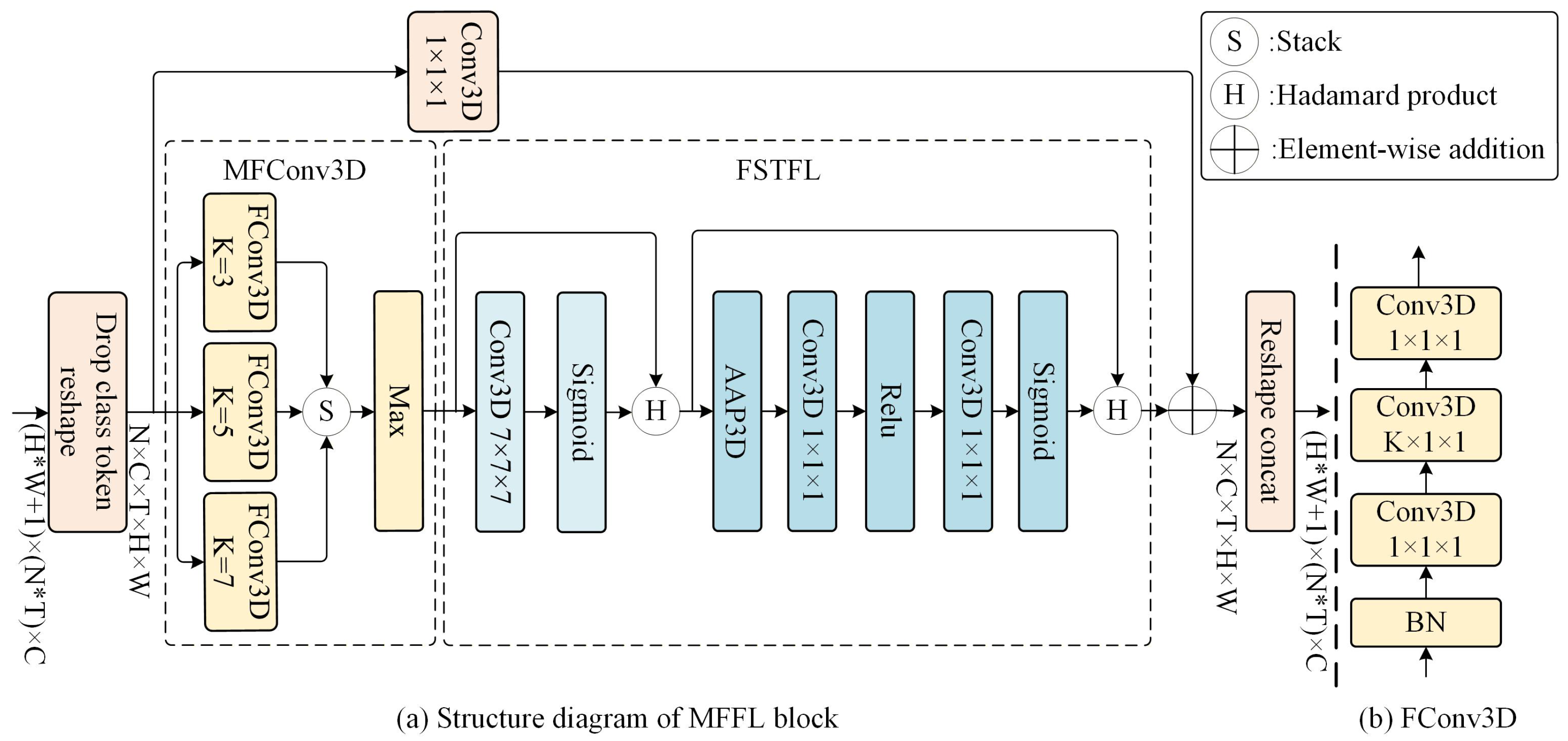
All 12 layers	126.36	69.48

presents the results. Given that deeper networks capture high-level abstract features such as semantics and context, embedding the MFFL block in deeper layers can enhance the ability to learn multiscale features of fire.

As shown in Table 5, we progressively increased the number of MFFL blocks, starting from the last layer and embedding them in the final 1 to 2, 3, 4, 5, and 6 layers. Performance declined as the number of layers increased beyond the final 4 layer. To avoid redundancy, subsequent experiments only embedded MFFL in the final 1 to 8, 1 to 10, and all 12 layers. A substantial performance gap exists between the “Final 1 to 3 layers” and “Final 1 to 4 layers” configurations. To validate the independent contribution of the 4th-to-last layer, a supplementary experiment was performed where the MFFL module was embedded exclusively in the 4th-to-last layer.

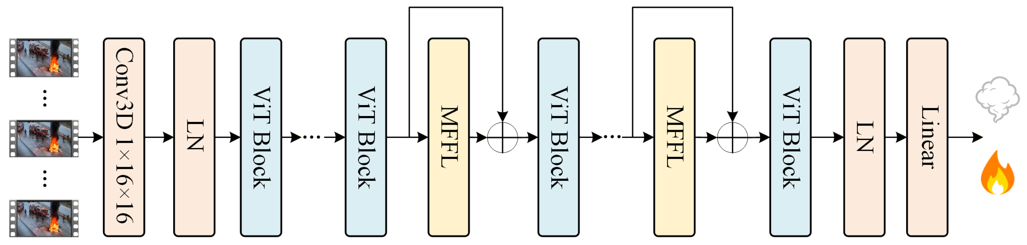
The best result is achieved when MFFL is embedded in the final 1 to 4 layers. These findings suggest that the position and quantity of MFFL blocks influence the performance. Concentrating the MFFL blocks in a limited number of deep layers improves recognition accuracy while reducing the number of parameters, thereby serving as an optimal configuration strategy. Consequently, MFFLNet embeds MFFL blocks in the final 1 to 4 layers of the ViT-B backbone.

To evaluate the contribution of MFConv3D and FSTFL within the MFFL block, ablation experiments were conducted on FSVR. The results are presented in

Table 6. Ablation experiments on the FSVR dataset.

Method	Backbone	Pre-Trained Weights	Acc (%)	Macro-F1 (%)
Baseline	ViT-B	Kinetics-710	$77.40\pm 0.39$	$76.95\pm 0.48$
FSTFL	ViT-B	Kinetics-710	$78.46\pm 0.27$	$78.08\pm 0.27$
FSTFL + MFConv3D	ViT-B	Kinetics-710	$79.54\pm 0.19$	$79.22\pm 0.15$

, where “Baseline” denotes the method that excludes the utilization of the proposed FSTFL and MFConv3D. All methods in this table were evaluated under identical experimental settings. Moreover, we conducted the experiment three times with distinct random seeds and report the mean ± standard deviation.

As presented in Table 6, the baseline method, with the integration of the FSTFL layer, yields an accuracy of 78.46% and a macro-F1 score of 78.08%, respectively. This finding demonstrates that FSTFL effectively captures the spatiotemporal features of flames and smoke. When the MFConv3D layer is further incorporated into the FSTFL-equipped method, the resulting accuracy and macro-F1 score are 2.14% and 2.27% higher than those of the baseline method, respectively. Notably, the standard deviation of the experimental results gradually decreases with the sequential addition of FSTFL and MFConv3D. This observation indicates that these two layers not only enhance the model’s capability to learn features of flames and smoke but also improve the stability of the experimental results. The ablation experiments demonstrate that the two layers effectively enhance the performance of the baseline method on the FSVR dataset, thereby validating the effectiveness of both layers.

5.5. Comparison with Other Methods

5.5.1. Comparison on FSVR

On the FSVR dataset, we compare the performance of MFFLNet against 4 classic methods, i.e., TimeSformer [43], VideoSwin [50], MViTv2 [48], and UniformerV2 [49]. For TimeSformer, the spatial-only model was used for testing.

Table 7. Comparison of other methods on FSVR.

Method	Backbone	Pre-Trained Weights	Training Frames	Acc (%)	Macro-F1 (%)
MViTv2 [48]	MViT-B	None	16	$56.30\pm 0.95$	$54.30\pm 0.71$
VideoSwin [50]	Swin-B	None	16	$57.08\pm 0.62$	$55.68\pm 0.81$
TimeSformer [43]	ViT-B	None	16	$58.00\pm 1.55$	$57.61\pm 2.16$
UniformerV2 [49]	ViT-B	None	16	$59.82\pm 0.13$	$58.57\pm 0.43$
MFFLNet	ViT-B	None	16	$60.58\pm 0.18$	$59.56\pm 0.99$
TimeSformer [43]	ViT-B	Kinetics-400	16	$69.89\pm 0.68$	$69.34\pm 1.11$
VideoSwin [50]	Swin-B	Kinetics-400	16	$71.35\pm 1.90$	$70.57\pm 2.24$
MViTv2 [48]	MViT-B	Kinetics-400	16	$72.41\pm 0.95$	$71.30\pm 1.14$
UniformerV2 [49]	ViT-B	Kinetics-400	16	$78.33\pm 0.88$	$77.86\pm 0.98$
MFFLNet	ViT-B	Kinetics-400	16	$78.66\pm 0.89$	$78.26\pm 0.94$
UniformerV2 [49]	ViT-B	Kinetics-710	8	$77.31\pm 0.18$	$76.70\pm 0.26$
UniformerV2 [49]	ViT-B	Kinetics-710	16	$78.01\pm 0.08$	$77.46\pm 0.10$
MFFLNet	ViT-B	Kinetics-710	8	$78.70\pm 0.21$	$78.26\pm 0.31$
MFFLNet	ViT-B	Kinetics-710	16	$79.54\pm 0.19$	$79.22\pm 0.15$

presents the comparative results across three experimental settings: “None” indicates that networks were not initialized with pre-trained weights; “Kinetics-400” refers to initializing networks with pre-trained weights obtained by the corresponding method on the Kinetics-400 [51] dataset; and “Kinetics-710” refers to initializing networks with pre-trained weights from the Kinetics-710 dataset. To save time, we directly used publicly available pre-trained weights from existing methods.

Under the experimental setup where no pre-trained weights are used and 16 frames are utilized, MFFLNet achieves an accuracy of 60.58% and a macro-F1 score of 59.56%, outperforming all other baseline methods. These experimental results demonstrate that the multiscale fire feature learning architecture of MFFLNet can effectively capture the visual variations and temporal dynamics of flames and smoke. During the training process, MFFLNet exhibits a robust ability to learn fire-related features without relying on large-scale external data for pre-training.

Under the experimental setup employing pre-trained weights from the Kinetics-400 dataset, the recognition performance of all methods in Table 7 was significantly enhanced. Under identical experimental settings, MFFLNet outperformed the other comparative methods. These results demonstrate that MFFLNet can effectively transfer general video features when leveraging the Kinetics-400 pre-trained weights.

When pre-trained weights from the larger-scale Kinetics-710 dataset are utilized, the performance of all methods is further enhanced. When only 8 frames are fed as input to the network, both metrics of MFFLNet surpass those of UniformerV2 that uses 16 frames. Generally, using fewer frames as input reduces the time complexity of the algorithm. This indicates that MFFLNet can improve training and inference speed by using fewer frames as input, while maintaining high recognition performance. In summary, MFFLNet achieves the best results on FSVR, demonstrating superior performance in the FVR domain.

5.5.2. Comparison on LFVR

To further validate MFFLNet, experiments were performed on the LFVR dataset.

Table 8. Comparison of other methods on LFVR.

Method	Backbone	Training Frames	Acc (%)	F1-Score (%)
TimeSformer [43]	ViT-B	32	85.67	81.14
VideoSwin [50]	Swin-B	32	89.40	86.41
I3D [51]	ResNet50	32	89.64	86.76
LGAE [9]	Swin-B	32	91.27	88.93
MFFLNet	ViT-B	16	95.34	95.17
MFFLNet	ViT-B	32	95.64	95.46

compares the performance of TimeSformer, VideoSwin, I3D [51], LGAE [9], and MFFLNet on LFVR. Following the previous study [9], 32 frames were employed as the input to the neural network. Similar to the experiments conducted on the FSVR dataset, we also present the experimental results of MFFLNet with 16 frames as input.

Generally, the method utilizing 32 frames as training input achieves superior performance compared to the same method employing 16 frames. With 16 frames as input, MFFLNet achieves an accuracy of 95.34% and an F1-score of 95.17%, outperforming other methods that utilize 32 frames. Despite using half the number of input frames compared to other approaches, MFFLNet can still precisely capture the dynamic features of fire via the proposed MFFL block. When 32 frames are employed as input, the performance of MFFLNet on the LFVR dataset is further enhanced. These experimental results demonstrate the superior performance of MFFLNet in the FVR task.

5.6. Time Complexity

Experiments were performed on the FSVR dataset to evaluate computational efficiency. The comparison results are shown in

Table 9. Comparison of time complexity on FSVR.

Method	Training Frames	Parameter (M)	GFLOPs	Training Time (s)	Testing Time (ms)	Acc (%)
MViTv2 [48]	16	50.92	185	641	60	$56.30\pm 0.95$
VideoSwin [50]	16	87.64	282	385	58	$57.08\pm 0.62$
TimeSformer [43]	16	85.80	563	1133	136	$58.00\pm 1.55$
UniformerV2 [49]	16	123.74	652	732	82	$59.82\pm 0.13$
MFFLNet	16	99.32	644	710	80	$60.58\pm 0.18$

, where “Parameter” denotes the number of network parameters, “GFLOPs” represents the number of floating-point operations, “Training Time” indicates the average training time per epoch in seconds, and “Testing Time” refers to the average inference time per sample in milliseconds. These experiments were conducted on two NVIDIA Tesla V100 GPUs.

As shown in Table 9, MViTv2 has the smallest parameter count, but suffers from significant shortcomings in performance. VideoSwin achieves the best training and testing speed, yet its accuracy remains limited. Compared to UniformerV2, MFFLNet achieves lower parameter count and computational cost. In terms of model performance, MFFLNet reaches an accuracy of 60.58% with a standard deviation of only 0.18, demonstrating excellent stability. Compared to high-accuracy models such as TimeSformer and UniformerV2, MFFLNet achieves significant performance improvement with comparable computational time. Overall, MFFLNet effectively balances model time complexity, computational cost, and recognition performance.

5.7. Discussion and Analysis

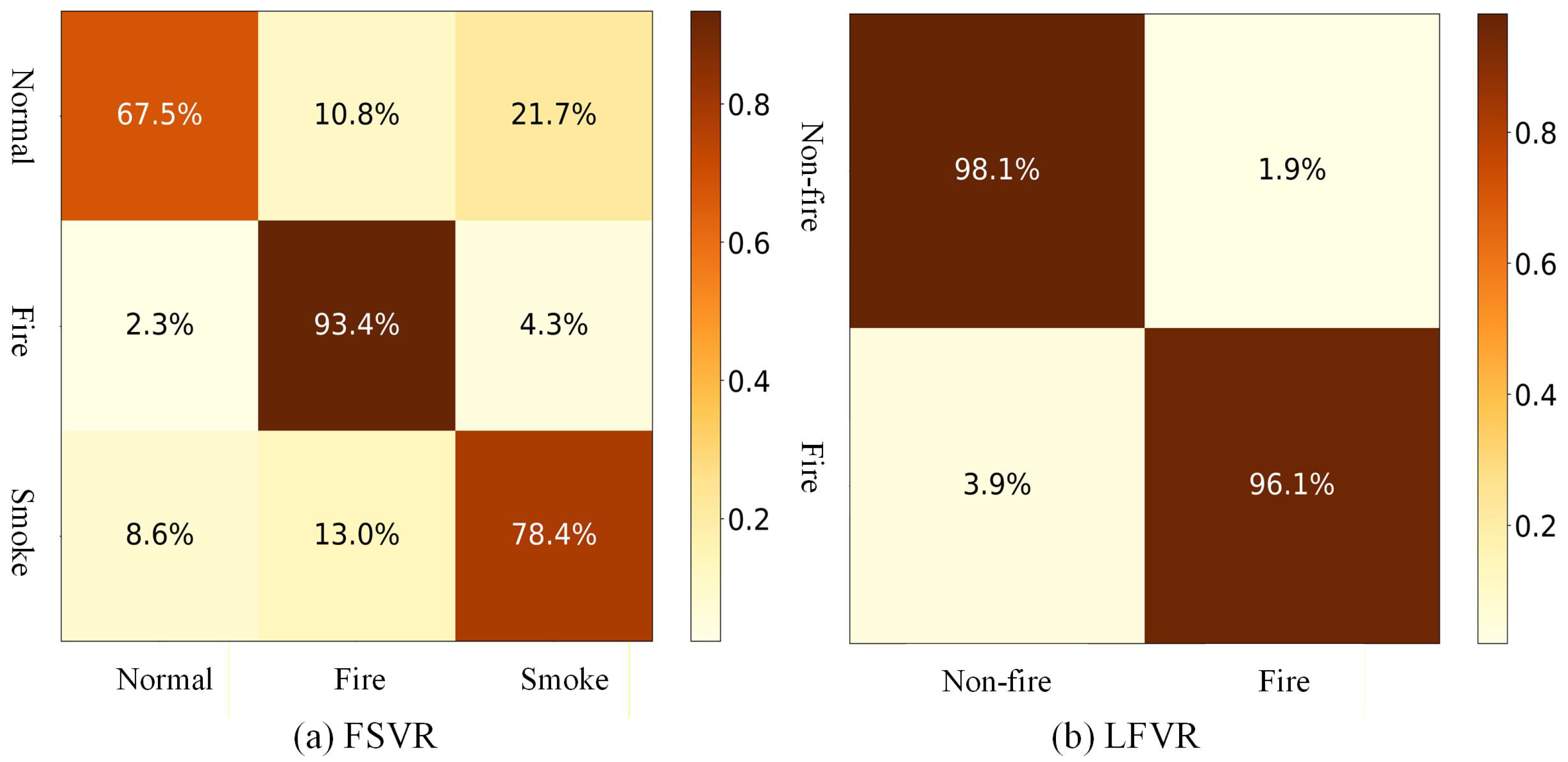
To further investigate the effectiveness of MFFLNet, two approaches are employed to visualize and analyze the experimental results. Figure 4 presents the confusion matrices for the FSVR and LFVR datasets.

As shown in Figure 4a, MFFLNet achieves the highest accuracy for the Fire category, with a value of 93.4%. This indicates that MFFLNet is capable of stably capturing the discriminative information associated with this category. The accuracies for the Normal and Smoke categories are 67.5% and 78.4%, respectively. Although significantly lower than that of the Fire category, these results remain acceptable given the inherent visual similarities between smoke and normal scenes.

While significantly lower than that of the Fire category, these results remain acceptable. The categories with the highest misclassification rates are Normal and Smoke. This is likely attributed to the visual similarity between smoke and certain normal scenes, which may result in misclassification under low-contrast or complex background conditions. As shown in Figure 4b, the accuracies for the Non-fire and Fire categories reach 98.1% and 96.1%, respectively, with cross-misclassification rates below 4%. These results demonstrate the outstanding performance of MFFLNet, exhibiting stable and excellent classification across both datasets. Moreover,

Table 10. Raw confusion-matrix counts of MFFLNet on FSVR.

	Normal	Fire	Smoke	Row Sum
Normal	4076	651	1309	6036
Fire	138	5546	256	5940
Smoke	517	782	4725	6024

reports the raw confusion-matrix counts of MFFLNet on FSVR.

The diagonal entries of Table 10 indicate the number of correctly classified samples, which are 4076 for Normal, 5546 for Fire, and 4725 for Smoke. Regarding misclassifications, 651 and 1309 Normal samples were incorrectly predicted as Fire and Smoke, respectively; 138 and 256 Fire samples were misidentified as Normal and Smoke, respectively; and 517 and 782 Smoke samples were erroneously classified as Normal and Fire, respectively. The row sums show that the total number of test samples per class is 6036, 5940, and 6024, indicating a relatively balanced class distribution. Overall, MFFLNet attains the highest recognition accuracy for the Fire class.

Table 11. A comparison of MFFLNet’s performance across three categories on FSVR.

Class	Precision (%)	Recall (%)	F1-Score (%)	Specificity (%)	FAR (%)	MDR (%)
Normal	86.16	67.53	75.71	94.53	5.47	32.47
Fire	79.47	93.37	85.86	88.12	11.88	6.63
Smoke	75.12	78.44	76.74	86.93	13.07	21.56

presents a comparison of MFFLNet’s performance across three categories on FSVR. Experimental results demonstrate that MFFLNet exhibits the optimal detection performance in the Fire category, achieving a recall of 93.37% and an F1-score of 85.86%, with a corresponding Missed-Detection Rate (MDR) of merely 6.63%. This underscores the model’s robust capability in fire recognition, which effectively ensures a high detection rate for fire. The F1-scores for the Smoke and Normal categories are 76.74% and 75.71%, respectively, indicating that their overall performance lags behind that of the Fire category. The Normal category achieves a specificity of 94.53% and a relatively low False Alarm Rate (FAR) of 5.47%, though its MDR remains comparatively high. The Smoke category, by contrast, has the highest FAR among the three at 13.07%. This discrepancy is closely tied to the properties of smoke, including its variable morphology, ambiguous texture features, and proneness to confusion with fog and other interfering factors. A primary direction for future optimization will be to enhance the smoke feature representation capability, thereby reducing the MDR and improving overall detection performance.

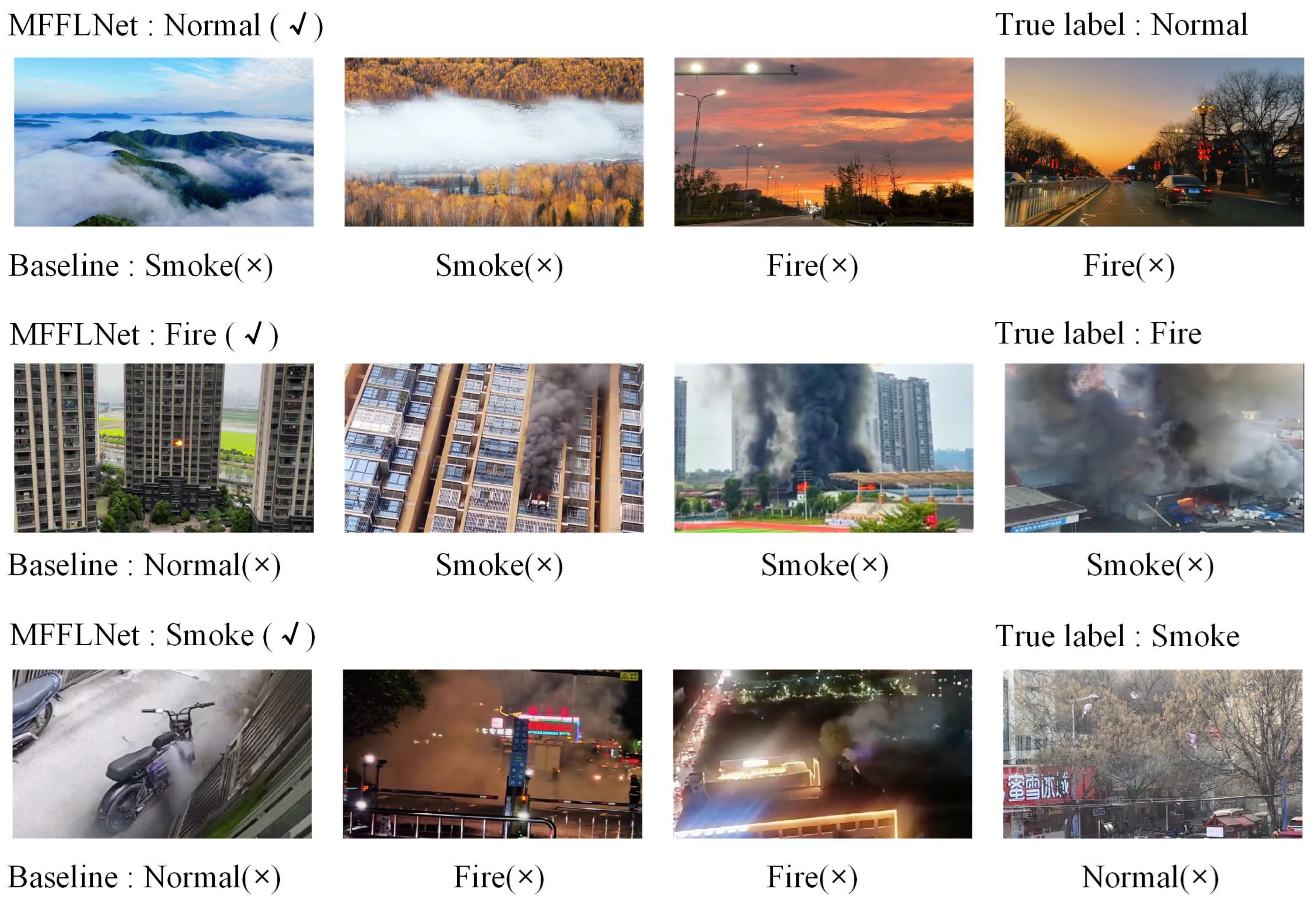
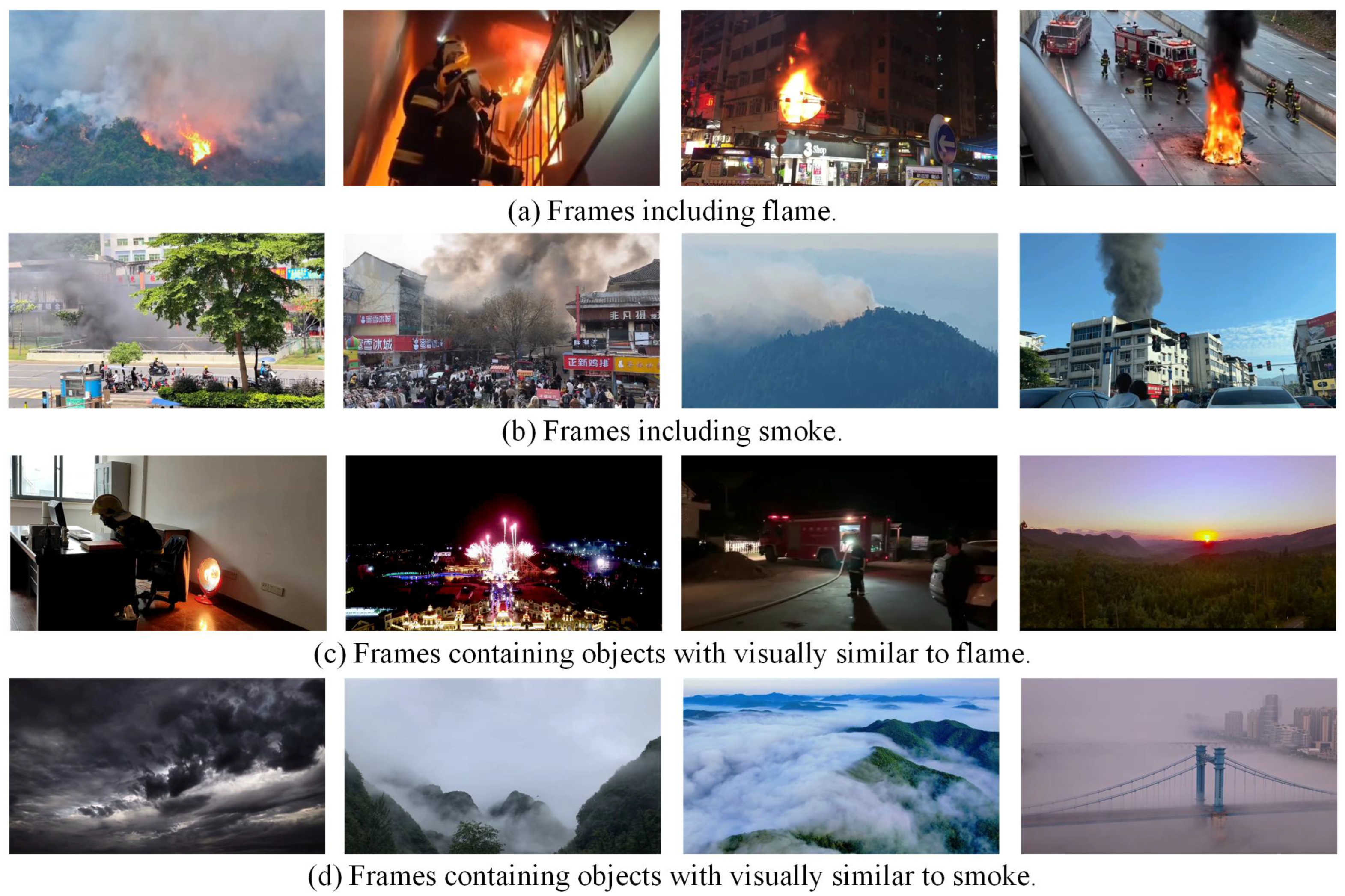
Figure 5 presents typical cases where MFFLNet predicts correctly while the baseline method fails, covering the Normal, Fire, and Smoke categories in the FSVR dataset. For the Normal category, the baseline method is susceptible to interference from smoke-like and flame-like backgrounds, such as mountain clouds, mist, dusk glow, night road scenes, etc. For the Fire category, the baseline method fails to recognize small-area flame and early-stage fire. For the Smoke category, the baseline method exhibits missed detection issues when identifying weak and diffuse smoke, and is prone to confusing smoke with fire. The comparative results demonstrate that MFFLNet exhibits superior FVR capability, achieving robust and accurate classification performance across multiple scenarios.

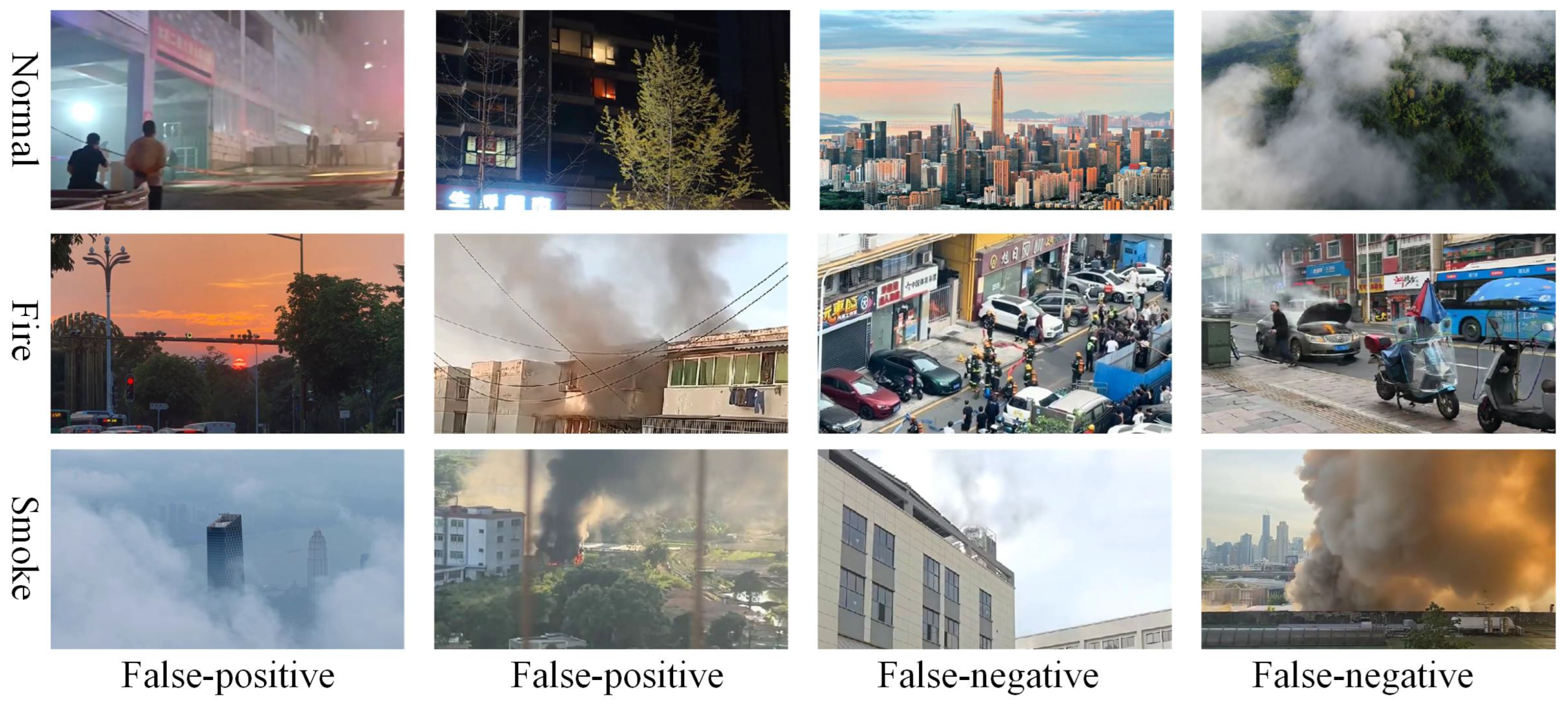
Figure 6 presents representative False-Positive (FP) and False-Negative (FN) instances of MFFLNet on the FSVR dataset. These samples are primarily attributed to environmental interference, and their visual characteristics resemble those of flames and smoke, such as clouds, fog, sunlight at dawn or dusk, dust from construction sites, and warm light sources at night.

Moreover, FP and FN samples also appear in scenarios involving small-scale, distant, or occluded objects. When smoke or flames occupy a relatively small area in the image, are partially occluded by structures such as buildings, or exist under low-contrast lighting conditions, the model struggles to extract sufficiently prominent and discriminative features. These failure cases highlight the model’s limitations in complex real-world scenarios.

To reduce false alarm rates, future research will focus on two aspects. First, the fine-grained feature decoupling and adversarial discriminative learning algorithms will be developed to distinguish fire from environmental interference at the representation level. Second, the multi-resolution local attention and temporal context modeling algorithms will be developed to enhance the recognition capabilities for fires in scenarios involving small targets, long distances, and occlusions.

6. Conclusions

To advance research in the field of FVR, the large-scale FSVR dataset was constructed. To better utilize multiscale information for FVR, we proposed the Transformer-based MFFLNet, which integrates multiple MFFL blocks. Extensive experiments were conducted on the FSVR and LFVR datasets. These results indicate that MFFLNet outperforms the baseline methods and achieves the best results in the FVR field. Future work will explore the integration of motion information from flame and smoke for more precise recognition. Furthermore, we aim to expand the dataset by collecting a more extensive range of fire videos across diverse scenarios.