Performance and Emissions Assessment of a Micro-Turbojet Engine Fueled with Jet A and Blends of Propanol, Butanol, Pentanol, Hexanol, Heptanol, and Octanol

Abstract

This study examines the impact of alcohol blends on the performance and emissions of aviation micro-turbojet engines. Thus, propanol, butanol, pentanol, hexanol, heptanol, and octanol were tested at 10%, 20%, and 30% concentrations and mixed with Jet A, as well as with an additional 5% heptanol blend to preserve base fuel properties, to fuel a JetCat P80 micro-turbojet. Physicochemical properties such as density, viscosity, and elemental composition were analyzed before engine testing. Carbon dioxide (CO₂) emissions from 1 kg of fuel combustion varied, with propanol yielding the lowest at 3.02 kg CO₂ per kg of fuel and octanol yielding the highest at 3.22 kg CO₂ per kg of fuel. The following results were obtained: alcohol blends lowered exhaust gas temperature by up to 7.5% at idle and intermediate thrust but slightly increased it at maximum power; fuel mass flow increased with alcohol concentration, peaking at 20.4% above Jet A for 30% propanol; and thrust varied from −4.92% to +7.4%. While specific fuel consumption increased by up to 12.8% for propanol, thermal efficiency declined by 1.8–5.6% and combustion efficiency remained within ±2% of Jet A. Butanol and octanol emerged as viable alternatives, balancing emissions reduction and efficiency. The results emphasize the need for an optimal trade-off between environmental impact and engine performance.

1. Introduction

The aviation industry is facing increasing pressure to reduce its environmental footprint, playing a crucial role in global efforts to combat climate change [1]. As one of the major consumers of fossil fuels, aviation represents a strategic sector in the exploration of sustainable energy solutions [2]. In this context, recent research has identified several alternatives for aviation fuels, including the use of alcohols, hydrogen (in both liquid and gaseous forms), and synthetic fuels [3,4,5,6]. Currently, the most advanced studies in aviation fuels focus on the development and implementation of biofuels, which have proven to be more environmentally friendly and hold significant potential in reducing greenhouse gas emissions and CO₂ concentrations [7].

In addition to biofuels, alcohols may present a viable option for enhancing the characteristics of aviation fuels. Alcohols are attractive additives due to their high oxygen content, which promotes cleaner combustion, in turn reducing carbon monoxide (CO), particulate matter (PM), and other harmful emissions. Their integration into blends with conventional jet fuels could help to achieve more eco-friendly aviation fuels [8]. However, alcohols exhibit inferior properties when compared with traditional aviation fuel Jet A, as detailed in [9]. This study investigated the physical properties of Jet A fuel mixed with n-heptane and various n-alcohols (n-propanol, n-butanol, n-pentanol, n-hexanol, n-heptanol, and n-octanol), using blends with concentrations of 10%, 20%, and 30%. Alcohols derived from biomass or with bio-production potential were evaluated according to ASTM D1655 standards for density, viscosity, and flash point. Refractive index measurements and FTIR analysis provided additional information about the chemical composition of the blends. Their density met ASTM specifications, and viscosity extrapolation suggested compliance with the standards. Furthermore, regression equations were developed to estimate density, viscosity, and refractive index, with correlations showing R² values above 0.99.

Compared with the use of alcohols in piston engines [10,11], studies on alcohol blends with Jet A in turbojet engines are less frequent.

One such study is presented in [12], where the effect of methanol on microturbine performance is analyzed, evaluating blends with methanol concentrations of 10%, 20%, and 30% under different operating conditions. The results indicate that 10% and 20% methanol blends provide stable performance, while 30% methanol concentrations lead to instability, especially at maximum speeds. The study also examines emissions generated, highlighting the feasibility of using methanol in aviation at lower concentrations. In [13], the use of butanol in microturbines is investigated by testing various concentrations of n-butanol and assessing the effects on engine performance and emissions of sulfur dioxide (SO₂) and carbon monoxide (CO). The results show that n-butanol/Jet A blends improve combustion efficiency and reduce emissions compared with conventional Jet A fuel, with higher n-butanol concentrations leading to further reductions in SO₂ and CO emissions. This study thus supports the use of n-butanol as a promising SAF in Jet A blends for more environmentally friendly aviation operations.

Further, in [14], tests are presented on the performance of microturbines using blends with 10%, 20%, and 30% ethanol under varying operating conditions, such as idle, cruise, and full power. The results suggest that ethanol–kerosene blends provide stable engine performance and significantly reduce pollution, thereby supporting the idea that these blends represent an efficient SAF for micro-turbo engines. In [15], ethanol is explored as an alternative for small turbojet engines (up to 2 kN), using ethanol–Jet A-1 blends in laboratory conditions. The study highlights that ethanol is effectively usable only at concentrations below 40%, having beneficial effects on operating temperatures but with a limited impact on engine speed and thrust.

Moreover, in [16], the impact of butanol/Jet A blends on gas turbine engine performance and emissions is analyzed, with results indicating a reduction in NOx and CO emissions but also a decrease in the operational thrust range compared with pure Jet A. In [17], emissions of gaseous pollutants and particles from a gas turbine burner using blends of butyl butyrate and ethanol are examined. Compared with aviation kerosene (RP-3), biofuels generated higher CO emissions due to lower combustion temperatures but reduced NOx and UHC emissions, especially when ethanol concentrations were higher.

In [18], the combustion characteristics of Jet A-1 and a 10% butanol–Jet A-1 blend are compared using a miniaturized turbojet engine test rig. The results highlight significant differences in engine performance and exhaust gas emissions, contributing to the further exploration of alternative fuels for aviation. Finally, the paper in [19] analyzes the use of butanol/biobutanol as a bio-component in aviation and diesel fuels, considering the growing need for sustainable alternatives in air transport. Tests on Jet A-1 and diesel blends with butanol isomers (0–20%) suggest that butanol can become a promising precursor for the production of biohydrocarbons in aviation fuels.

The findings of the reviewed studies reveal important insights into the performance, emissions, and fuel properties of various aviation fuel blends.

Regarding performance, the combustion temperature of Jet A–biodiesel blends in-creases at idle but decreases at intermediate and maximum regimes [5]. Similarly, the use of a Jet A–n-butanol blend results in a 2% reduction in exhaust gas temperature [18]. Thrust is significantly impacted when using a Jet A–n-butanol blend, with a notable 35% reduction compared with pure Jet A [18]. Specific fuel consumption increases as well, rising by more than 4% with a higher biodiesel concentration [5] and by almost 3% when using a Jet A–n-butanol blend instead of pure Jet A [18].

In terms of emissions, the studies highlight several key benefits of alternative fuels. Carbon dioxide (CO₂) emissions decrease by 2.2% as biodiesel concentration increases [5] and by 2% when using a Jet A–n-butanol blend [18]. More notably, sugarcane-derived microbial oil has the potential to reduce greenhouse gas (GHG) emissions by over 50% compared with fossil fuels [7]. Carbon monoxide (CO) emissions are also reduced, showing a 5% decrease when using the Jet A–n-butanol blend [18], while nitrogen oxide (NOx) emissions see a 2% reduction under the same conditions [18]. The chemical structure of the alcohols plays a significant role in PM emissions, with longer-chain alcohols such as 2-ethylhexanol and 1-octanol proving more compatible with fuel and leading to lower particle emissions, whereas ethanol presents combustion and emission challenges due to its high volatility and low cetane number [10].

When examining fuel properties and suitability, it was found that Jet A–alcohol blends (ranging from propanol to octanol) exhibit only a minor density variation of 1.7%, remaining within the interval of 0.7939–0.8075 g/cm³ and meeting ASTM requirements for sustainable aviation fuel [9]. Furthermore, in terms of feedstock efficiency, sugar-cane-derived microbial oil demonstrates significant advantages, producing approximately four times more SAF per unit area compared with soybean oil [7].

These findings collectively underline the viability of alternative aviation fuels in terms of performance, emissions reduction, and compliance with fuel standards, sup-porting further exploration of bio-based fuel solutions for sustainable aviation.

The current paper aims to investigate and analyze the impact of using various alcohols—propanol, butanol, pentanol, hexanol, heptanol, and octanol—in blend ratios of 10%, 20%, and 30% with Jet A as fuel for aviation micro-turbojet engines, specifically testing these mixtures in a JetCat P80 engine while also incorporating 5% heptanol to mitigate excessive alterations to the base fuel properties; the research is structured into three phases: first, analyzing the physicochemical properties of the blends, including density, viscosity, flammability, and elemental composition; second, calculating the CO₂ emissions per kilogram of fuel burned based on elemental concentrations and comparing the seven studied blends at different alcohol percentages; and third, conducting experimental tests on the micro-turbojet to evaluate combustion gas temperature before the turbine, fuel flow rate, thrust, specific fuel consumption, combustion and thermal efficiency, and measuring CO concentrations in the exhaust using a gas analyzer. This is the first experimental design to assess so many alcohol blends (6) with so many concentrations (3) and working with so many engine regimes (3). In this manner, this paper can be considered the starting point of an even wider database that can be formed in the future.

2. Materials and Methods

2.1. Materials and Mixture Preparation

For this research, Jet A fuel, containing additives, was sourced from a local company. Aeroshell 500 engine lubrication oil was provided by Shell Romania (Bucharest, Romania). n-Heptane (≥99% purity) was purchased from Lach-Ner (Neratovice, Czech Republic). The information regarding the alcohols is listed in

Table 1. Information of various alcohols.

Properties	Unit	Propanol	Butanol	Pentanol	Hexanol	Heptanol	Octanol
Chemical formula	-	C3H7OH	C4H9OH	C5H11OH	C6H13OH	C7H15OH	C8H17OH
Purity	%	≥99.5	99.5	≥99	98	98	≥99
Provider		Lach-Ner	Chemical	Honeywell (Bucharest, Romania)	Sigma-Aldrich (Burlington, MA, USA)	Sigma-Aldrich	Sigma-Aldrich

.

Mixtures were prepared with volumetric measurements (accuracy ±0.01 mL), stirred to ensure miscibility, and stored in hermetically sealed containers. No phase separation was observed.

Viscosity, a measure of a liquid’s resistance to flow, is a critical parameter for fuel performance, especially at low temperatures. Dynamic viscosity is measured at 25 °C according to ASTM D7042 [20], using an Anton Paar SVM 3000 viscometer with specified uncertainty (±0.54%) (Anton Paar, Graz, Austria). The viscometer measures the friction force between the rotating cylinder and the liquid.

Density, the mass per unit volume, is a crucial parameter affecting fuel atomization. It is measured at 25 °C according to ASTM D7042 using an oscillating U-tube method (Anton Paar SVM 3000). A small sample is introduced into the tube, ensuring no bubbles are present. The change in the tube’s oscillation frequency, caused by the sample’s mass displacing the reference material, is directly related to its density. This method provides high uncertainty (±0.07%), with digital readings available to four significant figures.

The Anton Paar SVM 3000 viscometer uses a Peltier element to maintain sample temperature. It takes three measurements for each sample to guarantee result reliability as per ASTM standards.

To assess volatility, the distillation curves for Jet A and studied blends were determined using the ASTM D86 [21] method with an OPTIDIST™ automatic apparatus at atmospheric pressure (Optidist, Sofia, Bulgaria). Samples of 100 mL were heated at a rate of 5 mL/min. Distillation temperatures were recorded at the first drop at 5, 10, 15, 20, 30, 40, 50, 60, 70, 80, 90, and 95% volume distilled, with a volume measurement uncertainty of ±0.015 mL.

2.2. Analysis Procedures

2.2.1. Analysis of the Combustion Process of the Mixtures

With the elemental analysis determined, it is possible to calculate several key parameters resulting from the stoichiometric combustion of the fuels with air. Thus, the calculation considers the general formula C_cH_hO_oN_n [22], with specific fractions of g_C, g_H, g_O and g_N.

To understand the combustion process, it is crucial to know the minimum amount of oxygen required for combustion, as shown in Equation (1), followed by the amount of air necessary for combustion, as seen in Equation (2). Furthermore, an essential part of combustion analysis is determining the amount of CO₂ produced, as shown in Equation (3), as well as the amount of water generated from the combustion process, described in Equation (4).

$$M_o=2.667gC+8gH-gO$$

(1)

$$M_{air}=4.35M_o$$

(2)

CO₂ and H₂O from the combustion process can be calculated by using the following:

$$C{O}_2=44{\displaystyle \frac{gC}{12}}$$

(3)

$$H_{2}O=9gH$$

(4)

2.2.2. Jet Cat P80 Experimental

The experiments were conducted using a Jet Cat P80 micro-turbojet engine (JetCat, Ballrechten-Dottingen, Germany), as shown in Figure 1a. A detailed description of the micro-turbojet engine can be found in [23].

This micro-turbojet engine is equipped with instrumentation capable of measuring engine speed, air flow rate, fuel flow rate, thrust, combustion chamber pressure, temperature before the turbine, and temperature after the compressor. The acquisition rate is 1 signal per second. The tests were conducted at three different regimes: idle, intermediate, and maximum speed. The rotational speed for regime 1 is 35,000 rpm, for regime 2 is 55,300 rpm, and for regime 3 is 111,500 rpm. Due to the low signal acquisition rate, the tests were carried out over a period of approximately two minutes, with signal averaging performed during this time. This period was also necessary for measuring exhaust emissions.

For the measurements, classical instruments were used: type K thermocouples for temperature measurement, and, for the measurement of the nozzle pressure at the air inlet, a static pressure sensor with root extraction, made with the UNICON-P pressure converter produced by GHM GROUP—Martens, Germany, was used. For the measurement of the pressure in the combustion chamber, a pressure sensor with root extraction from Huba Control, Würenlos, Switzerland, was used. The tractive force was measured with a KM701 K 200 N 000 Z force transducer with 2 mV/N, manufactured by MEGATRON Elektronik GmbH & Co. KG, Putzbrunn, Germany. The speed was measured with a tachometer, and the fuel flow rate was determined based on the consumption measured by the fuel pump actuator.

The parameters of interest for our study are the temperature before the turbine, fuel flow rate, and thrust. A detailed description of the micro-turbojet engine and the test stand can be found in [24].

Gas emissions measurements were performed using an MRU Vario Plus analyzer (Messgeräte für Rauchgase und Umweltschutz GmbH, Neckarsulm-Obereisesheim, Germany), as shown in Figure 1b. The analyzer simultaneously measured various gas components, particularly CO and SO₂. The detection range for sulfur dioxide (SO₂) was 0–2000 ppm with an accuracy of ±10 ppm or 5%; for carbon monoxide (CO), the range was 0–4000 ppm with an accuracy of ±10 ppm or 5%; and for NO_x, the range was 0–200 ppm with an accuracy of ±5 ppm or 5%.

2.3. Calculating Micro-Turbojet Engine’s Performance

The most critical performance metrics that can be derived solely from experimental data are the specific fuel consumption, which is an essential parameter characterizing the performance of turbine engines, combustion efficiency, and thermal efficiency. To determine these values, a set of equations is applied [25].

For calculating specific fuel consumption, Equation (5) is used. As the micro-turbine instrumentation measured both the fuel flow rate and thrust force, the specific fuel consumption can be derived directly from these measured values. In Equation (5), F represents the measured thrust force in [N], and Mf is the fuel flow rate in [kg/s].

Regarding the calculation of specific consumption (S), Equation (5) is used.

$$S=3600·{\displaystyle \frac{\dot{M}f}{F}}\left[{\displaystyle \frac{kg}{N·h}}\right]$$

(5)

$\dot{M}f$ is the fuel flow rate expressed in kg/s, while F is the thrust force generated by the micro-turbine engine in [N]. As the micro-turbine instrumentation records fuel flow in L/s, it is necessary to know the density of each fuel, which is determined in the laboratory.

Based on the data recorded by the micro-turbine instrumentation, the combustion efficiency is determined using Equation (6).

$${\eta }_b={\displaystyle \frac{\left(\dot{M}f+\dot{M}a\right)c{p}_{3\_comb}·T_{\_comb}-\dot{M}a·c{p}_{\_comp}·T_{\_comp}}{\dot{M}f·LCP}}$$

(6)

In this formula, LCP is the lower calorific value, Tcomb is the temperature recorded in front of the turbine (at the exhaust of the combustion chamber), Tcomp is the temperature recorded in front of the combustion chamber (after the compressor), Ma is the air flow rate in [kg/s], and cp comp and cp comb are the specific heat capacities of the air at the compressor outlet and of the combustion gases at the combustion chamber outlet, corresponding to the recorded temperatures.

To determine thermal efficiency, Equation (7) is applied, where all of the parameters are either measured or derived from the data recorded by the micro-turbine instrumentation.

$${\eta }_T={\displaystyle \frac{\left(\dot{M}a+\dot{M}f\right)·v_e^2}{2·\dot{M}f·LCP}}={\displaystyle \frac{\left(\dot{M}a+\dot{M}f\right)·{\left(\frac{F}{\dot{M}a+\dot{M}f}\right)}^2}{2·\dot{M}f·LCP}}$$

(7)

Here, v_e represents the exhaust velocity of the combustion gases from the reaction nozzle.

3. Results and Discussion

3.1. The Experimentally Determined Values for the Physical–Chemical Properties

3.1.1. Density and Dynamic Viscosity Measurements

The density of the Jet A sample at 25 °C is 0.7825 g/cm³ and the dynamic viscosity at 25 °C is 1.0399 mPa·s. Experimental density and dynamic viscosity, of the pseudo-ternary mixtures, measured at 25 °C and atmospheric pressure is presented in

Table 2. Experimental density (g/cm³) and dynamic viscosity (mPa·s), of the pseudo-ternary mixtures, measured at 25 °C and atmospheric pressure.

Percent [%]	Properties	Propanol	Butanol	Pentanol	Hexanol	Heptanol	Octanol
10%	Density at 25 °C	0.7880	0.7897	0.7909	0.7912	0.7919	0.7954
	Viscosity at 25 °C	1.1167	1.1576	1.2043	1.2390	1.2716	1.3724
20%	Density at 25 °C	0.7895	0.7920	0.7934	0.7942	0.7950	0.7971
	Viscosity at 25 °C	1.1943	1.2506	1.3411	1.3937	1.4780	1.6069
30%	Density at 25 °C	0.7922	0.7942	0.7965	0.7975	0.7991	0.8009
	Viscosity at 25 °C	1.2920	1.3568	1.4831	1.6288	1.7131	1.9125

.

An increase in the carbon chain length of the alcohol components leads to a corresponding rise in both the sample density and dynamic viscosity. Furthermore, as the alcohol concentration within the mixture increases, both the density and dynamic viscosity of the resulting blend also increase. This phenomenon can be attributed to the higher density and viscosity of the alcohol components compared with the other constituents of the mixture.

According to Ozsezen et al. [26], increased fuel density can alter the compression process, advancing injection timing and shortening ignition delay, which may result in higher NO_x emissions. According to Subhadip et al. [27], fuel viscosity significantly impacts combustion by altering spray properties, influencing evaporation, and heat transfer. Higher viscosity leads to larger droplets, potentially increasing NO_x and CO emissions, and causing injector deposits, soot formation, and particulate matter (PM). Poor atomization from high viscosity results in incomplete combustion, further contributing to emissions.

3.1.2. Distillation Curve

A distillation curve illustrates the relationship between boiling temperature and the percentage of volume distilled from a mixture. The initial fraction (0–20% v/v) indicates cold start, warm-up, evaporative emissions, and vapor lock tendencies. The mid-range fraction (20–90% v/v) reveals fuel performance during warm-up, acceleration, and cold weather conditions. The final fraction (90% v/v to endpoint) estimates the fuel’s scaling potential [28,29]. ASTM distillation was performed on Jet A and all alcohol blends. Distillation temperatures were recorded at the initial boiling point, 5, 10, 15, 20, 30, 40, 50, 60, 70, 80, 90, and 95% evaporation, and the final boiling point.

Figure 2 presents the boiling points of Jet A and the blends.

The volatility of the blends varied according to alcohol content. As illustrated in Figure 2, the distillation profile of Jet A exhibited a smooth and consistent increase from 157 °C to 234.5 °C. With the exception of the propanol blend, the distillation temperature trends were similar across all blends. The addition of propanol to Jet A resulted in an increase in boiling temperatures within the 5–30% v/v range of the distillation curve, signifying increased volatility. Following the evaporation of propanol, the boiling temperature increased rapidly, converging with the original Jet A distillation curve.

3.2. The Results of Theoretical Combustion Process

Other parameters of interest for the new fuels that were determined are presented in the table below, specifically the lower heating value and elemental analysis. Elemental analysis and lower heating value is presented in

Table 3. Elemental analysis and lower heating value.

Fuel		%	O2 [kg]	Air [kg]	CO2 [kg]	H2O [kg]	Pci [MJ/kg]
Jet A	C	85.17	3.322	14.450	3.123	1.198	42.40
	H	13.31
	O	1.45
	N	0.07
Propanol	C	60	2.407	10.471	2.200	1.208	30.50
	H	13.42
	O	26.67
Jet A+10%	C	82.59	3.240	14.095	3.029	1.211	41.32
	H	13.46
	O	3.9
Jet A+20%	C	80.08	3.149	13.697	2.936	1.212	40.13
	H	13.47
	O	6.422
Jet A+30%	C	77.56	3.057	13.299	2.844	1.213	38.94
	H	13.48
	O	8.944
Butanol	C	64.86	2.594	11.286	2.378	1.216	33.1
	H	13.51
	O	21.62
Jet A+10%	C	83.08	3.259	14.177	3.047	1.212	41.58
	H	13.46
	O	3.39
Jet A+20%	C	81.05	3.186	13.860	2.972	1.214	40.65
	H	13.48
	O	5.41
Jet A+30%	C	79.02	3.113	13.544	2.898	1.215	39.72
	H	13.50
	O	7.43
Pentanol	C	68.96	2.770	12.049	2.529	1.241	34.5
	H	13.79
	O	17.24
Jet A+10%	C	83.49	3.277	14.253	3.062	1.214	41.72
	H	13.49
	O	2.96
Jet A+20%	C	81.87	3.221	14.013	3.002	1.219	40.93
	H	13.54
	O	4.54
Jet A+30%	C	80.25	3.166	13.773	2.943	1.223	40.14
	H	13.59
	O	6.11
Hexanol	C	71.98	2.908	12.648	2.640	1.268	36
	H	14.09
	O	13.93
Jet A+10%	C	83.79	3.290	14.313	3.073	1.217	41.87
	H	13.52
	O	2.63
Jet A+20%	C	82.47	3.249	14.133	3.024	1.224	41.23
	H	13.60
	O	3.87
Jet A+30%	C	81.15	3.207	13.952	2.976	1.231	40.59
	H	13.68
	O	5.12
Heptanol	C	74.29	3.010	13.095	2.724	1.286	37
	H	14.29
	O	11.42
Jet A+10%	C	84.02	3.301	14.357	3.081	1.219	41.97
	H	13.54
	O	2.37
Jet A+20%	C	82.94	3.269	14.222	3.041	1.228	41.43
	H	13.64
	O	3.37
Jet A+30%	C	81.85	3.238	14.086	3.001	1.236	40.89
	H	13.74
	O	4.37
Octanol	C	76.17	3.086	13.426	2.793	1.293	38
	H	14.37
	O	9.46
Jet A+10%	C	84.21	3.308	14.391	3.088	1.220	42.07
	H	13.55
	O	2.179
Jet A+20%	C	83.31	3.285	14.288	3.055	1.229	41.63
	H	13.66
	O	2.98
Jet A+30%	C	82.41	3.261	14.186	3.022	1.239	41.19
	H	13.76
	O	3.781

.

By comparing the amounts of CO₂ calculated from the stoichiometric reactions, it can be observed that blends using propanol produce less CO₂ than the others containing alcohols with higher carbon content and, at the first glance, propanol seems to emerge as the optimal alcohol to be used in mixtures with Jet A. However, propanol also presents the lowest value for lower heating value, which will be reflected in the engine performance tests, as will be observed later. Conversely, octanol has the highest lower heating value but also produces the highest amount of CO₂.

3.3. The Results of Micro-Turbojet Engine Experiments

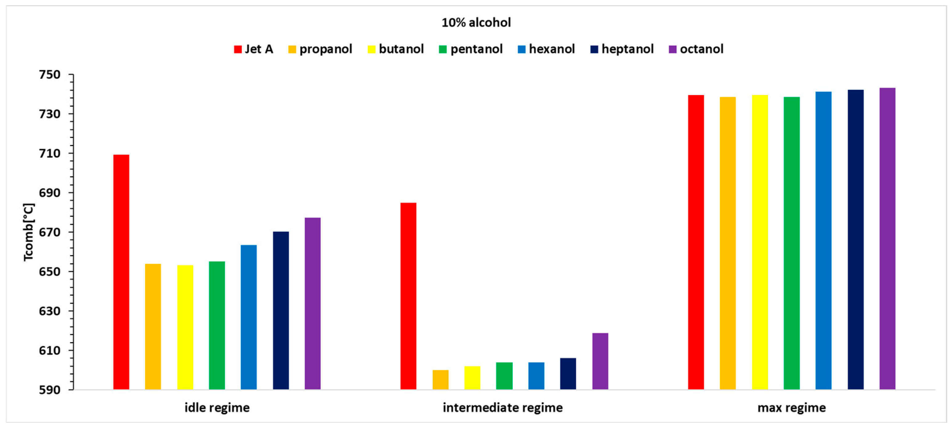
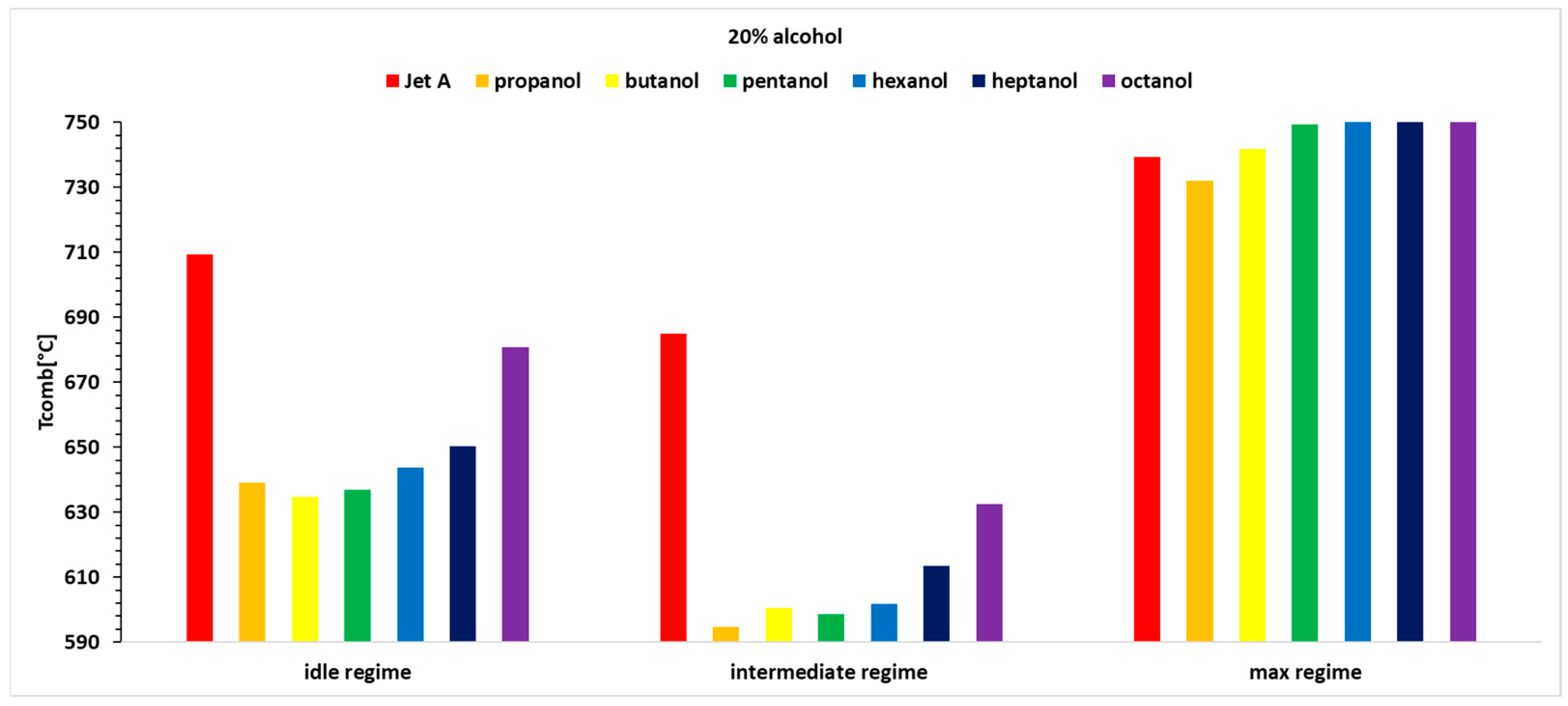
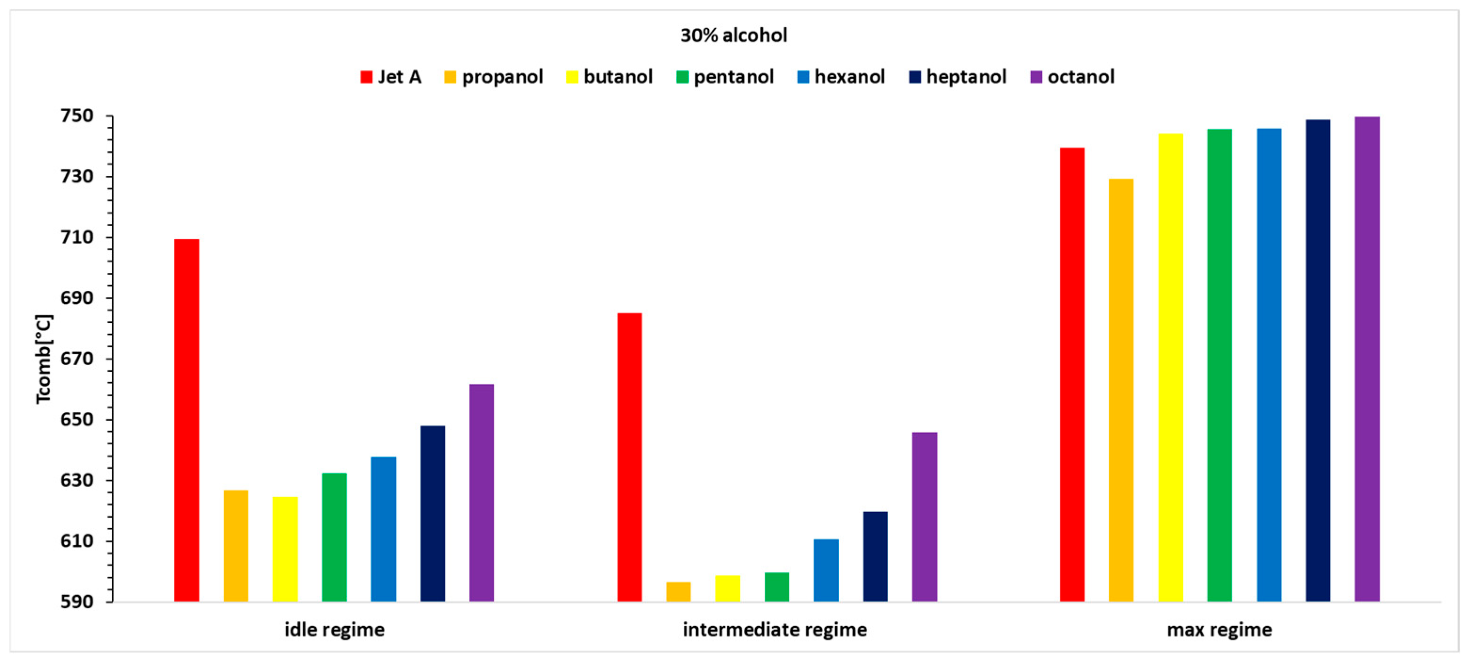
The following section presents the variation of the main parameters recorded during the operation of the micro-turbojet engine. Figure 3, Figure 4 and Figure 5 show the variations in exhaust gas temperature before the turbine for the three operating regimes of the micro-turbojet engine. Thus, Figure 3 illustrates the variation of the exhaust gas temperature before the turbine.

Analyzing Figure 3, Figure 4 and Figure 5, it can be observed that the exhaust gas temperature for the first two regimes and for all three alcohol concentrations is lower than the exhaust gas temperature when using the base fuel Jet A. This can be explained by the lower calorific value of the alcohols compared with Jet A. In the third regime, the exhaust gas temperature before the turbine increases slightly as the carbon content in the alcohols increases.

A detailed analysis is presented in

Table 4. Percentage variation of exhaust gas temperature before the turbine for the three studied regimes and all analyzed fuels.

Alcohol Percent [%]	Fuel	Propanol	Butanol	Pentanol	Hexanol	Heptanol	Octanol
	Regime	Variation [%]
10%	1	−7.81	−7.93	−7.66	−6.50	−5.53	−4.53
	2	−12.40	−12.11	−11.82	−11.82	−11.53	−9.65
	3	−0.12	0.02	−0.13	0.24	0.37	0.50
20%	1	−9.90	−10.52	−10.21	−9.24	−8.32	−4.02
	2	−13.18	−12.32	−12.62	−12.15	−10.43	−7.67
	3	−1.00	0.32	1.33	1.47	1.65	1.70
30%	1	−11.66	−11.96	−10.87	−10.12	−8.67	−6.73
	2	−12.91	−12.61	−12.47	−10.85	−9.55	−5.72
	3	−1.40	0.63	0.84	0.86	1.24	1.39

, which shows the percentage variation of the exhaust gas temperature before the turbine when using 10%, 20%, and 30% blends of the six alcohols for the three analyzed regimes. All of the tabulated data use as a reference baseline the temperatures obtained while using Jet A alone. The results have been obtained using Equation (8).

$$ariation \left(\%\right)=100-[\left({\displaystyle \frac{T_{Jet-A}}{T_{Blend}}}\right)\ast 100]$$

(8)

Analyzing the variation in exhaust gas temperature before the turbine, as shown in Figure 3, Figure 4 and Figure 5 and Table 4, it is observed that temperature variations reach up to 13%, indicating that the combustion temperature decreases by up to 13%.

For Regime 1, the exhaust gas temperature before the turbine displays a decreasing trend for all three concentrations of 10%, 20%, and 30% alcohol added to Jet A, with the highest values for butanol, followed by propanol, pentanol, hexanol, heptanol, and octanol.

In Regime 2, a decreasing trend is observed for all three concentrations of alcohol added to Jet A, resulting in a lower exhaust gas temperature before the turbine compared with Jet A. This temperature decreases as the carbon content in the alcohol decreases, with the most significant drop observed for propanol and the smallest for octanol.

In Regime 3 (maximum regime), higher alcohols lead to an increase in exhaust gas temperature before the turbine compared with Jet A. For the 10% alcohol blend, temperature variations are minimal (below 1%). With a 20% alcohol blend, the temperature variations are positive, except for propanol, and increase with the carbon content, reaching a positive variation of 1.7% for octanol. For the 30% alcohol blend, the temperature variation is positive for all alcohols except propanol.

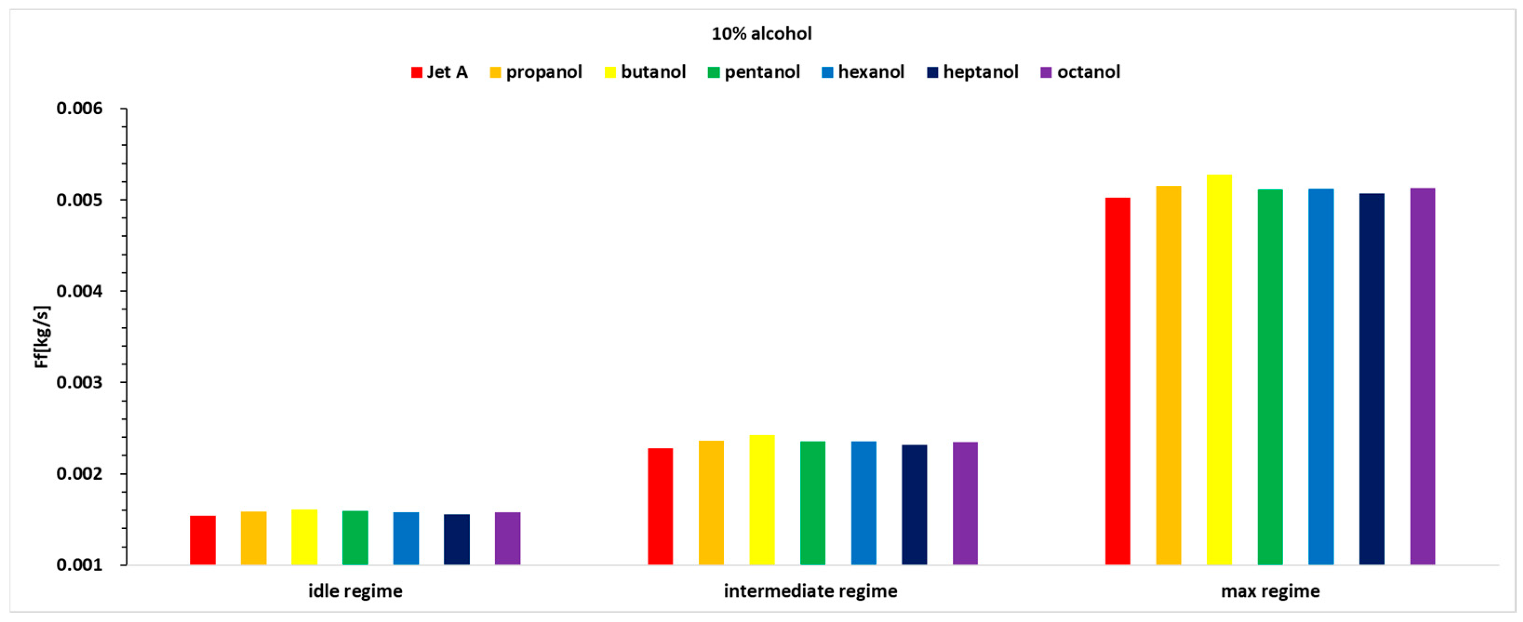
The exhaust gas temperature before the turbine is correlated with the fuel flow rate supplied by the fuel pump to the combustion chamber, as shown in Figure 6, Figure 7 and Figure 8. The analysis is based on mass flow rate, even though the engine instrumentation records volumetric flow rate. Using the determined densities for all tested fuels, the conversion from liters to kilograms was performed accurately.

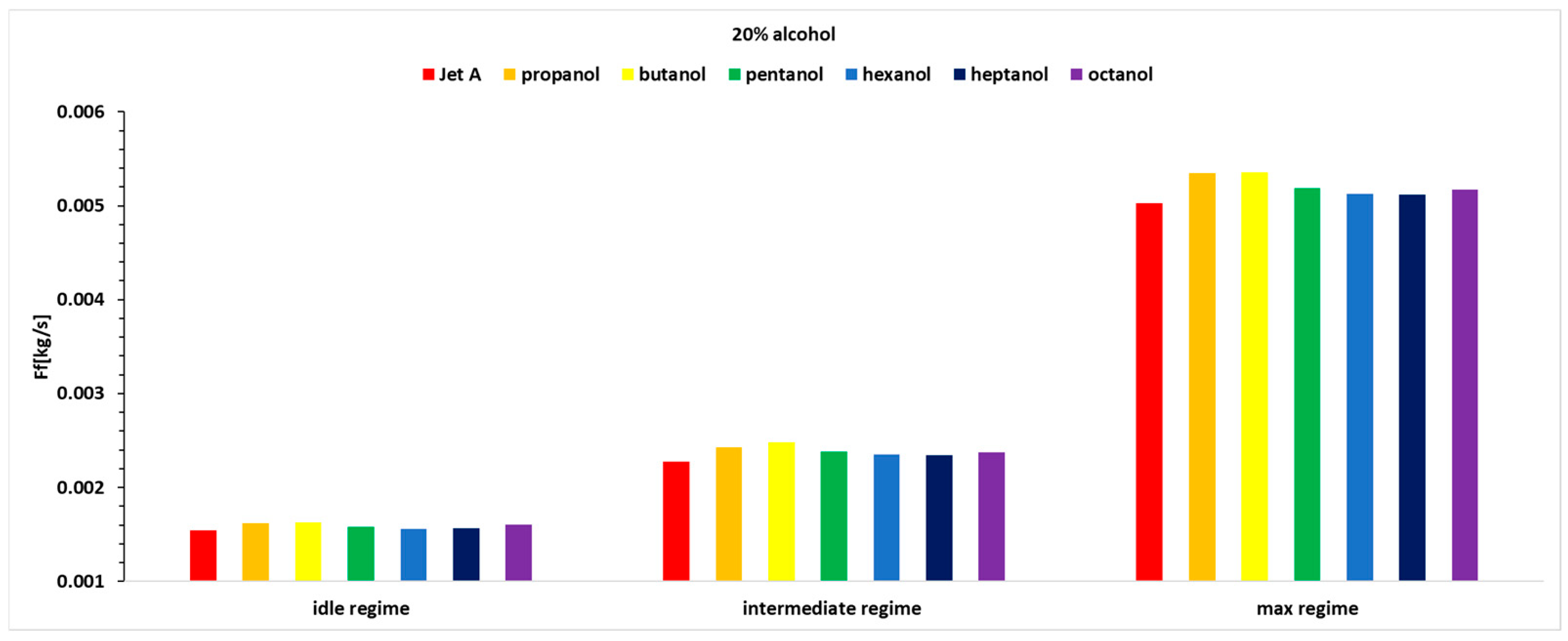
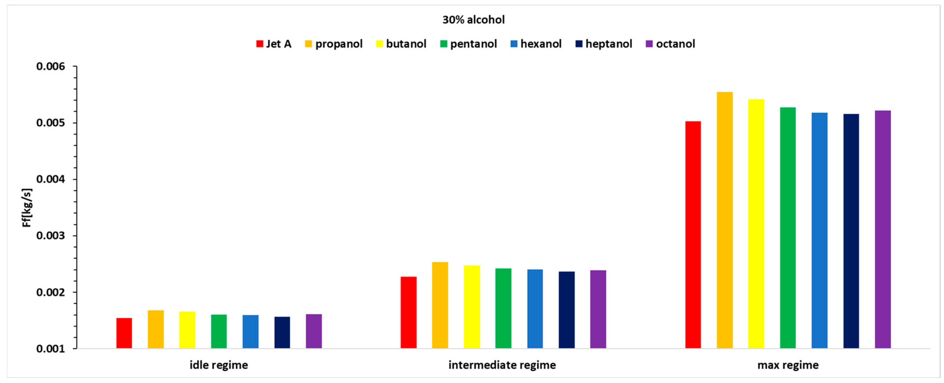
Analyzing Figure 6, Figure 7 and Figure 8, it can be observed that the fuel flow rate is higher in all cases where alcohol is added at the three analyzed concentrations of 10%, 20%, and 30%.

The fuel flow rate is higher for alcohols with lower carbon content, decreasing slightly when higher alcohols are used. As the exhaust gas temperature before the turbine decreases, the injected fuel flow rate increases.

A detailed analysis is presented in

Table 5. Percentage variation of the fuel mass flow rate for the three studied regimes and all analyzed fuels.

Percent [%]	Fuel	Propanol	Butanol	Pentanol	Hexanol	Heptanol	Octanol
	Regime	Variation [%]
10%	1	3.03	4.24	3.15	2.39	0.94	2.28
	2	3.77	6.35	3.40	3.40	1.91	3.17
	3	2.50	4.97	1.74	1.89	0.88	2.11
20%	1	4.93	5.55	2.77	1.15	1.81	4.25
	2	6.67	9.11	4.71	3.23	2.82	4.12
	3	6.45	6.62	3.26	2.04	1.89	2.89
30%	1	8.98	7.36	4.15	3.63	1.55	4.69
	2	11.30	8.65	6.42	5.46	3.93	5.08
	3	10.31	7.80	4.91	3.07	2.63	3.88

, showing the percentage variation of the fuel mass flow rate when using 10%, 20%, and 30% blends of the six alcohols for the three operating regimes analyzed. All of the tabulated data use as a reference baseline the fuel mass flow obtained while using Jet A alone. The results have been obtained by using an equation similar to Equation (8).

Analyzing the variation in fuel mass flow rate, it can be observed from Figure 6, Figure 7 and Figure 8 and Table 5 that there are variations of up to 11.3%, meaning the fuel mass flow rate increases by up to 11.3%.

For Regime 1, the fuel mass flow rate shows a decreasing curve for 10% and 20% alcohol concentrations added to Jet A, with maximum values observed for butanol. However, for the 30% alcohol concentration in regime 1, butanol no longer exhibits a maximum value.

In Regime 2, a similar trend to Regime 1 is observed.

In Regime 3, the maximum regime, the same trend as in Regimes 1 and 2 is observed. As the concentration of alcohol added to Jet A increases, the fuel flow rate percentage also increases.

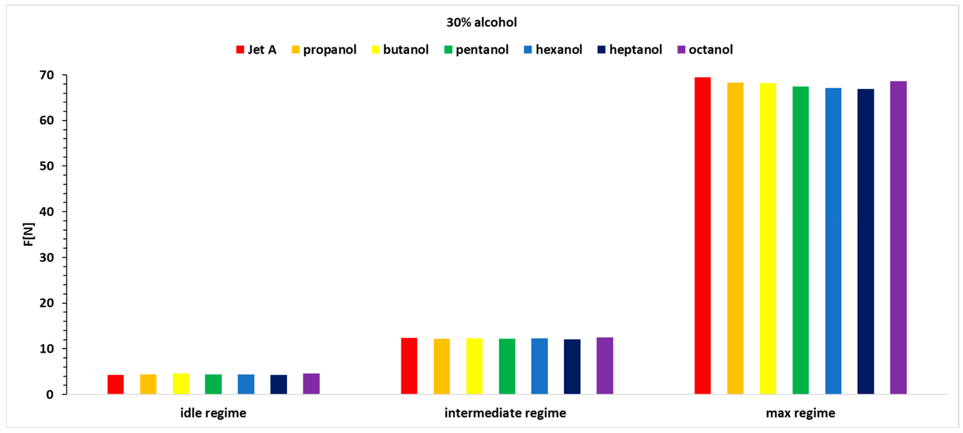
The exhaust gas temperature and the mass flow rate of fluid expelled through the reaction nozzle dictate the thrust produced.

Next, the thrust recorded by the micro-turbojet engine is analyzed in Figure 9, Figure 10 and Figure 11.

Even in cases where the exhaust gas temperature is lower than that of Jet A, the thrust is compensated by the fuel flow rate, as the higher density of the alcohols contributes to an increase in the total fluid flow rate.

A detailed analysis is provided in

Table 6. Percentage variation of thrust for the three operating regimes studied and all analyzed fuels.

Percent [%]	Fuel	Propanol	Butanol	Pentanol	Hexanol	Heptanol	Octanol
	Regime	Variation [%]
10%	1	1.73	0.84	−1.89	−0.91	−3.81	6.87
	2	−1.64	0.69	−2.68	−2.64	−4.92	−1.04
	3	−1.77	0.27	−2.22	−2.50	−3.95	−2.25
20%	1	3.07	6.19	0.94	2.69	0.40	1.86
	2	−1.62	1.77	−1.37	−1.60	−2.41	1.21
	3	−1.57	−0.87	−2.24	−3.28	−3.73	−3.13
30%	1	2.73	7.40	2.15	2.56	0.44	6.48
	2	−1.07	−0.80	−1.32	−0.88	−2.17	1.28
	3	−1.79	−1.82	−2.95	−3.46	−3.79	−1.27

, presenting the percentage variation of thrust when using 10%, 20%, and 30% blends of the six alcohols with Jet A for the three operating regimes analyzed. All the tabulated data use as a reference baseline the thrust obtained while using Jet A alone. The results have been obtained by using an equation similar to Equation (8).

Analyzing the variation in thrust, as shown in Figure 9, Figure 10 and Figure 11 and Table 6, reveals positive variations of up to 7.4% and negative variations of up to −4.92%.

In the first regime, which is more unstable, the percentage variation in thrust fluctuates for all three alcohol concentrations. However, octanol and butanol stand out with more significant increases in thrust.

Butanol and octanol exhibit the best performance across the three operating regimes and all three alcohol concentrations added to Jet A.

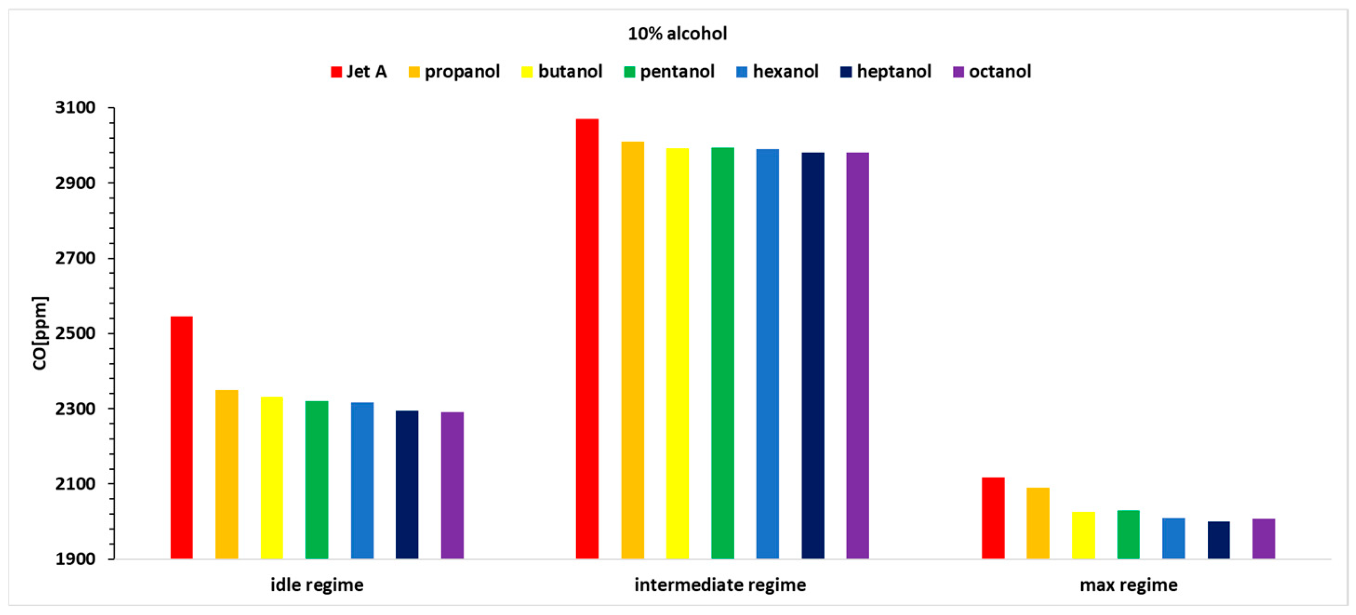
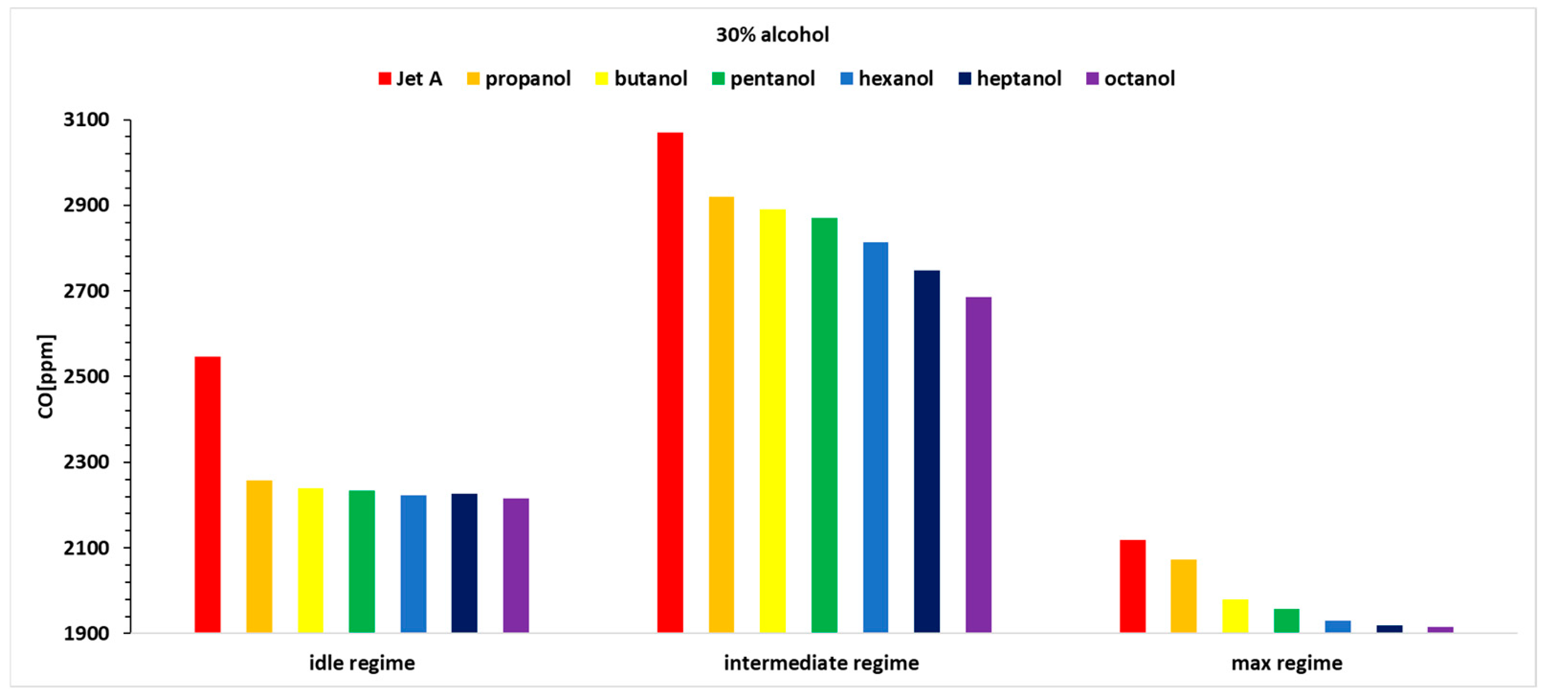
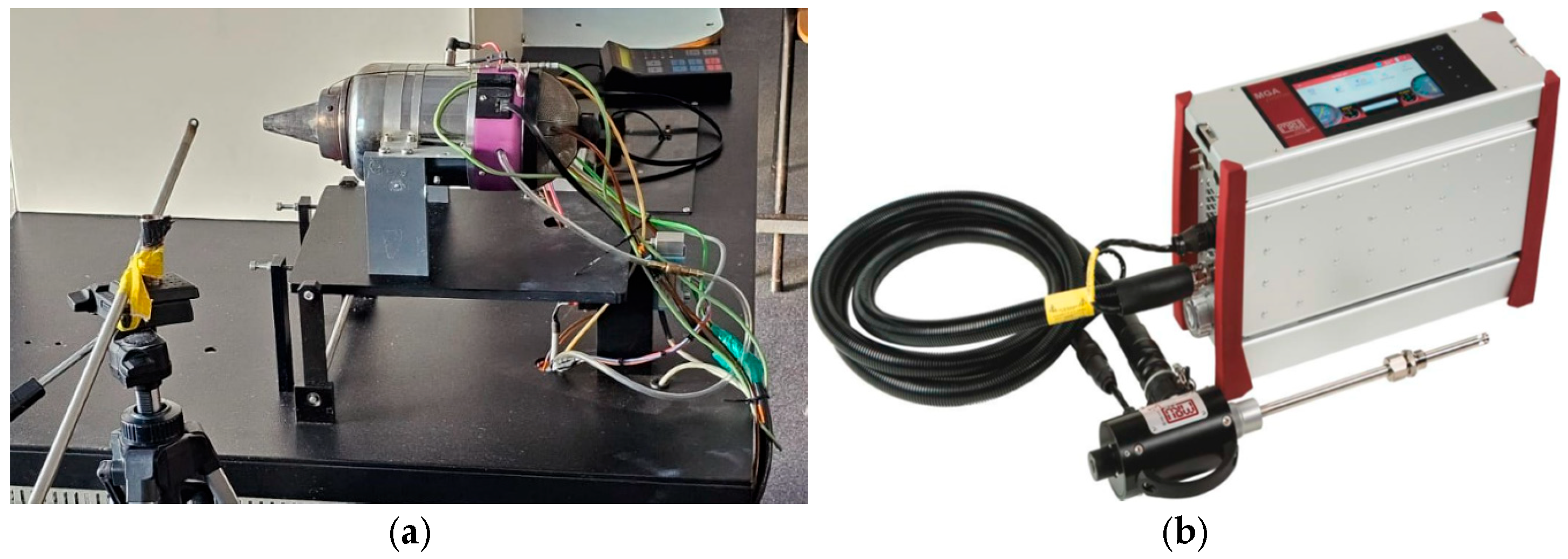
Hence, only the variation in CO concentration for the three operating regimes and the seven fuels is presented in Figure 12, Figure 13 and Figure 14. The CO sensor used on the analyzer is specially designed to eliminate the effects of hydrogen cross sensitivity (hydrogen compensated sensor). The sensor contains an extra electrode that allows the effect of sensitivity to hydrogen to be counteracted within the electronics. Thus, as well as the sensor being calibrated using a certified carbon monoxide test gas it is also calibrated using 1000 ppm of hydrogen. This ensures improved accuracy of the CO reading under all normal circumstances.

Analyzing the above figures, it can be observed that the CO concentration decreases across all three operating regimes as the carbon content in the alcohols increases.

A detailed analysis is presented in

Table 7. Percentage variation of CO concentration for the three operating regimes studied and all analyzed fuels.

Percent [%]	Fuel	Propanol	Butanol	Pentanol	Hexanol	Heptanol	Octanol
	Regime	Variation [%]
10%	1	−7.70	−8.41	−8.88	−9.03	−9.86	−9.98
	2	−1.95	−2.54	−2.48	−2.61	−2.90	−2.93
	3	−1.32	−4.39	−4.15	−5.10	−5.57	−5.24
20%	1	−8.76	−10.64	−11.43	−12.25	−12.33	−12.88
	2	−2.28	−2.44	−4.30	−4.72	−6.38	−9.77
	3	−1.79	−2.93	−6.47	−7.18	−7.93	−8.88
30%	1	−11.31	−12.02	−12.25	−12.73	−12.57	−12.96
	2	−4.89	−5.86	−6.51	−8.37	−10.52	−12.51
	3	−2.17	−6.52	−7.60	−8.88	−9.35	−9.58

, showing the percentage variation of CO concentration when using 10%, 20%, and 30% blends of the six alcohols for the three analyzed regimes. All the tabulated data use as a reference baseline the CO emissions obtained while using Jet A alone. The results have been obtained by using an equation similar to Equation (8).

It can be observed that the percentage variation of CO concentration, relative to the baseline case for Jet A, shows values lower by up to nearly 13%.

A trend of decreasing concentration can be noticed as the carbon content in the alcohol molecule increases. Thus, the best alcohol in terms of CO concentration is octanol.

3.4. Micro-Turbojet Performance Results

Based on the measurements recorded by the micro-turbojet instrumentation, several important engine performance parameters can be calculated.

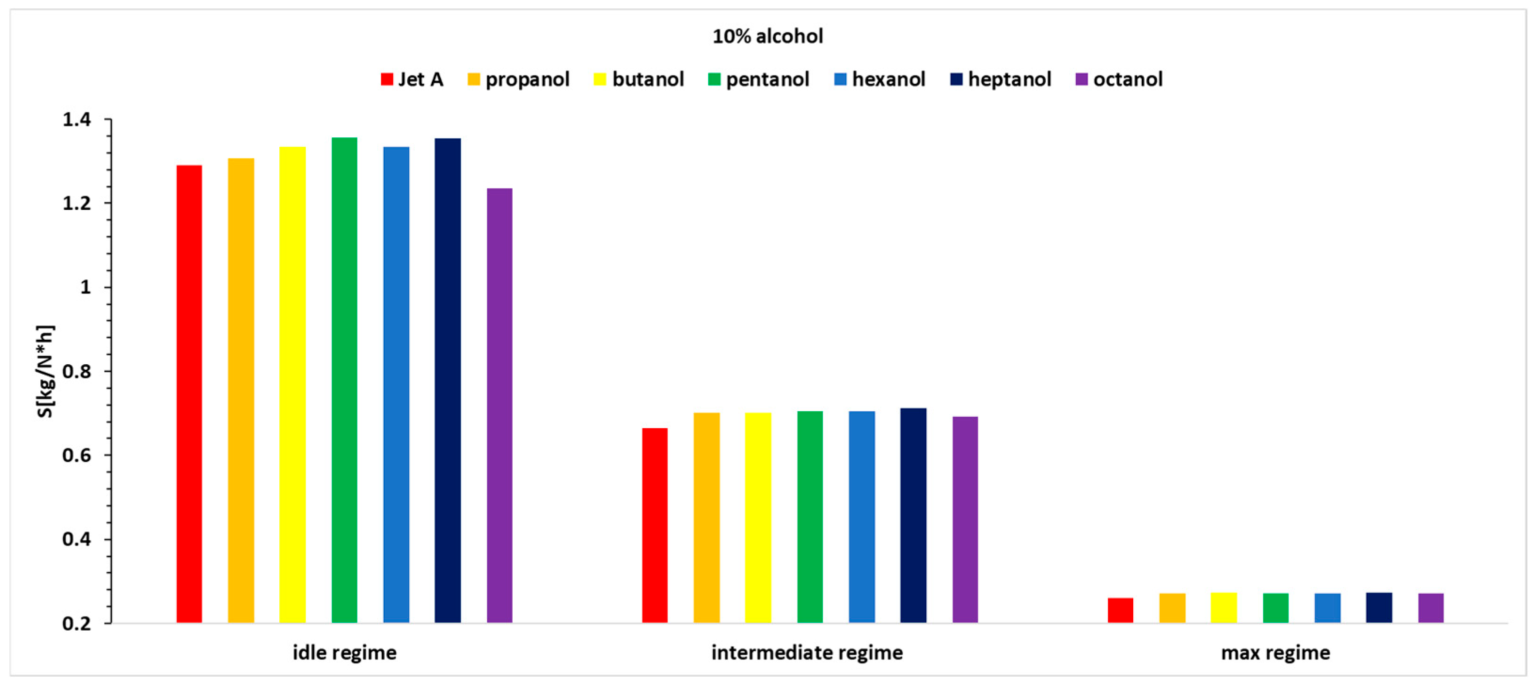
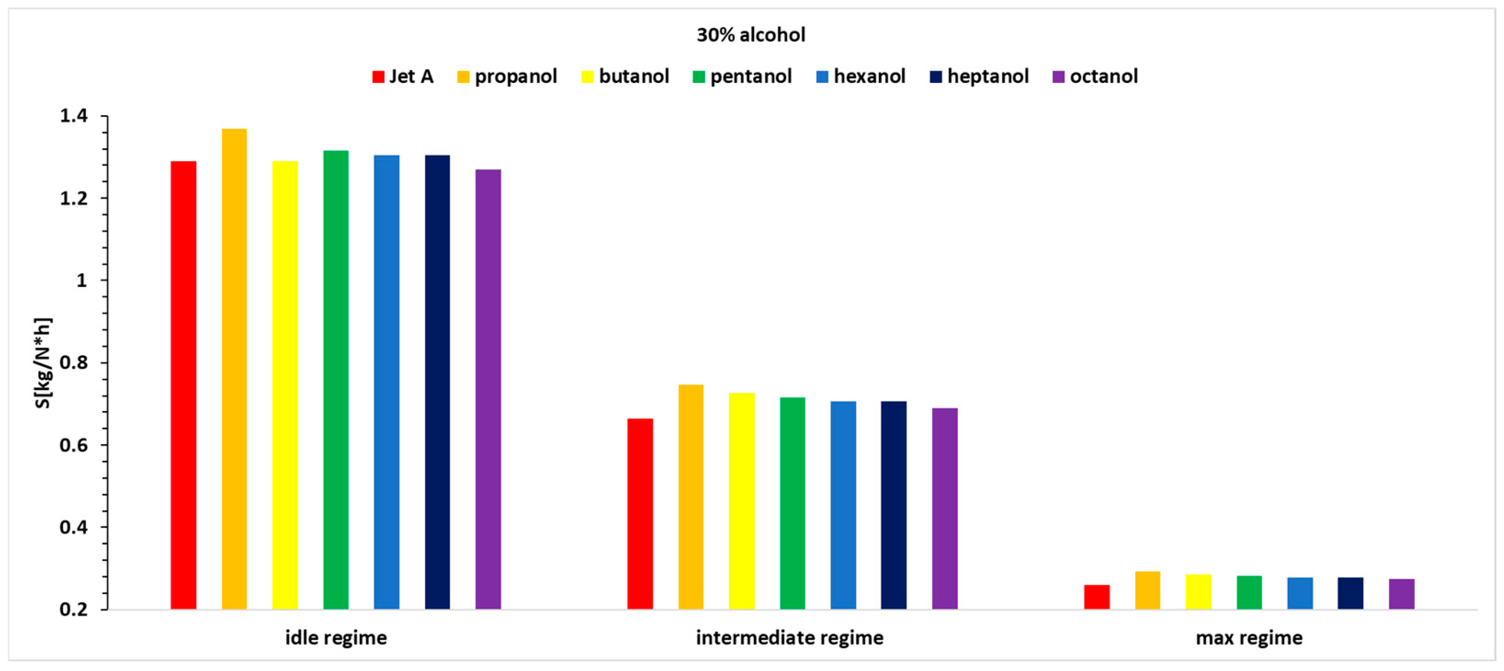
One of the most important parameters for turbomachinery is the specific fuel consumption, according to Formula (5), which combines fuel consumption and the thrust produced by the micro-turbojet into a single value.

Figure 15, Figure 16 and Figure 17 present the variation in specific fuel consumption for the three studied regimes (1 being idle, 2 being intermediate and 3 being max), for the seven fuels at the three alcohol concentrations used.

Analyzing Figure 15, Figure 16 and Figure 17, it can be observed that the idle regime, as known, is a more unstable regime compared with the other operating regimes. It does not show a clear trend of increase or decrease as the carbon concentration in the alcohols increases, but the variations are not significant. In the second regime, a higher specific fuel consumption is observed when using alcohol blends, and this increases with the alcohol concentration, which is expected because the calorific value of alcohols is lower than that of Jet A. The specific fuel consumption is highest for propanol, gradually decreasing to octanol, which shows the smallest increase compared with the specific fuel consumption when using Jet A. A detailed analysis is presented in

Table 8. Percentage variation of specific fuel consumption for the 3 studied regimes and all analyzed fuels.

Percent [%]	Fuel	Propanol	Butanol	Pentanol	Hexanol	Heptanol	Octanol
	Regime	Variation [%]
10%	1	1.28	3.37	5.13	3.32	4.94	−4.30
	2	5.51	5.62	6.25	6.20	7.18	4.25
	3	4.35	4.69	4.05	4.50	5.03	4.46
20%	1	1.81	−0.60	1.82	−1.50	1.41	2.35
	2	8.43	7.21	6.16	4.91	5.35	2.88
	3	8.16	7.55	5.62	5.50	5.84	6.21
30%	1	6.08	−0.04	1.96	1.04	1.11	−1.67
	2	12.51	9.52	7.85	6.39	6.24	3.76
	3	12.32	9.80	8.10	6.76	6.67	5.22

, showing the percentage variation of specific fuel consumption when using 10%, 20%, and 30% blends of the six alcohols for the three regimes studied. All of the tabulated data use as a reference baseline the specific fuel consumption obtained while using Jet A alone. The results have been obtained by using an equation similar to Equation (8).

Regarding the specific fuel consumption, it can be observed that for regime 1, which is a more unstable regime, no specific variation trend is apparent. However, octanol shows advantages at a 10% concentration, while butanol shows advantages at a 20% concentration, and both butanol and octanol show advantages at a 30% concentration.

For regime 2, a decreasing trend in specific fuel consumption can be observed from propanol to octanol when using 20% and 30% alcohol in the blend. In the case of regime 2 and 10% alcohol, the trend is increasing from propanol to heptanol.

For Regime 3, a similar decreasing trend in specific fuel consumption is observed from propanol to octanol when using 20% and 30% alcohol in the blend. In the case of Regime 3 and 10% alcohol, the variations do not present any specific trend.

Therefore, adding 10% alcohol does not present a clear picture in terms of specific fuel consumption variations. When using 20% and 30% alcohol, in Regimes 2 and 3, the trends are clear, showing a decreasing variation from propanol to octanol.

In

Table 9. Recorded values for $T_{\_comp}$ and $\dot{M}a$ for Regime 3.

Jet A	Percent	Propanol	Butanol	Pentanol	Hexanol	Heptanol	Octanol
${\mathrm{T}}_{\_\mathrm{comp}}$ [°C]
121.0	10%	117.9	118.4	118.8	119.9	121.1	121.6
	20%	118.0	118.3	118.5	119.4	121.8	119.6
	30%	118.2	118.9	119.0	119.5	121.5	118.9
$\dot{\mathrm{M}}\mathrm{a}$ [kg/s]
0.226	10%	0.222	0.224	0.223	0.223	0.223	0.225
	20%	0.223	0.224	0.224	0.224	0.223	0.225
	30%	0.224	0.225	0.225	0.224	0.224	0.226

, the compressor outlet temperature and the air mass flow rate recorded by the micro-turbine instrumentation at Regime 3 are presented, as these are the parameters involved in Equations (7) and (8), which are used to generate the data shown in Figure 18 and Table 9.

It can be observed that the variations in temperature for the blends are relatively small (ranging from 117.9 °C to 121.6 °C) and fall within the error margin of the type K thermocouples used (±1.1 °C), indicating good thermal stability of the system. In the case of certain blends, such as 10% propanol or 20–30% octanol, a slight decrease in the compressor outlet temperature is observed, without affecting the proper functioning of the engine. This decrease may be attributed to changes in the air–fuel mixture density but does not significantly influence the compressor efficiency. Regarding the airflow rate, the values obtained (between 0.222 and 0.225 kg/s) indicate stable operation of the compressor–combustion chamber assembly, with no major deviations induced by the type of fuel used. This consistency confirms the good compatibility of the blends with the tested engine and supports their use without the need to recalibrate the air supply system.

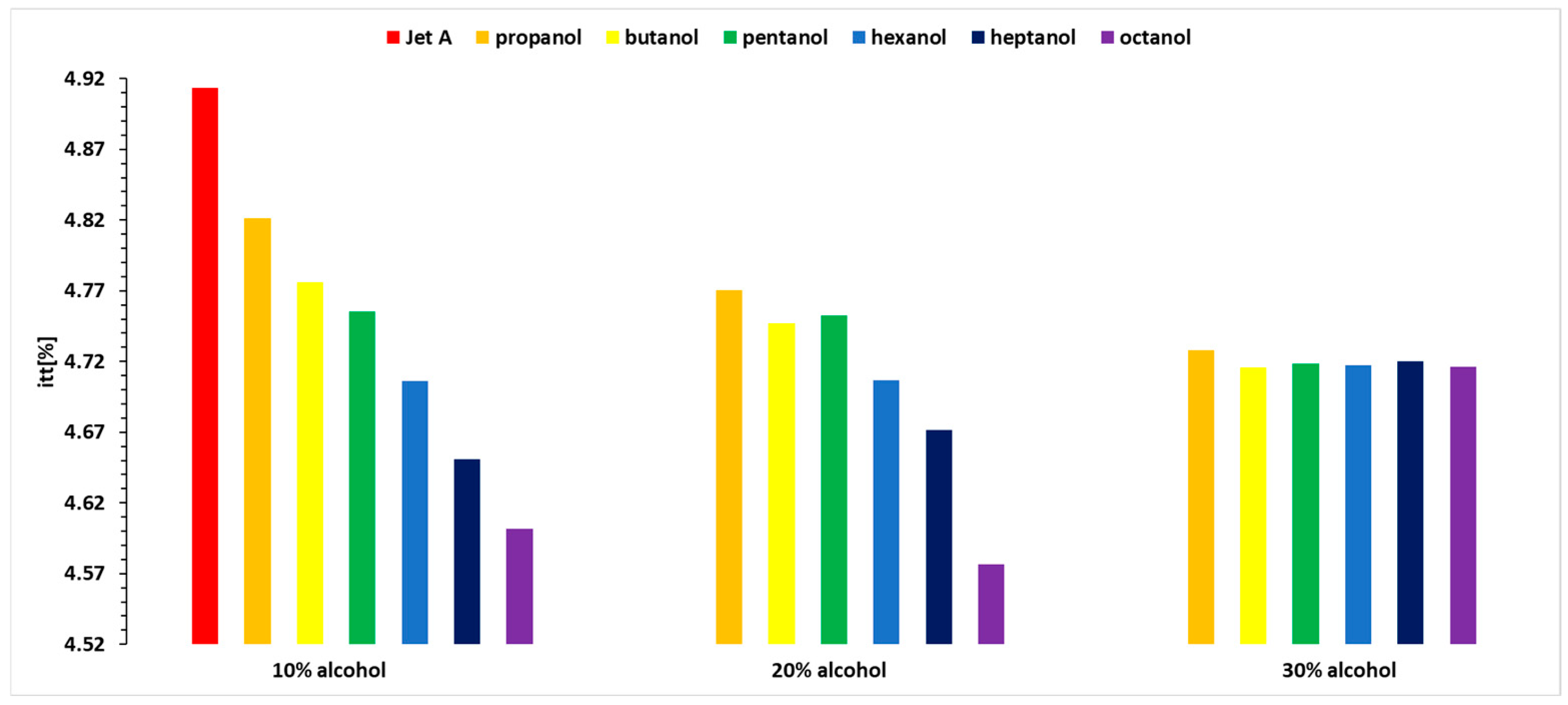
Another important parameter, according to Equation (7), is the engine’s thermal efficiency. Figure 18 shows the variation in thermal efficiency for the maximum regime when using 10%, 20%, and 30% alcohol in the fuel blends.

By analyzing Figure 18, it can be observed that the thermal efficiency in the maximum regime decreases with the increase in alcohol concentration. According to Equation (7), this combination of propulsive force, exhaust gas flow, and calorific power causes the thermal efficiency to exhibit small variations.

Another parameter that can be analyzed, according to Equation (6), is the combustion efficiency in the combustion chamber. Thus, the most indicative results are for the maximum regime.

By analyzing

Table 10. Variation in combustion efficiency at maximum regime for all tested fuels.

Jet A	Alcohol %	Propanol	Butanol	Pentanol	Hexanol	Heptanol	Octanol
ηb [%]
85.28	10	85.35	84.62	85.46	84.71	84.34	85.82
	20	84.44	84.39	87.31	86.90	85.86	86.90
	30	84.07	85.59	86.58	86.80	85.70	87.20

, it can be observed that the combustion efficiency shows small variations around the value obtained for Jet A, which is 85.28%, with variations of up to ±2%.

The errors associated with the parameters in Equation (6) must be considered in order to evaluate the significance of the variations observed between the different blends. The type K thermocouples used for temperature measurements have a typical uncertainty of ±1.1 °C, which introduces a possible variation in the calculation of the enthalpy difference (the terms involving T_comb and T_comp). Regarding the mass flow rates, the flow sensors have an estimated uncertainty of ±1–2%, directly affecting the $\dot{M}a$ and $\dot{M}f$ terms. The specific heat capacities (cp) are determined based on temperature and may introduce an additional error of ±1% in the calculation. Moreover, the lower calorific value (LCP) of each fuel blend naturally varies depending on the alcohol type and concentration; however, these values were considered constant and were taken from bibliographic sources. Therefore, the overall propagated error in the calculation of η_b can be estimated at approximately ±1.5%. This value must be considered when interpreting the differences in combustion efficiencies among the blends—for example, differences below 1% between propanol and Jet A fall within this uncertainty range and cannot be considered statistically significant. In contrast, the larger differences (over 2%) observed for blends with pentanol, heptanol, or octanol suggest a possible real thermodynamic advantage, but one that requires confirmation through repeated testing and further experimental validation.

Similar values to those presented in this study were also obtained in [13,14], with some differences that are mainly due to varying atmospheric conditions, as the experiments were conducted on different days. It is well known that ambient temperature and pressure significantly influence the values recorded during testing. Other bibliographic sources [16,17,18,19] also report similar findings regarding the variation of key parameters, consistent with those observed in this study. However, the tests in those studies were performed on different types of gas turbine engines.

4. Conclusions

The analysis of the results from the various operating regimes reveals several important trends and insights into the impact of alcohol blends on micro-turbojet engine performance, combustion efficiency, and emissions.

It was observed that the amount of CO₂ produced during stoichiometric combustion decreased as the carbon percentage in the alcohol blend decreased. Among the alcohols tested, octanol produced the highest CO₂ emissions due to its higher carbon content. In contrast, propanol, with a lower carbon content, emerged as the most suitable alcohol in terms of CO₂ emissions. However, it also exhibited the lowest calorific value, which influenced its engine performance.

The exhaust gas temperature, measured before the turbine, was generally lower for alcohol blends than for the baseline Jet A fuel in the first two operating regimes, indicating a lower combustion temperature due to the reduced calorific value of alcohols. In the third regime (maximum regime), however, the exhaust temperature increased slightly as the carbon content in the alcohols increased. Specifically, butanol and higher alcohols resulted in higher exhaust gas temperatures, while propanol showed a decrease.

The fuel mass flow rate was observed to increase with the addition of alcohols at all concentrations (10%, 20%, 30%). This increase was more pronounced with alcohols with a lower carbon content. The fuel flow rate was highest for alcohols like propanol and decreased slightly as the alcohol chain length increased (e.g., butanol, octanol). This suggests that higher alcohols require more fuel to achieve similar levels of combustion efficiency compared with lower alcohols.

The variation in thrust was relatively small, with positive variations of up to 7.4% and negative variations up to −4.92%. However, alcohols like butanol and octanol showed more significant increases in thrust, particularly in the first operating regime, where the system was more unstable. In general, alcohols with a higher carbon content (e.g., butanol and octanol) showed better performance in terms of thrust production, despite minor fluctuations in specific regimes.

The concentration of CO in the exhaust gases was found to decrease as the carbon content of the alcohols increased, indicating more efficient combustion. Octanol produced the lowest CO concentration, signifying its better combustion efficiency among the alcohols tested.

Specific fuel consumption was highest for propanol, reflecting its lower calorific value. As alcohol chain length increased, specific fuel consumption decreased, with octanol showing the lowest increase in specific fuel consumption when compared with Jet A. For regimes with 20% and 30% alcohol, the specific fuel consumption showed a decreasing trend from propanol to octanol.

Thermal efficiency in the maximum regime decreased with the increase in alcohol concentration. This was due to the lower calorific value of alcohols, which caused small variations in thermal efficiency. Despite these decreases, alcohol blends still demonstrated relatively efficient thermal behavior compared with the baseline Jet A fuel.

Combustion efficiency, calculated for the maximum regime, exhibited small variations around the baseline value of 85.28% for Jet A, with variations of up to ±2%. This suggests that the addition of alcohols did not significantly affect the combustion efficiency in the combustion chamber, maintaining a similar level of efficiency to Jet A.

The results suggest that alcohols, particularly butanol and octanol, offer promising alternatives to Jet A fuel, especially in terms of emissions reductions (e.g., CO₂ and CO). However, the trade-off in performance, particularly regarding fuel consumption and thermal efficiency, needs to be considered carefully. While alcohols with lower carbon content (such as propanol) are more environmentally friendly in terms of CO₂ emissions, they also exhibit poorer engine performance due to their lower calorific value. For optimal performance, a balance between emissions and fuel efficiency must be achieved, and higher alcohols like butanol and octanol seem to offer the best overall performance across various operating regimes.

Future works will be performed and gaseous pollution will be taken into account (e.g., NO_x, HC, etc.) in order to assess the environmental impact of using such blends in an aviation engine.