Simulation Study and Proper Orthogonal Decomposition Analysis of Buoyant Flame Dynamics and Heat Transfer of Wind-Aided Fires Spreading on Sloped Terrain

Abstract

The wind and slope are deemed to be the determinant factors driving the extreme or erratic spread behavior of wildfire, which, however, has not been fully investigated, especially to elaborate the mechanism of fire spread associated with heat transfer and fluid dynamics. A systematic study is therefore carried out based on a physical-based simulation and proper orthogonal decomposition (POD) analysis. Results show that compared to the wind, the slope plays a more profound effect on the fire structure; with the increase in slope, the fire line undergoes a transition from a W-shape to the U- and pointed V-shape, accompanied by stripe burning zones, indicating a faster spread but incomplete combustion. The wind effect is distinguished by mainly inducing a turbulent backflow ahead of the fire front, while the slope effect promotes convective heating via the enhanced slant fire plume. Different mechanisms are also identified for the heat transfer ahead of the fire line, i.e., the radiative heat is affected by the combined effects of the flame length and view angle, and in contrast, the convective part of the heating flux is dominated by the action of the flame attachment, which is demonstrated to play a crucial role for the fire spread acceleration at higher slopes (>20°). The POD analysis shows the distinct pattern of flame pulsating for the respective wind and slope effects, which sheds light on modeling the unsteady features of fire spreading and reconfirms the necessity of considering the different effects of these two environmental factors.

1. Introduction

Wildfire activity has increasingly been reported in recent years [1], causing catastrophic damage biologically or ecologically [2] and posing unprecedented fire threat to communities near the wildlands–urban interface [3], whose study therefore becomes imperative with a focus on the fire spreading mechanism. Wildfire is a very complex phenomenon, involving highly nonlinear interactions between fire dynamics, vegetation chemistry, and environmental conditions (wind, humidity, rough terrain, etc.) [4,5]. To predict reliably a fire’s behavior and spread for emergency response and mitigation of forest fire risks, a further understanding of the basic influential elements that are responsible for the extreme or erratic fire spreading is necessary.

Wind is commonly accepted to be important to the dynamic processes of wildfire initiation and spreading. During the fire–atmosphere interactions, the wind effect is usually determined by two components, i.e., atmospheric wind and fire-induced wind. A field experiment conducted by Clements and Seto [6] showed that the fire-induced circulation was formed because of the ambient shear and thermal instability related to the sensible heat flux from the fire. The strong fire-induced wind was responsible for the enhanced turbulence’s kinetic energy and a minimum in atmospheric pressure. The spectral analysis of the measured velocity field during the fire-front passage indicated that the increased energy in velocity and temperature spectra at high frequency was caused by the dynamics of small eddies near the fire plume [7]. Kochanski et al. [8] suggested that with a strong vertical shear in the ambient wind field, the fire may develop an erratic behavior. The role of the coupling between fire and fire-induced flow was also demonstrated in the numerical simulations by Sun et al. [9] They found that the head fire’s rate of spread (ROS) and area burned were substantially enhanced, as much as doubled, when the fire–atmosphere coupling was considered. However, a more reliable simulation is required to further understand the physics underlying a fire’s acceleration, since in the work of Sun et al. [9], the fire’s sensible flux was coupled to the atmosphere in an empirical way. Additionally, since extreme wildfires usually occur on complex terrains [1,10,11], those wind effects also need to be quantified together with the slope effect to fully untangle the extreme fire dynamics under the real environmental conditions [12].

For the slope effect, based on a laboratory-scale experiment, Dupuy et al. [13] reported that the increase in slope could greatly increase the ROS, and it was hypothesized to be related to the stronger fire-induced wind in high-slope conditions. Silvani et al. [14] further observed the appearance of fire whirls rolling along the flank of the fire front under a steeper slope. The author then stressed the importance of fluid dynamics to explain the remarkable change in fire spread rate. Meanwhile, a combined radiative–convective heating mode was deemed to dominate the heat transfer and thus the fire spread when the slope was increased [15]. However, as indicated by the experimental results of Xie et al. [16], for a steeper slope, there is an increased likelihood of flame attachment and therefore, the convective heating seems to be the mechanism explaining the fire acceleration.

The ambiguous conclusion on the main heating mode over the unburned vegetation may be because the convective energy transfer is difficult to measure in an experiment [17], but a more quantitative examination of the heat transport is necessary to accurately evaluate the wind and slope effects. For most fire spread models of operational use, for example, the Rothermel model [18], an analogy has often been invoked between wind and slope effects; an effective wind speed was explicitly incorporated to account for the slope terrains based on the assumption that the fire spread mainly resulted from the increase in incident radiation [19]. However, this limits the applicability of most empirically derived fire models for predicting the extreme fire spread under complex environment conditions [13,20].

Given these limitations of existing models and the challenges in experimental investigations, it becomes evident that a deeper understanding of the fundamental mechanisms governing fire spreading, particularly those related to heat transfer and fluid dynamics, is crucial. In recent years, with the advancement of numerical methods, the computational fluid dynamics (CFD)-based analysis of wildfire spread has gained great attention. Mell et al. [21] conducted a pioneer work to study grassland fires using the physics-based model of WFDS (wildlands–urban interface fire dynamics simulator), which showed a favorable capability in physically predicting fire properties compared to semi-empirical or empirical models. Adopting the WFDS model, Sánchez-Monroy et al. [22] investigated the upslope fire spread for fuel beds at various slopes to compare the spread of fire on different slopes. The simulations reproduced the experimental trend and identified the convection-dominated regime as the slope ranging from 30° to 45°. However, in those cases, the effect of wind speed was still unknown. Moinuddin et al. [23] discussed the wind effect alone and revealed a linear relationship between ROS and wind speed in the considered cases. Furthermore, for now, the fluid dynamics associated with the changes in spread mode (e.g., flame spread acceleration) that were indicated in previous experiments have not been fully investigated.

Another advantage of physics-based modeling that should be noticed is the large quantity of meaningful flow data. Processing these data based on data-driven strategies can be helpful in revealing the coherent motion that governs erratic fire behavior and extracting meaningful insights. One of the most popular data-driven fluid analysis methods is the proper orthogonal decomposition (POD) [24]. Mathematically, the POD is a decomposition technique that determines a set of orthogonal basis or mode functions for given input data (or the target field variables), $X(x,t)$; these basis functions are identified as the optimal candidates for collectively expressing the original data. The critical features of turbulent flow, for example, can then be efficiently captured through the combination of the basis functions that represent the most energetic flow structures. This method has therefore been often applied to examine the dominant fluctuating and coherent structures within the various types of fluid flow [25].

Kostas et al. [26] utilized POD to analyze the instantaneous velocity field and vorticity field of flow over a backward-facing step, while Podvin et al. [27] established a connection between the first few high-energy POD modes and the shear layer’s instability in the cavity flow. The POD analysis was also successfully applied to understand the flow–flame interactions, such as by Shen et al. [28], where the POD identified the different interaction modes between the precessing vortex core and the swirling flame under different inlet fuel conditions. A POD analysis of an instantaneous OH field and velocity-temperature field also revealed the locations of ignition kernels and flame growth for the flames stabilized in the hot-coflow configuration [29]. For wildfires, Guelpa et al. [30] once used a POD for model order reduction in order to improve the computational efficiency of physical models solving the wildfire behavior. However, to the best of our knowledge, there has been no attempt yet to understand the coherent structures that govern the fire-induced flow and heat transport with a POD.

Therefore, this study aims to systematically investigate the characteristics of fire spread under various wind and slope effects, and a focus is given to the understanding of the mechanism underlying fire erratic behavior. This is achieved by performing a detailed parametric study and a quantitative analysis of the fluid mechanics and heat transfer based on physics-based numerical simulations [31]. The modal analysis, facilitated by a proper orthogonal decomposition, is also employed for the first time to examine the coherent structures that govern the propagating flame front in wildfires.

2. Computational Methods

A multiphase formulation of mass, momentum, and energy equations was considered for the present wildfire simulation to account for phase coupling during the fire spread on solid vegetation. The thermally driven gas flow was solved by a low-Mach number LES approach based on the open source code of Fire Dynamics Simulator (FDS 6.7.7) [31]. Combustion in gas flow was modeled using the Eddy Dissipation Concept (EDC), and the radiation, as the main driving mechanism for fire spreading, was solved by the finite-volume method [31].

2.1. Gas-Phase Governing Equations

Considering the gas–solid interactions, the fluid conservation equations for mass ($\rho$), momentum ($\mathbf{u}$), species ($Z_{\alpha }$), and sensible energy ($h_s$) are given by

$${\displaystyle \frac{\partial \rho }{\partial t}}+\nabla ·\left(\rho \mathbf{u}\right)={\dot{m}}_b^{″}$$

(1)

$${\displaystyle \frac{\partial \mathbf{u}}{\partial t}}-\mathbf{u}\times \omega +\nabla H-\tilde{p}\nabla \left({\displaystyle \frac{1}{\rho }}\right)={\displaystyle \frac{1}{\rho }}\left[(\rho -{\rho }_0)\mathbf{g}+{\mathbf{f}}_{\mathrm{b}}+\nabla ·\tau \right]$$

(2)

$${\displaystyle \frac{\partial }{\partial t}}\left(\rho Z_{\alpha }\right)+\nabla ·\left(\rho Z_{\alpha }\mathbf{u}\right)=\nabla ·(\rho D_{\alpha }\nabla Z_{\alpha })+{\dot{m}}_{\alpha }^{‴}+{\dot{m}}_{b,\alpha }^{‴}$$

(3)

$${\displaystyle \frac{\partial }{\partial t}}\left(\rho h_s\right)+\nabla ·\left(\rho h_s\mathbf{u}\right)={\displaystyle \frac{D\overline{p}}{Dt}}+{\dot{q}}^{‴}+{\dot{q}}_b^{‴}+\nabla ·{\dot{\mathbf{q}}}^{″}$$

(4)

where $\rho$ is the gas density, $\mathbf{u}$ is the velocity vector, $\tau$ is the viscous stress, the term ${\mathbf{f}}_{\mathrm{b}}$ represents the drag force exerted by fuel particles, $\omega$ is the vorticity vector, $\tilde{p}$ the pressure perturbation, $D_{\alpha }$ the species’ diffusion coefficients. ${\dot{m}}_b^{″}$ and ${\dot{m}}_{b,\alpha }^{‴}$ are the mass increment due to particle degradation, and ${\dot{m}}_{\alpha }^{‴}$ stems from the chemical reactions. ${\dot{q}}^{‴}$ is the heat release rate, ${\dot{q}}_b^{‴}$ denotes the energy transferred to particles, and ${\dot{\mathbf{q}}}^{″}$ accounts for the subgrid heat fluxes of conduction and radiation. $H={\left|\mathbf{u}\right|}^2/2+\tilde{p}/\rho$ is the stagnation energy per unit mass.

Equation (1) describes the conservation of mass in the grid; Equation (2) is the conservation of momentum equation, which considers the buoyancy effect caused by density difference, the drag effect of particles, and the effect of viscous force; Equation (3) is the component conservation equation for different components Z, and Equation (4) is a simplified energy equation for low Mach numbers.

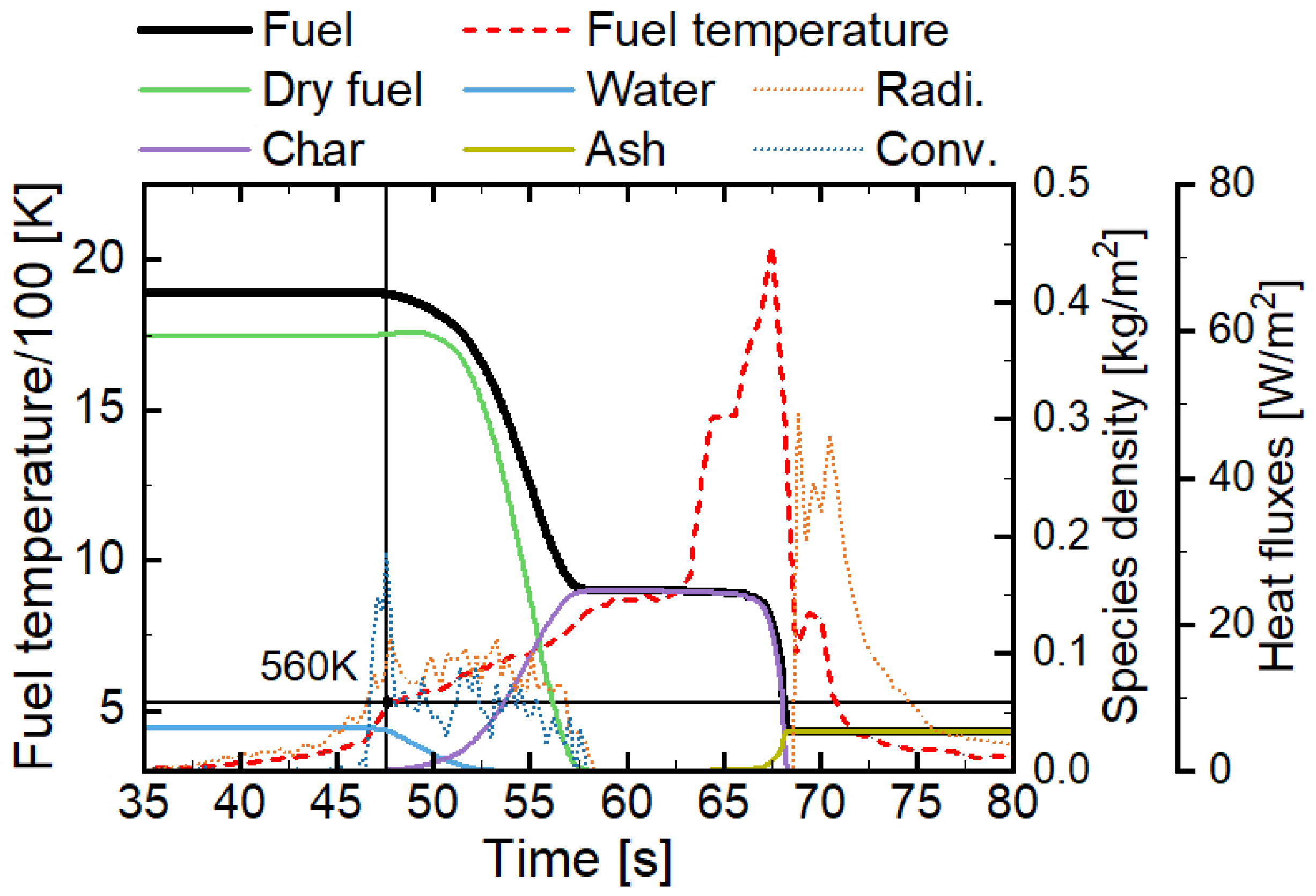
2.2. Vegetation Fuel Model

In a wildfire, the fire spread is controlled by the close interplay between the combined slope and wind actions and the solid fuel (vegetation) combustion [32]. Therefore, considering vegetative fuel is usually composed of fine particles, the fuel element (FE) model was employed, which represents the vegetation as thermally thin fuel particles that are inserted within each numerical grid with assigned physiochemical properties. Compared to the alternative model available in FDS, i.e., the boundary fuel (BF) model, theoretically, the FE model can more reliably solve the fuel thermal-degradation process affected by both the convective and radiant heat transfers [31] that are one of the primary focus in this study; contrarily, the BF model assumes the fuel burns like a porous solid and in a radiation-dominated mode.

Therefore, a three-step thermal degradation was considered to model complex fuel pyrolysis and its interaction with the air flow. It included three successive reactions, i.e., the water evaporation and then the pyrolysis of dry vegetation, which are both endothermic, followed by the exothermic char oxidation:

Drying:

$$\mathrm{Vegetation}\Rightarrow {\gamma }_{{\mathrm{H}}_2\mathrm{O}}{\mathrm{H}}_2\mathrm{O}+(1-{\gamma }_{{\mathrm{H}}_2\mathrm{O}})\mathrm{Dry}\mathrm{Vegetation}$$

(5)

Pyrolysis:

$$\mathrm{Dry}\mathrm{Vegetation}\Rightarrow {\gamma }_{\mathrm{char}}\mathrm{Char}+(1-{\gamma }_{\mathrm{char}})\mathrm{Fuel}\mathrm{Gas}$$

(6)

Char oxidation:

$$\mathrm{Char}+{\gamma }_{\mathrm{char},{\mathrm{O}}_2}{\mathrm{O}}_2\Rightarrow (1+{\gamma }_{\mathrm{char},{\mathrm{O}}_2}-{\gamma }_{\mathrm{ash}}){\mathrm{CO}}_2+{\gamma }_{\mathrm{ash}}\mathrm{Ash}$$

(7)

where the stoichiometric constant ${\gamma }_{{\mathrm{H}}_2\mathrm{O}}=M/(1+M)$, and M is the fuel moisture content determined based on a dry weight. ${\gamma }_{\mathrm{char}}$ is the mass fraction of dry fuel decomposed into char, and ${\gamma }_{\mathrm{ash}}$ is the mass fraction of char that is converted to ash during the oxidation process. ${\gamma }_{\mathrm{char},{\mathrm{O}}_2}=1.65$ is the oxygen consumption coefficient [33]. The above three-step degradation of solid was solved like the element reactions in the gas phase, then, to calculate the mass generation rate of the product in each reactions, the Arrhenius type kinetics were used. The formula is as follows:

$${\displaystyle \frac{d{m}_f}{dt}}=-k\prod C_{\alpha }$$

(8)

$$k=AT{e}^{{\displaystyle \frac{-E_a}{RT}}}$$

(9)

where $m_f$ is the fuel mass, $C_{\alpha }$ is the concentration of fuel, A is the pre-exponential factor, $E_a$ is the activation energy, R is the universal gas constant, and T is the temperature.

Associated with the mass change, the variation in solid vegetation temperature ($T_{\mathrm{s}}$) was modeled as follows:

$${\rho }_{\mathrm{b}}{c}_{\mathrm{p},\mathrm{b}}{\displaystyle \frac{d{T}_{\mathrm{s}}}{dt}}=-{\dot{Q}}_{\mathrm{s}.\mathrm{vap}}^{″}-{\dot{Q}}_{\mathrm{s}.\mathrm{kin}}^{″}-{\dot{q}}_{\mathrm{sc}}^{″}-\nabla ·{\dot{q}}_{\mathrm{sr}}^{″}$$

(10)

where ${\rho }_{\mathrm{b}}$ and $c_{\mathrm{p},\mathrm{b}}$ are the bulk density and specific heat for the solid phase. ${\dot{Q}}_{\mathrm{s}.\mathrm{vap}}^{\prime \prime }$ denotes the endothermic effect of water evaporation, and ${\dot{Q}}_{\mathrm{s}.\mathrm{kin}}^{″}$ accounts for the heat terms associated with pyrolysis and char oxidation. The convective heat transfer to the fuel surface is determined by ${\dot{q}}_{\mathrm{sc}}^{″}={\sigma }_s{\beta }_{s}h(T_{\mathrm{s}}-T_{\mathrm{g}})$, where ${\sigma }_s$ is the surface area to the volume ratio, ${\beta }_s$ is the packing ratio defined as the volume of solid needles divided by the volume they occupy, and $T_{\mathrm{g}}$ is extracted from the first gas-phase grid point adjacent to the surface. h is the convective heat transfer coefficient [31].

The radiative heat flux is given by

$$\nabla ·{\dot{q}}_{\mathrm{sr}}^{″}=\kappa (4\sigma T_{\mathrm{s}}^4-U)$$

(11)

where the absorption coefficient is $\kappa =C_{\mathrm{s}}{\sigma }_s{\beta }_s$, and $C_{\mathrm{s}}$ is the shape factor. $\sigma$ is the Stefan–Boltzman constant, and U is the integrated radiation intensity in all directions.

In addition to the mass and heat transfers, the fuel elements also impose a drag force on the surrounding flow that is expressed as a force term (${\mathrm{f}}_{\mathrm{b}}$) in the gaseous momentum equation, given by

$${\mathrm{f}}_{\mathrm{b}}={\displaystyle \frac{\rho }{2}}{C}_d{C}_s{\beta }_s{\sigma }_s\mathbf{u}\left|\mathbf{u}\right|$$

(12)

where $\rho$ is the air density, and $C_d$ the drag coefficient.

To obtain the solution of the fuel thermal degradation in a detailed way, a physics-based simulation and numerical analysis of fire spread were conducted. For more detailed fuel thermo-properties adopted in this work, please refer to

Table 1. Fuel properties required in the model.

Fuel Parameter (Units)	Value
Fuel density ($\mathrm{kg}/{\mathrm{m}}^3$)	780 [14]
Fuel load ($\mathrm{kg}/{\mathrm{m}}^2$)	0.4 [14]
Fuel height (m)	0.08 [14]
Surface-to-volume ratio (1/m)	3800
Fuel moisture (%)	10 [14]
Heat of combustion (kJ/kg)	17,700 [14]
Specific heat (kJ/(kg·K))	1.2
Conductivity (W/(m·K))	0.1
Ambient temperature (K)	304 [14]
Vegetation char fraction (-)	0.2 [14]
Relative humidity (%)	40 [14]
Radiation fraction (%)	0.342 [14]

.

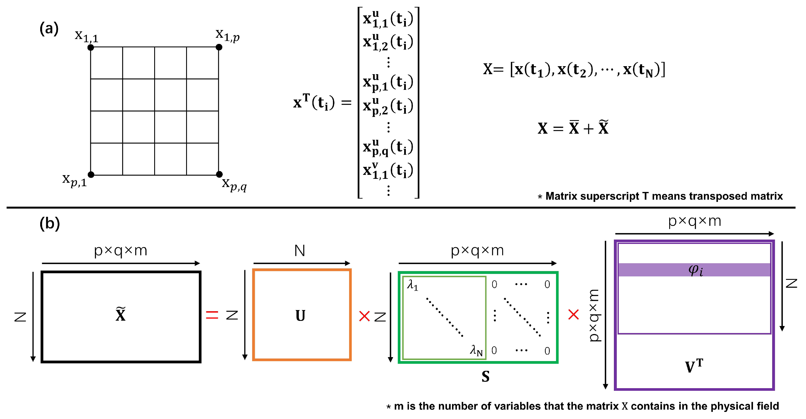
2.3. The Principle of Proper Orthogonal Decomposition

In this work, the Singular Value Decomposition (SVD) POD [24] was applied for a direct decomposition of the selected variable X of a buoyant flame. As shown in the diagram of the SVD method (Figure A3), the input matrix $\overline{X}$ is the instantaneous physical field and can be divided into an average field X and a fluctuation part $X^{\prime }$. The $\overline{X}$ is obtained by time-averaging the input data, while $X^{\prime }$ is obtained by subtracting the $\overline{X}$ from X. Decomposed by the SVD, $X^{\prime }$ can be transformed into the product of three matrices:

$$X^{\prime }=U\times S\times V^T$$

(13)

If $X^{\prime }$ is a $p\times q$ matrix, then the $X^{\prime T}{X}^{\prime }$ matrix is a $q\times q$ symmetric matrix, which can be orthogonally diagonalized, and its eigenvalues ${\sigma }_i$ and eigenvectors $v_i$ can also be obtained. After normalizing the eigenvectors, the orthogonal matrix V is obtained. Then, its singular values are related to the eigenvalues of $X^{\prime T}{X}^{\prime }$, satisfying ${\lambda }_i=\sqrt{{\sigma }_i}$ and greater than zero. The singular values form the S-diagonal matrix as the main diagonal elements. For U, its column vectors can be calculated using $u_i={\displaystyle \frac{1}{2}}{X}^{\prime }{v}_i$ and combined to obtain the U-matrix. Finally, obtaining U, S, and V satisfies the $X^{\prime }=U\times S\times V^T$ relationship. The value of ${\lambda }_i$ on the diagonal is highly correlated with the energy contained in each mode and is considered as the amplification factors [34]. The energy content of each mode is calculated by ${ϵ}_k={\displaystyle \frac{{\lambda }_k}{{\sum }_{i=1}^N{\lambda }_i}}$.

$A=U\times S$ is the time coefficient matrix of the POD, representing the change in each mode over time [35], and the first n column vectors of $\times V$ are the basis vectors obtained by decomposition, which are used to reconstruct the original data field. Usually, the energy associated with the first several modes is much higher. As such, the $X^{\prime }$ can then be reconstructed effectively by using a limited number of modes through

$$X^{\prime }\approx \sum _{i=1}^N{a}_i{\varphi }_i(k<N)$$

(14)

where $A=[a_1,a_2,\cdots ,a_N],V=[{\varphi }_1,{\varphi }_2,\cdots ,{\varphi }_N,\cdots ]$. In addition, those chosen modes often correspond to the critical characteristics of the original physical field.

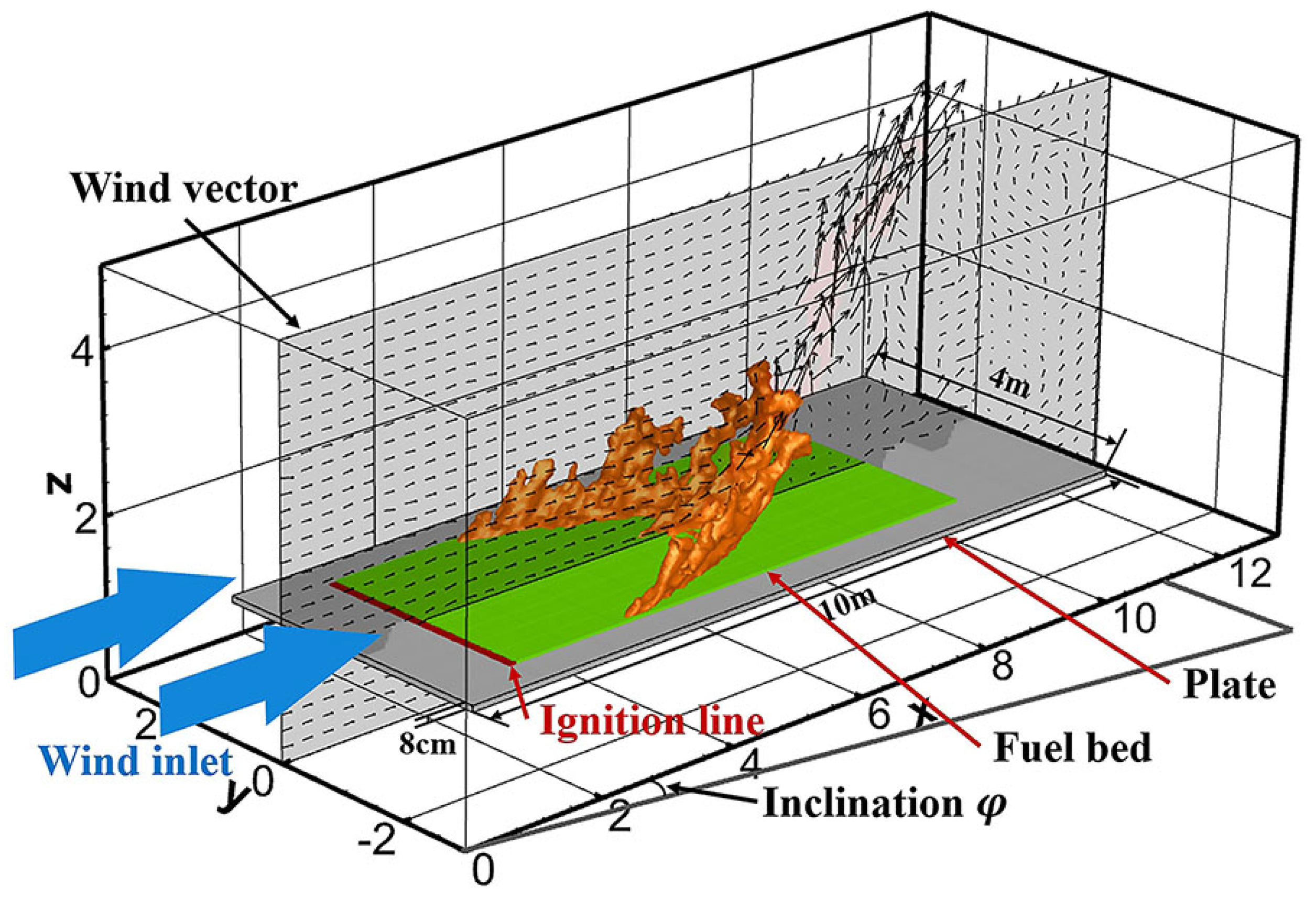
2.4. Experiments and Numerical Setup

Referring to the experiment of Silvani et al. [14] and the DESIRE bench used in the INRA laboratory [13], a large-scale bench 10 m long and 4 m wide was considered for modeling. Therefore, as depicted in Figure 1, the chosen computational domain for this study was a block region (13 m × 6 m × 5 m), and all borders were set as open boundaries except the bottom ground. Within that domain, there was an 8 cm thick plate of 10 m × 4 m to hold the fuel bed. The leading edge of the plate was 1 m away from the open boundary, and the same for its height from the ground.

The wind was introduced from the left side of the domain with the turbulence imposed using the Synthetic Eddy Methodology [21], where the turbulence intensity was set as 20% of the mean velocity. The wind was set parallel to the surface of the fuel bed even when the slope was changed. The fuel bed, measuring 3 m × 7 m, was ignited as a line fire along the left edge by an ignition line of 3 m × 0.1 m, which delivered a power of 500 kW for a duration of 5 s. To ensure a fully developed wind field across the domain, the ignition was delayed with 25 s after the start of the simulation. The calculated profile of the wind speed at the downstream location of 6 m is shown in Figure 2. The radiation fraction was determined from the smoke points ($L_{sp}$) as:

$${\chi }_{rad}=0.41-0.85L_{sp}$$

(15)

where $L_{sp}$ was set based on the measurement in the Fire Propagation Apparatus [36] (i.e., $L_{sp}$ = 0.08 m).

The rate of fire spread is the important parameter to characterize how fast fire propagates into the unburned region, for which the fire front needs to be first properly defined. However, there is still no rigorous definition due to the complex fuel and violent fire, although some prior works attempted to measure it based on the pyrolysis temperature (400 K) [32] or ignition temperature (623 K) [37]. In this work, due to the use of a detailed pyrolysis model, the pyrolysis characteristics of the fuel could be derived (as shown in Figure 3). We can observe that above 560 K, the drying process of virgin fuel was initialized, and shortly afterwards, the intense decomposition reaction was induced, which indicated the usefulness of that temperature as the threshold to differentiate the thermal state of the fuel bed. Thus, that temperature value was adopted in this work to localize the instantaneous fire line.

To determine the appropriate grid resolution, a thorough analysis of the simulation results based on different sizes of mesh and domain was first performed: three sets of domain and grid sizes were examined, respectively, with the smallest mesh size being 0.02 m and the largest domain extending to 14 m in the streamwise direction. It was observed that the computed results were more sensitive to the mesh size compared to the dimension of the domain (shown in Figure 4). Therefore, after a parametric study, a computational domain of 13 × 6 × 5 m and a grid size of 0.05 × 0.05 × 0.04 m were chosen for the later discussion. It has been suggested that to resolve the fire spread on a fuel bed, the grid size needs to be smaller than one-third of the extinction length [23], which was 0.0547 m in the present study. The final mesh used was smaller than that value. Figure 5 depicts the simulated fire front at different instants under a ${30}^{\circ }$ slope and windless conditions. In general, the simulation reproduced the time evolution of the wildfire perimeter observed in the experiments. The comparison with the experimental work of Li et al. [38], depicted in Figure A1, further shows the validity of the present models.

Finally, to conduct a systematic study of the combined slope–wind effects on the fire dynamics, simulation cases with five different slopes (ranging from $0^{\circ }$ to ${30}^{\circ }$) and three wind speeds (0.5, 1.0, and 1.5 m/s) were considered (see

Table 2. Summary of simulation conditions.

	$0^{\circ }$	${10}^{\circ }$	${20}^{\circ }$	${25}^{\circ }$	${30}^{\circ }$
0.5 m/s	✓	✓	✓	✓	✓
1.0 m/s	✓	✓	✓	✓	✓
1.5 m/s	✓	✓	✓	✓	✓

). We also compared the computed fire lines using the newest version of FDS (6.9.1), which showed a close match with present computations (shown in Figure A2). Overall, the present fire modeling was adequate for a thorough analysis of fire dynamics under different wind and slope conditions.

3. Results and Discussion

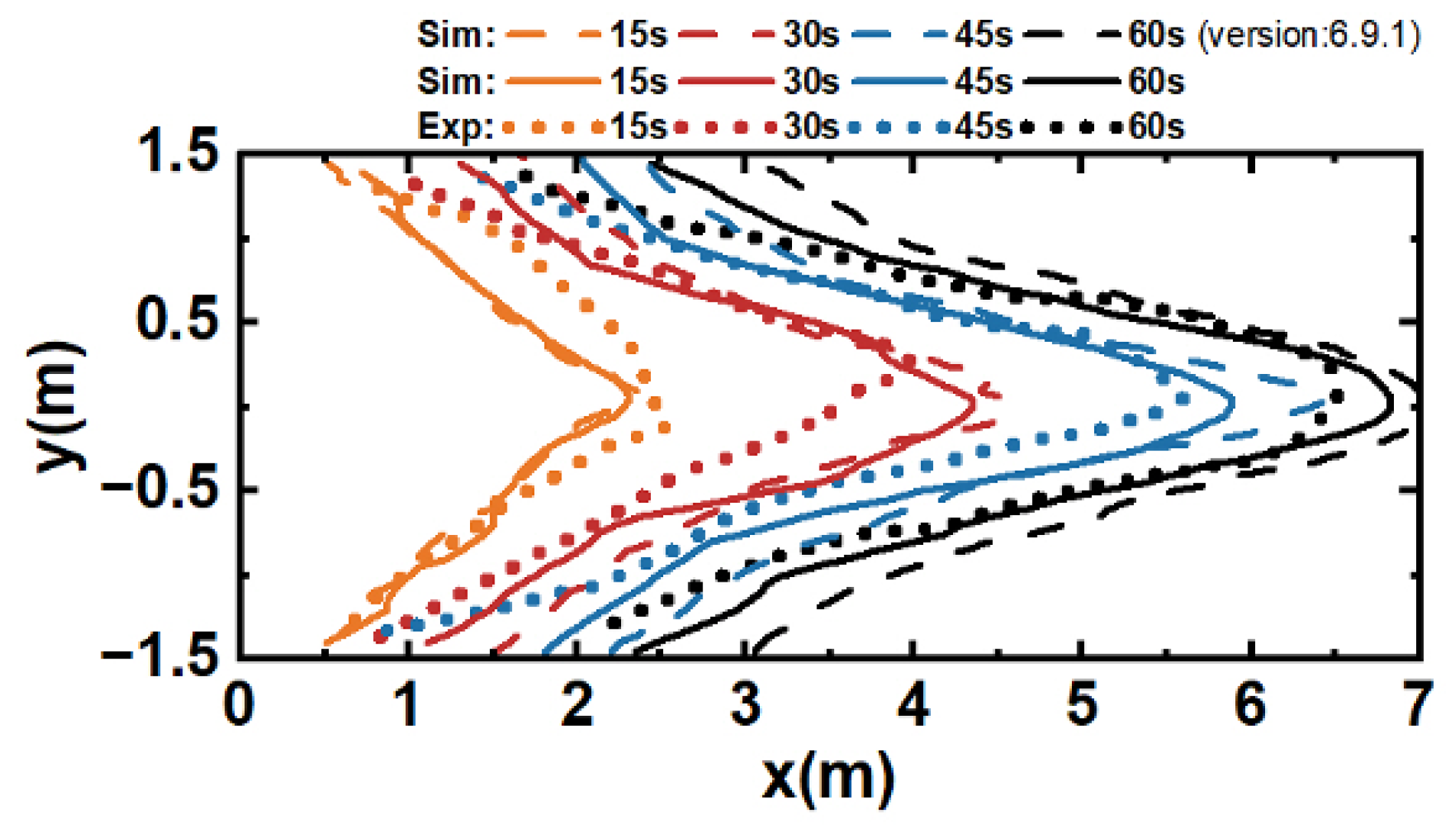
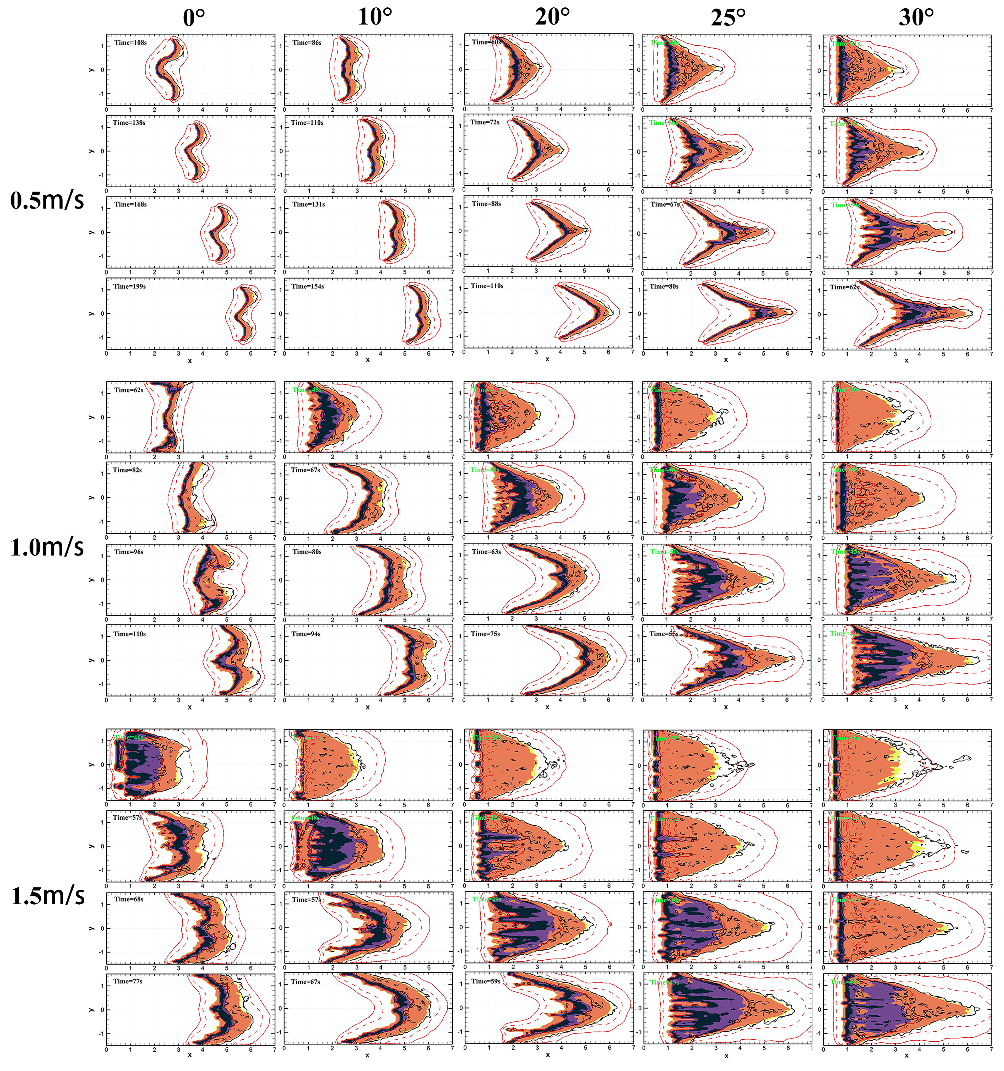
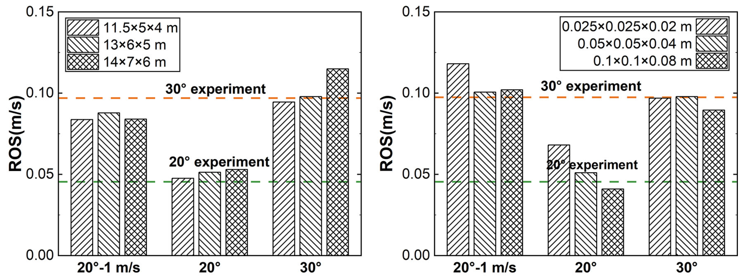
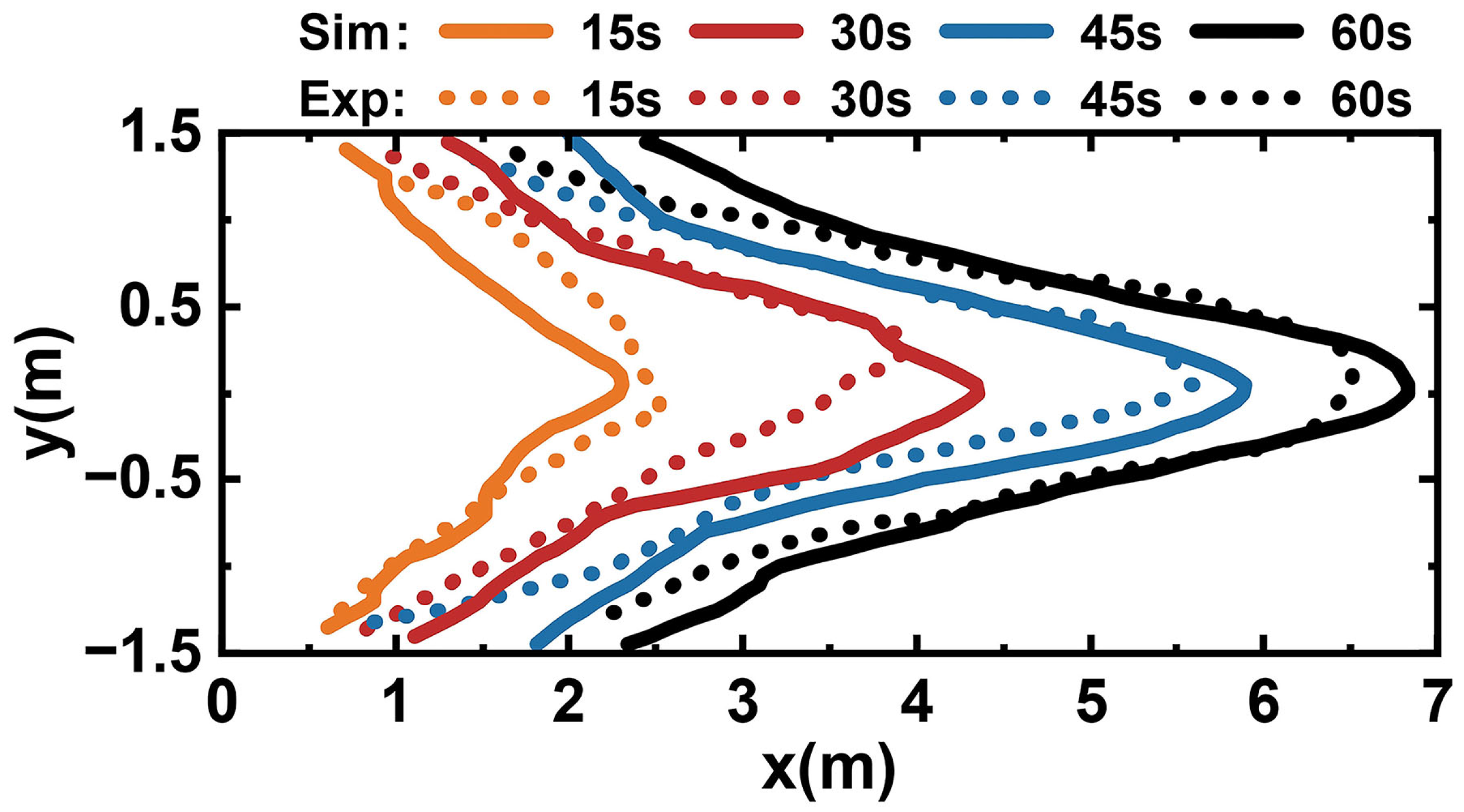
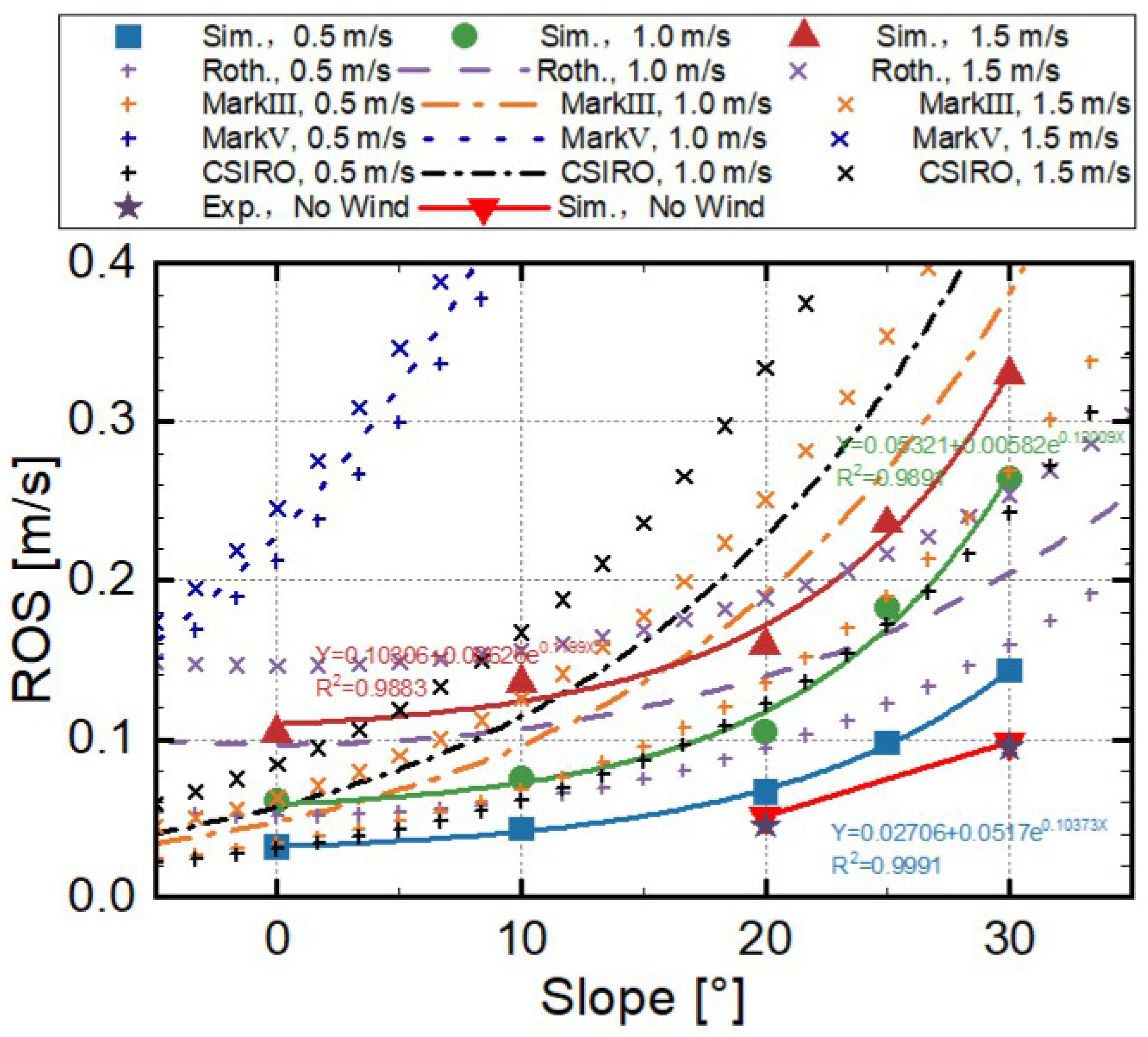
3.1. Fire Perimeter and Rate of Spread (ROS)

Figure 6 first presents the time evolution of the fire perimeter extracted from the representative slope–wind conditions and the topmost cross-section of fuel bed (complete results are provided in the appendix of Figure A4), which are also overlaid with the isolines of convective and radiative heat fluxes received by the fuel bed. A dramatic change in fire topology was clearly seen for different ambient conditions. In most cases, a common pattern of a U-shaped fire line [13] was observed, in particular, for the intermediate values of slope from ${10}^{\circ }$ to ${20}^{\circ }$. With the increase in wind speed (Figure 6b,c), the flame front apparently broadened in space, and at the same time, more stripe burning zones appeared behind the front line. This indicated faster propagation but incomplete combustion under the strong wind conditions. As shown by Porterie et al. [39], a side wind can cause the continuous oxygenation of the fuel bed, promoting the combustion, but at the same time, a strong wind may result in a cooling effect behind the flame front.

A deep change in the fire line shape was found for the slope effect (see Figure 6b,d). Apart from the transformation of the fire shape from a U to a V, the flame front appeared to be no longer compact but more distributed within the central region, indicating an acceleration of the fire spread along the axis on the sloped terrain. As discussed in earlier works [13,14], this fire behavior could be ascribed to the tilted and elongated flame volume as well as a coupled effect from the fire-induced turbulent motion. The latter one may enhance the heat transport through convection. As shown in the plots, the convective isolines fluctuated more under that condition. Furthermore, its distribution was close to the fire line, confirming the dominated role of turbulent heat convection in the vicinity of the fire line. This is an important supplement to existing studies since it is difficult to be measured in experiments. The radiation has often been assumed to govern the fire spread, but in most cases, the temperature rise of fuel particles and their subsequent ignition are convection-controlled because the heat transfer coefficients for free and forced convection depend on the inverse function of the characteristic surface length [40].

The larger spatial distribution of the radiative heat flux (red isoline) in comparison to the convection part (black isoline) beyond the fire front also implied that in this study, the radiation may have dominated the preheating of the combustible bed. At the same time, it is interesting to note that the enlargement of the dominated area of the radiation heat flux was more sensitive to the increase in wind speed than that of the slope.

This study also discovered another intriguing phenomenon: under a low wind speed and in sloped environments, the fire front deformed into a W-shaped structure with two flame heads (Figure 6a). This is elaborated on in detail later.

Subsequently, to quantitatively evaluate the influence of the slope and wind on the fire spread, the rate of spread (ROS) was calculated by post-processing the time-averaged fire lines under different ambient slope–wind conditions. Figure 7 illustrates the ROS computed for various slope and wind cases. Additionally, results calculated using the empirical models [21], such as the Rothermel model, CSIRO, MarkIII, and MarkV [23] are also presented. The experimental data were only available for the windless conditions. In general, the ROS increased with the increase in slope, and this trend was almost the same for the three considered wind velocities. Specifically, the change in ROS was a linear function at a lower slope and when the slope was higher than ${10}^{\circ }$, a nonlinear increase was observed for all side winds, which indicated the existence of a universal critical slope regardless of wind speed to enhance the conjunct effects of slope and wind and hence induce an eruptive fire [16].

The predictions from the empirical models generally departed from the present physics-based simulations. However, in comparison, except for the apparent deviation after ${10}^{\circ }$, MarkIII showed a closer match in small-slope conditions ($0^{\circ },{10}^{\circ }$). This could be attributed to the simplified assumption and the specific experimental scenarios used for deriving these empirical formulas.

Figure 8 shows the variation in ROS when increasing the wind speed conditioned on different slopes. Compared to the observation shown in Figure 7, the fire line spread more linearly with the increased wind. However, the acceleration of the spreading fire seemed to be less sensitive to the wind increment at the higher slope (e.g., ${30}^{\circ }$), which indicated the prevailing influence of the slope even when the wind speed was high. It also implied that the mechanism controlling the fire spread with the increase in slope and wind, respectively, was different, which is further explored in the later discussion.

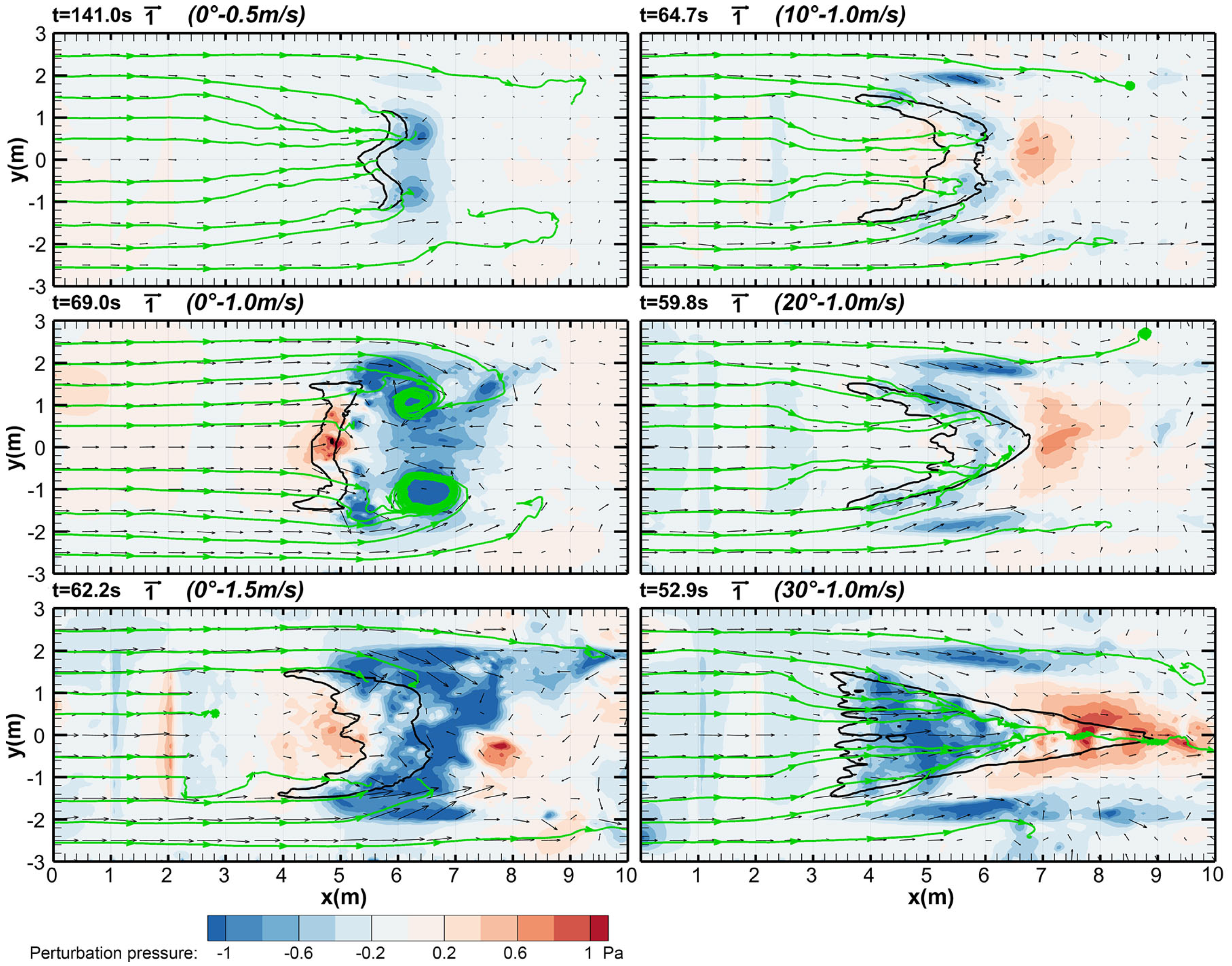
3.2. Flow Field and Perturbation Pressure

To better understand the individual wind and slope effects on the fire spread process, Figure 9 illustrates the velocity field and perturbation pressure contour in an x–y cross-section computed under three wind speeds without any slope and three different slopes with a 1 m/s wind speed, respectively. It can be observed that without a slope, under the effect of ambient wind only, the fire line tended to exhibit a concave shape at the center region, forming a W-shaped structure with two heading flames. This can be attributed to the pair of vortices and a negative pressure zone formed in front of the leading edge. With the increase in wind speed, however, the apparent big eddy dissipated because of the strengthened wind speed, and at the same time, the more pronounced enlargement of the negative pressure zone showed that the wind effect could be understood from the induced turbulent flow field, which developed a strong fluctuating buoyant plume with the fresh air largely entrained from the front side of the flame. The low-pressure zone was also observed experimentally by Clements and Seto [6]. They pointed out that the pressure minimum may be responsible for the observed acceleration of horizontal flows into the fire and the strong updraft, as shown in Figure 10.

In contrast, for the sloped terrain, even with ambient wind present, the region ahead of the fire front tended to be under the influence of a positive pressure instead of a negative one. Moreover, the strength of the positive pressure increased with steeper terrain. Therefore, it can be inferred that the concavity of the fire line at $0^{\circ }$ was mainly caused by the entrainment of the lateral airflow and the backflow induced by the turbulent fire plume; the corresponding pressure drop suppressed the central fire spread and alternatively promoted the movement of the lateral heading fire. However, with an increase in slope angle, due to the inclination of the flame, the flame region expanded closer to the unburned area ahead, resulting in the higher possibility of high-temperature gas flowing over the unburned vegetation. This led to the suppression of the backflow and the formation of a high-pressure zone. A faster spread of the central fire heads was then expected, forcing the fire line to develop into a pointed V shape. As indicated by Hassan et al. [41], for the V-shaped fire line, the interaction between the two junction arms is another critical factor, enhancing the fire dynamics.

The flow field in the x–z cross-section shown in Figure 10 clearly illustrates the complex change in flow pattern above the unburned fuel bed under the different ambient conditions. The dominating influence of the wind (left-side plots) creates a complex turbulent flow, interacting with the flame-zone buoyancy. The slope effect, on the other hand, can be seen as the suppression of the indraft flow ahead of the flame due to the strong buoyant flow, and thus the promotion of the hot-temperature gases convected from the fire-front region to the inert vegetation fuel. In the field of establishing the operational model for fire spread prediction, the slope effect is usually modeled by assuming that it acts like the ambient wind [42]. However, the present analysis implies that although both wind and slope could lead to the flame inclination, the fluid dynamics induced near the fire front would be totally different; in particular, the difference in flow of the frontal area could impact the influential region of convective heating or cooling. Properly modeling this difference may be the key to capturing the erratic fire spread at higher slopes.

In addition, it is interesting to note the convergence of the incoming wind field from the profiles of the streamline in the x–y cross-section (especially the case of ${30}^{\circ }$–1.0 m/s in Figure 9). It was associated with the stream-wise streaks of flame behind the flame front as reported by Finney et al. [40]. A saw-toothed flame geometry was then observed, which was related to the complex flow dynamics of Taylor–Görtler instability and the vegetation smoldering combustion due to the fast fire spread.

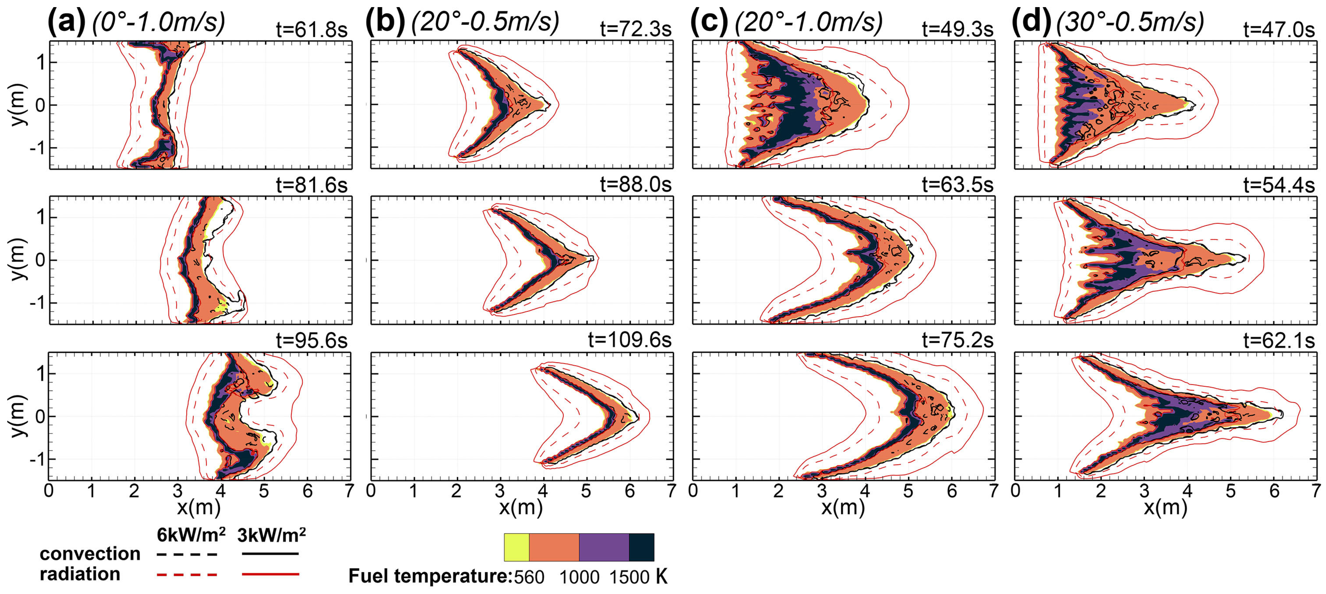
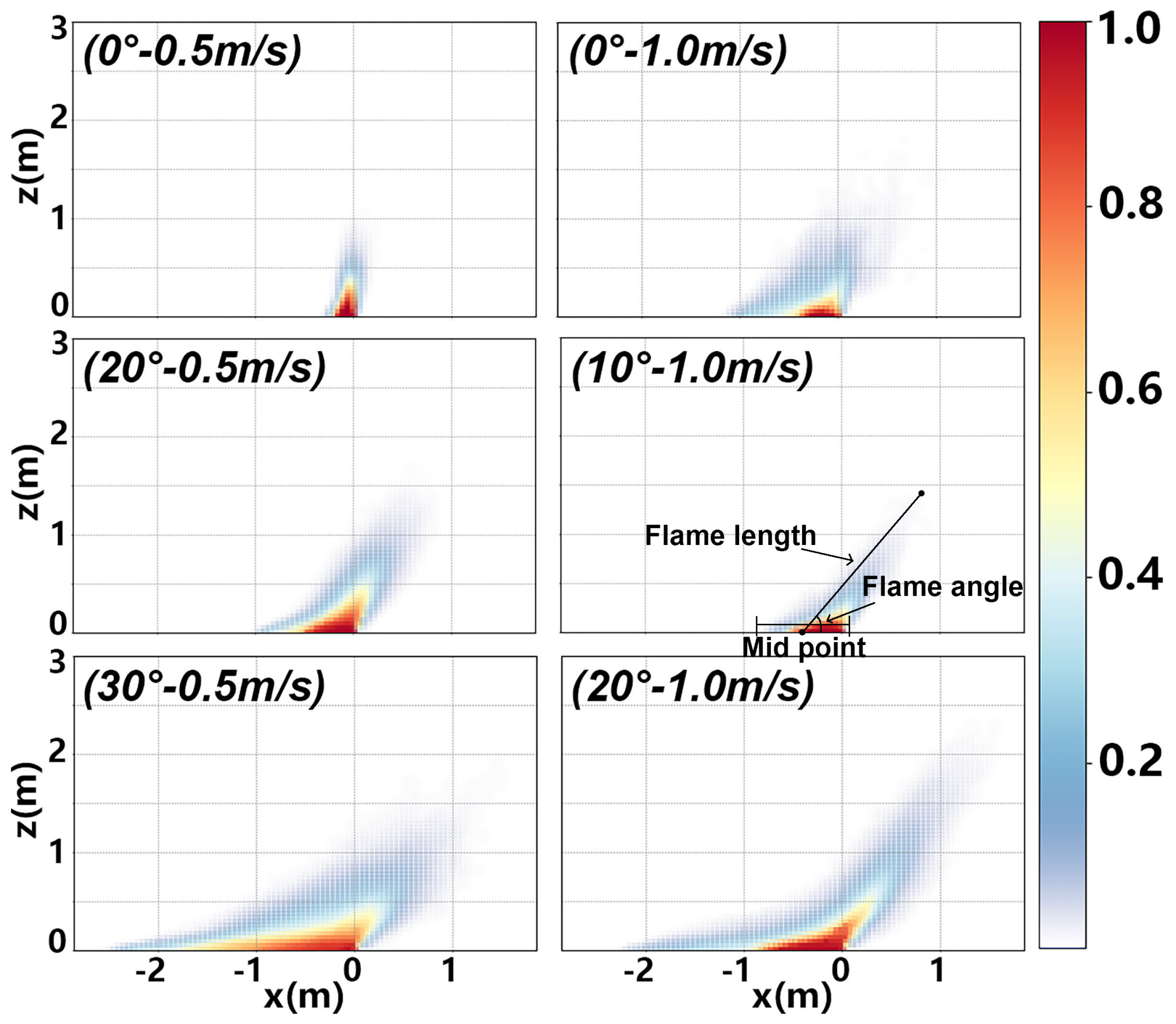
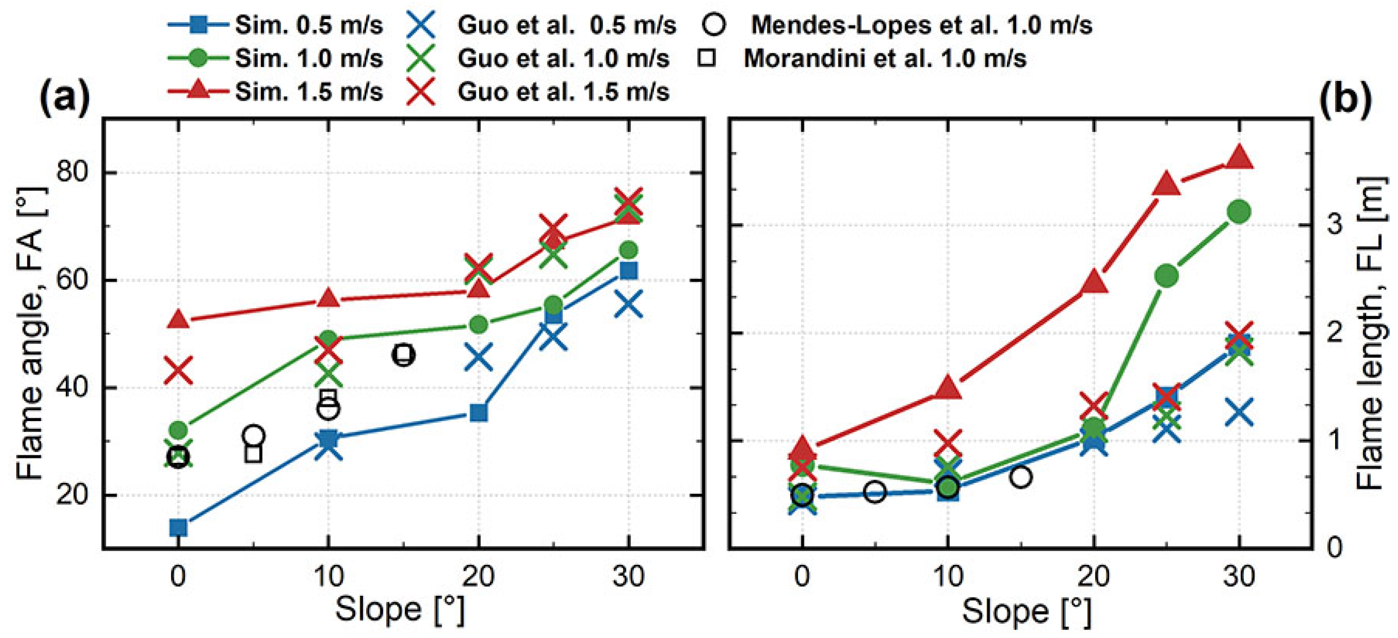
3.3. Flame Morphology

To understand the abrupt change in the speed of the spreading fire shown in Figure 7, it is useful to analyze the flame topology, which is key to determine the heat transfers to the vegetative fuel [14,16]. As revealed above, the ambient condition showed the determining effect on the fire propagation through the marked change in flame dynamics. Therefore, the specific parameters pertaining to the flame morphology and to the easy understanding of the slope–wind effect are discussed. First, there are various methods to define the flame region, and in experiments, the averaged luminous region captured by the camera is most often adopted to extract the flame shape [11].

However, in simulations, numerous parameters can serve as the indicator of the flame zone, including the temperature, heat release rate, combustible gases, and oxygen concentration [43]. Given that the combustion model was an Eddy Dissipation Concept (EDC) combustion model based on a mixed fraction, where the chemical reactions were primarily depending on the mixedness of the vapor fuel and oxygen, we therefore chose the fuel gases as the variable to define the flame region. Based on the analysis of the flame profiles, it was found that the exothermic reaction zone was primarily located within the region where the fuel mass fraction $Y_f$ was less than 0.001. Therefore, this critical value was adopted as the threshold to define the flame shape.

By employing $Y_f$ = 0.001 as the threshold to create the binary image and extract the instantaneous flame front, and adopting the right corner of the flame base in the x–z plane as the reference point, the contours of the time-averaged flame probability for different conditions were obtained, as shown in Figure 11. It is seen that in general, apart from the case of $0^{\circ }$–0.5 m/s, the flames in other conditions tilted further towards the unburned area and at the same time, the flame was significantly elongated.

The flame angle (FA) and length (FL) (illustrated in Figure 11) are two critical geometry parameters that can help illustrate the heat transfer processes, the driving force for the fire spread. Following earlier works [13,44], they were calculated in this study based on the same process as that to define the flame probability contours. Figure 12 shows the profiles of the computed flame angle and length in a comparison to the experimental results of Guo et al. [44], Morandini et al. [45], and Mendes-Lopeser et al. [46] It can be observed that the increase in slope and wind speed led to an increase in both flame length and angle, and in particular, after an almost linear change between $0^{\circ }$ and ${20}^{\circ }$, a sharp increase was found after ${20}^{\circ }$, indicating the existence of a critical slope angle for the transition from the normal fire spread to the abrupt acceleration [16].

Comparatively, the present simulations reproduce the general trend reported in earlier measurements. This is particularly notable given that errors may arise from the differences in fuel bed parameters (e.g., fuel depth and bench size) and the method used to determine the flame shape. However, due to a closer match between the simulation and the experiments for FA, the result implies that the flame angle might have a smaller sensitivity to the fuel bed properties as also indicated in the work of Sánchez-Monroy et al. [22].

Overall, together with the variations observed in the flame probability contours, the remarkable changes in flame length and angle indicate that the higher wind and slope allows the flame to approach further the unburned fuel bed, increasing significantly the contact area for radiative heat transfer. This is manifested visually in Figure 6 for a larger impact area of radiative heating under the high slope and wind conditions. Meanwhile, the expanding flame volume and the plume-induced circulation flow would induce a substantial amount of high-temperature gas to flow over the unburned fuel ahead of the fire line. This significantly enhances the convective heating. Thus, the enhancement of both convective and radiative heat transfer modes is often regarded as the driving force for the nonlinear behavior of the fire spread under different ambient conditions [14,16,22]. In addition, at a higher slope (30°), the flame inclines almost parallel (FA > 60°) with respect to the fuel bed, which promotes the probability of flame attachment on the unburned fuel surface.

It was noted that the flame attachment could be the main reason for the development of the extreme or erratic fire spread [16]. To have a better illustration, the flame attachment length was defined here by measuring the distance between the flame front position on the surface of combustible fuel particles and the pyrolysis front position, as shown in Figure 13 under different ambient conditions. On the horizontal axis, $t_{\mathrm{ign}}$ denotes the duration of the initial ignition stage. It can be seen that as expected, this attachment length increased with the increase in wind speed; however, a more pronounced change was observed for the slope effect especially when the slope angle increased from ${20}^{\circ }$ to ${30}^{\circ }$, which may explain the abrupt rise in ROS by a factor 2–2.5 observed both in Figure 7 and in the laboratory studies of Dupuy and Maréchal [13].

In addition, it is also worth noting that the FA and FL both seemed to show high dependence on the slope of the terrain while the FL was only more sensitive to the wind speed. This is consistent with the observations in Figure 9 and Figure 10; the wind effect caused a backflow ahead of the flame front, which, however, was restrained by the high-pressure zone in sloped conditions, and the slant flame or the tilted angle was therefore more pronounced for the slope effect.

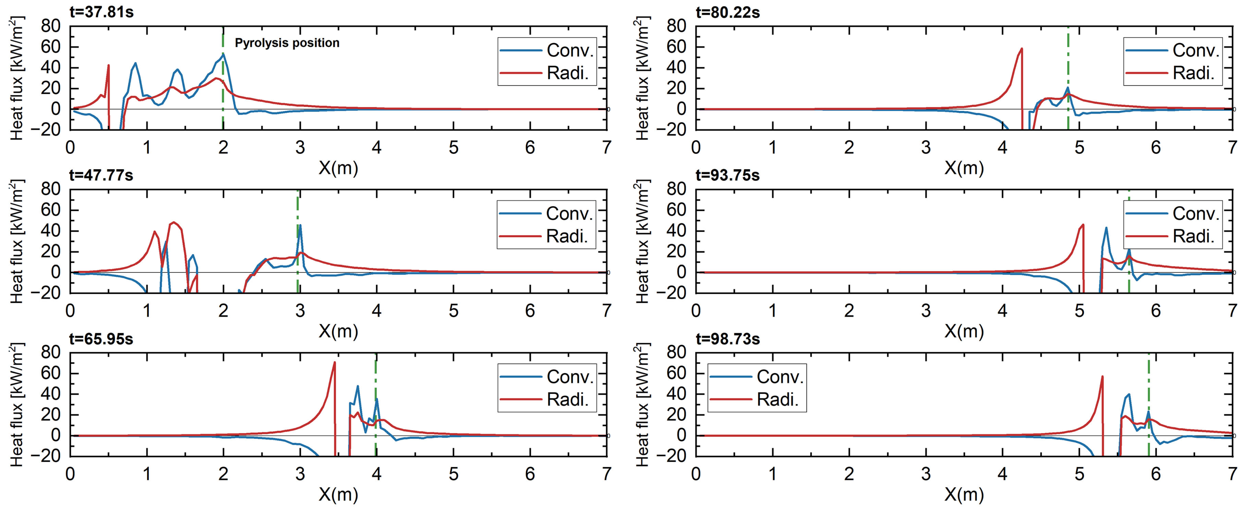
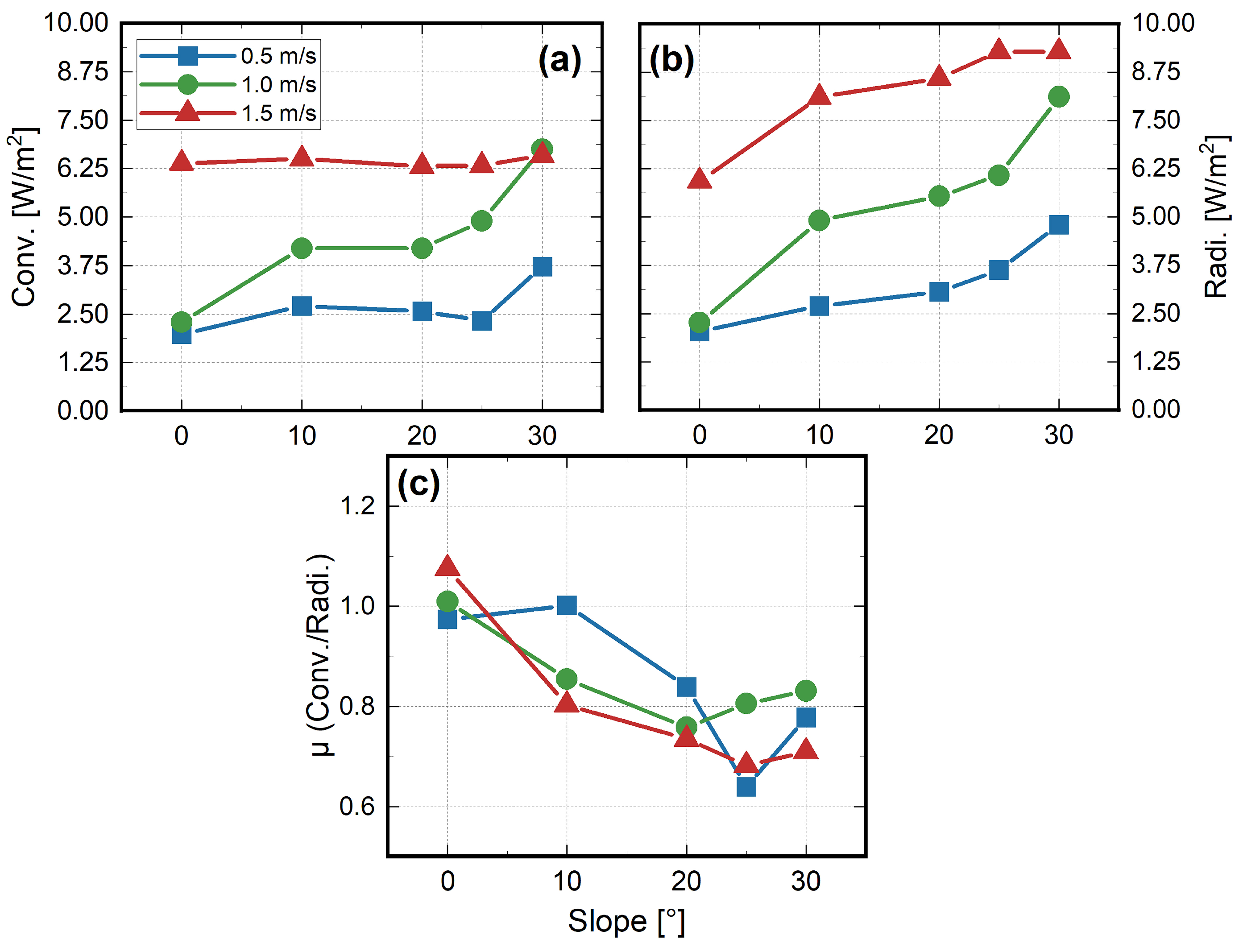
3.4. Radiative and Convective Heat Transfers

A quantitative evaluation of the thermal budget (i.e., convective and radiative heats) was conducted to further understand how the heat transport was controlled by the slope and wind effects and its feedback on the fire-line dynamics. Figure 14 first presents the instantaneous profiles of the convective and radiative heat fluxes absorbed by the unburned fuel near the fire front along the centerline. It is seen that in the initial stage of ignition, the absorbed heat budgets were large, after which the magnitude of received energies became smaller and their distributed area tended to be stable. Close to the fire front (denoted by the vertical dash-dot line), the influential domains of positive convection and radiant heating were almost overlaid with each other except the area far behind and ahead of the fire, where heat transport was dominated by radiation. The fire-induced turbulent convection enhanced the intermittent presence of hot gases impinging on top of the inert fuel, which even overwhelmed the heat budget close to the fire front. This indicates the invalidation of the simplified assumption, i.e., the neglected convective heating, adopted in many empirical fire spread model [45]. In addition, the negative regime of both convection and radiation heating behind the fire line corresponded to the locations of exothermic char oxidation with a high temperature, and the incoming wind flow mainly introduced a cooling effect.

To focus on the heating fluxes that were responsible for fire spreading, the time average over a domain, ranging from the fire line to the isoline of zero convective heat flux ahead, was employed to obtain the averaged heat components (convection and radiation). Figure 15 presents the averaged heating fluxes of convection and radiation under different conditions. The radiative heating showed a more dramatic increase with the rise in wind speed and slope. For the case of a 1.5 m/s wind velocity, however, its increase became milder with the change in slope, indicating the less dominated effect of the slope at high-wind-speed conditions. On the other hand, the convective component showed a considerable change only after the critical slope angle of 20°, which resembled more the trend indicated by the flame angle in Figure 12.

This may be explained by the fact that different mechanisms could exist for the radiative and convective heat transports, respectively: the radiation heat flux is controlled by the combined effects of the flame length and view angle that determine together the amount of heat transport between the radiant surface of the flame and the fuel bed. Conversely, the convective part of the heating flux is dominated by the action of the flame attachment, and therefore, it is only more dependent on the tilted angle.

Therefore, the heat transport through the convection and radiation showed a different pathway during the change in wind speed and slope, within which the flame morphology played a critical role. The ratio of their magnitude shown in Figure 15c further illustrates that the strength of the convection was still smaller, but the enhancement of the convection part of heating would be the main factor for accelerating the fire spread under steeper slopes (especially above 25°) [16]; in the case of a 30° slope, the convective heating accounted for almost half of the heat gain. In addition, the decreased role of the radiation part when the slope angle rose above 20° was consistent with the observation in experiments of Dupuy and Maréchal [13].

To further elucidate the mechanism governing the heat transport for fire propagation, the Byram convective number ($N_c$) [47], denoting the ratio between flame buoyancy and inertial force, was calculated as follows:

$$N_c={\displaystyle \frac{2g{I}_B}{\rho C_{p}T(u-ROS)}}$$

(16)

where g is the gravity, and $\rho$, $C_p$, and T denote the density, specific heat capacity, and temperature of ambient air, respectively. u is the wind speed, and $I_B$ is the fire line intensity. For the scenarios considered in this work, the calculated $N_c$ values are presented in

Table 3. Byram convective number $N_c$ calculated for different slope and wind conditions.

	0.5 m/s	1.0 m/s	1.5 m/s
$0^{\circ }$	122.6	24.4	9.8
${10}^{\circ }$	164.9	27.3	12.6
${20}^{\circ }$	194.4	32.9	15.9
${25}^{\circ }$	247.9	83.3	18.2
${30}^{\circ }$	526.1	103.0	27.8

. For $N_c$ < 2, the fire is wind-driven, and $N_c$ > 10 denotes a buoyancy-dominated fire. A mixed regime for fire propagation is deemed to occur for 2 < $N_c$ < 10.

It is seen from Table 3 that the effects of wind and slope differed from each other: with the increase in wind speed, the propagation mode tended to be wind-driven because of the decrease in $N_c$, and conversely, the fire was more strongly buoyant with the increase in $N_c$ when the slope was larger. In the meantime, the transition of the fire mode appeared to be more sensitive to the change in wind in low-slope conditions (<${20}^{\circ }$), in which a more dramatic change in $N_c$ was observed. In general, for most cases, the fire considered in this work was plume-dominated with $N_c$ greater than 10. The exception was for cases with a wind speed of 1.5 m/s, where $N_c$ was relatively small and the flame propagation was more likely driven by the wind. This may explain the mild change in thermal budget for the 1.5 m/s wind speed shown in Figure 15a,b in different slope conditions. In addition, the abrupt change in $N_c$ at a slope of ${30}^{\circ }$ indicated a stronger fire plume that would increase the flame attachment and accelerate the flame spread.

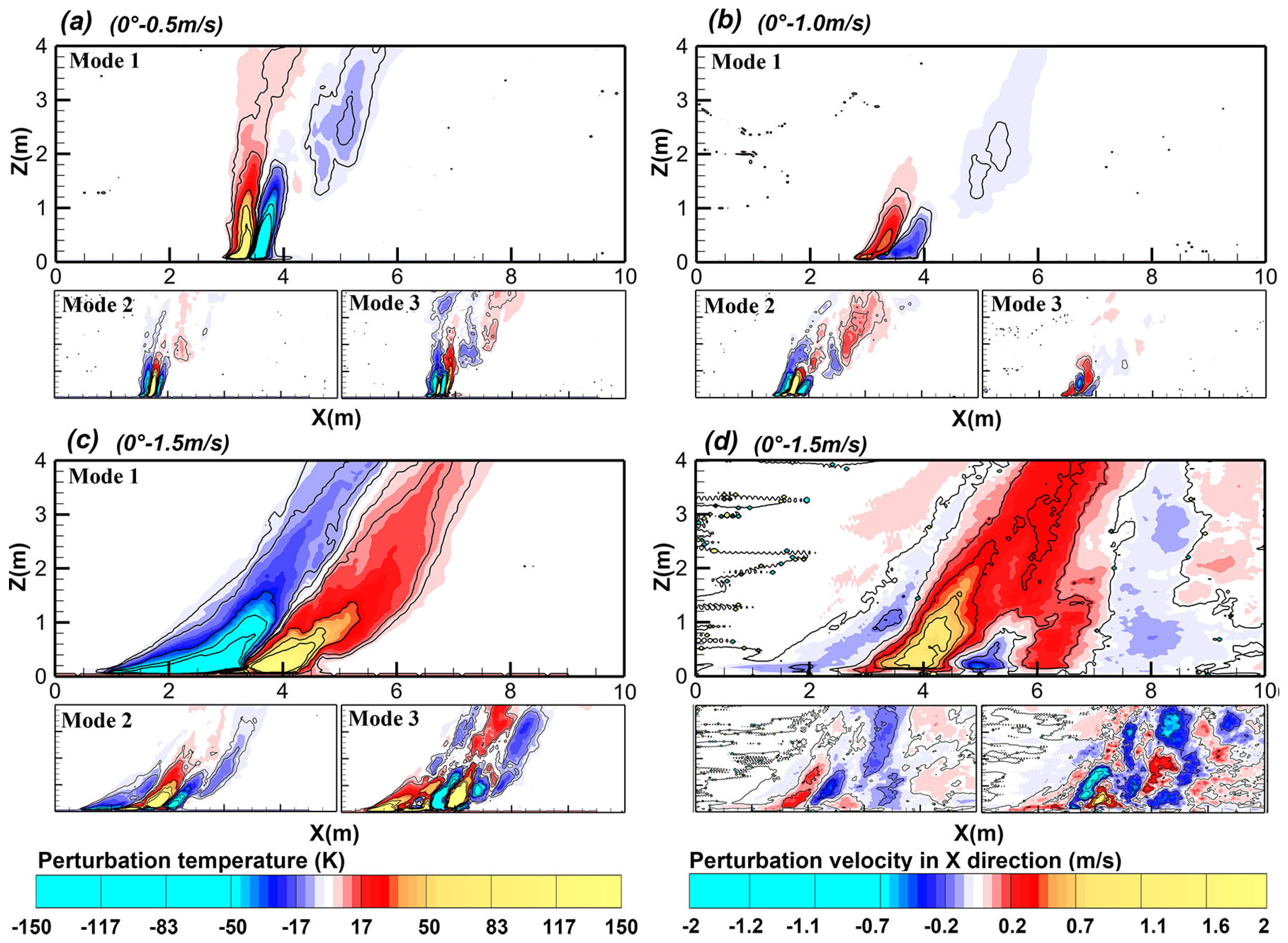
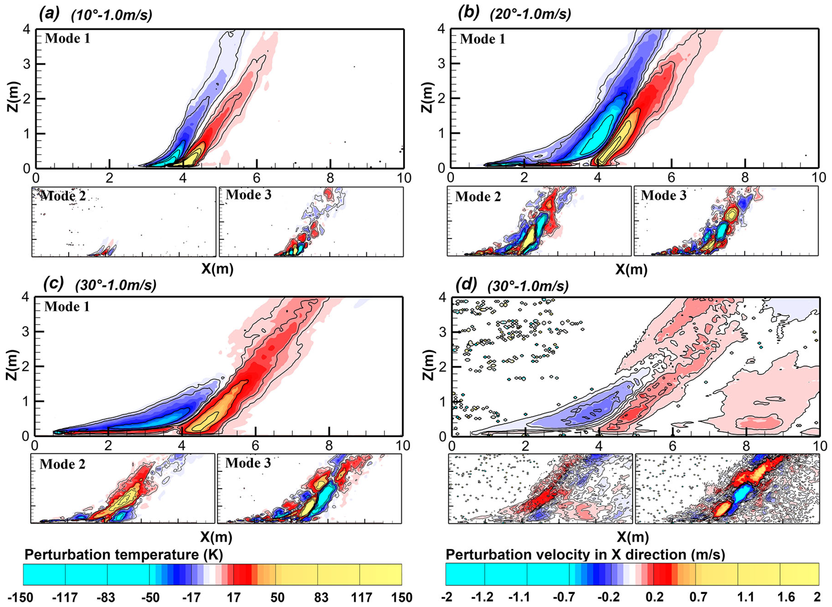
3.5. Proper Orthogonal Decomposition (POD) Analysis

In the intrinsic orthogonal decomposition, new basis vectors (that is, modes) are used to reconstruct the original data, and the degree of representation of different basis vectors on the original data can be represented by the eigenvalue matrix, which is the energy content mentioned earlier. In this paper, a POD analysis was carried out; as shown by the energy content of each mode (k) in Figure 16b, the energy associated with the first several modes was usually much higher.

Figure 16a illustrates the reconstructed temperature field from mode 1 with a propagating fire front in slope–wind conditions of ${20}^{\circ }$–0.5 m/s. It reveals the dominant pulsating features of gas temperature (in red and blue) at the flame base, interacting with the coherent vortex structures (in yellow).

To understand the coherent flame structures under different environmental conditions and their interaction with the turbulent flow fields, the temperature–velocity fields at the wind speed of 1 m/s and angles of ${10}^{\circ }$, ${20}^{\circ }$, and ${30}^{\circ }$ and three wind speeds without a slope were selected as the input data for the POD analysis. The energy distributions of the first 15 modes and their cumulative energy obtained for three different conditions are shown in Figure 16b. Mode 1 occupies an absolutely dominant position, with the second and third modes contributing to a partial share of total energy (approaching 10%). Therefore, in this study, the POD analysis mainly relied on these first three modes.

The reconstructed temperature and velocity fields are depicted in Figure 17 for various wind speed conditions. Dominant mode 1 clearly revealed the primary structural feature of the fluctuating flame front that was in a back and forth mode (in blue and red colors, respectively). The lower energetic modes 2 and 3 showed a similar structure but with three distinct regions and a smaller spatial distribution. This was caused by the fluctuation in the flame and the movement of the flame front. In general, the spatial distribution of different modes increased, and the slant of the flame became apparent when the side-wind became stronger. In the 1.5 m/s case, it is interesting to note that the positive part of the pulsating temperature was located in the front. This means that the influx of fresh air and their cooling effect caused by the backflow ahead of the flame front was suppressed in higher-wind conditions, which is also indicated in Figure 10.

For different sloped terrains, it is shown in Figure 18 that the positive and negative coherent structures under different slope angles were similar to the stronger wind conditions in Figure 17, and in the meantime, for the same wind speed, the mode pattern of the ${10}^{\circ }$, 1.0 m/s wind–speed conditions was distinct from its counterpart with a flat terrain in Figure 17. This indicates that under the slope effect, the intense burning of the fuel bed existed near the fire front and thus, the buoyancy flow and the incoming wind enhanced the temperature rise in the direction of fire plume. As the slope increased, the flame zones tilted further with an enhanced forward pulsation.

For modes 2 and 3, however, the dominant structure was not observed, and it seemed that for those modes, the corresponding flame dynamics were controlled mainly by the small scale of the vortex that generated the fluctuation in the direction of the buoyancy flow, which was different from that observed in Figure 17. It could be found by alternating positive and negative fluctuations. This further demonstrated that the mechanism of the slope effect controlling the fire spread was different from that of the wind speed. For the steeper-slope condition, those structures of turbulent fluctuations tended to enlarge in space, indicating a higher turbulent intensity, which would then strengthen the effects of turbulent convection and heating in front of fire zones. This explains why there exists a critical slope for the acceleration behavior of a propagating fire.

With a 30° slope and 1 m/s wind speed (Figure 18d), the velocity field exhibited a similar phenomenon with fluctuating structures resembling those of the temperature field. The same phenomenon could be seen at different wind speeds.

4. Conclusions

This paper presented a detailed numerical simulation of wildfire, investigating comprehensively the main characteristics of the fires spreading under the combined effects of wind and slope. More specifically, the rate of spread, flame morphology, convective and radiative heat transfers, as well as the fluid dynamics were studied quantitatively in detail, focusing on the fire spreading mechanisms controlled by slopes and wind speeds, for which the physics-based modeling of interactions between vegetal fuel and flame and a POD analysis were employed. The main conclusions are as follows:

• A power-law relationship was found between the ROS and slope angle. It was revealed that in high-slope conditions, the convergence of incoming wind and the weakened indraft air from the frontal area made a significant contribution to the abrupt rise in ROS and the eruptive spread of the head fire. As the slope increased, the flame also approached the combustible material under the action of gravity. As the slope gradually increased, the flame eventually coincided with the combustible material ahead, leading to a rapid increase in convective heat transfer.
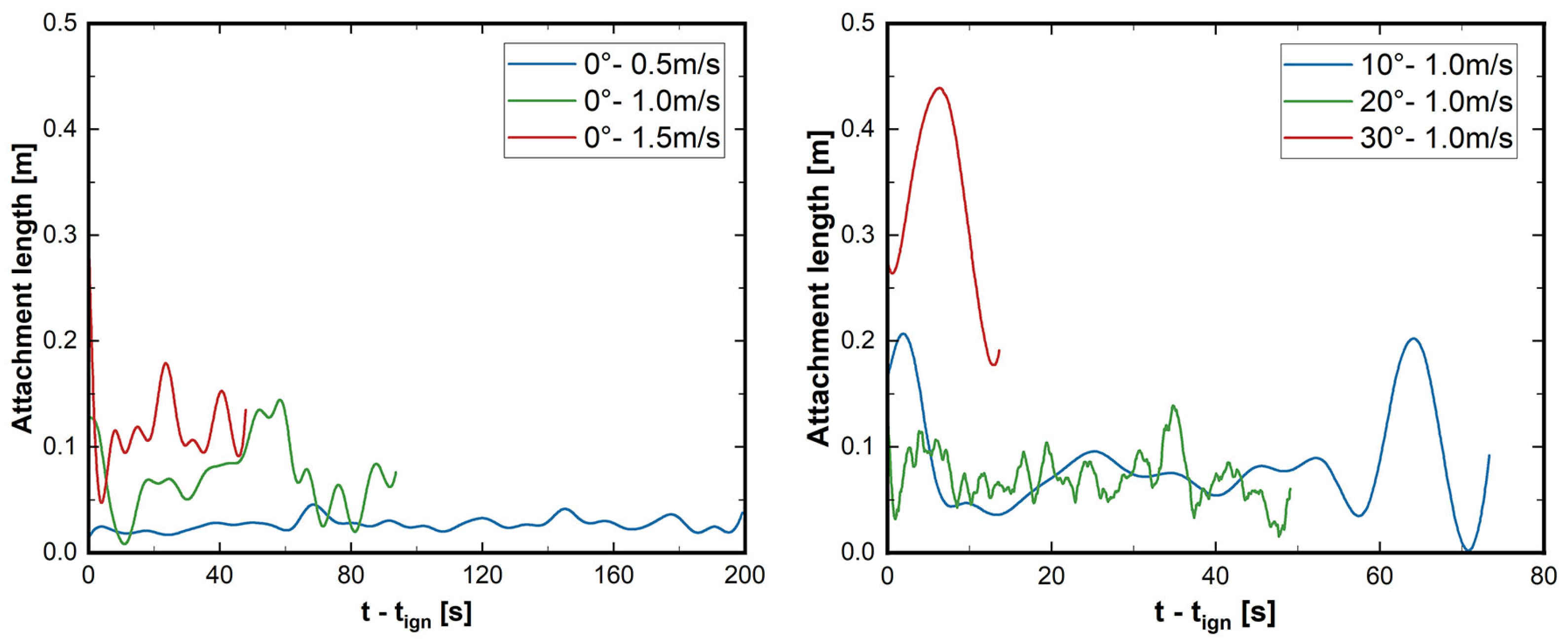
• The enlarged volume of the fire plume was deemed to enhance the radiation heat transfer, and in contrast, the higher possibility of flame attachment at higher slopes (especially >20°) led to the prominent role of convective heating. When a flame attached to a wall, convective heat transfer significantly increased compared to radiative heat transfer.
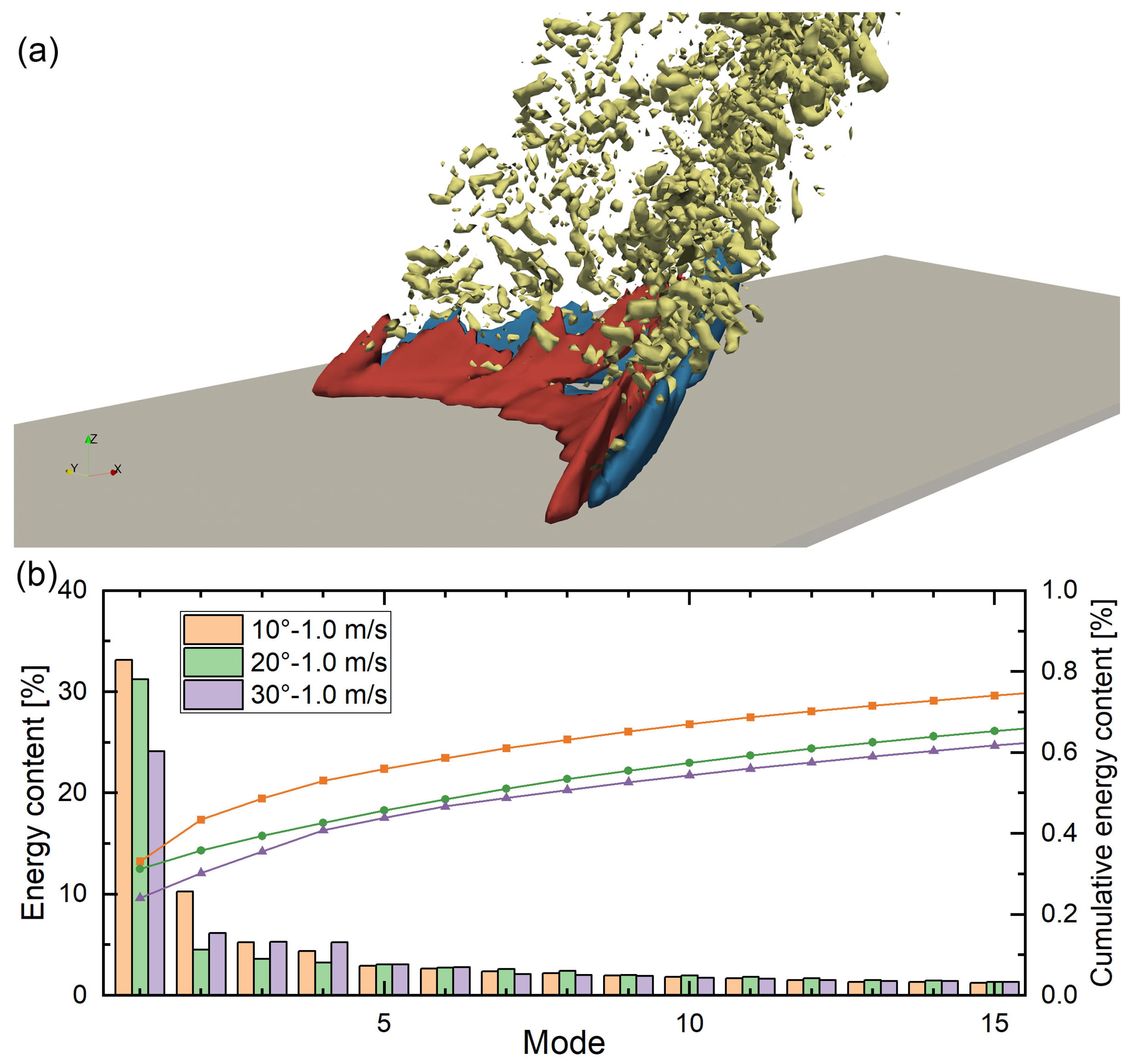
• The investigation into the joint temperature–velocity field utilizing a POD approach revealed an increased forward pulsation of the flame front with the escalating slope, leading to a higher energy density in the pre-combustion zone ahead of the fire line, which further explained the mechanism underlying the accelerated flame propagation.
• For wildfire modeling, the more decent model should distinguish the respective roles of wind and slope, where the slope has a more profound effect in terms of determining flame structures and convective heat; the unsteady feature of flame puffing could be incorporated, considering the dominated mode pattern of backward–forward pulsation.

References

1. Gajendiran, K.; Kandasamy, S.; Narayanan, M. Influences of wildfire on the forest ecosystem and climate change: A comprehensive study. Environ. Res. 2024, 240, 117537. [Google Scholar] [CrossRef] [PubMed]
2. Folharini, S.; Vieira, A.; Bento-Gonçalves, A.; Silva, S.; Marques, T.; Novais, J. Bibliometric Analysis on Wildfires and Protected Areas. Sustainability 2023, 15, 8536. [Google Scholar] [CrossRef]
3. Kramer, H.A.; Mockrin, M.H.; Alexandre, P.M.; Radeloff, V.C. High wildfire damage in interface communities in California. Int. J. Wildland Fire 2019, 28, 641–650. [Google Scholar] [CrossRef]
4. Or, D.; Furtak-Cole, E.; Berli, M.; Shillito, R.; Ebrahimian, H.; Vahdat-Aboueshagh, H.; McKenna, S. Review of wildfire modeling considering effects on land surfaces. Earth-Sci. Rev. 2023, 245, 104569. [Google Scholar] [CrossRef]
5. Sharples, J.J. Review of formal methodologies for wind–slope correction of wildfire rate of spread. Int. J. Wildland Fire 2008, 17, 179–193. [Google Scholar] [CrossRef]
6. Clements, C.; Seto, D. Observations of Fire-Atmosphere Interactions and Near-Surface Heat Transport on a Slope. Bound.-Lay. Meteorol. 2015, 154, 409–426. [Google Scholar] [CrossRef]
7. Seto, D.; Clements, C.; Heilman, W. Turbulence spectra measured during fire front passage. Agric. For. Meteorol. 2013, 169, 195–210. [Google Scholar] [CrossRef]
8. Kochanski, A.; Jenkins, M.A.; Sun, R.; Krueger, S.; Abedi, S.; Charney, J. The importance of low-level environmental vertical wind shear to wildfire propagation: Proof of concept. J. Geophys. Res. Atmos. 2013, 118, 8238–8252. [Google Scholar] [CrossRef]
9. Sun, R.; Krueger, S.; Jenkins, M.; Zulauf, M.; Charney, J. The importance of fire-atmosphere coupling and boundary-layer turbulence to wildfire spread. Int. J. Wildland Fire 2009, 18, 50–60. [Google Scholar] [CrossRef]
10. Sun, Y.; Jiang, L.; Zheng, S. Numerical simulation on the effect of inclination on rectangular buoyancy-driven, turbulent diffusion flame. Phys. Fluids 2022, 34, 117106. [Google Scholar] [CrossRef]
11. Sun, Y.; Liu, N.; Gao, W.; Xie, X.; Zhang, L. Experimental study on the combustion characteristics of square fire. Fire Saf. J. 2023, 139, 103839. [Google Scholar] [CrossRef]
12. Boboulos, M.; Purvis, M.R.I. Wind and slope effects on ROS during the fire propagation in East-Mediterranean pine forest litter. Fire Saf. J. 2009, 44, 764–769. [Google Scholar] [CrossRef]
13. Dupuy, J.L.; Maréchal, J.; Portier, D.; Valette, J.C. The effects of slope and fuel bed width on laboratory fire behaviour. Int. J. Wildland Fire 2011, 20, 272–288. [Google Scholar] [CrossRef]
14. Silvani, X.; Morandini, F.; Dupuy, J.L. Effects of slope on fire spread observed through video images and multiple-point thermal measurements. Exp. Therm. Fluid Sci. 2012, 41, 99–111. [Google Scholar] [CrossRef]
15. Liu, N.; Yuan, X.; Xie, X.; Lei, J.; Gao, W.; Chen, H.; Zhang, L.; Li, H.; He, Q.; Korobeinichev, O. An experimental study on mechanism of eruptive fire. Combust. Sci. Technol. 2023, 195, 3168–3180. [Google Scholar] [CrossRef]
16. Xie, X.; Liu, N.; Lei, J.; Shan, Y.; Zhang, L.; Chen, H.; Yuan, X.; Li, H. Upslope fire spread over a pine needle fuel bed in a trench associated with eruptive fire. Proc. Combust. Inst. 2017, 36, 3037–3044. [Google Scholar] [CrossRef]
17. Anderson, W.R.; Catchpole, E.A.; Butler, B.W. Convective heat transfer in fire spread through fine fuel beds. Int. J. Wildland Fire 2010, 19, 284–298. [Google Scholar] [CrossRef]
18. Rothermel, R. A Mathematical Model for Predicting Fire Spread in Wildland Fuels; Usda Forest Service General Technical Report; U.S. Department of Agriculture, Intermountain Forest and Range Experiment Station: Ogden, UT, USA, 1972; Volume 115. [Google Scholar]
19. Nelson, R. An effective wind speed for models of fire spread. Int. J. Wildland Fire 2002, 11, 153–161. [Google Scholar] [CrossRef]
20. Weise, D.R.; Biging, G.S. Effects of wind velocity and slope on flame properties. Can. J. For. Res. 1996, 26, 1849–1858. [Google Scholar] [CrossRef]
21. Mell, W.; Jenkins, M.A.; Gould, J.; Cheney, P. A physics-based approach to modelling grassland fires. Int. J. Wildland Fire 2007, 16, 1–22. [Google Scholar] [CrossRef]
22. Sánchez-Monroy, X.; Mell, W.; Torres-Arenas, J.; Butler, B.W. Fire spread upslope: Numerical simulation of laboratory experiments. Fire Saf. J. 2019, 108, 102844. [Google Scholar] [CrossRef]
23. Moinuddin, K.A.M.; Sutherland, D.; Mell, W. Simulation study of grass fire using a physics-based model: Striving towards numerical rigour and the effect of grass height on the rate of spread. Int. J. Wildland Fire 2018, 27, 800–814. [Google Scholar] [CrossRef]
24. Holmes, J.L.L.P.; Berkooz, G. Turbulence, Coherent Structures, Dynamical Systems and Symmetry, 2nd ed.; Cambridge Monographs on Mechanics; Cambridge University Press: Cambridge, UK, 2012. [Google Scholar]
25. Li, W.; Zhao, D.; Zhang, L.; Chen, X. Proper orthogonal and dynamic mode decomposition analyses of nonlinear combustion instabilities in a solid-fuel ramjet combustor. Therm. Sci. Eng. Prog. 2022, 27, 101147. [Google Scholar] [CrossRef]
26. Kostas, J.; Soria, J.; Chongo, M.S. A comparison between snapshot POD analysis of PIV velocity and vorticity data. Exp. Fluids 2005, 38, 146–160. [Google Scholar] [CrossRef]
27. Podvin, B.; Fraigneau, Y.; Lusseyran, F.; Gougat, P. A reconstruction method for the flow past an open cavity. J. Fluids Eng. 2006, 128, 531–540. [Google Scholar] [CrossRef]
28. Shen, Y.; Zhang, K.; Duwig, C. Investigation of wet ammonia combustion characteristics using LES with finite-rate chemistry. Fuel 2022, 311, 122422. [Google Scholar] [CrossRef]
29. Bhatia, B.; De, A.; Roekaerts, D.; Masri, A.R. Numerical analysis of dilute methanol spray flames in vitiated coflow using extended flamelet generated manifold model. Phys. Fluids 2022, 34, 075111. [Google Scholar] [CrossRef]
30. Guelpa, E.; Sciacovelli, A.; Vittorio, V.; Ascoli, D. Faster prediction of wildfire behaviour by physical models through application of proper orthogonal decomposition. Int. J. Wildland Fire 2016, 25, 1181–1192. [Google Scholar] [CrossRef]
31. McGrattan, K.B.; McDermott, R.J.; Weinschenk, C.G.; Forney, G.P. Fire Dynamics Simulator, Technical Reference Guide, 6th ed.; Special Publication (NIST SP); National Institute of Standards and Technology: Gaithersburg, MD, USA, 2013. [Google Scholar]
32. Innocent, J.; Sutherland, D.; Khan, N.; Moinuddin, K. Physics-based simulations of grassfire propagation on sloped terrain at field scale: Motivations, model reliability, rate of spread and fire intensity. Int. J. Wildland Fire 2023, 32, 496–512. [Google Scholar] [CrossRef]
33. Porterie, B.; Consalvi, J.; Kaiss, A.; Loraud, J. Predicting wildland fire behavior and emissions using a fine-scale physical model. Numer. Heat Tran. 2005, 47, 571–591. [Google Scholar] [CrossRef]
34. Yan, Z.; Gong, J.; Louste, C.; Wu, J.; Fang, J. Modal analysis of EHD jets through the SVD-based POD technique. J. Electrost. 2023, 126, 103858. [Google Scholar] [CrossRef]
35. Kapulla, R.; Manohar, K.H.; Paranjape, S.; Paladino, D. Self-similarity for statistical properties in low-order representations of a large-scale turbulent round jet based on the proper orthogonal decomposition. Exp. Therm. Fluid Sci. 2021, 123, 110320. [Google Scholar] [CrossRef]
36. Tewarson, A. Prediction of Fire Properties of Materials. Part 1: Aliphatic and Aromatic Hydrocarbons and Related Polymers; Report No. NBS-GCR-86-521; National Institute of Standards and Technology: Gaithersburg. MD, USA, 1986. [Google Scholar]
37. Xie, X.; Liu, N.; Raposo, J.R.; Viegas, D.X.; Yuan, X.; Tu, R. An experimental and analytical investigation of canyon fire spread. Combust. Flame 2017, 212, 367–376. [Google Scholar] [CrossRef]
38. Li, H.; Liu, N.; Xie, X.; Zhang, L.; Yuan, X.; He, Q.; Viegas, D. Effect of Fuel Bed Width on Upslope Fire Spread: An Experimental Study. Fire Technol. 2021, 57, 1063–1076. [Google Scholar] [CrossRef]
39. Porterie, B.; Morvan, D.; Loraud, J.; Larini, M. Firespread through fuel beds: Modeling of wind-aided fires and induced hydrodynamics. Phys. Fluids 2000, 12, 1762–1782. [Google Scholar] [CrossRef]
40. Finney, M.A.; Cohen, J.D.; Forthofer, J.M.; McAllister, S.S.; Gollner, M.J.; Gorham, D.J.; Saito, K.; Akafuah, N.K.; Adam, B.A.; English, J.D. Role of buoyant flame dynamics in wildfire spread. Proc. Natl. Acad. Sci. USA 2015, 112, 9833–9838. [Google Scholar] [CrossRef]
41. Hassan, A.; Accary, G. Physics-based modelling of wind-driven junction fires. Fire Saf. J. 2024, 142, 104039. [Google Scholar] [CrossRef]
42. Balbi, J.H.; Chatelon, F.J.; Morvan, D.; Rossi, J.; Marcelli, T.; Morandini, F. A convective-radiative propagation model for wildland fires. Int. J. Wildland Fire. 2020, 29, 723–738. [Google Scholar] [CrossRef]
43. Ma, T.G.; Quintiere, J.G. Numerical simulation of axi-symmetric fire plumes: Accuracy and limitations. Fire Saf. J. 2003, 38, 467–492. [Google Scholar] [CrossRef]
44. Guo, H.; Xiang, D.; Kong, L.; Gao, Y.; Zhang, Y. Upslope fire spread and heat transfer mechanism over a pine needle fuel bed with different slopes and winds. Appl. Therm. Eng. 2023, 229, 120605. [Google Scholar] [CrossRef]
45. Morandini, F.; Santoni, P.A.; Balbi, J.H. The contribution of radiant heat transfer to laboratory-scale fire spread under the influences of wind and slope. Fire Saf. J. 2001, 36, 519–543. [Google Scholar] [CrossRef]
46. Mendes-Lopes, J.M.C.; Ventura, J.M.P.; Amaral, J.M.P. Flame characteristics, temperature-time curves, and rate of spread in fires propagating in a bed of Pinus pinaster needles. Int. J. Wildland Fire 2003, 12, 67–84. [Google Scholar] [CrossRef]
47. Nelson, R.M.; Butler, B.W.; Weise, D.R. Entrainment regimes and flame characteristics of wildland fires. Int. J. Wildland Fire 2012, 21, 127–140. [Google Scholar] [CrossRef]
Figure 1. The geometry of the computational domain.
Fire 08 00139 g001
Figure 2. The vertical profile of wind speed at the axial location of 6 m.
Fire 08 00139 g002
Figure 3. The temporal evolution of temperature, densities of fuel, water, char, ash, and the convective and radiative heat fluxes monitored on the fuel bed along the central axis (at a 30 slope and in 1 m / s wind speed conditions).
Fire 08 00139 g003
Figure 4. Sensitivity analysis of computational grid/domain based on the fire spread rate (ROS) calculations (three sets of grid and domain sizes were tested). The label 20 –1 m/s indicates a slope of 20 and a wind speed of 1 m/s; other cases correspond to the windless conditions.
Fire 08 00139 g004
Figure 5. Comparison between experimental and simulated fire lines under a 30° slope and in windless conditions.
Fire 08 00139 g005
Figure 6. Contour plots of instantaneous fire front and the isolines (for two representative values, 3 and 6 kW/m2) of convective and radiative heat fluxes absorbed by the fuel beds under different slope–wind conditions.
Fire 08 00139 g006
Figure 7. Comparison of the ROS between present simulations, empirical models, as well as experimental data [14] under different slopes and wind speeds.
Fire 08 00139 g007
Figure 8. The variation in ROS with the wind speed conditioned on different slopes.
Fire 08 00139 g008
Figure 9. Comparison of streamline and perturbation pressure contour in the topmost cross-section of the fuel bed under different wind–slope conditions; the fire line is superimposed as a black line.
Fire 08 00139 g009
Figure 10. Comparison of streamline and axial velocity contours in the central x–z plane under different wind–slope conditions; the fire line is superimposed as a red line.
Fire 08 00139 g010
Figure 11. Flame probability contours in the central x–z plane for six different ambient conditions.
Fire 08 00139 g011
Figure 12. The geometry parameters of the flame structure for different slope and wind conditions. (a) Flame angle. (b) Flame length.
Fire 08 00139 g012
Figure 13. The temporal variation in flame attachment length under different wind–slope conditions.
Fire 08 00139 g013
Figure 14. The instantaneous profiles of convective and radiative heat fluxes received by the fuel surface along the centerline of the fuel bed in 10 and 1 m/s conditions. The vertical dash-dot line denotes the location of the instant fire front.
Fire 08 00139 g014
Figure 15. The averaged (a) convective and (b) radiative heat fluxes received by the unburned fuel bed ahead of the fire line and (c) their ratio under different environmental conditions.
Fire 08 00139 g015
Figure 16. (a) The energy content of the first 15 modes for the three slope–wind conditions. (b) The reconstruction of the temperature field using mode 1, with iso-surfaces (in red and blue colors) indicating the fluctuating temperature at 10 K and −10 K, respectively, and iso-surfaces in yellow showing the Q-criterion of 200.
Fire 08 00139 g016
Figure 17. The reconstructed temperature (ac) and velocity (d) fields of different winds at an x–z cross-section using the first three modes for different wind speeds and flat terrain conditions.
Fire 08 00139 g017
Figure 18. The reconstructed temperature (ac) and velocity (d) fields of different slopes at an x-z cross-section using the first three modes for different slope conditions with a wind speed of 1.0 m/s.
Fire 08 00139 g018