Wind and Slope Influence on Wildland Fire Spread, a Numerical Study

Abstract

Wildfires pose significant threats to ecosystems, human lives, and property worldwide. Understanding the behavior of fire spread on sloped terrain is essential for developing effective firefighting strategies and improving fire prediction models. Previous research has successfully demonstrated the accuracy of numerical tools in comparison to laboratory experiments. This study focuses on the influence of terrain slope and wind speed on wildland fire behavior using Computational Fluid Dynamics (CFD) simulations. In the first phase, the numerical model was validated for a 5 m high single Douglas Fir tree under various mesh sizes, yielding heat release and mass loss rates in close agreement with experimental data. The second phase extends the model to simulate a plantation of 66 Douglas Fir trees under varying slopes and wind conditions. The results indicate that a downward slope of 30° reduces the peak heat release rate, while an upward slope of 30° increases it, with wind speed amplifying these effects. Based on these data, a new reduced-order model is proposed to quantify the influence of slope angle on the heat release rate (HRR) in wildland fires. These findings are critical for enhancing predictive fire models and mitigating wildfire risks in complex terrains.

1. Introduction

Wildfires have been the focus of extensive research, both through experimental investigations [1,2,3] and numerical modeling studies [4,5,6,7]. As fire seasons grow increasingly severe, a comprehensive understanding of the complex interactions between fire behavior, terrain features, and atmospheric conditions becomes essential for accurate predictions and effective mitigation strategies. Among these factors, slope and wind speed are critical yet often underestimated elements that significantly influence fire dynamics. Variations in slope can alter flame angles, heat transfer mechanisms, and fire spread rates, while wind speed further intensifies fire behavior by enhancing heat transfer, altering flame tilt, and driving rapid fire front expansion.

Studies have shown that wildfires tend to spread more rapidly uphill [8], primarily due to the convective and radiative heating of unburned vegetation ahead of the fire front. However, the intricate interplay of thermodynamics and fluid dynamics in such scenarios necessitates a more detailed investigation. Computational Fluid Dynamics (CFD) provides a powerful approach for simulating and analyzing fire behavior, not only on the scale of individual trees [9], but also within tree plantations under varying slope conditions. By leveraging CFD, researchers can gain deeper insights into the complex mechanisms governing fire propagation on inclined surfaces.

In this study, the influence of slope on wildfire propagation is examined using advanced computational tools. Specifically, the Fire Dynamics Simulator (FDS) version 6.8, a CFD-based tool designed for fire simulations, is utilized to model fire behavior under different slope conditions. The relationship between slope and wildfire rate of spread ($ROS$) is a crucial factor in understanding fire dynamics. While no single universal equation precisely defines this relationship, researchers have explored it through both statistical analyses and empirical observations.

The author G.O. Goetz [10] conducted a statistical investigation on how slope affects wildfire $ROS$ by analyzing data from small-scale experimental fires and field test burns across different fuel types and natural landscapes. This work led to the development of models that describe the influence of slope on a fire’s resulting $ROS$. These models use non-linear regression and generalized additive models, building upon existing $ROS$ models:

$$ROS=\alpha \times \exp \left(d\times {\left(\%{\displaystyle \frac{Slope}{100}}\right)}^e\right)$$

(1)

where the coefficients $\alpha ,d,e$ are determined statistically from lab tests. The formula gives an exponential effect of the slope on the $ROS$.

Sharples, J.J. [11] reviewed formal methodologies for the wind–slope correction of wildfire $ROS$; the research gives an extensive bibliographic study of different authors who focused on this question, among which, for instance, is the study conducted by McArthur, A.G. [12], which presents the following formula.

$$R\left(w,{\gamma }_s\right)=R_w\exp \left(0.069{\gamma }_s\right)$$

(2)

Another study quoted in the same reference is by McAlpine et al. [13], from the Canadian forest FBP system, which gives the following approach.

$$R_s=R_0\exp \left(3.533 \tan {\left({\gamma }_s\right)}^{1.2}\right)$$

(3)

Some fire spread models incorporate wind and slope effects. For example, the formulation provided by Pagni and Peterson [14], and described in the reference by Valero Pérez et al. [15], considers wind velocity and curvilinear functions for slope impact.

In summary, while a simple, one-size-fits-all formula does not exist, several authors have identified an exponential effect of slope on the $ROS$ using statistical and experimental methods. Using advanced CFD-LES methods will, therefore, challenge the models developed by the predecessors, as the numeric geometry and environment modelled can be precisely controlled in terms of key parameters such as slope, wind velocity, and tree planting pattern. Some of the studies available in the academic literature addressed the slope effect on the $ROS$ using numerical simulation tools like FIRETEC CFD [16,17], WRF-Fire [18], and WFDS [19,20,21] without proposing a mathematical formula linking the slope and wind speed to fire ROS or heat release rate (HRR) key metrics.

Understanding the interplay between slope and key wildfire parameters such as the ROS, the HRR, and the mass loss rate (MLR) involves statistical modelling, practical observations, and the consideration of multiple factors. Researchers continue to refine different models, contributing to more accurate fire spread predictions and informed firefighting strategies.

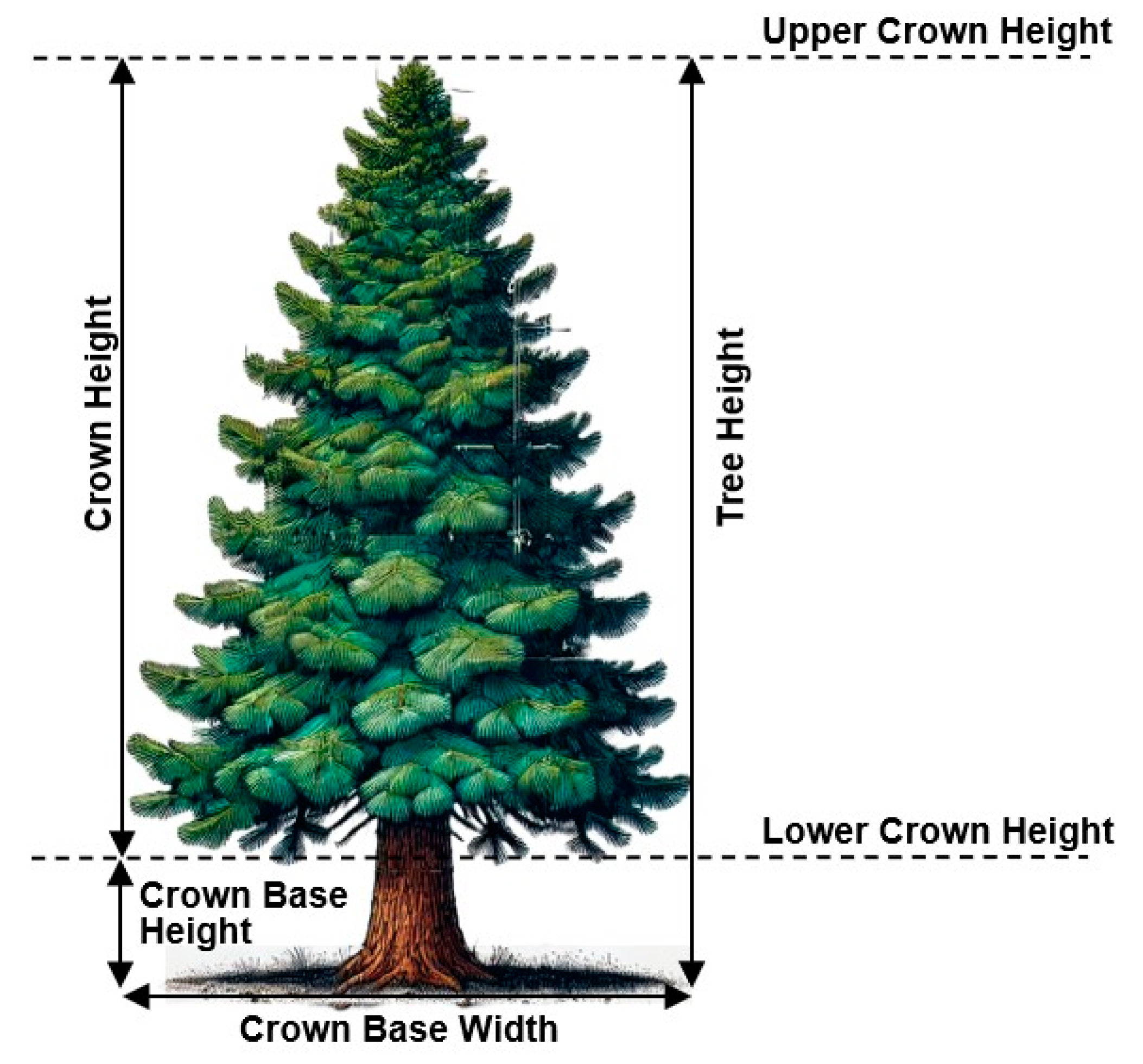
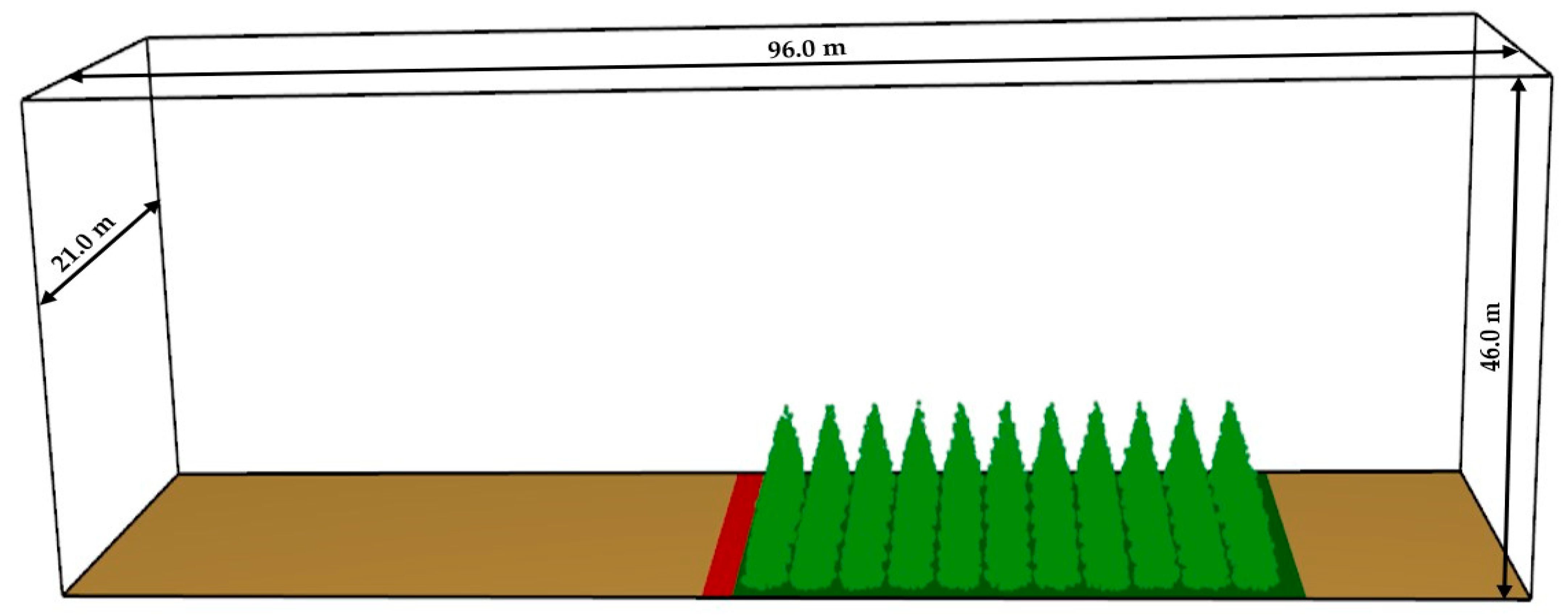
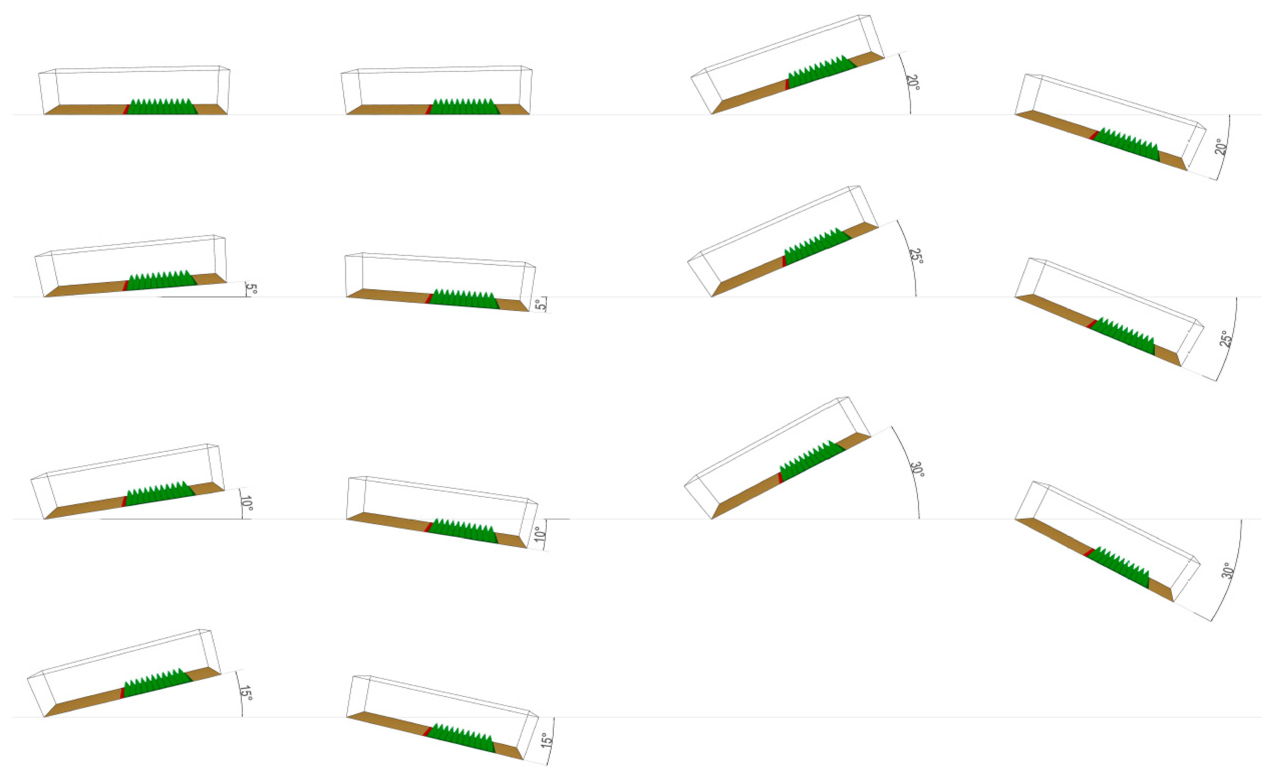
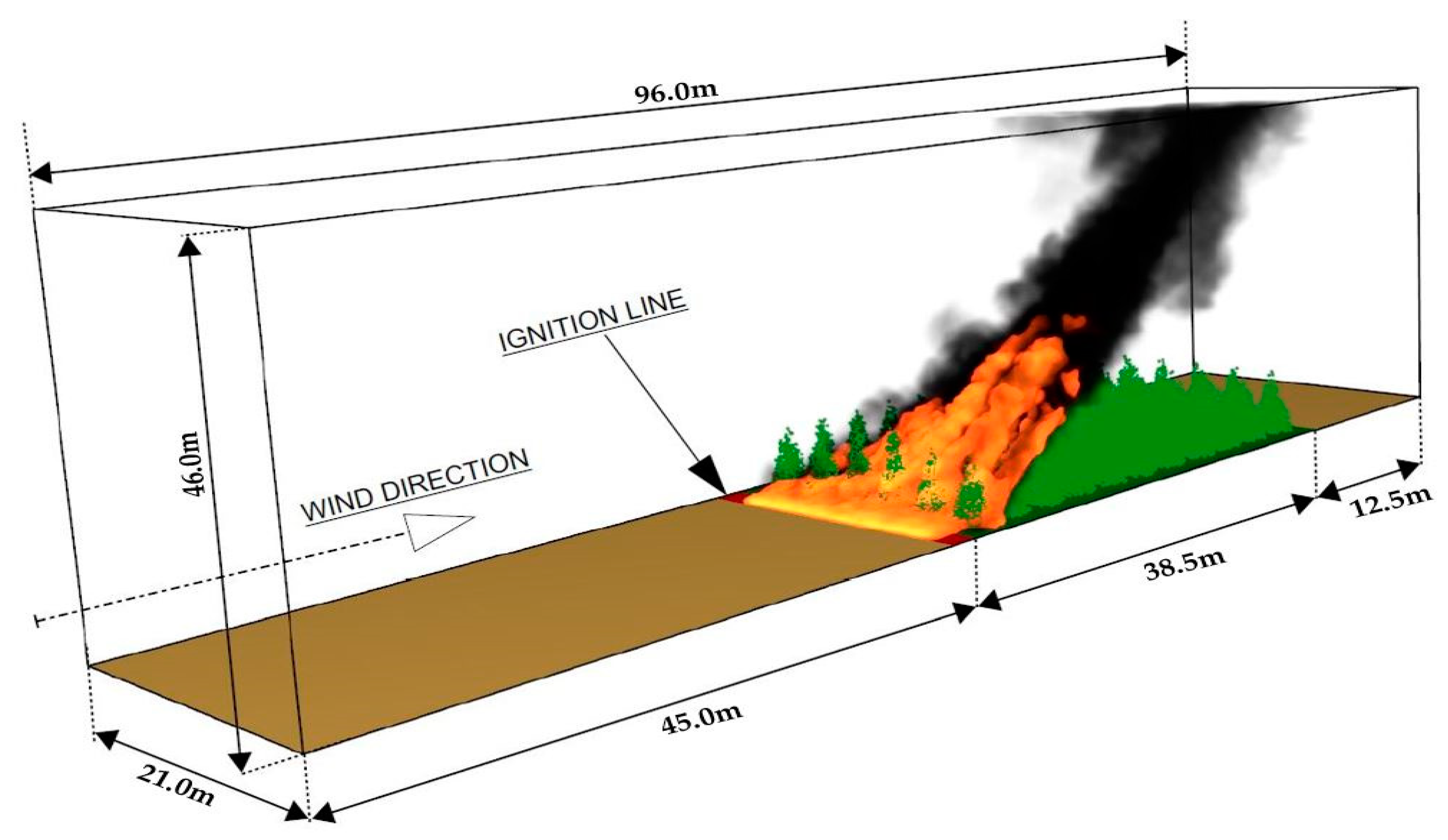
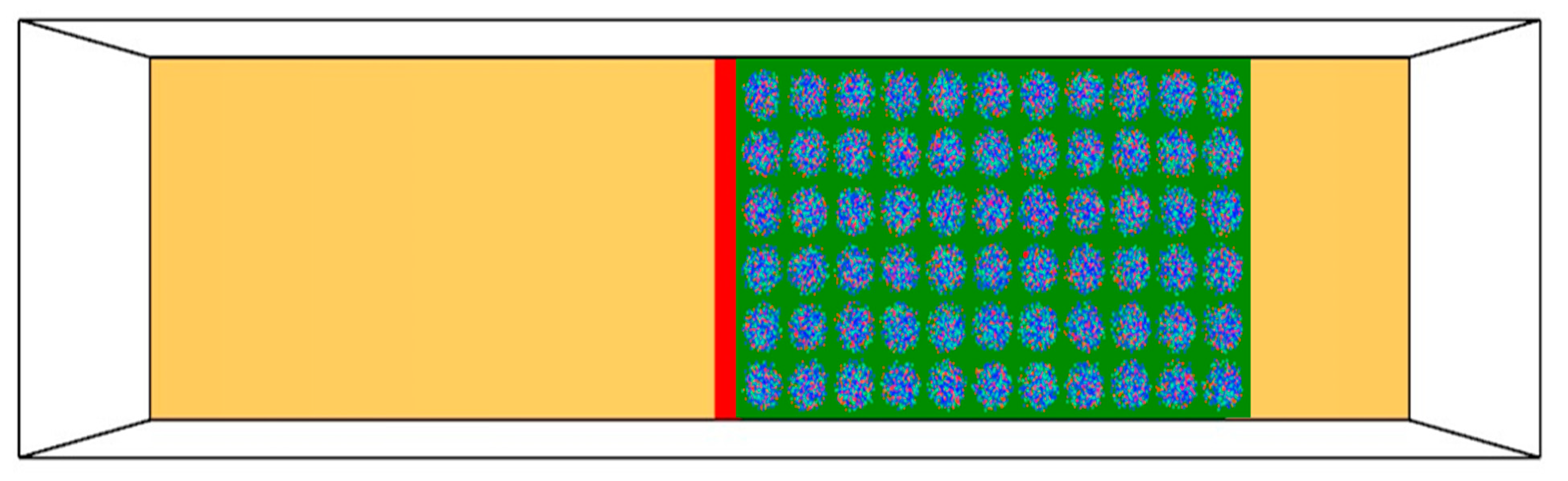
2. Model Characteristics and Plantation Setup

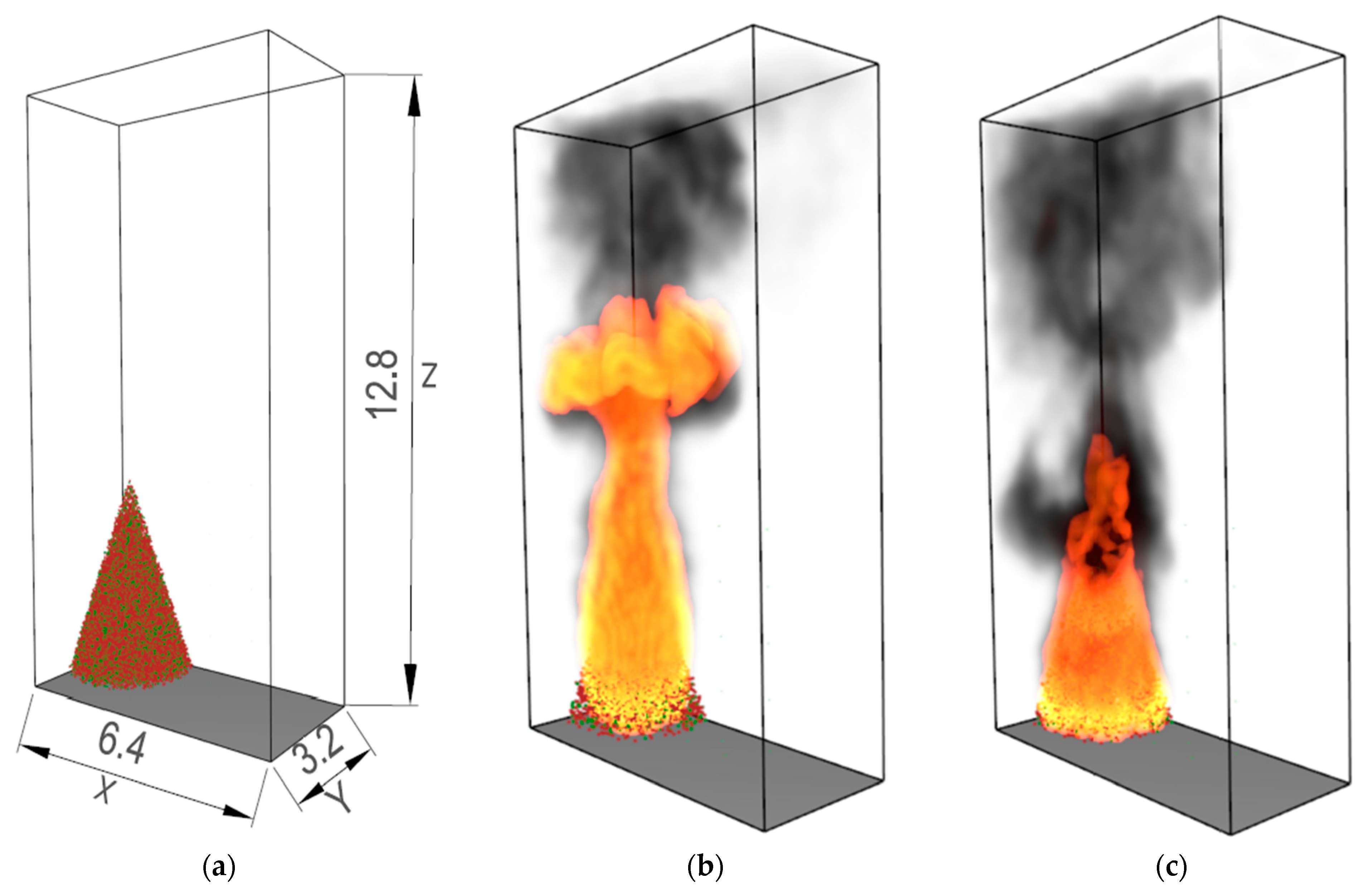
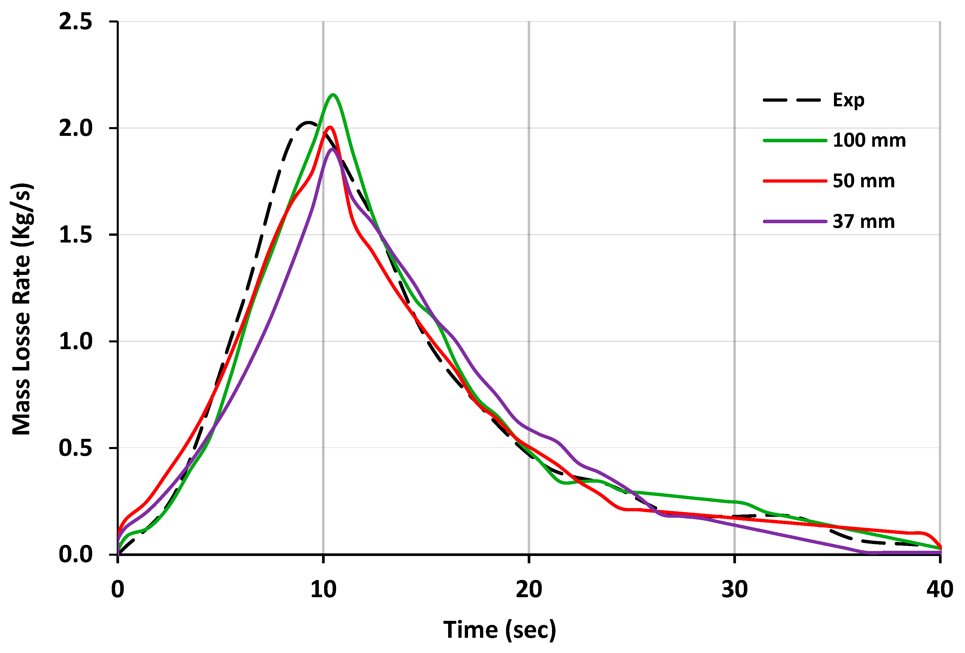
Figure 1 below illustrates the schematics and terminology used in the current study to present the Douglas Fir tree. This tree representation was chosen to follow the experiments conducted by [9], which showed good agreement with the CFD calculations. The key components of the Douglas Fir tree, including the crown, trunk, and base, are essential in understanding fire behavior. The crown consists of branches and foliage, while the trunk provides structural support, and the base influences ignition and fire spread. The main vegetation and fuel parameters used in numerical simulations are described in

Table 1. Vegetation and fuel parameters used in numerical simulations.

Parameter	Value	Units	Description
Vegetation Component Mass Densities
Foliage mass density	1.2336	kg/m3	Crown foliage distributed throughout tree cone
Small roundwood mass density	0.3495	kg/m3	Small-diameter branches and twigs
Medium roundwood mass density	0.2467	kg/m3	Medium-diameter branches
Large roundwood mass density	0.2262	kg/m3	Large-diameter branches and trunk components
Moisture Content
Foliage moisture fraction	0.26	-	Mass fraction of water in foliage (26%)
Roundwood moisture fraction	0.26	-	Mass fraction of water in all woody materials (26%)
Surface vegetation moisture fraction	0.063	-	Mass fraction of water in surface vegetation (6.3%)
Surface Area to Volume Ratios
Foliage	3940	m2/m3	High surface area characteristic of needles and leaves
Small roundwood	2667	m2/m3	Small-diameter woody fuels (≈0.5–1 cm)
Medium roundwood	888	m2/m3	Medium-diameter woody fuels (≈1–3 cm)
Large roundwood	500	m2/m3	Large-diameter woody fuels (≈3–5 cm)
Surface vegetation	9770	m2/m3	Ground-level fine fuels with high surface area
Thermal Properties
Heat of combustion	17,425	kJ/kg	Energy released during complete combustion
Thermal conductivity (vegetation)	2.0	W/m·K	Heat transfer coefficient within vegetation material
Thermal conductivity (char)	0.052	W/m·K	Heat transfer coefficient within char material
Thermal conductivity (ash)	0.1	W/m·K	Heat transfer coefficient within ash residue
Specific heat capacity	1.1–2.0	kJ/kg·K	Temperature-dependent: 1.1 at ambient temperature, increasing to 2.0 at 200–800 °C
Density (vegetation)	1000	kg/m3	Density of dry vegetation material
Density (char)	300	kg/m3	Density of char after pyrolysis
Density (ash)	67	kg/m3	Density of ash after char oxidation
Heat of reaction (pyrolysis)	418	kJ/kg	Energy required for thermal degradation of vegetation
Heat of reaction (char oxidation)	25,000	kJ/kg	Energy released during char combustion (exothermic)
Pyrolysis Parameters
Pre-exponential factor (vegetation)	1040	s−1	Arrhenius equation parameter for pyrolysis rate
Activation energy (vegetation)	61,041	J/mol	Energy barrier for pyrolysis reactions
Pre-exponential factor (char)	465	s−1	Arrhenius equation parameter for char oxidation
Activation energy (char)	68,000	J/mol	Energy barrier for char oxidation reactions
Mass fraction (char from vegetation)	0.25	-	Mass fraction of char produced during vegetation pyrolysis
Mass fraction (ash from char)	0.04	-	Mass fraction of ash produced during char oxidation
Drag coefficient	2.8	-	Air resistance coefficient through vegetation
Surface vegetation mass per volume	1.33	kg/m3	Density of ground-level vegetation layer

. The chemical composition of the vegetation fuel was modeled as C_2.10H_6.20O_2.16 with a soot yield of 0.01 representative of typical coniferous forest fuels based on the literature values [9]. The thermal degradation of vegetation was modeled using a two-step reaction scheme: (1) the pyrolysis of vegetation to produce fuel vapor and char and (2) the oxidation of char to produce ash. Both reactions were governed by Arrhenius-type kinetics with the parameters specified in Table 1. The specific heat capacities of the vegetation, char, and ash were implemented as temperature-dependent properties, increasing from 1.1 kJ/(kg·K) at ambient temperature to 2.0 kJ/(kg·K) at elevated temperatures (200–800 °C), accounting for the changes in thermal behavior of these materials during heating and combustion.

The moisture content values selected for a 5 m tall tree represent moderately dry conditions typical of fire seasons in temperate coniferous forests. The higher moisture content in the canopy (26%) compared to surface vegetation (6.3%) reflects the typical vertical moisture gradient observed in forest environments, where surface fuels dry more rapidly than canopy fuels, while, for 2 m tall tree, the average moisture content was 14% [9]. These moisture values significantly influence ignition thresholds, combustion rates, and overall fire spread behavior in our simulations.

Surface area to volume ratios were carefully selected to represent the different fuel size classes, with finer fuels (foliage and surface vegetation) having higher ratios that promote more rapid heating, drying, and ignition. These parameters directly affect the rate of heat transfer and, consequently, the fire spread rate through the forest stand.

The radiation heat transfer component is critical for the accurate prediction of wildland fire behavior, particularly for simulating fire spread across varied terrain. In our study, we implemented the radiation model embedded in the FDS, which uses a finite volume method to solve the radiative transport equation (RTE) [22]. This approach accounts for the complex interaction between radiation, combustion processes, and vegetation.

The radiation field is discretized using approximately 100 discrete solid angles, following the default angular discretization in FDS. This discretization has been previously validated for similar wildland fire applications [9,19] and provides sufficient accuracy while maintaining computational efficiency.

For the participating media radiation properties, we employed a combination of gas and soot radiation models. The radiative properties of combustion products (primarily CO₂ and H₂O) were calculated based on the specified fuel composition (C_2.10H_6.20O_2.16), while soot radiation was modeled using a soot yield parameter of 0.01 kg/kg, consistent with values reported for coniferous forest fuels [9]. The total absorption coefficient at each point in the domain was computed as the sum of contributions from both gaseous combustion products and soot, with the gas component calculated using the RadCal narrow-band model [6,23].

The adequacy of this radiation modeling approach was confirmed through our grid sensitivity analysis, which demonstrated convergence at 200 mm grid resolution for forest-scale simulations and 50 mm for single-tree simulations. The good agreement between our numerical results and experimental data for Douglas Fir combustion further validates the radiation model’s accuracy.

Two models were used to represent 66 trees. The first model consists of 66 trees with a height of 2.25 m, as described by Moinuddin, K.A., and Sutherland, D. [19]. Initially, the model’s dimensions included an enclosing box of 96 m in length, 25 m in height, and 8 m in width, with trees arranged in 16 or 17 rows and 4 columns, spaced 2 m apart. This model was validated against our study and, based on the validation, the tree arrangement was modified to 11 rows and 6 columns while maintaining the 2 m spacing between trees. The adjustment was made as changes to the model’s width do not significantly impact the capture of essential eddies, flame lengths in the lateral direction, or HRR [19]. This adjustment was made to facilitate a comparison between model 1 (66 trees at 2.25 m height) and model 2 (66 trees at 5 m height).

The second model represents a plantation of 66 trees with a height of 4.6 m, consisting of a crown base height of 0.3 m, a crown height of 4.3 m, and a crown base width of 2.9 m. Figure 1 illustrates the definitions of these physical dimensions. The tree dimensions were selected based on experimental data [9]. Consequently, the overall model dimensions were adjusted to 96 m in length, 50 m in height, and 21 m in width. Figure 2 depicts the plantation layout for the 5 m tree model on a zero-slope surface. To ensure consistency in the comparison, the spacing between trees in Model 2 was proportionally increased. In Model 1, the spacing between trees was set to 2.0 m, while in Model 2, the spacing was adjusted to 3.5 m to maintain the same relative separation relative to the 5 m tree dimensions. Additionally, the placement of the ignition line and tree positions in the 5 m plantation model were aligned with those in the 2 m plantation model. In this study, the 2.25 m and 4.6 m tree heights are equivalent to the 2 m and 5 m tree heights, respectively, as indicated in [9].

3. Numerical Model

FDS is a CFD tool specifically designed to handle wildlife fires using the large eddy simulation approach (LES). The flow is assumed to be compressible and the low Mach number approximations are used. The complete mathematical description of FDS can be found in references [23,24,25]; however, some of the main governing equations of the code are presented in this article. The mass and momentum balance equations solved in the simulation are as follows.

The following mass conservation equation links the variation of the density $\rho$ to the velocity field $u$.

$${\displaystyle \frac{\partial \overline{p}}{\partial t}}+{\displaystyle \frac{\partial \overline{\rho }\widetilde{u_i}}{\partial x_i}}=0$$

(4)

The following momentum conservation equation allows us to solve the pressure field p:

$${\displaystyle \frac{\partial \overline{\rho }\widetilde{u_i}}{\partial t}}+{\displaystyle \frac{\partial }{\partial x_j}}\left(\overline{\rho }\widetilde{u_i}\widetilde{u_j}\right)=-{\displaystyle \frac{\partial \overline{p}}{\partial x_i}}+{\displaystyle \frac{\partial \overline{{\mathrm{\Omega }}_{ij}}}{\partial x_j}}-\partial {\tau }_{ij}^{*}+f_b+\overline{\rho }{g}_i$$

(5)

where ${\tau }^{*}$ is the LES subgrid scale stress tensor (Deardoff model is used in this model [23]) and $f_b$ is the external force vector applied to the domain.

The viscous stress can be written as a function of the bulk viscosity ${\mu }_B$ (zero in the case of massless particles):

$${\mathrm{\Omega }}_{ij}=2\mu \left(S_{ij}-{\displaystyle \frac{1}{3}}{\delta }_{ij}{S}_{kk}\right)+{\mu }_B{\delta }_{ij}{S}_{kk}$$

(6)

where the rate of strain is $S_{ij}={\displaystyle \frac{1}{2}}\left({\displaystyle \frac{\partial u_i}{\partial x_j}}+{\displaystyle \frac{\partial u_j}{\partial x_i}}\right)$ along directions I and j.

The Poisson equation gives information on the total pressure $H={\displaystyle \frac{\left|{\tilde{u}}^2\right|}{2}}-{\displaystyle \frac{\overline{p}}{\overline{\rho }}}$ field and, therefore, the temperature.

$${\nabla }^{2}H=-{\displaystyle \frac{\partial \left(\nabla .\tilde{u}\right)}{\partial t}}-\nabla .F$$

(7)

With the momentum flux $F=-\tilde{u}\times \omega -\overline{p}\nabla \left({\displaystyle \frac{1}{\overline{\rho }}}\right)-\left({\displaystyle \frac{1}{\overline{\rho }}}\right)\left[\left(\overline{\rho }-{\rho }_0\right)g+f_b+\nabla .{\tau }_{ij}^{*}\right]$, $\omega$ is the flow vorticity and ${\rho }_0$ is the density at the initial temperature.

The following ideal gas equation also applies to our case.

$${\displaystyle \frac{\overline{p}}{\overline{\rho }}}={\displaystyle \frac{R}{\overline{W}}}\tilde{T}$$

(8)

In this equation, R is the universal gas constant and $\overline{W}$ is the Reynolds filtered molecular weight (here taken as the value for standard air). The third Navier–Stokes equation is the energy balance formula:

$${\displaystyle \frac{\partial \left(\overline{\rho }{C}_p\tilde{T}\right)}{\partial t}}+\nabla .\left(\overline{\rho }\tilde{u}{C}_p\tilde{T}-{\displaystyle \frac{\overline{\rho }{\mu }_t{C}_p}{P{r}_t}}\tilde{T}\right)={\displaystyle \frac{D\left(\overline{p}\right)}{Dt}}-\nabla .{\tilde{q}}^{″}$$

(9)

where $C_p$ is the specific heat of the gas at constant pressure, $P{r}_t={\displaystyle \frac{\nu }{\alpha }}$ is the turbulent Prandtl number (ratio of the momentum diffusivity $\nu$ and the thermal diffusivity $\alpha$), and ${\mu }_t$ is the turbulent (subgrid) viscosity, which is used with the specific heat and the turbulent Prandtl number to calculate the thermal conductivity. $\nabla .{\tilde{q}}^{″}$ is the term representing radiative heat loss, which is calculated by solving a radiative transport equation.

It is assumed that the temperature and density variations are large, and the pressure variation is negligible. As the combustion gas consists of a mixture of species (e.g., carbon dioxide, dioxygen, water vapor), it is necessary to solve transport equations for each species. The species equation used in the code is given below:

$${\displaystyle \frac{\partial \left(\rho Y_k\right)}{\partial t}}+\nabla .\left(\rho \mathit{u}{Y}_k\right)=\nabla .\left(\rho D_k\nabla Y_k\right)+{\dot{W}}_k^{‴}$$

(10)

where $Y_k$ is the mass fraction of the kth species, $D_k$ is the diffusion coefficient of species k into the mixture, u is the velocity vector (u1, u2, u3), and $W_k$ is the production rate of the species k.

The numerical tools used in this study are capable of not only modelling the fire spread through trees, but also to covering other situations such as grasses, understory growth, and litter that can, if needed, make our model even more realistic.

Another feature of this particular CFD tool is to model the thermal degradation of the vegetation, i.e., the loss of mass by the tree through water evaporation (fuel drying) and pyrolysis processes. For instance, at the lower temperature T = 373 K, the water evaporation is modelled using the following approximation:

$${\dot{m}}_{vap}={\displaystyle \frac{{\dot{Q}}_{net}}{\mathrm{\Delta }{h}_{vap}}}$$

(11)

where the vegetation surface temperature $T_s=373 K$, ${\dot{m}}_{vap}$ is the MLR through evaporation, ${\dot{Q}}_{net}$ is the net energy through convection and radiation on the fuel surface, and $\mathrm{\Delta }{h}_{vap}$ is the latent heat of evaporation. As described in [26], the pyrolysis begins once the water has entirely evaporated and the temperature reaches 400 K. Between 400 K and 500 K, the following model is used.

$${\dot{m}}_{pyr}={\displaystyle \frac{{\dot{Q}}_{net}}{\mathrm{\Delta }{h}_{pyr}}} {\displaystyle \frac{T_s-400}{500-400}}$$

(12)

${\dot{m}}_{pyr}$ is the pyrolysis rate and $\mathrm{\Delta }{h}_{pyr}$ is the heat of reaction.

The variation of surface temperature is itself calculated using the heat balance equation below.

$${\overline{\rho }}_s{C}_s{\displaystyle \frac{d{T}_s}{dt}}=D{\displaystyle \frac{{\partial }^2{T}_s}{\partial x^2}}+h\left(T-T_s\right)+{\varphi }_{Fl\to s}$$

(13)

${\overline{\rho }}_s$ is the vegetation bulk density, $C_s$ is the specific heat capacity, and h is the convective heat transfer coefficient. D is the vegetation thermal diffusivity. $Q_{Fl\to s}$ is the radiant heat energy on the fuel surface. It is calculated using the ray-tracing method from advancing flame temperature:

$$Q_{Fl\to s}={\displaystyle \frac{{\alpha }_s{\sigma }_s}{4}} \left( J-4\sigma T_s^4\right)$$

(14)

where J is the total irradiance calculated from the radiative transport equation, $\sigma$ is the Stefan constant, ${\sigma }_s$ is the surface-to-volume ratio, and ${\alpha }_s$ is the vegetation packing ratio.

The char oxidation is not accounted for in this simulation as it occurs at higher temperatures. The speed of reaction in FDS can be modelled using the following Arrhenius formula.

$$k=A\times \exp \left(-{\displaystyle \frac{E_a}{RT}}\right)$$

(15)

k is the reaction rate, T is the absolute temperature, A is the frequency factor, R is the universal gas constant, and $E_a$ is the activation energy. The FDS tool uses the mixing–controlling combustion model to calculate the chemical reaction as described in [23].

4. Results and Analysis

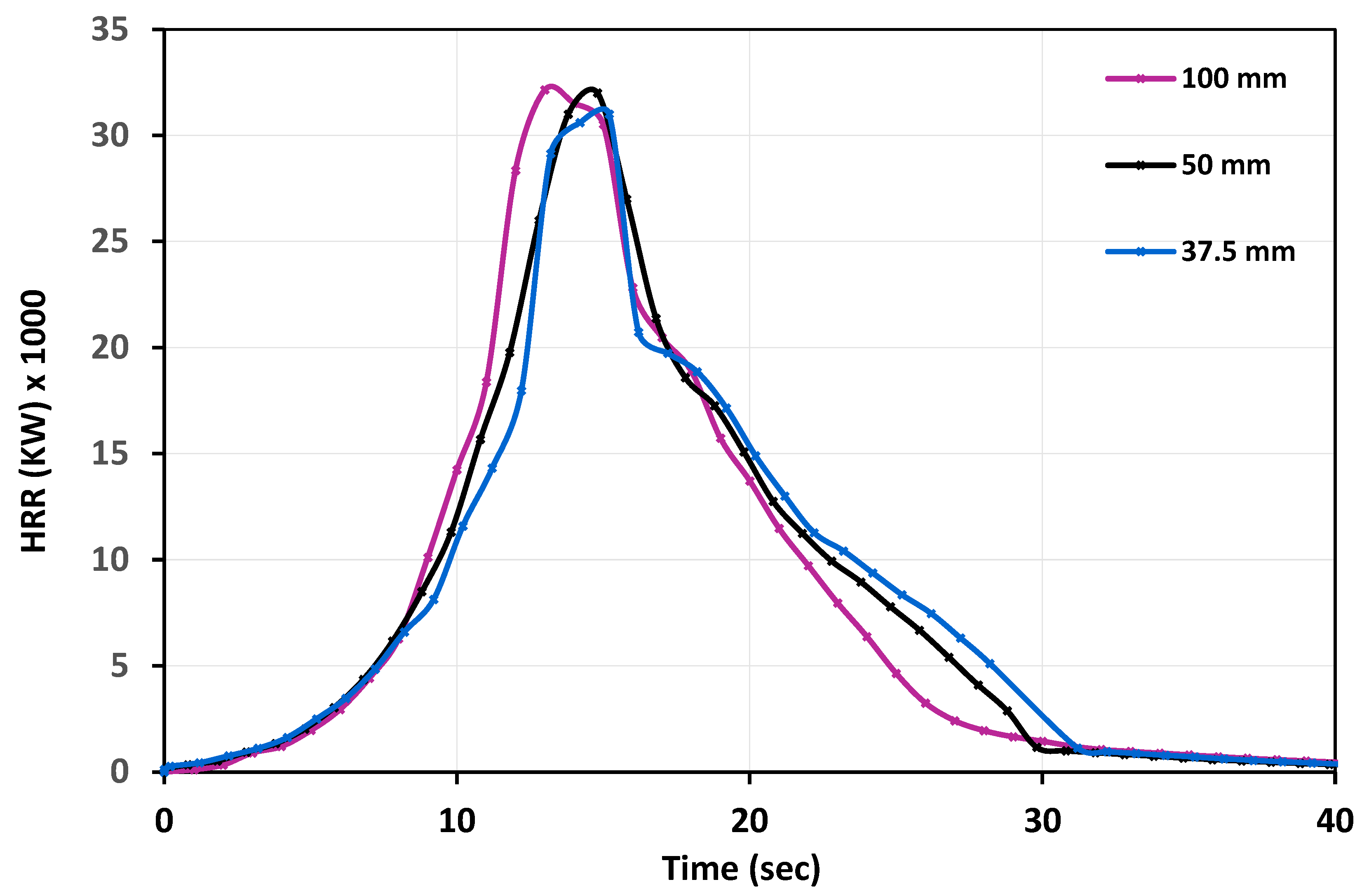
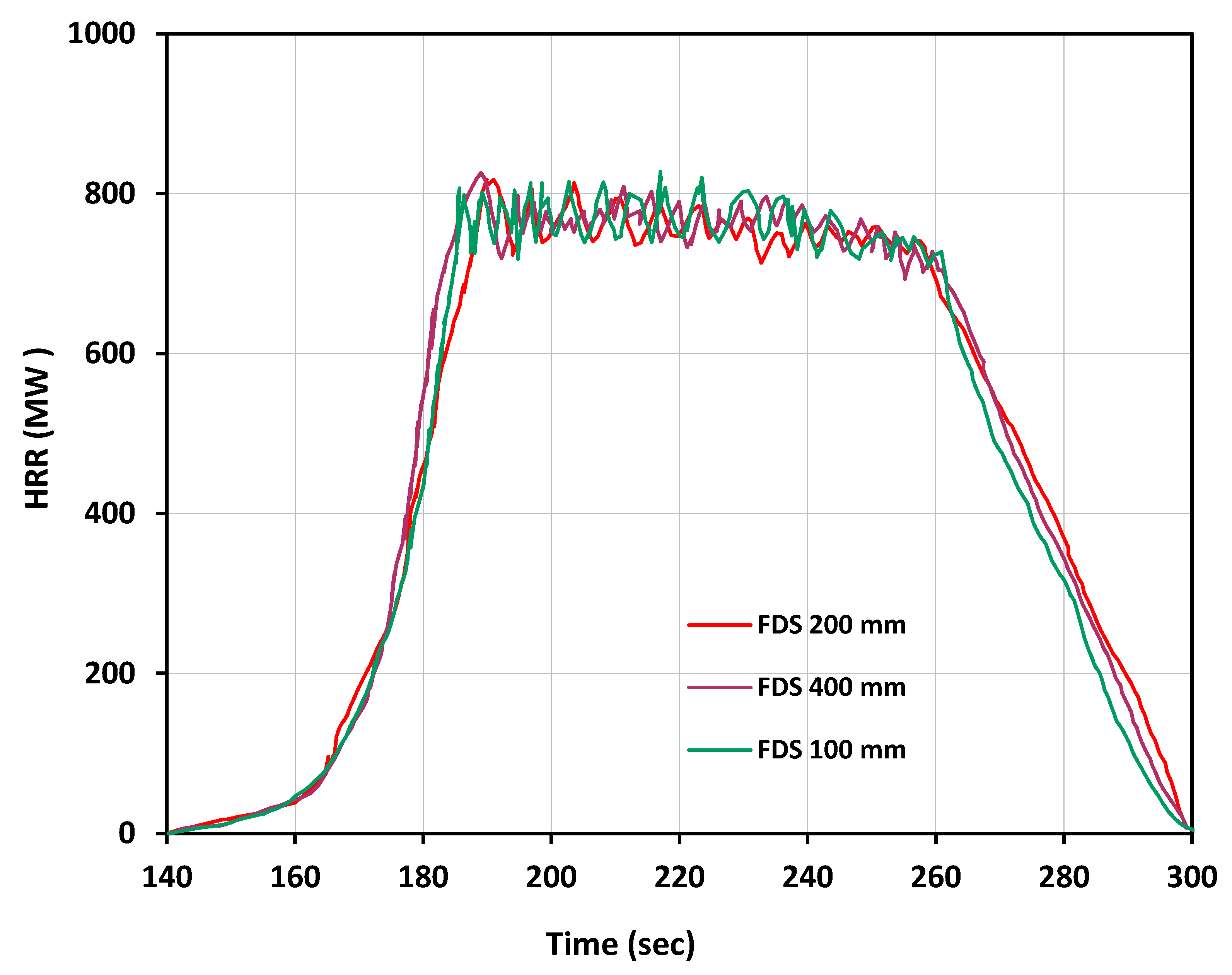
4.1. Simulation of 5 m Douglas

In the first step of this study, a single Douglas Fir tree was simulated using the FDS tool incorporating the governing equations described in the previous section. The height of the tree is 4.6 m. Figure 3 illustrates the model dimensions. The numerical simulations were carried out using the OzSTAR supercomputing facility at Swinburne University, which provides advanced computational resources to researchers. The grid cell sizes used in FDS were 100 mm, 50 mm, and 37.5 mm, resulting in total cell counts of 262,144, 2,097,152, and 3,816,336, respectively.

Figure 3 presents (a) the computational domain dimensions (6.4 × 3.2 × 12.8 m) used for simulating the 5 m single Douglas Fir tree, and (b) and (c) the progression of fire at different time points following ignition. These simulations demonstrate the characteristic bottom-to-top fire spread pattern typically observed in wildland fires, driven by buoyant convection. The upward flame propagation corresponds to the temperature contours shown in Figure 4, where gas-phase temperatures reach up to 1550 °C in the crown region. This visualization aligns with the mass loss rate and heat release rate data presented in Figure 5 and Figure 6, showing the progression from ignition to peak combustion (around 10–15 s) and subsequent decline as fuel is consumed. The FDS model effectively captures the complex physical processes involved, including moisture evaporation, the pyrolysis of vegetation to produce fuel vapor and char, and the subsequent oxidation reactions governed by the Arrhenius-type kinetics detailed in Section 2. The grid sensitivity analysis (50 mm resolution) provides sufficient detail to accurately represent these combustion dynamics while maintaining computational efficiency.

Figure 4 presents CFD visualizations of the characteristic burning stages of a single Douglas Fir tree. These results align well with the findings of Mell et al. [9], which focused on a smaller tree. However, the 21 s simulation duration is insufficient to capture the full thermal degradation of the tree, as a 61 s period was required for a smaller tree in the referenced study. The simulation shows temperatures reaching 800 °C at 5 m above the tree, with a peak temperature of 1550 °C observed in the canopy.

Figure 5 presents the grid independence study, where three different structured grid sizes were tested in the initial FDS simulations. Mass loss and HRR were selected as key metrics for determining the optimal mesh size, as they are the most relevant parameters for comparison with the laboratory measurements from [9]. This step is crucial in ensuring computational accuracy, as excessively coarse grids can lead to inaccurate results, while overly fine meshes significantly increase computational time. The selected inputs demonstrated good agreement between the experimental data and CFD calculations, with similar mass loss behavior across the three mesh sizes and a strong correlation with experimental results. Figure 6 illustrates the HRR curves, showing a strong correlation across different mesh sizes, except for the coarsest 100 mm grid, which deviates significantly. Based on these findings, a 50 mm mesh was selected for further simulations to balance accuracy and computational efficiency. For validation, Mell et al. [9] reported a peak HRR of approximately 28 MW for a 5 m tree.

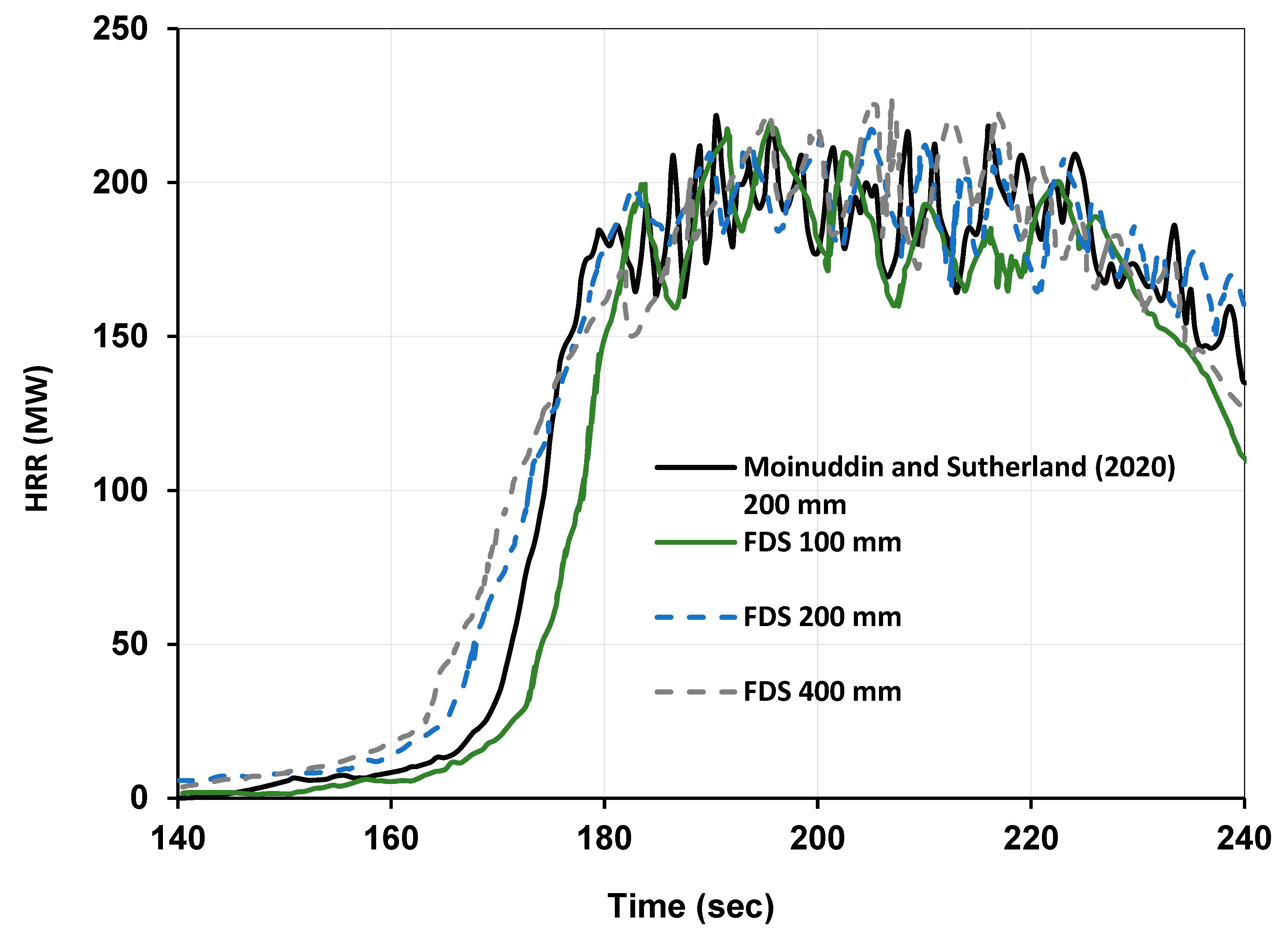
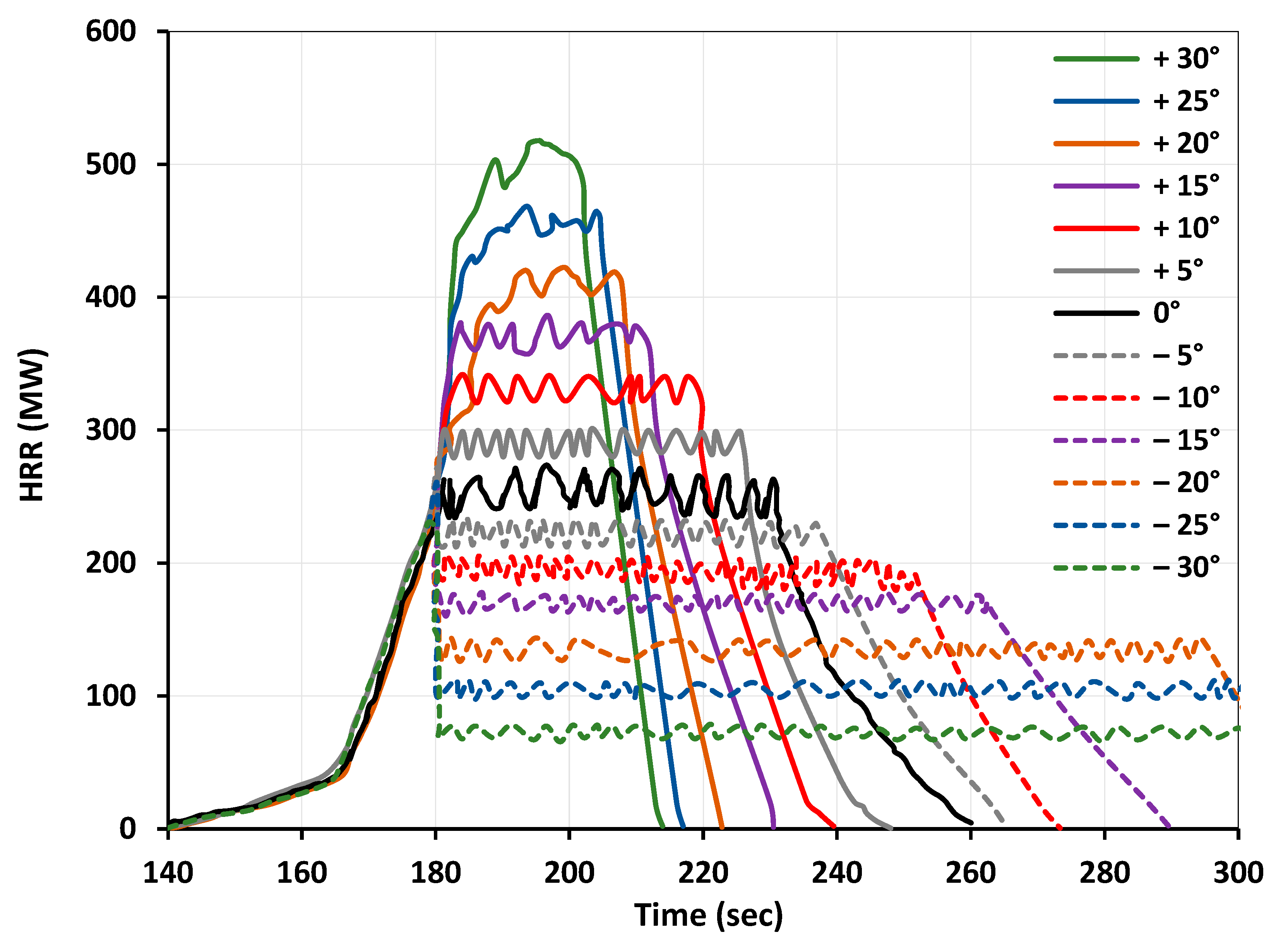
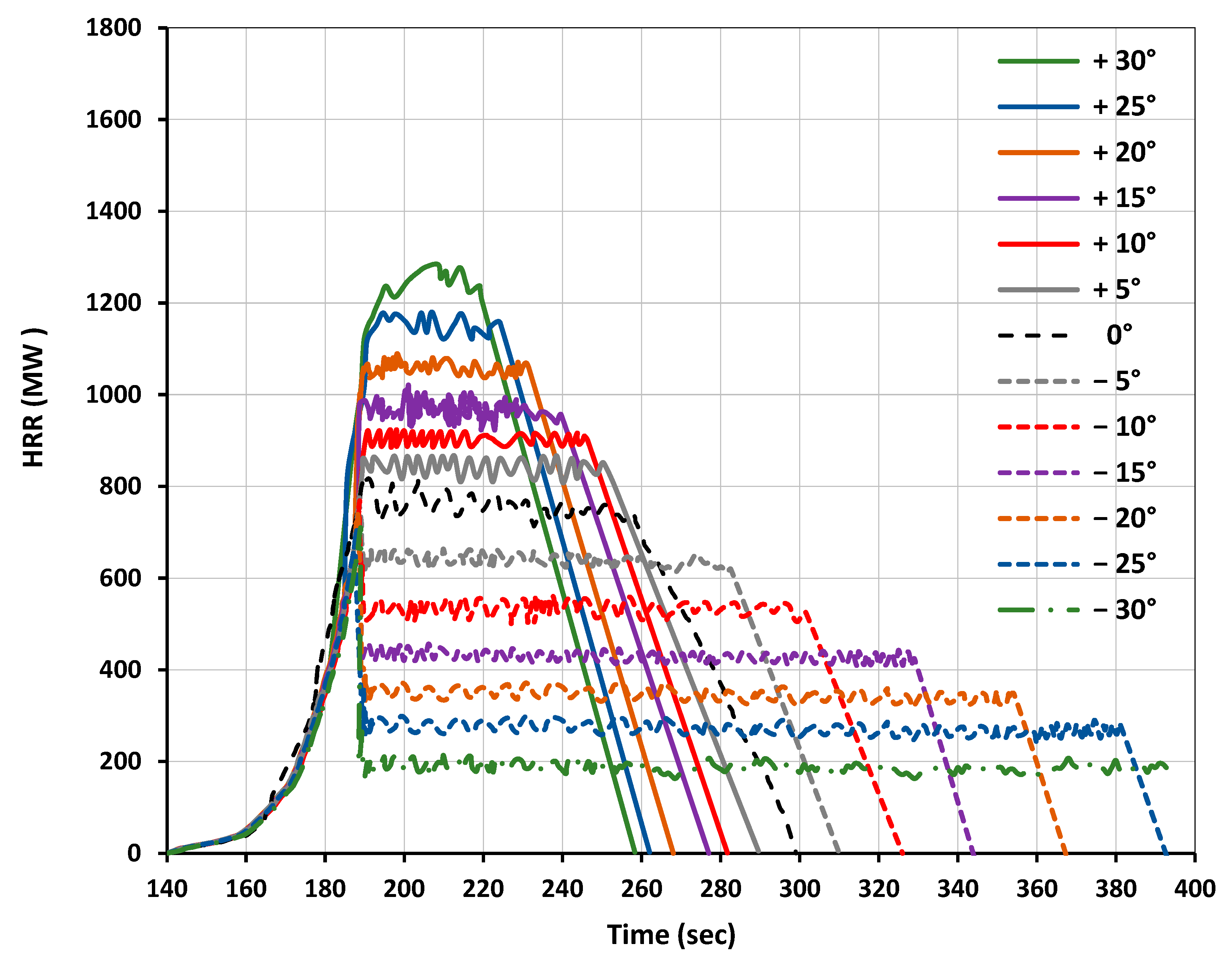
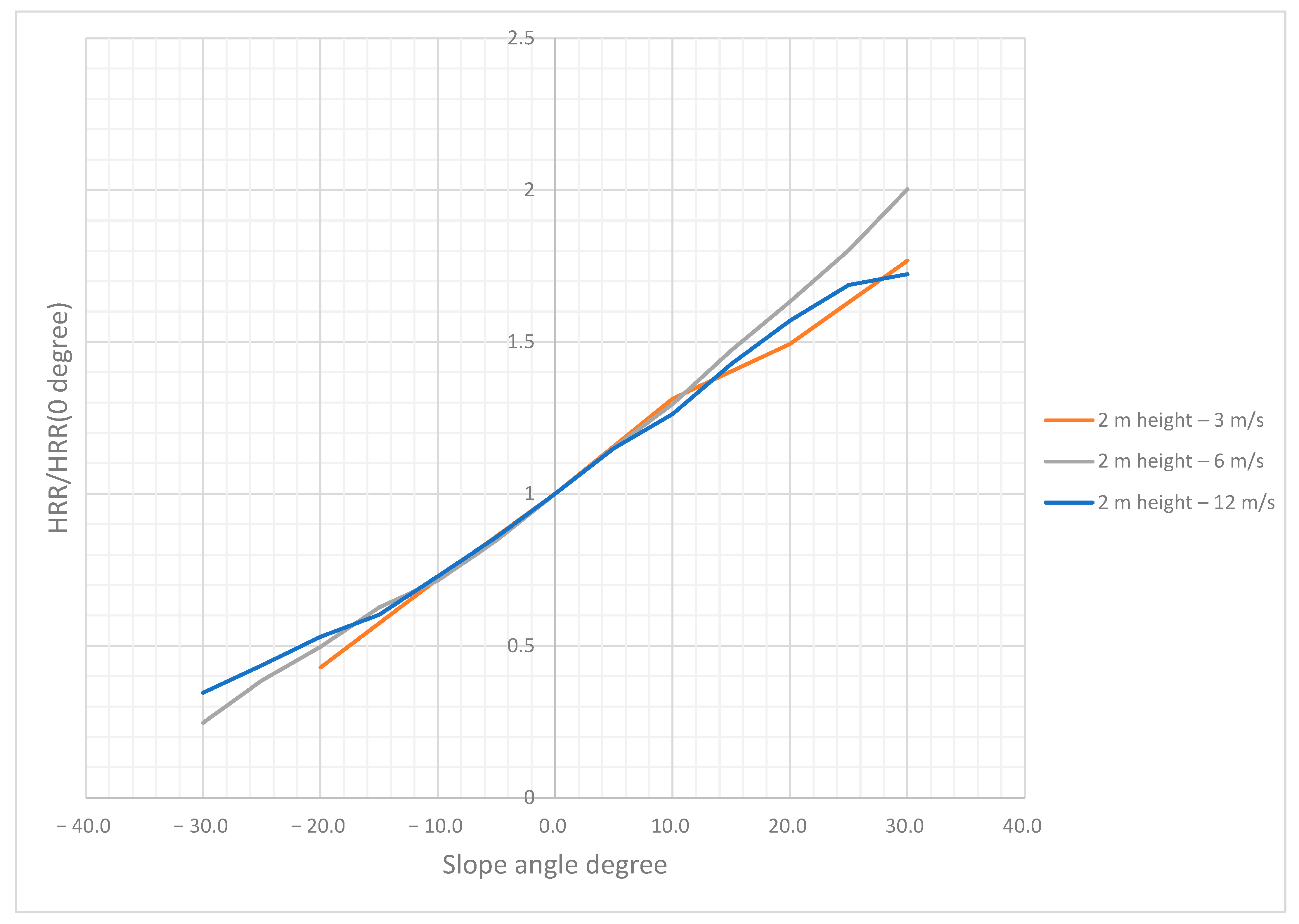
4.2. Simulation of 66 Douglas Fir Trees (2 m)

This section presents and analyzes the simulations conducted by Moinuddin, K.A., and Sutherland, D. [19], where a 2 m high Douglas Fir tree was modeled. Their study examined both a single tree and a plantation of 66 Douglas Fir trees. To validate the present model, a plantation of 66 trees was initially simulated on a flat (zero-slope) surface and compared against the results of [19]. Following validation, additional simulations were conducted across a range of slopes from −30° to +30° in 5° increments to investigate the influence of terrain on fire behavior.

Figure 7 provides a visual representation of slope configurations. While this study considers a defined plantation area, previous research by Balbi et al. [4] introduced a numerical methodology for tracking large-scale topographic changes. Their approach suggests the potential for extending this research to cover larger land areas with more complex and varied topography. To validate the model and perform grid convergence testing, three models with grid sizes of 100 mm, 200 mm, and 400 mm were compared with the simulation results from Moinuddin, K.A., and Sutherland [19] at a 200 mm grid cell size. It can be seen that the 200 mm grid results for the current study and [19] are in good agreement, indicating that convergence in the model was achieved with a 200 mm grid size. Figure 8 shows good agreement results of the mesh independence study.

In the first part of the tree plantation simulation, it was decided that the wind was allowed to travel through the domain at 2.5 travel time in order to develop its velocity field fully before the actual tree ignition starts. The rationale was developed through a trial-and-error method by [19] and consists in establishing the flow turbulence level as well as the velocity profile. The wind speed acts horizontally (parallel to the x-axis) throughout the domain. We implemented a 1/7th power law model [27] of the atmospheric boundary layer prescribed at the domain inlet, with an inlet boundary wind speed specified as 3 m/s at 2 m height. This wind speed varies with height following the atmospheric boundary layer model rather than being constant over the entire height, with velocity profiles following a logarithmic relationship with height [28] for a detailed explanation.

After the air velocity field is fully established, a 1000 mm deep ignition line across the whole domain width with 500 kW/m² HRR per unit area was activated for 5 s to ignite the fire and to allow it to spread to the tree crowns. While local variations in wind speed occur due to the presence of trees and the developing fire, the background wind field remains consistent from the first to the last tree, subject only to the natural turbulent fluctuations that would be expected in a forest environment. It can also be noted that, as the domain measures 96 m long, 140 s would allow for the establishment of a cold flow field with wind speeds of 3 m/s at 2 m high.

In this simulation, the fire inception occurs at 140 s, then reaches the steady state at about 180 s until 220 s. The steady state itself presents fluctuations of about +/−10% of the mean HRR value. It can be observed on this diagram that the grid size of 200 mm seems to offer a good trade-off between computation time and HRR prediction accuracy. The overall heat produced exceeds 200 MW for the plantation.

The next step of the study consists of running a number of CFD cases covering several wind speeds (3 m/s, 6 m/s, 12 m/s) and a number of slopes ranging from −30° to +30° by steps of 5° up to 13 slopes per wind speed in total. For all of the calculations, the combustion inception occurs at the same moment of 140 s and the fire spread on the first range of trees occurs in a very similar way independently from the slope and the wind speed value. Figure 9, Figure 10 and Figure 11 show the HRR characteristics of the different cases covered.

Figure 9, Figure 10 and Figure 11 illustrate the HRR for wind speeds of 3 m/s, 6 m/s, and 12 m/s, respectively. Wind speed plays a crucial role in fire spread rate and significantly influences the shape of the HRR curve [29]. As previously mentioned, fire inception occurs similarly across all cases, with each case reaching a steady state in the ROS and HRR at approximately 80 s. The value demonstrated by negative slopes are below the peak HRR value achieved at 180 s; however, the duration of the combustion reaction is longer. The surface area below the curve stays constant for each slope and corresponds to the amount of energy enclosed in the tree plantation. On the other side, positive slopes demonstrate higher peak values of the HRR, but the combustion lasts for a relatively short time. The fluctuations observed around the average value of HRR during the steady combustion phase usually do not exceed +/−10%, as was observed during the grid independence study calculation in Figure 8. The analysis of the average steady combustion phase HRR value against the zero-slope reference value will be conducted later in this article.

In terms of the comparison between different wind speeds, the higher 12 m/s value demonstrates approximately a 30% increase in the HRR amplitude, while the lower 3 m/s speed results in roughly a 30% decrease in the HRR amplitude compared to the average 6 m/s. The findings from these simulations contribute to establishing a mathematical correlation model, as explained in Section 4.4.

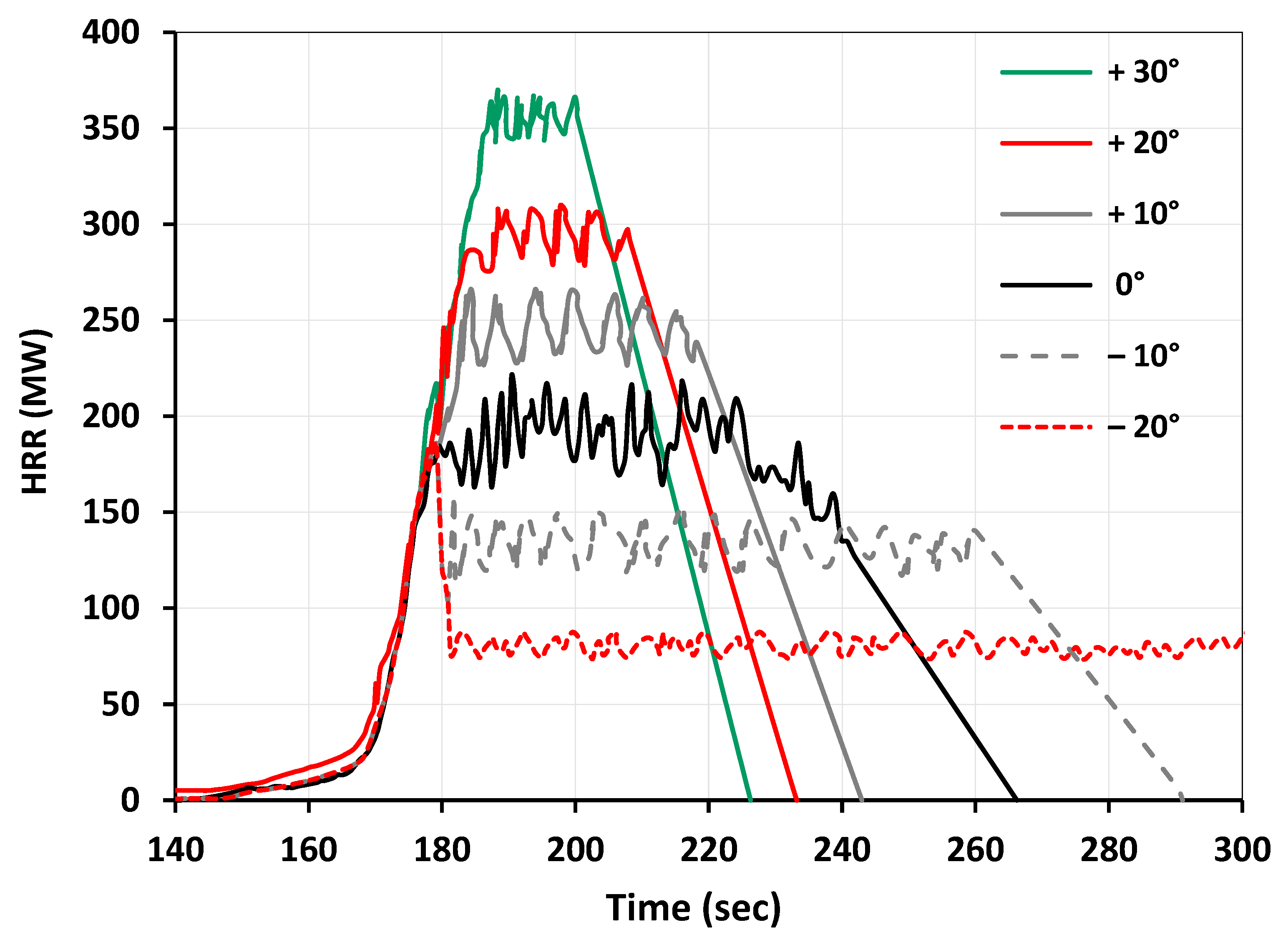
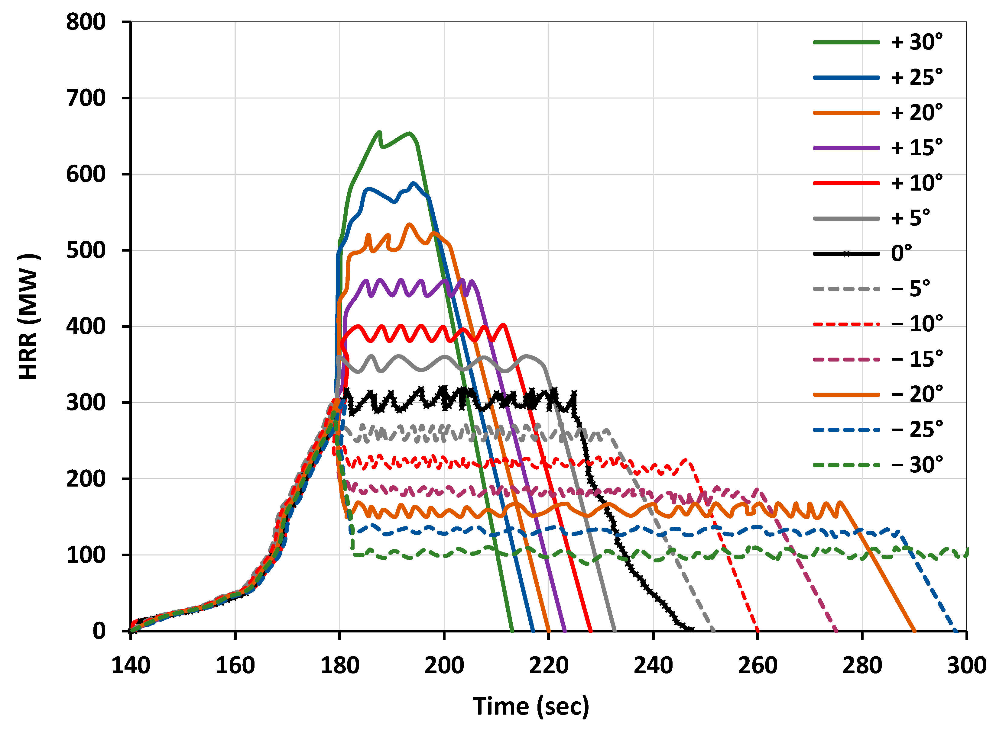
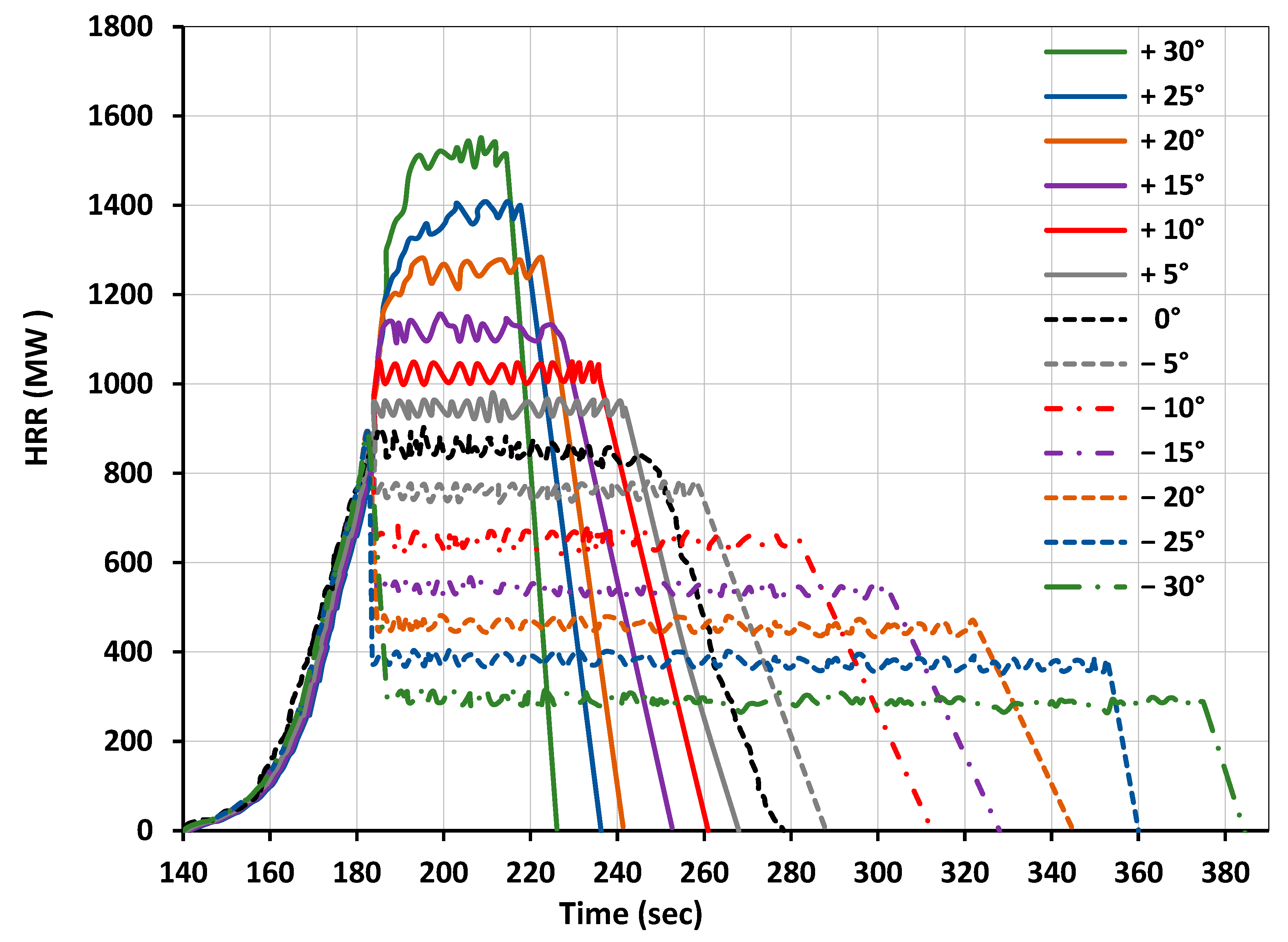
4.3. Simulation of 66 Douglas Fir Trees (5 m)

The study domain, as depicted in Figure 12 and Figure 14, includes a plantation organized in a grid configuration of 11 rows and 6 columns, with 66 trees spaced 3.5 m apart both between columns and individual trees. Figure 13 captures a snapshot of the burning plantation at t = 180 s, depicting the quasi-steady flame propagation as the HRR fluctuates near its maximum value. Also, the figure demonstrates the fire’s behavior at its peak intensity, with flames spreading steadily but with slight variations in HRR due to the complex interactions between the fire, wind, and tree canopy; as shown in Figure 15, the quasi-steady period extends from t = 180 s to t = 260 s.

According to [19], no additional space on the sides of the plantation is required. The inlet boundary wind speed is set at 3 m/s, 6 m/s, or 12 m/s at a height of 2 m. Once the wind field is established, a 1 m deep ignition line spanning the entire width of the domain is activated for 5 s to initiate the fire, with a HRR of 500 kW/m². In these simulations, the domain height is set to 10 times the height of the canopy, which consists of 5 m tall trees. Shorter downstream distances within the domain have been observed to lead to lower HRR, with apparent convergence occurring at reduced domain heights. It is crucial that the domain is large enough to allow the fire to grow naturally; if the domain is too small, the HRR may be artificially limited, potentially leading to inaccurate simulation results.

The grid size independence study for this domain is illustrated in Figure 15. The study was conducted by simulating a reference case with a 0° slope and minimum wind speed 3 m/s. The results demonstrate nearly identical HRR amplitudes across all time steps, confirming grid independence. A grid size of 200 mm was selected, as it offers an optimal balance between computational accuracy, efficiency, and calculation speed.

The graphs in Figure 16, Figure 17 and Figure 18 depict curves equivalent to those previously shown in Figure 9, Figure 10 and Figure 11. The fire inception time remains at 140 s, with the steady-state regime beginning at 180 s. However, compared to the 2 m tree height plantation case, the variation in HRR amplitudes across different wind speeds is lower, not exceeding 20% between 12 m/s and 6 m/s, as well as between 6 m/s and 3 m/s.

The small fluctuations occurring during the steady-state regime are also lower in amplitude relative to the mean value compared to the 2 m tree height calculations. The overall behavior remains very similar to the 2 m tree height plantation, with the main conclusions still holding: the same fire inception pattern, the same area under the curves, and higher peaks with quicker burnout times for higher slope values. However, it is important to determine the average values of steady-state HRR amplitudes to investigate the effects of slope and wind speed on the HRR/HRR(zero slope) metric. This analysis will be presented in the next section, aiming to establish a reduced-order model comparable to those proposed by [10,12,13] and other researchers, but based on LES CFD calculations, ensuring full control over all computational parameters.

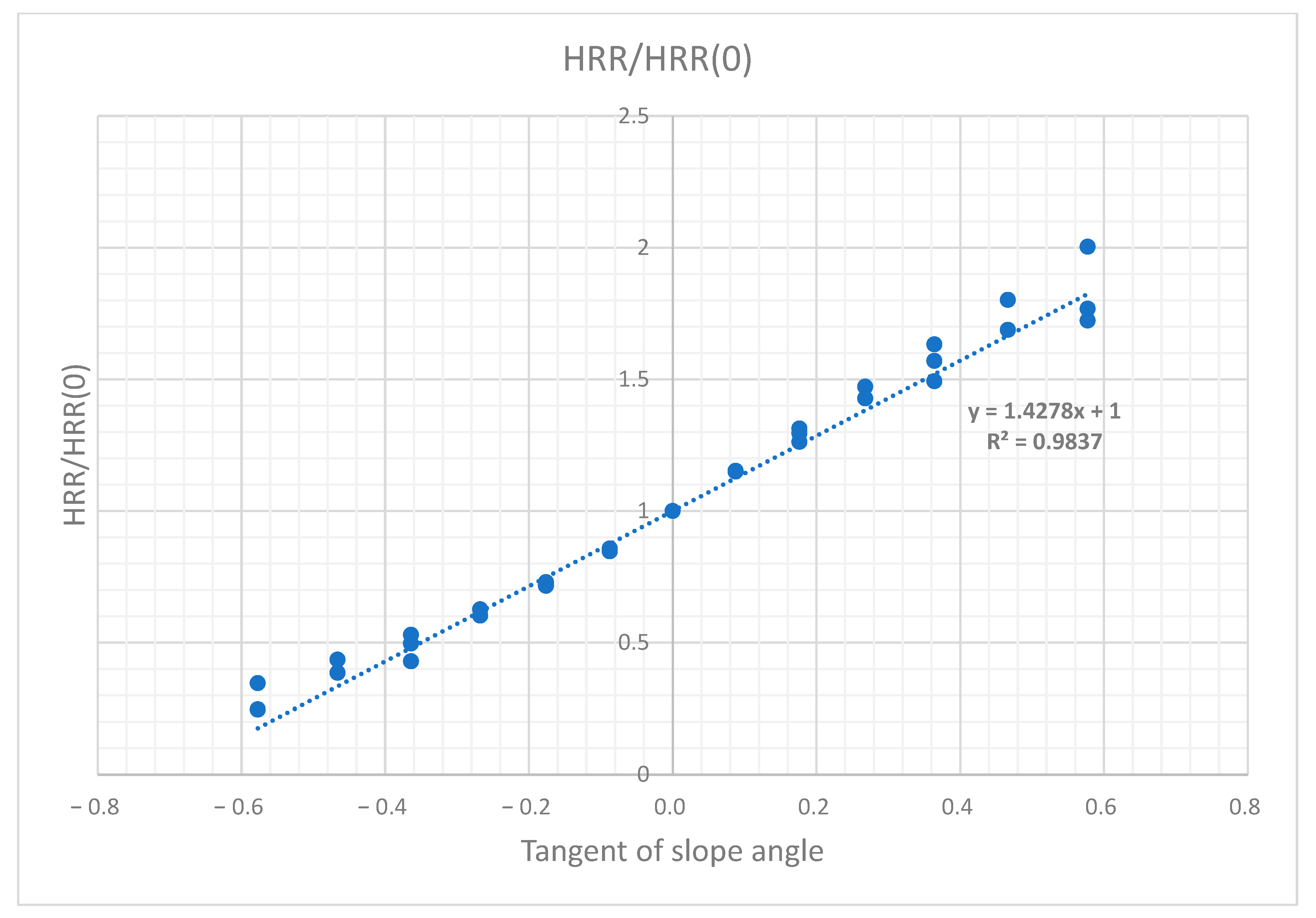
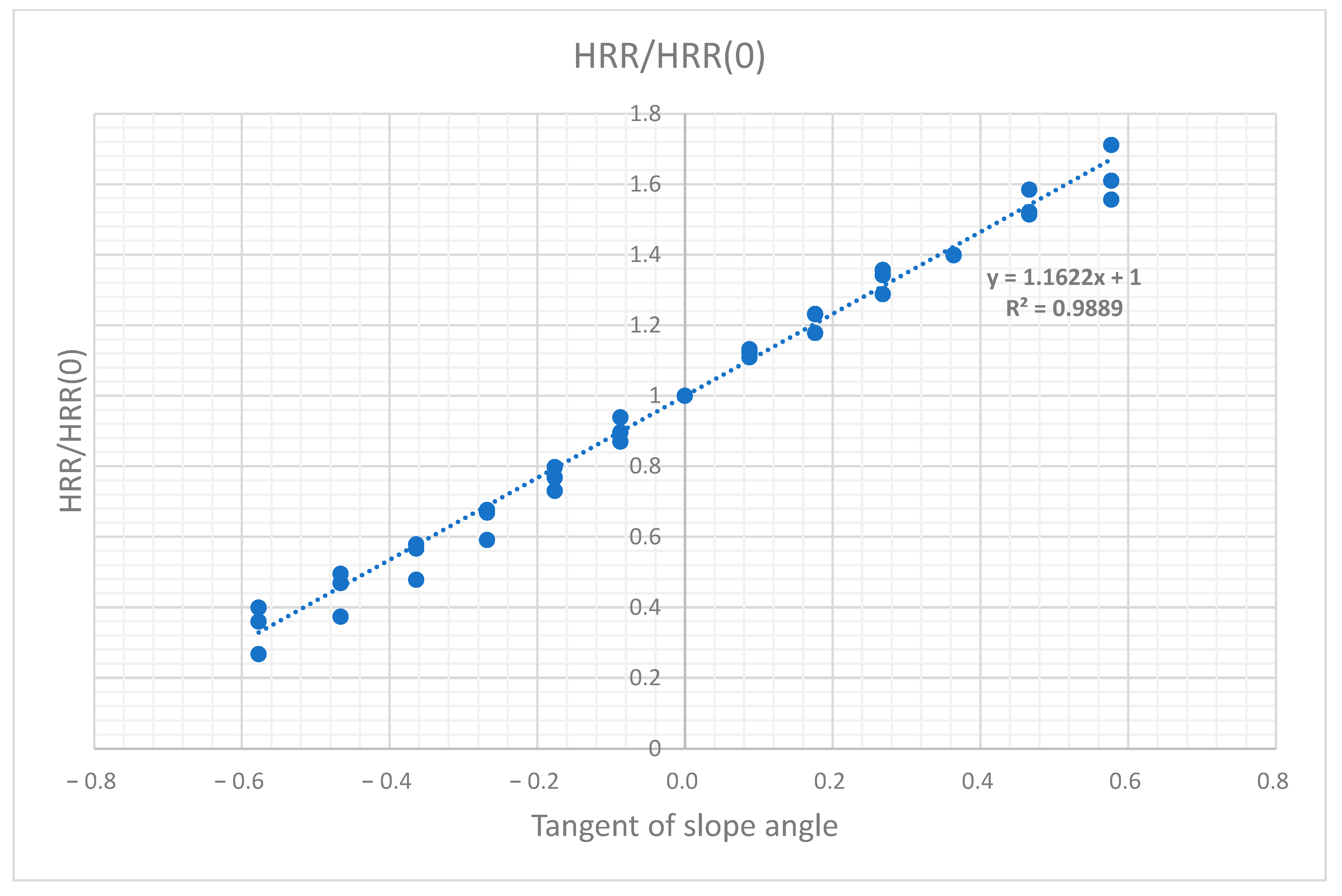
4.4. New Model Proposal

The HRR graphs presented in Figure 9, Figure 10, Figure 11, Figure 16, Figure 17 and Figure 18 demonstrate a steady-state regime following the initial ignition phase. To quantify the influence of slope on fire spread, the average HRR values for each slope and wind velocity, across different tree heights, are summarized in the figures below. The ordinate axes of the graphs represent the HRR/HRR(0) metric, which denotes the ratio of the HRR relative to the zero-slope reference case for a given wind speed and slope. This metric has been selected as a key parameter for this analysis due to its relevance in characterizing fire behavior. However, numerous studies, such as [10], primarily focus on the ROS measured in m/s.

As illustrated in Figure 19 for the 2 m case, the curves corresponding to different wind speeds are closely aligned, demonstrating a near-linear relationship with respect to changes in slope. This suggests that wind speed has a minimal effect on the HRR/HRR(0°) metric. Therefore, the slope of the linear curve can be considered a reliable approximation of the slope effect on fire behavior, with wind speed having a negligible influence on this particular metric.

Figure 20 presents the relationship between the tangent of the slope angle (tan θ) and the normalized heat release rate (HRR/HRR(0)) for a 2 m tree height plantation. The tangent of the slope angle is used to quantitatively represent the steepness of the terrain and to assess its influence on HRR. By using tan(θ), the slope effect can be analyzed in a continuous and mathematically tractable form. Data for various wind speeds are displayed together on a single graph. The correlation coefficient exceeds 0.98, indicating a very strong linear relationship between HRR and the slope angle, as expressed by tan(θ).

Based on the graphs, the following equation can be derived.

$${\displaystyle \frac{HRR}{HRR\left(0\right)}}=1+1.4278\ast \tan \left(slope angle\right)$$

(16)

The slope angle θ is expressed in degrees, and the tangent function is applied after converting θ to radians. HRR/HRR₀ is represented directly as a function of the tangent of the slope angle, following the approach proposed by [10,13], who expressed their relationships in terms of slope percentage. However, in the present study, the correlation coefficient based on the slope angle in degrees is even higher. The proposed formula is applicable to cases with a constant slope and uniform vegetation consisting of 2 m tall trees planted in a regular rectangular pattern, as illustrated in Figure 14.

A similar study was conducted on the 5 m tree cases and the graphs show the results in Figure 21 and Figure 22.

The 5 m tree plantation also shows little to no effect of wind speed on the HRR/HRR(0) metric for different slopes. However, the correlation coefficient between the slope and the HRR is lower, and the formula is as follows.

$${\displaystyle \frac{HRR}{HRR\left(0\right)}}=1+1.1622\ast \tan \left(slope angle\right)$$

(17)

As a main observation, it is worth noting that the computations performed in this study do not demonstrate a clear exponential increase in HRR, but rather a linear growth with the slope angle or its tangent. However, the reason of the coefficient 1.1622 for the 5 m tree plantation and 1.4278 for the 2 m tree plantation remains unclear, and is worth investigating further by running more simulations with different tree sizes. Another idea consists of varying several other parameters such as the tree planting patterns by changing the type of the 2D planting Bravais lattice with a hexagonal pattern or the distance between the trees.

5. Conclusions

This study utilized FDS simulations to investigate wildfire propagation in Douglas Fir tree plantations under varying slopes and wind conditions. Through a structured four-phase approach, we gained valuable insights into fire behavior dynamics that can inform and improve wildfire management strategies.

Phase one validated our numerical model against experimental data from Mell et al. [9] for a single 5 m Douglas Fir tree. The grid sensitivity analysis established that a 50 mm mesh provided optimal balance between computational efficiency and accuracy, with simulated HRR and MLR closely matching experimental data.

The second phase expanded to 66 trees (2 m height), and was validated against Moinuddin and Sutherland [19]. A 200 mm grid size was identified as optimal for plantation-scale simulations. Examining slopes (−30° to +30°) and wind speeds (3 m/s, 6 m/s, 12 m/s) revealed that negative slopes produced lower peak HRR but extended combustion duration, while positive slopes generated higher peak HRR with shorter burnout times. Wind speeds of 12 m/s increased HRR amplitude by approximately 30% compared to 6 m/s.

The third phase extended the model to 5 m tree plantations, confirming similar fundamental fire behavior while revealing variations in HRR intensity. The grid independence analysis validated the 200 mm mesh resolution as sufficient for capturing essential fire dynamics.

Finally, we developed a mathematical model quantifying the relationship between slope angle and HRR. By analyzing the normalized ratio HRR/HRR(0), we identified a strong linear correlation with slope tangent for both tree heights.

For 2 m trees:

HRR/HRR (0) = 1 + 1.4278 × tan (slope angle)

For 5 m trees:

HRR/HRR (0) = 1 + 1.1622 × tan (slope angle)

Notably, wind speed showed minimal effect on this normalized metric, while tree height significantly influenced the slope coefficient. This relationship is attributed to enhanced fuel preheating and increased convective heat transfer on steeper slopes.

This research demonstrates the capability of physics-based CFD to model wildfire dynamics in complex terrains. The findings contribute to an improved understanding of fire behavior in varying landscapes, with practical applications for fire management and risk mitigation. Future work should extend these simulations to broader topographic variations and diverse vegetation arrangements, including heterogeneous tree sizes, mixed species, and non-uniform spacing patterns that better represent natural forest conditions, to further refine predictive models for wildfire spread in real-world environments.

References

1. Morandini, F.; Silvani, X. Experimental investigation of the physical mechanisms governing the spread of wildfires. Int. J. Wildland Fire 2010, 19, 570–582. [Google Scholar] [CrossRef]
2. Silvani, X.; Morandini, F.; Muzy, J.-F. Wildfire spread experiments: Fluctuations in thermal measurements. Int. Commun. Heat Mass Transf. 2009, 36, 887–892. [Google Scholar] [CrossRef]
3. Mueller, E.V.; Skowronski, N.; Thomas, J.C.; Clark, K.; Gallagher, M.R.; Hadden, R.; Mell, W.; Simeoni, A. Local measurements of wildland fire dynamics in a field-scale experiment. Combust. Flame 2018, 194, 452–463. [Google Scholar] [CrossRef]
4. Balbi, J.H.; Morandini, F.; Silvani, X.; Filippi, J.B.; Rinieri, F. A physical model for wildland fires. Combust. Flame 2009, 156, 2217–2230. [Google Scholar] [CrossRef]
5. Mell, W.; Jenkins, M.A.; Gould, J.; Cheney, P. A physics-based approach to modelling grassland fires. Int. J. Wildland Fire 2007, 16, 1–22. [Google Scholar] [CrossRef]
6. Morvan, D.; Meradji, S.; Accary, G. Physical modelling of fire spread in grasslands. Fire Saf. J. 2009, 44, 50–61. [Google Scholar] [CrossRef]
7. Dupuy, J.-L.; Morvan, D. Numerical study of a crown fire spreading toward a fuel break using a multiphase physical model. Int. J. Wildland Fire 2005, 14, 141–151. [Google Scholar] [CrossRef]
8. Linn, R.; Winterkamp, J.; Edminster, C.; Colman, J.J.; Smith, W.S. Coupled influences of topography and wind on wildland fire behaviour. Int. J. Wildland Fire 2007, 16, 183–195. [Google Scholar] [CrossRef]
9. Mell, W.; Maranghides, A.; McDermott, R.; Manzello, S.L. Numerical simulation and experiments of burning douglas fir trees. Combust. Flame 2009, 156, 2023–2041. [Google Scholar] [CrossRef]
10. Goetz, G.O. A Statistical Investigation of How Slope Affects a Wildfire’s Rate of Spread. Master’s Thesis, University of British Columbia, Vancouver, BC, Canada, 2021. [Google Scholar]
11. Sharples, J.J. Review of formal methodologies for wind–slope correction of wildfire rate of spread. Int. J. Wildland Fire 2008, 17, 179–193. [Google Scholar] [CrossRef]
12. McArthur, A.G. Weather and Grassland Fire Behaviour; Forestry Timber Bureau Australia: Camperdown, NSW, Australia, 1966. [Google Scholar]
13. McAlpine, R.S.L.; Bruce, D.; Taylor, E. Fire spread across a slope. In Proceedings of the 11th Conference on Fire and Forest Meteorology, Missoula, MT, USA, 16–19 April 1991; Society of American Foresters: Bethesda, MD, USA, 1991; pp. 218–255. [Google Scholar]
14. Pagni, P.J.; Peterson, T.G. Flame spread through porous fuels. Symp. (Int.) Combust. 1973, 14, 1099–1107. [Google Scholar] [CrossRef]
15. Valero Pérez, M.M.; Pastor Ferrer, E.; Mata, C.; Rios Rubiras, O.; Planas Cuchi, E.; Parsons, R. Computing wildfire behaviour metrics from CFD simulation data. In Proceedings of the 6th International Fire Behavior and Fuels Conference, Marseilles, France, 29 April–3 May 2019; pp. 1–6. [Google Scholar]
16. Pimont, F.; Dupuy, J.-L.; Linn, R.R. Coupled slope and wind effects on fire spread with influences of fire size: A numerical study using FIRETEC. Int. J. Wildland Fire 2012, 21, 828–842. [Google Scholar] [CrossRef]
17. Linn, R.R.; Winterkamp, J.L.; Weise, D.R.; Edminster, C. A numerical study of slope and fuel structure effects on coupled wildfire behaviour. Int. J. Wildland Fire 2010, 19, 179–201. [Google Scholar] [CrossRef]
18. Simpson, C.C.; Sharples, J.J.; Evans, J.P.; McCabe, M.F. Large eddy simulation of atypical wildland fire spread on leeward slopes. Int. J. Wildland Fire 2013, 22, 599–614. [Google Scholar] [CrossRef]
19. Moinuddin, K.A.; Sutherland, D. Modelling of tree fires and fires transitioning from the forest floor to the canopy with a physics-based model. Math. Comput. Simul. 2020, 175, 81–95. [Google Scholar] [CrossRef]
20. Kim, D.-W.; Chung, W.; Lee, B. Exploring tree crown spacing and slope interaction effects on fire behavior with a physics-based fire model. For. Sci. Technol. 2016, 12, 167–175. [Google Scholar] [CrossRef]
21. Miloua, H. Numerical prediction of the fire spread in vegetative fuels using NISTWFDS Model. Int. J. Eng. Res. Afr. 2016, 20, 177–192. [Google Scholar] [CrossRef]
22. McGrattan, K.; Hostikka, S.; Floyd, J.; Baum, H.; Rehm, R.; Mell, W.; McDermott, R. Fire Dynamics Simulator (Version 5) Technical Reference Guide; NIST Special Publication 1018-5; National Institute of Standards and Technology: Gaithersburg, MD, USA, 2010.
23. McGrattan, K.; Hostikka, S.; McDermott, R.; Floyd, J.; Weinschenk, C.; Overholt, K. Fire Dynamics Simulator User’s Guide; NIST Special Publication 1019; National Institute of Standards and Technology: Gaithersburg, MD, USA, 2013; pp. 1–339.
24. Hayajneh, S.M. Numerical Simulation of Fire Spread in Multi-Story Cross Laminated Timber Buildings. Master’s Thesis, Swinburne University of Technology, Melbourne, Australia, 2022. [Google Scholar]
25. Hayajneh, S.M.; Naser, J. Fire Spread in Multi-Storey Timber Building, a CFD Study. Fluids 2023, 8, 140. [Google Scholar] [CrossRef]
26. Morvan, D.; Dupuy, J.-L. Modeling the propagation of a wildfire through a Mediterranean shrub using a multiphase formulation. Combust. Flame 2004, 138, 199–210. [Google Scholar] [CrossRef]
27. Morvan, D.; Meradji, S.; Mell, W. Interaction between head fire and backfire in grasslands. Fire Saf. J. 2013, 58, 195–203. [Google Scholar] [CrossRef]
28. Moinuddin, K.; Sutherland, D.; Mell, W. Simulation study of grass fire using a physics-based model: Striving towards numerical rigour and the effect of grass height on the rate of spread. Int. J. Wildland Fire 2018, 27, 800–814. [Google Scholar] [CrossRef]
29. Nelson Jr, R.M. An effective wind speed for models of fire spread. Int. J. Wildland Fire 2002, 11, 153–161. [Google Scholar] [CrossRef]
Figure 1. Douglas Fir tree shape and terminology.
Fire 08 00217 g001
Figure 2. Model representation at zero slope.
Fire 08 00217 g002
Figure 3. (a) Fire simulation model for 5 m single fir tree with computational domain dimensions (6.4 × 3.2 × 12.8 m), (b,c) simulations of 5 m single Douglas Fir tree at various time points after ignition corresponding to the temperature contours shown in Figure 4.
Fire 08 00217 g003
Figure 4. Gas-phase temperature contours for simulations of a 5 m single Douglas Fir tree at various time points after ignition.
Fire 08 00217 g004
Figure 5. Comparison of the MLS for simulating a 5 m single Douglas Fir tree with experiment [9] for 100 mm, 50 mm, and 37.5 mm grid sizes using FDS.
Fire 08 00217 g005
Figure 6. Comparison of the HRR for simulating a 5 m single Douglas Fir tree for grid sizes of 100 mm, 50 mm, and 37.5 mm using FDS.
Fire 08 00217 g006
Figure 7. Visual representation of the different slope configurations used in this study. The figure illustrates how various terrain inclinations were modeled to analyze the impact of slope on fire spread behavior.
Fire 08 00217 g007
Figure 8. Comparison of the simulation of 66 trees by Moinuddin and Sutherland (2020) [19], with the current model at 100, 200, and 400 mm grid sizes, using the same velocity and parameters, to validate the current model.
Fire 08 00217 g008
Figure 9. Model comparison of simulation results for 66 Douglas Fir trees (2 m height) at a 200 mm grid size and 3 m/s wind velocity with different slopes.
Fire 08 00217 g009
Figure 10. Model comparison of simulation results for 66 Douglas Fir trees (2 m height) at a 200 mm grid size and 6 m/s wind velocity with different slopes.
Fire 08 00217 g010
Figure 11. Model comparison of simulation results for 66 Douglas Fir trees (2 m height) at a 200 mm grid size and 12 m/s wind velocity with different slopes.
Fire 08 00217 g011
Figure 12. Overview of the primary dimensions of the computational domain for a plantation featuring 5 m tall trees, including the flame dynamics upon impacting the tree crowns.
Fire 08 00217 g012
Figure 13. Snapshot capturing the burning plantation at t = 180 s, showing quasi-steady flame propagation as the HRR fluctuates near its maximum value.
Fire 08 00217 g013
Figure 14. Top view of the 3D domain.
Fire 08 00217 g014
Figure 15. Comparison of simulation results for 66 Douglas Fir trees (5 m height) at different grid sizes (400 mm, 200 mm, and 100 mm).
Fire 08 00217 g015
Figure 16. Model comparison of simulation results for 66 Douglas Fir trees (5 m height) at a 200 mm grid size and 3 m/s wind velocity with different slopes.
Fire 08 00217 g016
Figure 17. Model comparison of simulation results for 66 Douglas Fir trees (5 m height) at a 200 mm grid size and 6 m/s wind velocity with different slopes.
Fire 08 00217 g017
Figure 18. Model comparison of simulation results for 66 Douglas Fir trees (5 m height) at a 200 mm grid size and 12 m/s wind velocity with different slopes.
Fire 08 00217 g018
Figure 19. Slope effect comparison at different wind speeds for 2 m plantation model.
Fire 08 00217 g019
Figure 20. Slope effect correlation analysis for the 2 m plantation model, showing the relationship between the tangent of the slope angle in degrees (tan θ) and the normalized heat release rate (HRR/HRR(0)).
Fire 08 00217 g020
Figure 21. Slope effect comparison at different wind speeds for 5 m plantation model.
Fire 08 00217 g021
Figure 22. Slope effect correlation analysis for the 5 m plantation model showing the relationship between the tangent of the slope angle in degrees (tan θ) and the normalized heat release rate (HRR/HRR(0)).
Fire 08 00217 g022