Post-Fire Burned Area Detection Using Machine Learning and Burn Severity Classification with Spectral Indices in İzmir: A SHAP-Driven XAI Approach


Abstract
:1. Introduction
- i.
- Integration of ML and Spectral Indices for Burned Area Classification: While the dNBR and dNDVI provide an initial assessment of burn severity, this study demonstrates that ML algorithms—RF, LightGBM, XGBoost, and AdaBoost—offer data-driven alternatives that are capable of capturing complex spectral variations beyond simple threshold-based classifications.
- ii.
- Optimized Model Performance through Hyperparameter Tuning: Unlike conventional approaches, this study applies hyperparameter optimization to improve the predictive accuracy of ML-based burned area detection, which is assessed using multiple evaluation metrics, including the overall accuracy (OA), Kappa coefficient (κ), and F1 score (FS).
- iii.
- Explainable AI (XAI) for Enhanced Interpretability: The integration of SHAP (SHapley Additive exPlanations) within the Explainable AI (XAI) framework allows for a transparent analysis of the most influential spectral and environmental factors in fire severity classification.
- iv.
- Scalable and Data-Driven Approach for Fire Management: By leveraging ML’s predictive capabilities alongside XAI-driven explanations, this study provides a robust, interpretable, and scalable methodology for post-fire ecosystem monitoring. The findings are expected to contribute to more effective fire management policies, post-fire recovery planning, and data-driven decision-making in fire-prone regions like İzmir.
2. Materials and Methods
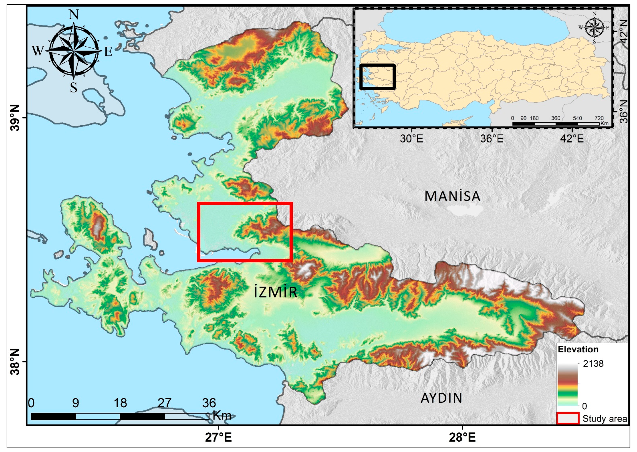
2.1. Study Area
2.2. Dataset
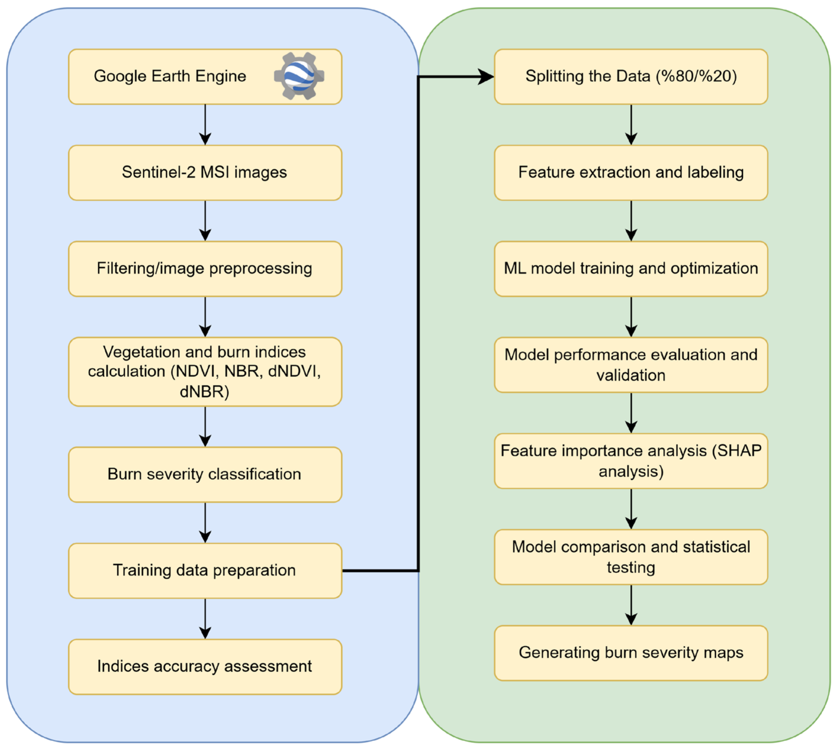
2.3. Methods
2.3.1. Image Preprocessing
2.3.2. Creation of Training and Test Samples
2.3.3. Machine Learning Algorithms
2.3.4. Hyperparameters Tuning
2.3.5. SHapley Additive exPlanations
2.3.6. Accuracy Assessment
3. Results
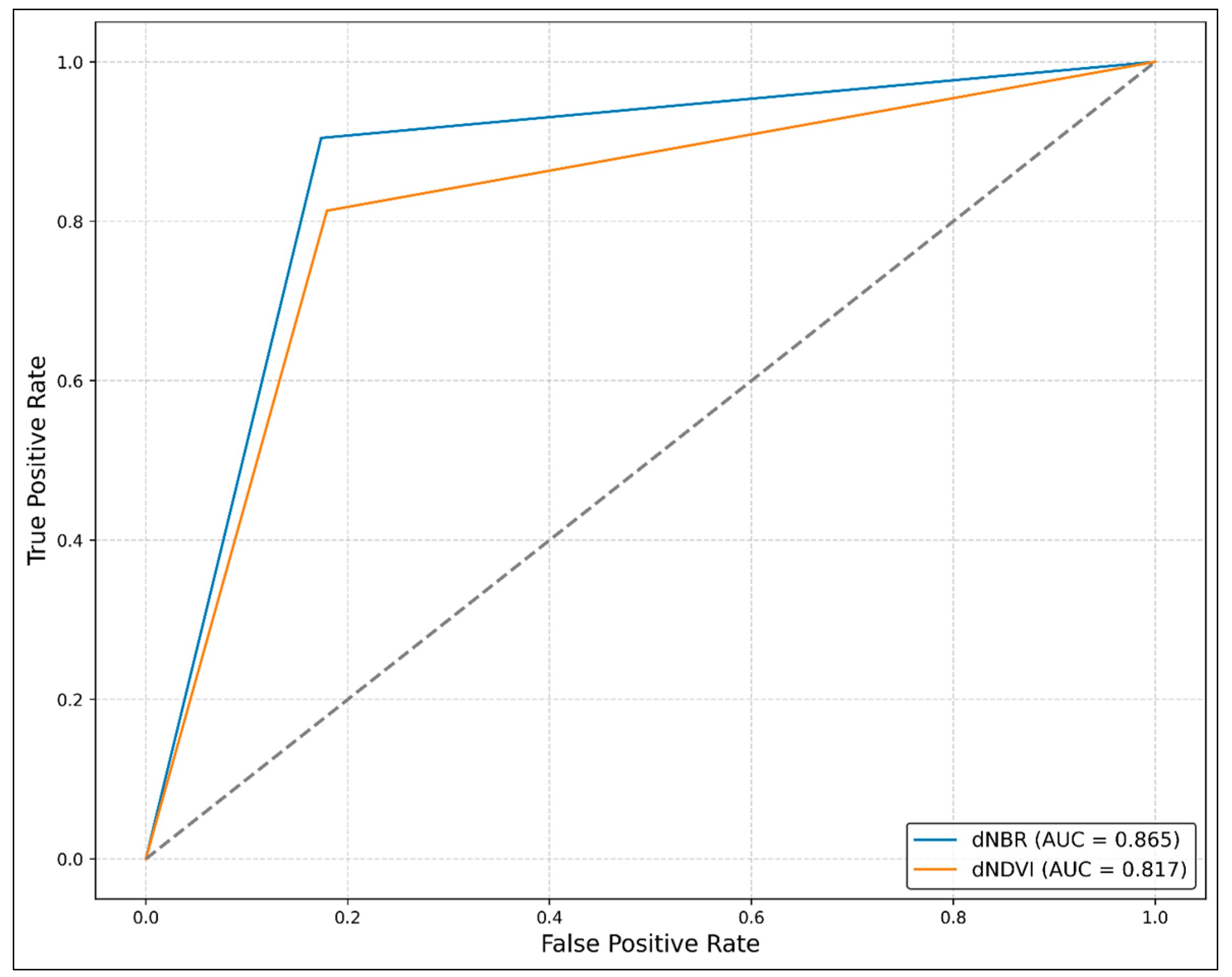
3.1. Index-Based Results
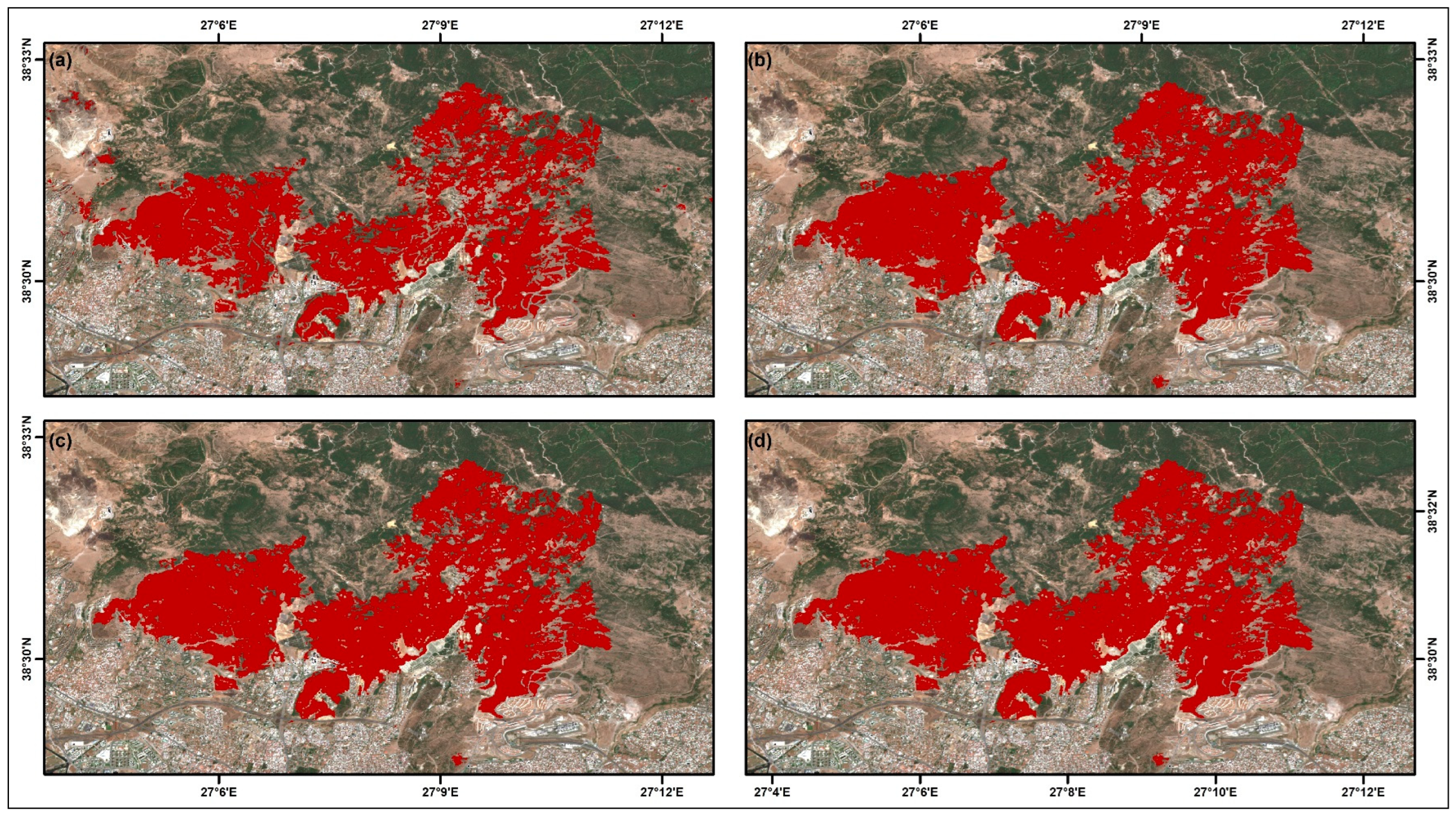
3.2. ML-Based Results
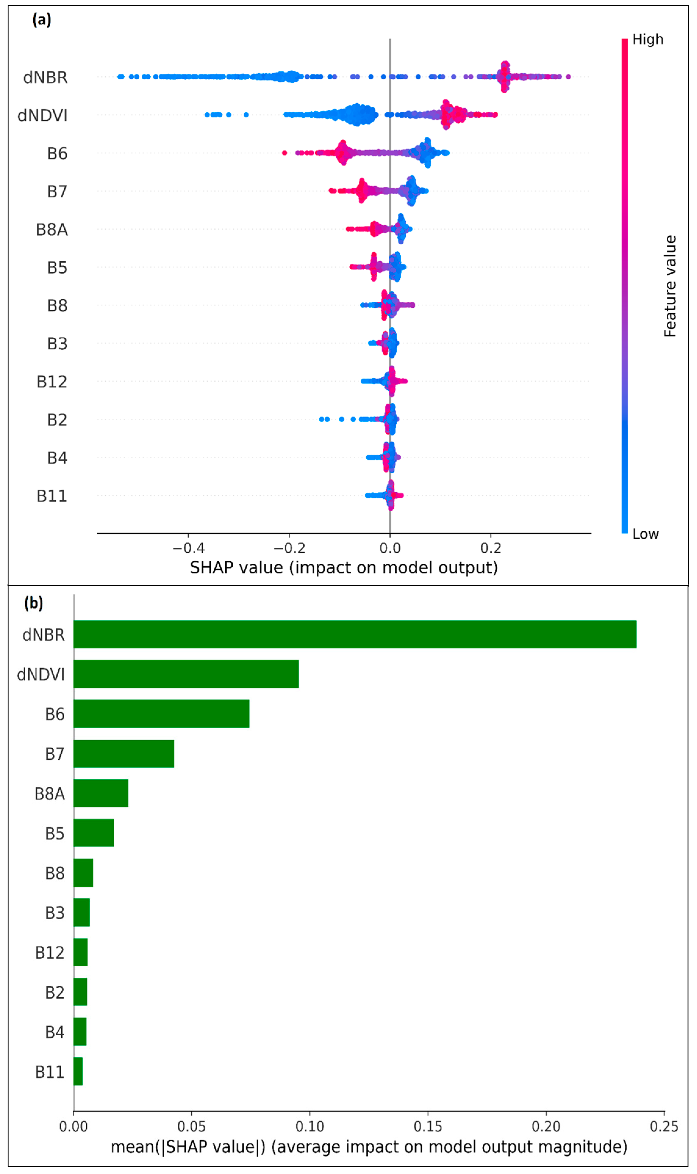
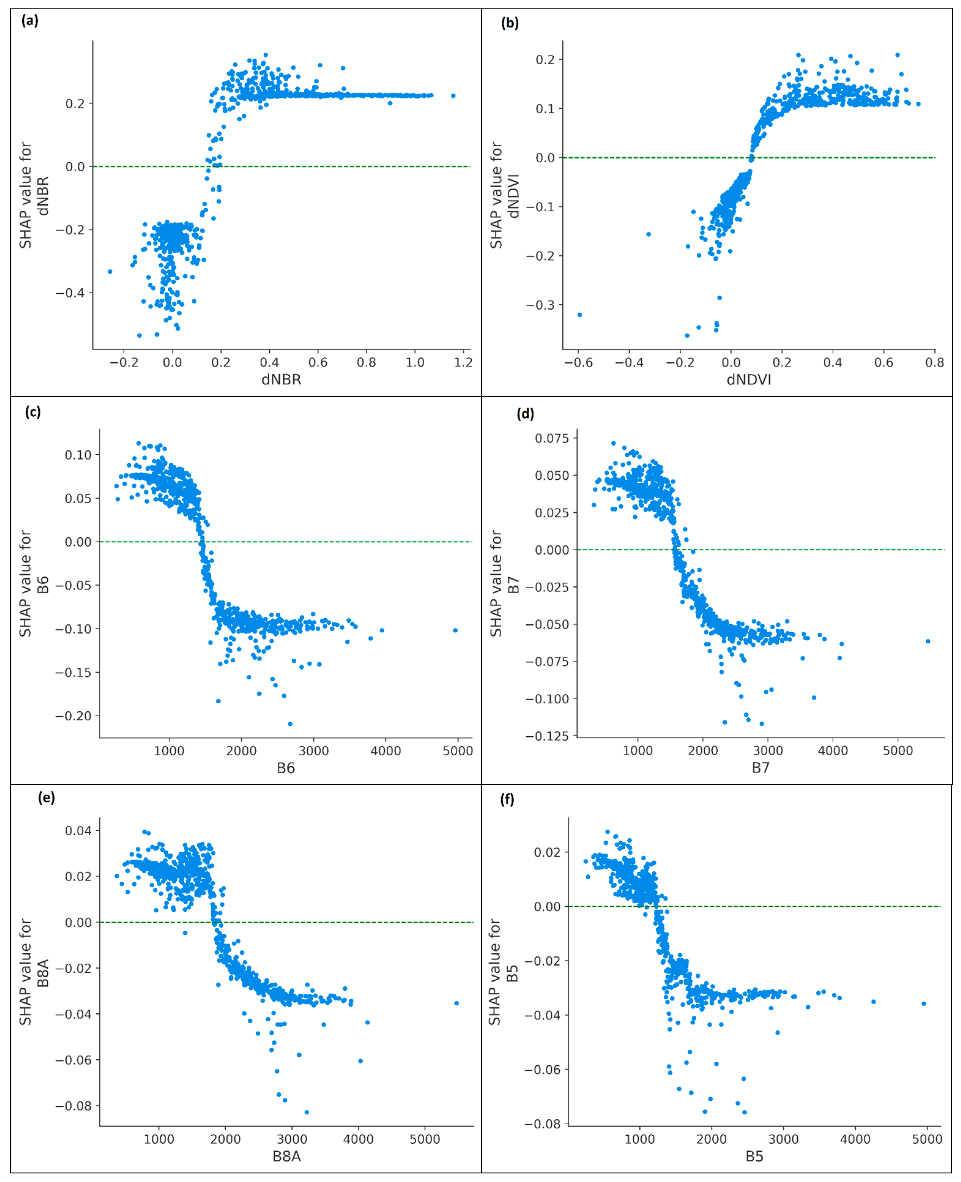
3.3. Analysis of SHAP-Based Feature Importance
4. Discussion
5. Conclusions
Author Contributions
Funding
Institutional Review Board Statement
Informed Consent Statement
Data Availability Statement
Acknowledgments
Conflicts of Interest
References
- Barrios, E.; Valencia, V.; Jonsson, M.; Brauman, A.; Hairiah, K.; Mortimer, P.E.; Okubo, S. Contribution of Trees to the Conservation of Biodiversity and Ecosystem Services in Agricultural Landscapes. Int. J. Biodivers. Sci. Ecosyst. Serv. Manag. 2018, 14, 1–16. [Google Scholar]
- Psistaki, K.; Tsantopoulos, G.; Paschalidou, A.K. An Overview of the Role of Forests in Climate Change Mitigation. Sustainability 2024, 16, 6089. [Google Scholar] [CrossRef]
- Thompson, I.; Mackey, B.; McNulty, S.; Mosseler, A. Forest Resilience, Biodiversity, and Climate Change: A Synthesis of the Biodiversity/Resiliende/Stability Relationship in Forest Ecosystems; Thompson, I.D., Ed.; CBD technical series; Secretariat of the Convention on Biological Diversity: Montreal, QC, Canada, 2009; ISBN 978-92-9225-137-6.
- Gago, E.J.; Roldan, J.; Pacheco-Torres, R.; Ordóñez, J. The City and Urban Heat Islands: A Review of Strategies to Mitigate Adverse Effects. Renew. Sustain. Energy Rev. 2013, 25, 749–758. [Google Scholar] [CrossRef]
- Hisano, M.; Searle, E.B.; Chen, H.Y.H. Biodiversity as a Solution to Mitigate Climate Change Impacts on the Functioning of Forest Ecosystems. Biol. Rev. Camb. Philos. Soc. 2018, 93, 439–456. [Google Scholar] [CrossRef]
- Kinoshita, A.M.; Chin, A.; Simon, G.L.; Briles, C.; Hogue, T.S.; O’Dowd, A.P.; Gerlak, A.K.; Albornoz, A.U. Wildfire, Water, and Society: Toward Integrative Research in the “Anthropocene”. Anthropocene 2016, 16, 16–27. [Google Scholar] [CrossRef]
- Bowman, D.M.J.S.; Williamson, G.J.; Gibson, R.K.; Bradstock, R.A.; Keenan, R.J. The Severity and Extent of the Australia 2019–20 Eucalyptus Forest Fires Are Not the Legacy of Forest Management. Nat. Ecol. Evol. 2021, 5, 1003–1010. [Google Scholar] [CrossRef]
- dos Reis, M.; de Alencastro Graça, P.M.L.; Yanai, A.M.; Ramos, C.J.P.; Fearnside, P.M. Forest Fires and Deforestation in the Central Amazon: Effects of Landscape and Climate on Spatial and Temporal Dynamics. J. Environ. Manag. 2021, 288, 112310. [Google Scholar] [CrossRef]
- Cova, G.; Kane, V.R.; Prichard, S.; North, M.; Cansler, C.A. The Outsized Role of California’s Largest Wildfires in Changing Forest Burn Patterns and Coarsening Ecosystem Scale. For. Ecol. Manag. 2023, 528, 120620. [Google Scholar] [CrossRef]
- Fernández-Guisuraga, J.M.; Suárez-Seoane, S.; García-Llamas, P.; Calvo, L. Vegetation Structure Parameters Determine High Burn Severity Likelihood in Different Ecosystem Types: A Case Study in a Burned Mediterranean Landscape. J. Environ. Manag. 2021, 288, 112462. [Google Scholar] [CrossRef]
- Balde, B.; Vega-Garcia, C.; Gelabert, P.J.; Ameztegui, A.; Rodrigues, M. The Relationship between Fire Severity and Burning Efficiency for Estimating Wildfire Emissions in Mediterranean Forests. J. For. Res. 2023, 34, 1195–1206. [Google Scholar] [CrossRef]
- Dosiou, A.; Athinelis, I.; Katris, E.; Vassalou, M.; Kyrkos, A.; Krassakis, P.; Parcharidis, I. Employing Copernicus Land Service and Sentinel-2 Satellite Mission Data to Assess the Spatial Dynamics and Distribution of the Extreme Forest Fires of 2023 in Greece. Fire 2024, 7, 20. [Google Scholar] [CrossRef]
- Artés, T.; Oom, D.; de Rigo, D.; Durrant, T.H.; Maianti, P.; Libertà, G.; San-Miguel-Ayanz, J. A Global Wildfire Dataset for the Analysis of Fire Regimes and Fire Behaviour. Sci. Data 2019, 6, 296. [Google Scholar] [CrossRef]
- Yue, C.; Ciais, P.; Cadule, P.; Thonicke, K.; van Leeuwen, T.T. Modelling the Role of Fires in the Terrestrial Carbon Balance by Incorporating SPITFIRE into the Global Vegetation Model ORCHIDEE—Part 2: Carbon Emissions and the Role of Fires in the Global Carbon Balance. Geosci. Model Dev. 2015, 8, 1321–1338. [Google Scholar] [CrossRef]
- Rozario, P.F.; Madurapperuma, B.D.; Wang, Y. Remote Sensing Approach to Detect Burn Severity Risk Zones in Palo Verde National Park, Costa Rica. Remote Sens. 2018, 10, 1427. [Google Scholar] [CrossRef]
- Tepley, A.J.; Thomann, E.; Veblen, T.T.; Perry, G.L.W.; Holz, A.; Paritsis, J.; Kitzberger, T.; Anderson-Teixeira, K.J. Influences of Fire–Vegetation Feedbacks and Post-Fire Recovery Rates on Forest Landscape Vulnerability to Altered Fire Regimes. J. Ecol. 2018, 106, 1925–1940. [Google Scholar] [CrossRef]
- General Directory of Forestry. Forest Fire Fighting Activities 2023 Evaluation Report; General Directory of Forestry: Ankara, Turkey, 2023. Available online: https://www.ogm.gov.tr (accessed on 23 December 2024).
- Güngöroğlu, C.; Özkara, Z.U.; Tutmaz, V. Türkiye’de Orman Yangın Yönetimi: Sorunlar ve Çözüm Önerileri. Memleket. Siyaset. Önetim. 2024, 19, 517–570. [Google Scholar] [CrossRef]
- Izmir Governorship Provincial Disaster and Emergency Directorate. Izmir Provincial Disaster Risk Reduction Plan; Izmir Governorship Provincial Disaster and Emergency Directorate: Istanbul, Turkey, 2024; 326p. [Google Scholar]
- Cardil, A.; Mola-Yudego, B.; Blázquez-Casado, Á.; González-Olabarria, J.R. Fire and Burn Severity Assessment: Calibration of Relative Differenced Normalized Burn Ratio (RdNBR) with Field Data. J. Environ. Manag. 2019, 235, 342–349. [Google Scholar] [CrossRef]
- Boroujeni, S.P.H.; Razi, A.; Khoshdel, S.; Afghah, F.; Coen, J.L.; O’Neill, L.; Fule, P.; Watts, A.; Kokolakis, N.-M.T.; Vamvoudakis, K.G. A Comprehensive Survey of Research towards AI-Enabled Unmanned Aerial Systems in Pre-, Active-, and Post-Wildfire Management. Inf. Fusion 2024, 108, 102369. [Google Scholar] [CrossRef]
- Dixon, D.J.; Callow, J.N.; Duncan, J.M.A.; Setterfield, S.A.; Pauli, N. Regional-Scale Fire Severity Mapping of Eucalyptus Forests with the Landsat Archive. Remote Sens. Environ. 2022, 270, 112863. [Google Scholar] [CrossRef]
- Chuvieco, E.; Aguado, I.; Salas, J.; García, M.; Yebra, M.; Oliva, P. Satellite Remote Sensing Contributions to Wildland Fire Science and Management. Curr. For. Rep. 2020, 6, 81–96. [Google Scholar] [CrossRef]
- Kurbanov, E.; Vorobev, O.; Lezhnin, S.; Sha, J.; Wang, J.; Li, X.; Cole, J.; Dergunov, D.; Wang, Y. Remote Sensing of Forest Burnt Area, Burn Severity, and Post-Fire Recovery: A Review. Remote Sens. 2022, 14, 4714. [Google Scholar] [CrossRef]
- Lanorte, A.; Danese, M.; Lasaponara, R.; Murgante, B. Multiscale Mapping of Burn Area and Severity Using Multisensor Satellite Data and Spatial Autocorrelation Analysis. Int. J. Appl. Earth Obs. Geoinf. 2013, 20, 42–51. [Google Scholar] [CrossRef]
- İban, M.C.; Şahin, E. Monitoring Burn Severity and Air Pollutants in Wildfire Events Using Remote Sensing Data: The Case of Mersin Wildfires in Summer 2021. Gümüşhane Üniversitesi Fen Bilim. Derg. 2022, 12, 487–497. [Google Scholar] [CrossRef]
- Urbanski, S.P.; Salmon, J.M.; Nordgren, B.L.; Hao, W.M. A MODIS Direct Broadcast Algorithm for Mapping Wildfire Burned Area in the Western United States. Remote Sens. Environ. 2009, 113, 2511–2526. [Google Scholar] [CrossRef]
- Libonati, R.; DaCamara, C.C.; Pereira, J.M.C.; Peres, L.F. Retrieving Middle-Infrared Reflectance for Burned Area Mapping in Tropical Environments Using MODIS. Remote Sens. Environ. 2010, 114, 831–843. [Google Scholar] [CrossRef]
- Krylov, A.; McCarty, J.L.; Potapov, P.; Loboda, T.; Tyukavina, A.; Turubanova, S.; Hansen, M.C. Remote Sensing Estimates of Stand-Replacement Fires in Russia, 2002–2011. Environ. Res. Lett. 2014, 9, 105007. [Google Scholar] [CrossRef]
- Chu, T.; Guo, X.; Takeda, K. Remote Sensing Approach to Detect Post-Fire Vegetation Regrowth in Siberian Boreal Larch Forest. Ecol. Indic. 2016, 62, 32–46. [Google Scholar] [CrossRef]
- Howe, A.A.; Parks, S.A.; Harvey, B.J.; Saberi, S.J.; Lutz, J.A.; Yocom, L.L. Comparing Sentinel-2 and Landsat 8 for Burn Severity Mapping in Western North America. Remote Sens. 2022, 14, 5249. [Google Scholar] [CrossRef]
- Henry, M.C.; Maingi, J.K. Evaluating Landsat- and Sentinel-2-Derived Burn Indices to Map Burn Scars in Chyulu Hills, Kenya. Fire 2024, 7, 472. [Google Scholar] [CrossRef]
- Mallinis, G.; Mitsopoulos, I.; Chrysafi, I. Evaluating and Comparing Sentinel 2A and Landsat-8 Operational Land Imager (OLI) Spectral Indices for Estimating Fire Severity in a Mediterranean Pine Ecosystem of Greece. GIScience Remote Sens. 2018, 55, 1–18. [Google Scholar] [CrossRef]
- Bar, S.; Parida, B.R.; Pandey, A.C. Landsat-8 and Sentinel-2 Based Forest Fire Burn Area Mapping Using Machine Learning Algorithms on GEE Cloud Platform over Uttarakhand, Western Himalaya. Remote Sens. Appl. Soc. Environ. 2020, 18, 100324. [Google Scholar] [CrossRef]
- Mashhadi, N.; Alganci, U. Determination of Forest Burn Scar and Burn Severity from Free Satellite Images: A Comparative Evaluation of Spectral Indices and Machine Learning Classifiers. Int. J. Environ. Geoinform. 2021, 8, 488–497. [Google Scholar] [CrossRef]
- Boer, M.M.; Macfarlane, C.; Norris, J.; Sadler, R.J.; Wallace, J.; Grierson, P.F. Mapping Burned Areas and Burn Severity Patterns in SW Australian Eucalypt Forest Using Remotely-Sensed Changes in Leaf Area Index. Remote Sens. Environ. 2008, 112, 4358–4369. [Google Scholar] [CrossRef]
- Robichaud, P.R.; Lewis, S.A.; Laes, D.Y.M.; Hudak, A.T.; Kokaly, R.F.; Zamudio, J.A. Postfire Soil Burn Severity Mapping with Hyperspectral Image Unmixing. Remote Sens. Environ. 2007, 108, 467–480. [Google Scholar] [CrossRef]
- Chen, D.; Fu, C.; Hall, J.V.; Hoy, E.E.; Loboda, T.V. Spatio-Temporal Patterns of Optimal Landsat Data for Burn Severity Index Calculations: Implications for High Northern Latitudes Wildfire Research. Remote Sens. Environ. 2021, 258, 112393. [Google Scholar] [CrossRef]
- Morante-Carballo, F.; Bravo-Montero, L.; Carrión-Mero, P.; Velastegui-Montoya, A.; Berrezueta, E. Forest Fire Assessment Using Remote Sensing to Support the Development of an Action Plan Proposal in Ecuador. Remote Sens. 2022, 14, 1783. [Google Scholar] [CrossRef]
- Gupta, P.; Shukla, A.K.; Shukla, D.P. Sentinel 2 Based Burn Severity Mapping and Assessing Post-Fire Impacts on Forests and Buildings in the Mizoram, a North-Eastern Himalayan Region. Remote Sens. Appl. Soc. Environ. 2024, 36, 101279. [Google Scholar] [CrossRef]
- Tiengo, R.; Merino-De-Miguel, S.; Uchôa, J.; Guiomar, N.; Gil, A. Burned Areas Mapping Using Sentinel-2 Data and a Rao’s Q Index-Based Change Detection Approach: A Case Study in Three Mediterranean Islands’ Wildfires (2019–2022). Remote Sens. 2025, 17, 830. [Google Scholar] [CrossRef]
- Gitelson, A.A. Remote Estimation of Crop Fractional Vegetation Cover: The Use of Noise Equivalent as an Indicator of Performance of Vegetation Indices. Int. J. Remote Sens. 2013, 34, 6054–6066. [Google Scholar] [CrossRef]
- Miller, J.D.; Thode, A.E. Quantifying Burn Severity in a Heterogeneous Landscape with a Relative Version of the Delta Normalized Burn Ratio (dNBR). Remote Sens. Environ. 2007, 109, 66–80. [Google Scholar] [CrossRef]
- Yilmaz, O.S.; Acar, U.; Sanli, F.B.; Gulgen, F.; Ates, A.M. Mapping Burn Severity and Monitoring CO Content in Türkiye’s 2021 Wildfires, Using Sentinel-2 and Sentinel-5P Satellite Data on the GEE Platform. Earth Sci. Inform. 2023, 16, 221–240. [Google Scholar] [CrossRef] [PubMed]
- Key, C.H.; Benson, N.C. Landscape assessment (LA). In FIREMON: Fire Effects Monitoring and Inventory System; Gen. Tech. Rep. RMRS-GTR-164-CD; US Department of Agriculture, Forest Service, Rocky Mountain Research Station: Fort Collins, CO, USA, 2006; p. LA-1-55. [Google Scholar]
- Boucher, J.; Beaudoin, A.; Hébert, C.; Guindon, L.; Bauce, É. Assessing the Potential of the Differenced Normalized Burn Ratio (dNBR) for Estimating Burn Severity in Eastern Canadian Boreal Forests. Int. J. Wildland Fire 2017, 26, 32. [Google Scholar] [CrossRef]
- Chen, D.; Loboda, T.V.; Hall, J.V. A Systematic Evaluation of Influence of Image Selection Process on Remote Sensing-Based Burn Severity Indices in North American Boreal Forest and Tundra Ecosystems. ISPRS J. Photogramm. Remote Sens. 2020, 159, 63–77. [Google Scholar] [CrossRef]
- Lutes, D.C.; Keane, R.E.; Caratti, J.F.; Key, C.H.; Benson, N.C.; Sutherland, S.; Gangi, L.J. FIREMON: Fire Effects Monitoring and Inventory System; U.S. Department of Agriculture, Forest Service, Rocky Mountain Research Station: Fort Collins, CO, USA, 2006; p. RMRS-GTR-164. [Google Scholar]
- Mathews, L.E.H.; Kinoshita, A.M. Urban Fire Severity and Vegetation Dynamics in Southern California. Remote Sens. 2020, 13, 19. [Google Scholar] [CrossRef]
- French, N.H.F.; Kasischke, E.S.; Hall, R.J.; Murphy, K.A.; Verbyla, D.L.; Hoy, E.E.; Allen, J.L. Using Landsat Data to Assess Fire and Burn Severity in the North American Boreal Forest Region: An Overview and Summary of Results. Int. J. Wildland Fire 2008, 17, 443. [Google Scholar] [CrossRef]
- Veraverbeke, S.; Verstraeten, W.W.; Lhermitte, S.; Goossens, R. Illumination Effects on the Differenced Normalized Burn Ratio’s Optimality for Assessing Fire Severity. Int. J. Appl. Earth Obs. Geoinf. 2010, 12, 60–70. [Google Scholar] [CrossRef]
- Lewis, S.A.; Hudak, A.T.; Robichaud, P.R.; Morgan, P.; Satterberg, K.L.; Strand, E.K.; Smith, A.M.S.; Zamudio, J.A.; Lentile, L.B. Indicators of Burn Severity at Extended Temporal Scales: A Decade of Ecosystem Response in Mixed-Conifer Forests of Western Montana. Int. J. Wildland Fire 2022, 26, 755–771. [Google Scholar] [CrossRef]
- Mithal, V.; Nayak, G.; Khandelwal, A.; Kumar, V.; Nemani, R.; Oza, N.C. Mapping Burned Areas in Tropical Forests Using a Novel Machine Learning Framework. Remote Sens. 2018, 10, 69. [Google Scholar] [CrossRef]
- Quintano, C.; Fernández-Manso, A.; Roberts, D.A. Enhanced Burn Severity Estimation Using Fine Resolution ET and MESMA Fraction Images with Machine Learning Algorithm. Remote Sens. Environ. 2020, 244, 111815. [Google Scholar] [CrossRef]
- Tonbul, H.; Colkesen, I.; Kavzoglu, T. Pixel- and Object-Based Ensemble Learning for Forest Burn Severity Using USGS FIREMON and Mediterranean Condition dNBRs in Aegean Ecosystem (Turkey). Adv. Space Res. 2022, 69, 3609–3632. [Google Scholar] [CrossRef]
- İban, M.C.; Aksu, O. SHAP-Driven Explainable Artificial Intelligence Framework for Wildfire Susceptibility Mapping Using MODIS Active Fire Pixels: An In-Depth Interpretation of Contributing Factors in Izmir, Türkiye. Remote Sens. 2024, 16, 2842. [Google Scholar] [CrossRef]
- Meddens, A.J.H.; Kolden, C.A.; Lutz, J.A. Detecting Unburned Areas within Wildfire Perimeters Using Landsat and Ancillary Data across the Northwestern United States. Remote Sens. Environ. 2016, 186, 275–285. [Google Scholar] [CrossRef]
- Ramo, R.; Chuvieco, E. Developing a Random Forest Algorithm for MODIS Global Burned Area Classification. Remote Sens. 2017, 9, 1193. [Google Scholar] [CrossRef]
- Collins, L.; Griffioen, P.; Newell, G.; Mellor, A. The Utility of Random Forests for Wildfire Severity Mapping. Remote Sens. Environ. 2018, 216, 374–384. [Google Scholar] [CrossRef]
- Kanwal, R.; Rafaqat, W.; Iqbal, M.; Weiguo, S. Data-Driven Approaches for Wildfire Mapping and Prediction Assessment Using a Convolutional Neural Network (CNN). Remote Sens. 2023, 15, 5099. [Google Scholar] [CrossRef]
- Singha, C.; Swain, K.C.; Moghimi, A.; Foroughnia, F.; Swain, S.K. Integrating Geospatial, Remote Sensing, and Machine Learning for Climate-Induced Forest Fire Susceptibility Mapping in Similipal Tiger Reserve, India. For. Ecol. Manag. 2024, 555, 121729. [Google Scholar] [CrossRef]
- Republic of Turkiye Ministry of Environment, Urbanization and Climate Change. Izmir Province 2023 Environmental Status Report; Republic of Türkiye Ministry of Environment, Urbanization and Climate Change: Ankara, Turkey, 2024.
- Fire Statistics. Available online: https://itfaiye.izmir.bel.tr/tr/IstatislikDetay/8686/9/2024 (accessed on 15 February 2025).
- The General Directorate of Forestry. Available online: https://www.ogm.gov.tr/en/e-library/official-statistics (accessed on 17 March 2025).
- Drusch, M.; Del Bello, U.; Carlier, S.; Colin, O.; Fernandez, V.; Gascon, F.; Hoersch, B.; Isola, C.; Laberinti, P.; Martimort, P.; et al. Sentinel-2: ESA’s Optical High-Resolution Mission for GMES Operational Services. Remote Sens. Environ. 2012, 120, 25–36. [Google Scholar] [CrossRef]
- Sánchez-Espinosa, A.; Schröder, C. Land Use and Land Cover Mapping in Wetlands One Step Closer to the Ground: Sentinel-2 versus Landsat 8. J. Environ. Manag. 2019, 247, 484–498. [Google Scholar] [CrossRef]
- Ecosystem, C.D.S. Copernicus Data Space Ecosystem|Europe’s Eyes on Earth. Available online: https://dataspace.copernicus.eu/ (accessed on 27 December 2024).
- Bilgilioğlu, S.S.; Yılmaz, H.M. Comparison of Different Machine Learning Models for Mass Appraisal of Real Estate. Surv. Rev. 2023, 55, 32–43. [Google Scholar] [CrossRef]
- Michalski, R.S.; Kodratoff, Y. 1—RESEARCH IN MACHINE LEARNING: Recent Progress, Classification of Methods, and Future Directions. In Machine Learning; Kodratoff, Y., Michalski, R.S., Eds.; Morgan Kaufmann: San Francisco, CA, USA, 1990; pp. 3–30. ISBN 978-0-08-051055-2. [Google Scholar]
- Mitchell, T.M. Machine Learning, 1st ed.; McGraw-Hill, Inc.: New York, NY, USA, 1997; ISBN 978-0-07-042807-2. [Google Scholar]
- Freund, Y.; Schapire, R.E. A Decision-Theoretic Generalization of On-Line Learning and an Application to Boosting. J. Comput. Syst. Sci. 1997, 55, 119–139. [Google Scholar] [CrossRef]
- Malashin, I.; Tynchenko, V.; Gantimurov, A.; Nelyub, V.; Borodulin, A. Boosting-Based Machine Learning Applications in Polymer Science: A Review. Polymers 2025, 17, 499. [Google Scholar] [CrossRef] [PubMed]
- Wu, X.; Zhang, G.; Yang, Z.; Tan, S.; Yang, Y.; Pang, Z. Machine Learning for Predicting Forest Fire Occurrence in Changsha: An Innovative Investigation into the Introduction of a Forest Fuel Factor. Remote Sens. 2023, 15, 4208. [Google Scholar] [CrossRef]
- Ke, G.; Meng, Q.; Finley, T.; Wang, T.; Chen, W.; Ma, W.; Ye, Q.; Liu, T.-Y. LightGBM: A Highly Efficient Gradient Boosting Decision Tree. In Proceedings of the Advances in Neural Information Processing Systems; Curran Associates, Inc.: Red Hook, NY, USA, 2017; Volume 30. [Google Scholar]
- Candido, C.; Blanco, A.C.; Medina, J.; Gubatanga, E.; Santos, A.; Ana, R.S.; Reyes, R.B. Improving the Consistency of Multi-Temporal Land Cover Mapping of Laguna Lake Watershed Using Light Gradient Boosting Machine (LightGBM) Approach, Change Detection Analysis, and Markov Chain. Remote Sens. Appl. Soc. Environ. 2021, 23, 100565. [Google Scholar] [CrossRef]
- İban, M.C.; Bilgilioğlu, S.S. Snow Avalanche Susceptibility Mapping Using Novel Tree-Based Machine Learning Algorithms (XGBoost, NGBoost, and LightGBM) with eXplainable Artificial Intelligence (XAI) Approach. Stoch. Environ. Res. Risk Assess. 2023, 37, 2243–2270. [Google Scholar] [CrossRef]
- Üstüner, M.; Balık Şanlı, F. Çok zamanlı polarimetrik SAR verileri ile tarımsal ürünlerin sınıflandırılması. J. Geod. Geoinf. 2020, 7, 1–10. [Google Scholar] [CrossRef]
- Breiman, L. Random Forests. Mach. Learn. 2001, 45, 5–32. [Google Scholar] [CrossRef]
- Wang, L.; Zhou, X.; Zhu, X.; Dong, Z.; Guo, W. Estimation of Biomass in Wheat Using Random Forest Regression Algorithm and Remote Sensing Data. Crop J. 2016, 4, 212–219. [Google Scholar] [CrossRef]
- Sahin, E.K.; Colkesen, I.; Kavzoglu, T. A Comparative Assessment of Canonical Correlation Forest, Random Forest, Rotation Forest and Logistic Regression Methods for Landslide Susceptibility Mapping. Geocarto Int. 2020, 35, 341–363. [Google Scholar] [CrossRef]
- Bilotta, G.; Meduri, G.M.; Genovese, E.; Bibbò, L.; Barrile, V. Safeguarding the Aspromonte Forests: Random Forests and Markov Chains as Forecasting Models for Predicting Land Transformations. Forests 2025, 16, 290. [Google Scholar] [CrossRef]
- Çömert, R.; Matci, D.K.; Avdan, U. Object Based Burned Area Mapping with Random Forest Algorithm. Int. J. Eng. Geosci. 2019, 4, 78–87. [Google Scholar] [CrossRef]
- Eker, R.; Aydın, A. Predicting Potential Fire Severity in Türkiye’s Diverse Forested Areas: A SHAP-Integrated Random Forest Classification Approach. Stoch. Environ. Res. Risk Assess. 2024, 38, 4607–4628. [Google Scholar] [CrossRef]
- Ismailoglu, I.; Musaoglu, N. Burn Severity Assessment with Different Remote Sensing Products for Wildfire Damage Analysis. In Proceedings of the Earth Observing Systems XXVIII, SPIE, San Diego, CA, USA, 4 October 2023; Volume 12685, pp. 220–226. [Google Scholar]
- Gündüz, H.İ. Land-Use Land-Cover Dynamics and Future Projections Using GEE, ML, and QGIS-MOLUSCE: A Case Study in Manisa. Sustainability 2025, 17, 1363. [Google Scholar] [CrossRef]
- Chen, T.; Guestrin, C. XGBoost: A Scalable Tree Boosting System. In Proceedings of the 22nd ACM SIGKDD International Conference on Knowledge Discovery and Data Mining, San Francisco, CA, USA, 13–17 August 2016; Association for Computing Machinery: New York, NY, USA, 2016; pp. 785–794. [Google Scholar]
- Lin, N.; Zhang, D.; Feng, S.; Ding, K.; Tan, L.; Wang, B.; Chen, T.; Li, W.; Dai, X.; Pan, J.; et al. Rapid Landslide Extraction from High-Resolution Remote Sensing Images Using SHAP-OPT-XGBoost. Remote Sens. 2023, 15, 3901. [Google Scholar] [CrossRef]
- Militino, A.F.; Goyena, H.; Pérez-Goya, U.; Ugarte, M.D. Logistic Regression versus XGBoost for Detecting Burned Areas Using Satellite Images. Environ. Ecol. Stat. 2024, 31, 57–77. [Google Scholar] [CrossRef]
- Shao, Z.; Ahmad, M.N.; Javed, A. Comparison of Random Forest and XGBoost Classifiers Using Integrated Optical and SAR Features for Mapping Urban Impervious Surface. Remote Sens. 2024, 16, 665. [Google Scholar] [CrossRef]
- Hazer, A.; Bozdağ, A.; Atasever, Ü.H. Hiper-optimize edilmiş makine öğrenim teknikleri ile taşınmaz değerlemesi, Yozgat Kenti örneği. Geomatik 2024, 9, 299–312. [Google Scholar] [CrossRef]
- Yang, L.; Shami, A. On Hyperparameter Optimization of Machine Learning Algorithms: Theory and Practice. Neurocomputing 2020, 415, 295–316. [Google Scholar] [CrossRef]
- Akiba, T.; Sano, S.; Yanase, T.; Ohta, T.; Koyama, M. Optuna: A Next-Generation Hyperparameter Optimization Framework. In Proceedings of the 25th ACM SIGKDD International Conference on Knowledge Discovery & Data Mining, Anchorage, AK, USA, 4–8 August 2019; Association for Computing Machinery: New York, NY, USA, 2019; pp. 2623–2631. [Google Scholar]
- Lai, J.-P.; Lin, Y.-L.; Lin, H.-C.; Shih, C.-Y.; Wang, Y.-P.; Pai, P.-F. Tree-Based Machine Learning Models with Optuna in Predicting Impedance Values for Circuit Analysis. Micromachines 2023, 14, 265. [Google Scholar] [CrossRef]
- Lundberg, S.; Lee, S.-I. A Unified Approach to Interpreting Model Predictions. In Proceedings of the 31st Annual Conference on Neural Information Processing Systems (NIPS 2017), Long Beach, CA, USA, 4–9 December 2017. [Google Scholar]
- Kavzoğlu, T.; Şahin, E.K.; Çölkesen, İ. Heyelan Duyarlılık Analizinde Ki-Kare Testine Dayalı Faktör Seçimi. In Proceedings of the V. Remote Sensing and Geographic Information Systems Symposium (UZAL-CBS 2014), Istanbul, Turkey, 14–17 October 2014. [Google Scholar]
- Lv, B.; Gong, H.; Dong, B.; Wang, Z.; Guo, H.; Wang, J.; Wu, J. An Explainable XGBoost Model for International Roughness Index Prediction and Key Factor Identification. Appl. Sci. 2025, 15, 1893. [Google Scholar] [CrossRef]
- Bradley, A.P. The Use of the Area under the ROC Curve in the Evaluation of Machine Learning Algorithms. Pattern Recognit. 1997, 30, 1145–1159. [Google Scholar] [CrossRef]
- Fawcett, T. An Introduction to ROC Analysis. Pattern Recognit. Lett. 2006, 27, 861–874. [Google Scholar] [CrossRef]
- Foody, G.M. Thematic Map Comparison. Photogramm. Eng. Remote Sens. 2004, 70, 627–633. [Google Scholar] [CrossRef]
- Phan, T.N.; Kuch, V.; Lehnert, L.W. Land Cover Classification Using Google Earth Engine and Random Forest Classifier—The Role of Image Composition. Remote Sens. 2020, 12, 2411. [Google Scholar] [CrossRef]
- Sobrino, J.A.; Llorens, R.; Fernández, C.; Fernández-Alonso, J.M.; Vega, J.A. Relationship between Soil Burn Severity in Forest Fires Measured In Situ and through Spectral Indices of Remote Detection. Forests 2019, 10, 457. [Google Scholar] [CrossRef]
- Mohammad, L.; Bandyopadhyay, J.; Sk, R.; Mondal, I.; Nguyen, T.T.; Lama, G.F.C.; Anh, D.T. Estimation of Agricultural Burned Affected Area Using NDVI and dNBR Satellite-Based Empirical Models. J. Environ. Manag. 2023, 343, 118226. [Google Scholar] [CrossRef]
- Gibson, R.; Danaher, T.; Hehir, W.; Collins, L. A Remote Sensing Approach to Mapping Fire Severity in South-Eastern Australia Using Sentinel 2 and Random Forest. Remote Sens. Environ. 2020, 240, 111702. [Google Scholar] [CrossRef]
- Hu, X.; Ban, Y.; Nascetti, A. Uni-Temporal Multispectral Imagery for Burned Area Mapping with Deep Learning. Remote Sens. 2021, 13, 1509. [Google Scholar] [CrossRef]
- Lee, K.; Kim, B.; Park, S. Evaluating the Potential of Burn Severity Mapping and Transferability of Copernicus EMS Data Using Sentinel-2 Imagery and Machine Learning Approaches. GIScience Remote Sens. 2023, 60, 2192157. [Google Scholar] [CrossRef]


| Band Name | Spatial Resolution (m) | Central Wavelength (µm) |
|---|---|---|
| Band 2—Blue | 10 | 0.490 |
| Band 3—Green | 10 | 0.560 |
| Band 4—Red | 10 | 0.665 |
| Band 5—Red Edge 1 | 20 | 0.705 |
| Band 6—Red Edge 2 | 20 | 0.740 |
| Band 7—Red Edge 3 | 20 | 0.783 |
| Band 8—NIR | 10 | 0.842 |
| Band 8A—NIR Narrow | 20 | 0.865 |
| Band 11—SWIR 1 | 20 | 1.610 |
| Band 12—SWIR 2 | 20 | 2.190 |
| Indices | Classes | Threshold Value |
|---|---|---|
| dNBR | Unburned | <0.1 |
| Low | 0.1–0.26 | |
| Moderate Low | 0.27–0.43 | |
| Moderate High | 0.44–0.65 | |
| High | >0.66 | |
| dNDVI | Unburned | <0.07 |
| Very Low | 0.08–0.13 | |
| Low | 0.13–0.20 | |
| Moderate | 0.20–0.33 | |
| High | 0.33–0.44 | |
| Very High | >0.45 |
| AdaBoost | LightGBM | RF | XGBoost | |
|---|---|---|---|---|
| AdaBoost | - | - | - | - |
| LightGBM | 30.25 | - | - | - |
| RF | 40.69 | 3.57 | - | - |
| XGBoost | 37.16 | 4.00 | 0.2 | - |
Disclaimer/Publisher’s Note: The statements, opinions and data contained in all publications are solely those of the individual author(s) and contributor(s) and not of MDPI and/or the editor(s). MDPI and/or the editor(s) disclaim responsibility for any injury to people or property resulting from any ideas, methods, instructions or products referred to in the content. |
© 2025 by the authors. Licensee MDPI, Basel, Switzerland. This article is an open access article distributed under the terms and conditions of the Creative Commons Attribution (CC BY) license (https://creativecommons.org/licenses/by/4.0/).
Share and Cite
Gündüz, H.İ.; Torun, A.T.; Gezgin, C. Post-Fire Burned Area Detection Using Machine Learning and Burn Severity Classification with Spectral Indices in İzmir: A SHAP-Driven XAI Approach. Fire 2025, 8, 121. https://doi.org/10.3390/fire8040121
Gündüz Hİ, Torun AT, Gezgin C. Post-Fire Burned Area Detection Using Machine Learning and Burn Severity Classification with Spectral Indices in İzmir: A SHAP-Driven XAI Approach. Fire. 2025; 8(4):121. https://doi.org/10.3390/fire8040121
Chicago/Turabian StyleGündüz, Halil İbrahim, Ahmet Tarık Torun, and Cemil Gezgin. 2025. "Post-Fire Burned Area Detection Using Machine Learning and Burn Severity Classification with Spectral Indices in İzmir: A SHAP-Driven XAI Approach" Fire 8, no. 4: 121. https://doi.org/10.3390/fire8040121
APA StyleGündüz, H. İ., Torun, A. T., & Gezgin, C. (2025). Post-Fire Burned Area Detection Using Machine Learning and Burn Severity Classification with Spectral Indices in İzmir: A SHAP-Driven XAI Approach. Fire, 8(4), 121. https://doi.org/10.3390/fire8040121