
Integration of In Situ and Sentinel-2 Data to Assess Soil Quality in Forest Monitoring: The Case Study of the Vesuvius Fires

 , , ,
, , , 

Abstract

1. Introduction
2. Materials
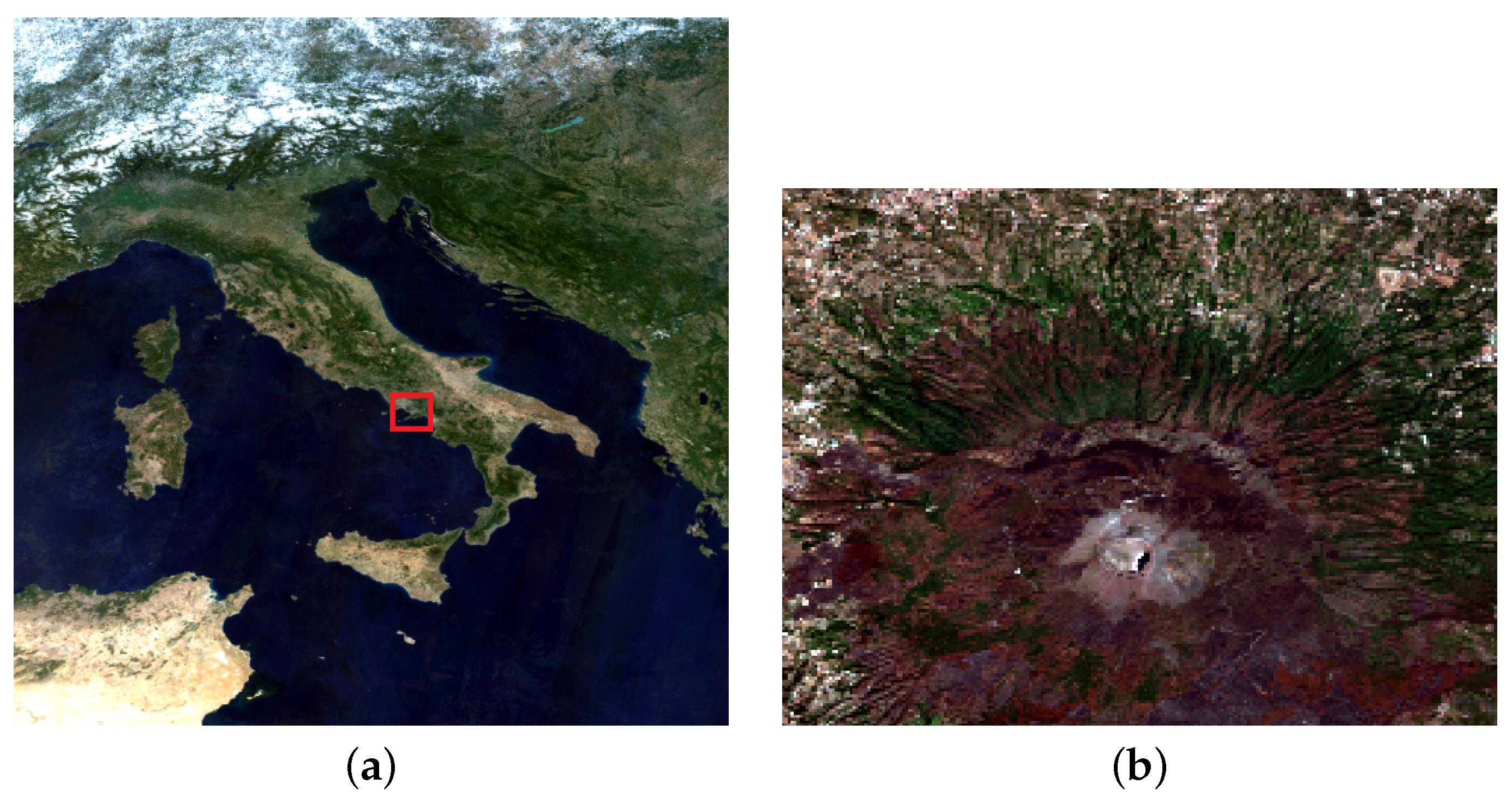
2.1. Study Area
2.2. Remote Sensing Data
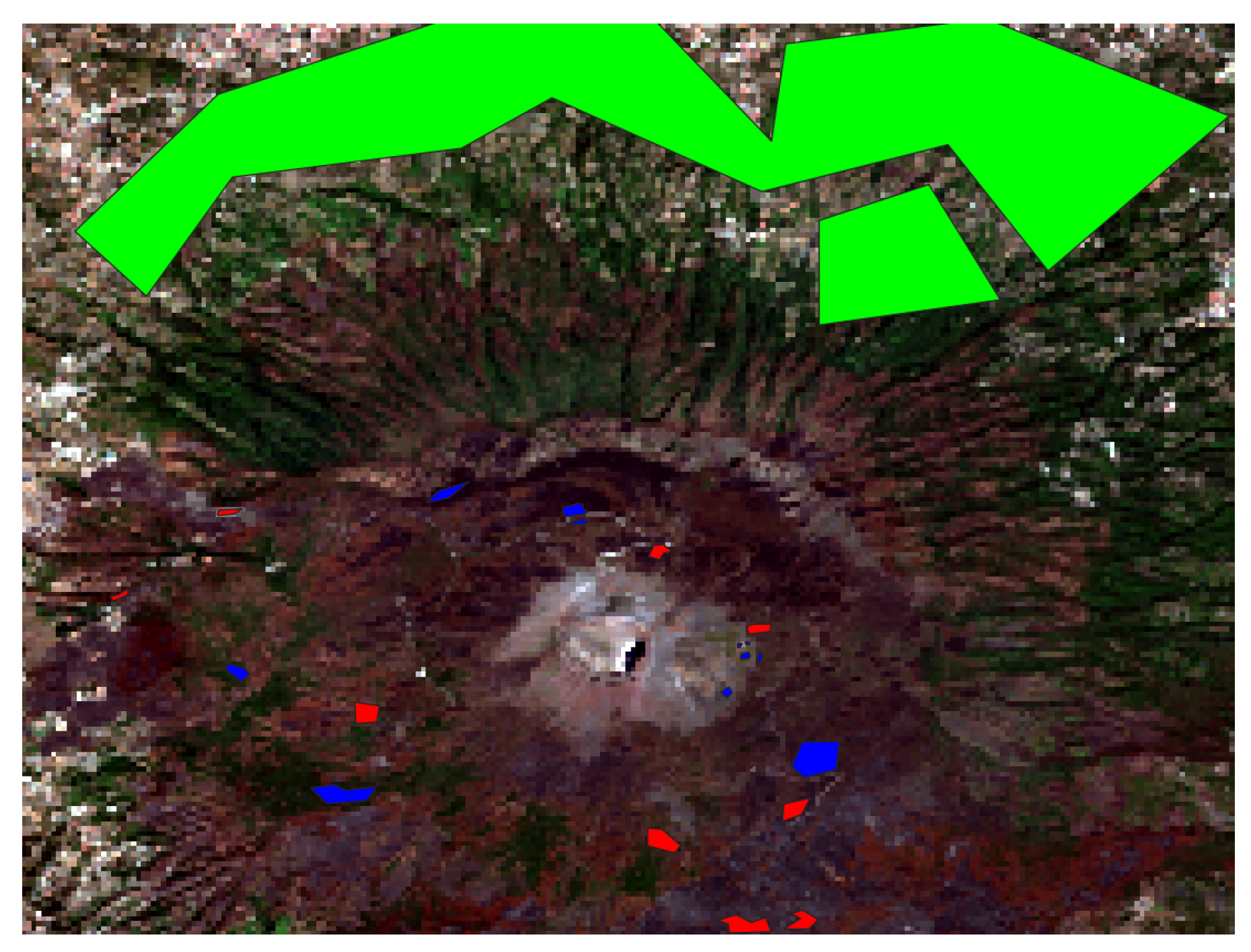
2.3. Soil Sampling
2.4. Soil Chemical Analyses
2.5. Soil Biological Analyses
2.6. Phytotoxicity Assays
3. Proposed Method
3.1. Soil Quality Index (SQI) Calculations
3.2. Selection of the Minimum Dataset ()
3.3. Correlation Coefficient Between Soil Quality Indices and Sentinel-2 Indices
3.4. Relationship Between Biological/Chemical Parameters and Remote Sensing Data
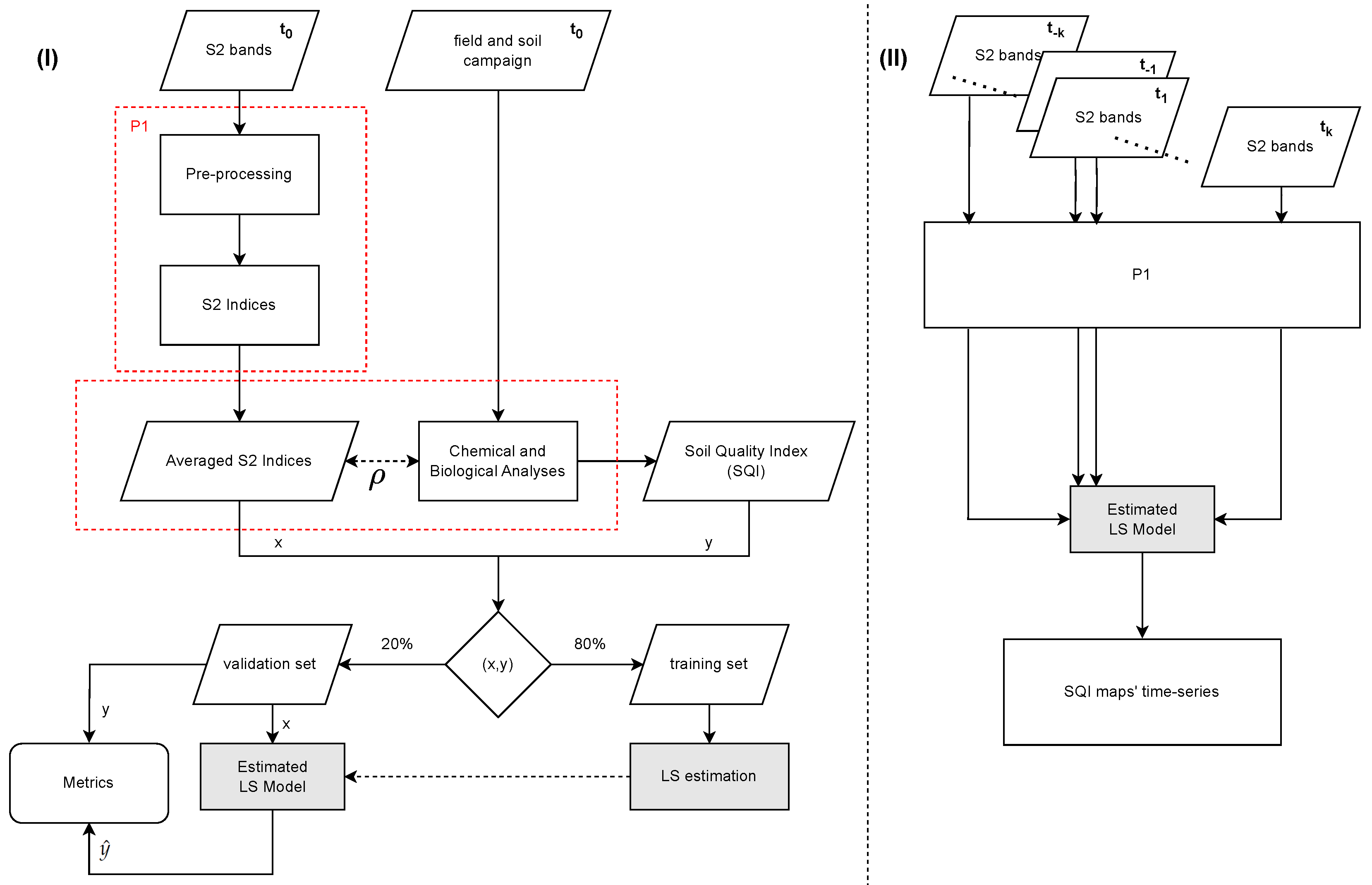
3.5. Least Square (LS) Approach on Remote Sensing Data
3.6. Metrics
4. Results
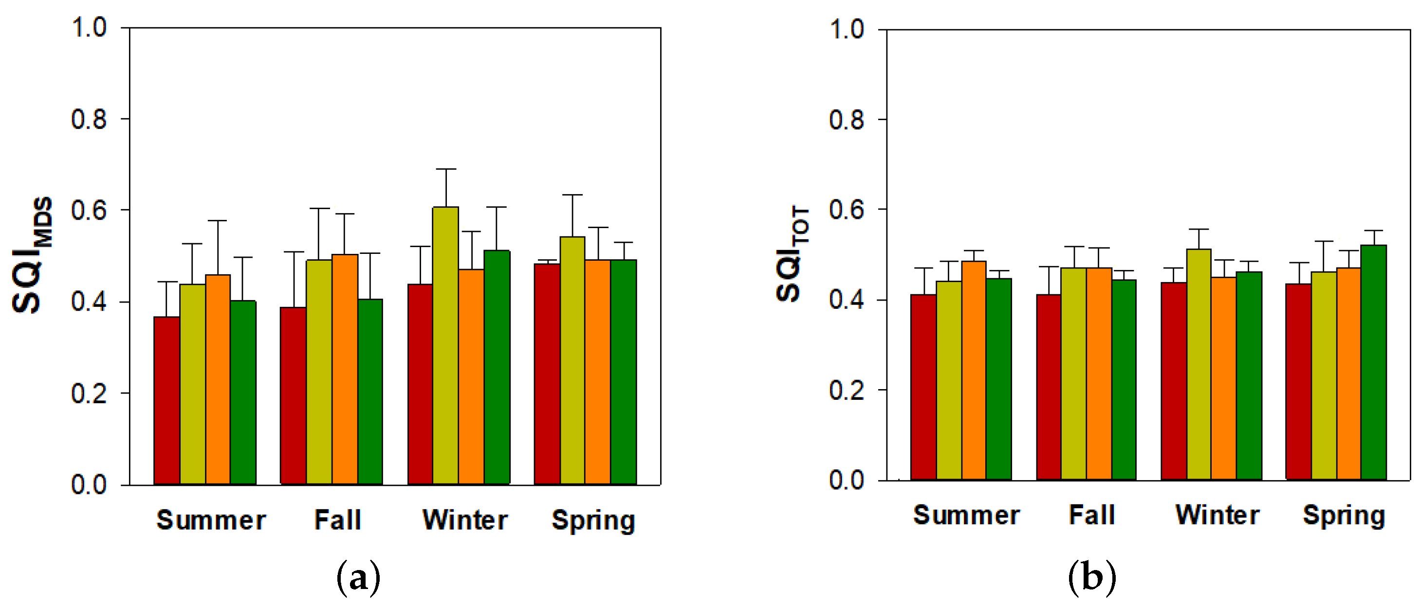
4.1. Soil Quality Index () and Soil Quality Index Minimum Dataset ()
4.2. Numerical Assessment and Visual Inspection
4.3. Time-Series of the Estimated
5. Discussion
6. Conclusions
Author Contributions
Funding
Institutional Review Board Statement
Informed Consent Statement
Data Availability Statement
Conflicts of Interest
Appendix A

| NDI(i,j) | |||||||||
|---|---|---|---|---|---|---|---|---|---|
| i,j = 2,3 | −0.3459 | 0.0708 | −0.2784 | −0.2397 | −0.2921 | −0.2895 | −0.4203 | 0.0968 | 0.0264 |
| i,j = 2,4 | −0.0555 | −0.0057 | −0.083 | −0.0701 | −0.1989 | −0.2301 | −0.0467 | −0.0046 | −0.0446 |
| i,j = 2,5 | −0.3699 | −0.1742 | −0.1884 | −0.0621 | −0.0682 | −0.1941 | −0.3193 | −0.1507 | −0.2253 |
| i,j = 2,6 | −0.4936 | −0.1325 | −0.251 | −0.1438 | −0.0035 | −0.1312 | −0.426 | −0.1185 | −0.1634 |
| i,j = 2,7 | −0.5018 | −0.1627 | −0.2371 | −0.1048 | 0.0477 | −0.1293 | −0.4342 | −0.1361 | −0.1921 |
| i,j = 2,8 | −0.4488 | −0.1699 | −0.1995 | −0.1238 | 0.0291 | −0.1201 | −0.3631 | −0.1583 | −0.1995 |
| i,j = 2,8A | −0.4757 | −0.1665 | −0.2158 | −0.0831 | 0.055 | −0.1053 | −0.403 | −0.1527 | −0.1975 |
| i,j = 2,11 | −0.0856 | −0.3825 | 0.0865 | 0.1023 | 0.0854 | 0.0608 | 0.0216 | −0.3861 | −0.4214 |
| i,j = 2,12 | 0.0867 | −0.4197 | 0.2006 | 0.18 | 0.0994 | 0.1458 | 0.1777 | −0.4323 | −0.4559 |
| i,j = 3,4 | 0.3277 | −0.0809 | 0.2363 | 0.2053 | 0.1664 | 0.1372 | 0.4134 | −0.1078 | −0.0615 |
| i,j = 3,5 | −0.2348 | −0.3061 | −0.0381 | 0.1085 | 0.1476 | −0.0104 | −0.0952 | −0.2952 | −0.3425 |
| i,j = 3,6 | −0.4826 | −0.1782 | −0.2115 | −0.0943 | 0.1092 | −0.0641 | −0.3677 | −0.1726 | −0.2006 |
| i,j = 3,7 | −0.4996 | −0.2057 | −0.2051 | −0.0603 | 0.1527 | −0.0746 | −0.3912 | −0.1833 | −0.2281 |
| i,j = 3,8 | −0.4342 | −0.2148 | −0.1537 | −0.0764 | 0.1356 | −0.0622 | −0.3053 | −0.2112 | −0.2382 |
| i,j = 3,8A | −0.4596 | −0.2157 | −0.1706 | −0.0238 | 0.1743 | −0.0338 | −0.3398 | −0.2103 | −0.2387 |
| i,j = 3,11 | 0.0343 | −0.4743 | 0.2056 | 0.2083 | 0.2117 | 0.1765 | 0.1926 | −0.4899 | −0.5047 |
| i,j = 3,12 | 0.2114 | −0.4892 | 0.3116 | 0.2761 | 0.2032 | 0.2487 | 0.3371 | −0.5124 | −0.5161 |
| i,j = 4,5 | −0.4368 | −0.2042 | −0.2024 | −0.0581 | 0.0077 | −0.1134 | −0.3809 | −0.1751 | −0.2483 |
| i,j = 4,6 | −0.4745 | −0.1186 | −0.2357 | −0.1379 | 0.0349 | −0.0827 | −0.414 | −0.1049 | −0.1406 |
| i,j = 4,7 | −0.4897 | −0.149 | −0.2277 | −0.1049 | 0.0797 | −0.087 | −0.4267 | −0.1228 | −0.1707 |
| i,j = 4,8 | −0.4382 | −0.1576 | −0.1885 | −0.1182 | 0.0653 | −0.0792 | −0.3595 | −0.1463 | −0.1803 |
| i,j = 4,8A | −0.466 | −0.1546 | −0.207 | −0.0842 | 0.0907 | −0.0595 | −0.3978 | −0.1409 | −0.1773 |
| i,j = 4,11 | −0.0943 | −0.4515 | 0.1149 | 0.127 | 0.1499 | 0.1295 | 0.0279 | −0.4559 | −0.488 |
| i,j = 4,12 | 0.1189 | −0.5009 | 0.2567 | 0.2264 | 0.1611 | 0.2279 | 0.2205 | −0.5166 | −0.5354 |
| NDI(i,j) | |||||||||
|---|---|---|---|---|---|---|---|---|---|
| i,j = 5,6 | −0.3942 | −0.0051 | −0.2147 | −0.1717 | 0.0216 | −0.0676 | −0.3533 | −0.0066 | −0.0095 |
| i,j = 5,7 | −0.4338 | −0.0578 | −0.2128 | −0.1286 | 0.0797 | −0.0806 | −0.387 | −0.0395 | −0.0651 |
| i,j = 5,8 | −0.3485 | −0.0728 | −0.1482 | −0.1352 | 0.0636 | −0.0655 | −0.2831 | −0.0761 | −0.0824 |
| i,j = 5,8A | −0.3976 | −0.0598 | −0.1804 | −0.0987 | 0.1026 | −0.0352 | −0.3426 | −0.0614 | −0.0666 |
| i,j = 5,11 | 0.2394 | −0.5341 | 0.3569 | 0.2403 | 0.2252 | 0.2827 | 0.3726 | −0.5684 | −0.5559 |
| i,j = 5,12 | 0.423 | −0.5272 | 0.4545 | 0.3251 | 0.2071 | 0.3463 | 0.5123 | −0.5661 | −0.5454 |
| i,j = 6,7 | −0.3551 | −0.1935 | −0.1051 | 0.079 | 0.2277 | −0.1179 | −0.3159 | −0.1154 | −0.2086 |
| i,j = 6,8 | −0.0709 | −0.1608 | 0.0703 | 0.0119 | 0.1174 | −0.0323 | 0.0089 | −0.1677 | −0.1767 |
| i,j = 6,8A | −0.0106 | −0.2792 | 0.1872 | 0.3992 | 0.4235 | 0.2265 | 0.0659 | −0.2826 | −0.2917 |
| i,j = 6,11 | 0.4583 | −0.3486 | 0.3961 | 0.2913 | 0.1362 | 0.2362 | 0.5132 | −0.3702 | −0.3584 |
| i,j = 6,12 | 0.5023 | −0.3549 | 0.4232 | 0.3154 | 0.1284 | 0.271 | 0.537 | −0.3804 | −0.3643 |
| i,j = 7,8 | 0.1379 | −0.0485 | 0.1344 | −0.033 | −0.0134 | 0.0289 | 0.1954 | −0.1017 | −0.0558 |
| i,j = 7,8A | 0.3725 | 0.006 | 0.2475 | 0.2027 | 0.0613 | 0.2345 | 0.3854 | −0.0801 | 0.0133 |
| i,j = 7,11 | 0.5056 | −0.29 | 0.3955 | 0.2586 | 0.0817 | 0.2422 | 0.5485 | −0.326 | −0.2961 |
| i,j = 7,12 | 0.5331 | −0.3079 | 0.4193 | 0.2884 | 0.0862 | 0.2715 | 0.5583 | −0.3439 | −0.3148 |
| i,j = 8,8A | 0.0667 | 0.0518 | 0.0009 | 0.1441 | 0.0463 | 0.1022 | 0.0161 | 0.0576 | 0.063 |
| i,j = 8,11 | 0.4596 | −0.2752 | 0.3506 | 0.2723 | 0.0873 | 0.2362 | 0.4826 | −0.2929 | −0.279 |
| i,j = 8,12 | 0.503 | −0.2993 | 0.3901 | 0.2996 | 0.091 | 0.2684 | 0.5156 | −0.322 | −0.3042 |
| i,j = 8A,11 | 0.4841 | −0.3206 | 0.3868 | 0.2453 | 0.0761 | 0.2188 | 0.5276 | −0.3426 | −0.3291 |
| i,j = 8A,12 | 0.5211 | −0.332 | 0.4161 | 0.2842 | 0.0833 | 0.2592 | 0.5466 | −0.358 | −0.3404 |
| i,j = 11,12 | 0.5846 | −0.3574 | 0.4723 | 0.3577 | 0.112 | 0.3424 | 0.5798 | −0.3923 | −0.3651 |
| NDI(i,j) | WC | pH | C | N | OM |
|---|---|---|---|---|---|
| i,j = 2,3 | −0.0122 | −0.0683 | −0.2253 | 0.1592 | −0.3458 |
| i,j = 2,4 | 0.2359 | 0.3398 | −0.1077 | 0.4277 | −0.349 |
| i,j = 2,5 | −0.1246 | 0.1693 | −0.4565 | 0.1665 | −0.3708 |
| i,j = 2,6 | −0.3161 | 0.023 | −0.356 | 0.0783 | −0.2815 |
| i,j = 2,7 | −0.372 | 0.0592 | −0.3155 | 0.1217 | −0.252 |
| i,j = 2,8 | −0.3016 | 0.1276 | −0.3317 | 0.1946 | −0.3175 |
| i,j = 2,8A | −0.328 | 0.0575 | −0.3383 | 0.1084 | −0.2808 |
| i,j = 2,11 | 0.0106 | 0.2193 | −0.4314 | 0.2316 | −0.4246 |
| i,j = 2,12 | 0.1323 | 0.2076 | −0.403 | 0.2169 | −0.3919 |
| i,j = 3,4 | 0.1866 | 0.3179 | 0.1685 | 0.1456 | 0.1188 |
| i,j = 3,5 | −0.1751 | 0.2987 | −0.492 | 0.084 | −0.2502 |
| i,j = 3,6 | −0.4058 | 0.0547 | −0.3989 | 0.0006 | −0.2367 |
| i,j = 3,7 | −0.4621 | 0.0931 | −0.3492 | 0.0638 | −0.21 |
| i,j = 3,8 | −0.3895 | 0.1737 | −0.3801 | 0.1452 | −0.2975 |
| i,j = 3,8A | −0.4136 | 0.0958 | −0.3773 | 0.0437 | −0.2381 |
| i,j = 3,11 | 0.0039 | 0.2804 | −0.4592 | 0.1892 | −0.3807 |
| i,j = 3,12 | 0.1438 | 0.2462 | −0.3929 | 0.1756 | −0.3282 |
| i,j = 4,5 | −0.2808 | 0.0198 | −0.5261 | −0.0308 | −0.2832 |
| i,j = 4,6 | −0.3682 | −0.0767 | −0.3416 | −0.0452 | −0.1964 |
| i,j = 4,7 | −0.419 | −0.0343 | −0.3085 | 0.0095 | −0.1791 |
| i,j = 4,8 | −0.3571 | 0.0347 | −0.3293 | 0.0795 | −0.2451 |
| i,j = 4,8A | −0.3826 | −0.042 | −0.3306 | −0.0104 | −0.1994 |
| i,j = 4,11 | −0.0591 | 0.1446 | −0.4984 | 0.1385 | −0.4071 |
| i.j = 4,12 | 0.102 | 0.1472 | −0.4594 | 0.1412 | −0.3813 |
| NDI(i,j) | WC | pH | C | N | OM |
|---|---|---|---|---|---|
| i,j = 5,6 | −0.3499 | −0.1339 | −0.1754 | −0.0701 | −0.1367 |
| i,j = 5,7 | −0.4264 | −0.0717 | −0.1609 | 0.0059 | −0.1299 |
| i,j = 5,8 | −0.3357 | 0.0251 | −0.1983 | 0.1005 | −0.2258 |
| i,j = 5,8A | −0.3839 | −0.0866 | −0.1781 | −0.0212 | −0.1525 |
| i,j = 5,11 | 0.1501 | 0.2056 | −0.3495 | 0.2388 | −0.4035 |
| i,j = 5,12 | 0.3017 | 0.1732 | −0.2662 | 0.2005 | −0.3057 |
| i,j = 6,7 | −0.4716 | 0.181 | −0.0308 | 0.2705 | −0.0578 |
| i,j = 6,8 | −0.1454 | 0.3387 | −0.1598 | 0.3918 | −0.3134 |
| i,j = 6,8A | −0.1794 | 0.2542 | −0.0284 | 0.262 | −0.1025 |
| i,j = 6,11 | 0.3653 | 0.2396 | −0.081 | 0.215 | −0.1384 |
| i,j = 6,12 | 0.3993 | 0.1865 | −0.069 | 0.1752 | −0.1175 |
| i,j = 7,8 | 0.1277 | 0.2363 | −0.1447 | 0.2358 | −0.2827 |
| i,j = 7,8A | 0.3752 | −0.0102 | 0.0121 | −0.1011 | −0.0112 |
| i,j = 7,11 | 0.4421 | 0.188 | −0.0691 | 0.1468 | −0.1166 |
| i,j = 7,12 | 0.4533 | 0.1486 | −0.0591 | 0.1253 | −0.1031 |
| i,j = 8,8A | 0.0801 | −0.2421 | 0.1525 | −0.2904 | 0.2767 |
| i,j = 8,11 | 0.3982 | 0.1065 | −0.0186 | 0.0641 | −0.0176 |
| i,j = 8,12 | 0.4234 | 0.0919 | −0.0253 | 0.0662 | −0.0359 |
| i,j = 8A,11 | 0.4138 | 0.2075 | −0.0774 | 0.1818 | −0.1284 |
| i,j = 8A,12 | 0.4343 | 0.1585 | −0.0651 | 0.1481 | −0.1112 |
| i,j = 11,12 | 0.4527 | 0.0652 | −0.0544 | 0.0775 | −0.0703 |
| NDI(i,j) | Resp | ||||||
|---|---|---|---|---|---|---|---|
| i,j = 2,3 | −0.2018 | 0.0941 | 0.1595 | 0.2 | 0.0838 | 0.2667 | −0.1243 |
| i,j = 2,4 | 0.0556 | 0.0228 | 0.1599 | 0.1951 | −0.019 | 0.0406 | −0.3033 |
| i,j = 2,5 | −0.4168 | 0.2055 | 0.0223 | 0.1192 | −0.1579 | 0.1733 | 0.1637 |
| i,j = 2,6 | −0.5545 | 0.2748 | 0.1786 | 0.2166 | −0.1082 | 0.1125 | 0.3069 |
| i,j = 2,7 | −0.5548 | 0.2474 | 0.2295 | 0.2393 | −0.1366 | 0.0295 | 0.3523 |
| i,j = 2,8 | −0.5082 | 0.219 | 0.2172 | 0.2296 | −0.1507 | −0.0081 | 0.3299 |
| i,j = 2,8A | −0.5568 | 0.2531 | 0.1354 | 0.171 | −0.1425 | 0.0764 | 0.3589 |
| i,j = 2,11 | −0.2015 | 0.2697 | −0.016 | 0.0586 | −0.3787 | 0.0833 | 0.285 |
| i,j = 2,12 | −0.0524 | 0.2458 | −0.0747 | 0.0169 | −0.4236 | 0.1138 | 0.227 |
| i,j = 3,4 | 0.2531 | −0.0844 | −0.0533 | −0.071 | −0.1044 | −0.255 | −0.0625 |
| i,j = 3,5 | −0.4247 | 0.2222 | −0.1045 | 0.0001 | −0.2942 | 0.0181 | 0.3195 |
| i,j = 3,6 | −0.6053 | 0.3183 | 0.1515 | 0.1827 | −0.1531 | 0.0366 | 0.4084 |
| i,j = 3,7 | −0.5999 | 0.2822 | 0.2211 | 0.2183 | −0.1785 | −0.0505 | 0.4473 |
| i,j = 3,8 | −0.5486 | 0.2457 | 0.2006 | 0.2049 | −0.1955 | −0.0921 | 0.4341 |
| i,j = 3,8A | −0.6042 | 0.2914 | 0.1007 | 0.1298 | −0.1913 | −0.0034 | 0.4615 |
| i,j = 3,11 | −0.1612 | 0.2906 | −0.0762 | −0.003 | −0.4754 | −0.0084 | 0.3615 |
| i,j = 3,12 | 0.0063 | 0.2441 | −0.1283 | −0.0397 | −0.4981 | 0.0363 | 0.2773 |
| i,j = 4,5 | −0.5463 | 0.2439 | −0.0486 | 0.0514 | −0.1769 | 0.2005 | 0.3217 |
| i,j = 4,6 | −0.5498 | 0.2688 | 0.1351 | 0.1617 | −0.0913 | 0.1112 | 0.3547 |
| i,j = 4,7 | −0.5544 | 0.2476 | 0.1925 | 0.1925 | −0.1201 | 0.033 | 0.393 |
| i,j = 4,8 | −0.5124 | 0.2177 | 0.1799 | 0.1841 | −0.1352 | −0.0024 | 0.3761 |
| i,j = 4,8A | −0.5619 | 0.2531 | 0.101 | 0.1255 | −0.1274 | 0.0779 | 0.4084 |
| i,j = 4,11 | −0.2613 | 0.3167 | −0.0523 | 0.0249 | −0.443 | 0.0957 | 0.4015 |
| i,j = 4,12 | −0.074 | 0.2843 | −0.1209 | −0.0211 | −0.5025 | 0.1315 | 0.3247 |
| NDI(i,j) | Resp | ||||||
|---|---|---|---|---|---|---|---|
| i,j = 5,6 | −0.4112 | 0.2419 | 0.2252 | 0.2007 | 0.0158 | 0.0466 | 0.2599 |
| i,j = 5,7 | −0.4387 | 0.2241 | 0.2976 | 0.2430 | −0.0336 | −0.0475 | 0.3253 |
| i,j = 5,8 | −0.3723 | 0.172 | 0.2606 | 0.2179 | −0.058 | −0.0906 | 0.3019 |
| i,j = 5,8A | −0.4491 | 0.2347 | 0.1798 | 0.1558 | −0.0382 | 0.0070 | 0.3541 |
| i,j = 5,11 | 0.0749 | 0.2815 | −0.0160 | 0.018 | −0.5454 | −0.0146 | 0.338 |
| i,j = 5,12 | 0.2411 | 0.2052 | −0.1080 | −0.0444 | −0.5463 | 0.0441 | 0.2139 |
| i,j = 6,7 | −0.2927 | 0.0512 | 0.3994 | 0.2639 | −0.1701 | −0.3459 | 0.3893 |
| i,j = 6,8 | −0.0883 | −0.0665 | 0.1827 | 0.1256 | −0.1660 | −0.3275 | 0.2262 |
| i,j = 6,8A | −0.1952 | −0.0100 | −0.2552 | −0.2484 | −0.2758 | −0.2055 | 0.444 |
| i,j = 6,11 | 0.3608 | −0.0076 | −0.1745 | −0.1353 | −0.3721 | −0.0537 | 0.0184 |
| i,j = 6,12 | 0.3869 | −0.0015 | −0.1913 | −0.1362 | −0.3794 | 0.0024 | 0.0051 |
| i,j = 7,8 | 0.0822 | −0.0979 | −0.0510 | −0.0288 | −0.0676 | −0.1282 | −0.0049 |
| i,j = 7,8A | 0.1723 | −0.0618 | −0.6109 | −0.4609 | −0.0166 | 0.2223 | −0.0607 |
| i,j = 7,11 | 0.3996 | −0.0189 | −0.2456 | −0.1807 | −0.3169 | 0.0215 | −0.0553 |
| i,j = 7,12 | 0.4155 | −0.0109 | −0.2429 | −0.1701 | −0.3349 | 0.0566 | −0.0506 |
| i,j = 8,8A | 0.013 | 0.064 | −0.2846 | −0.2246 | 0.0584 | 0.2506 | −0.0312 |
| i,j = 8,11 | 0.3719 | 0.0156 | −0.2279 | −0.17 | −0.2956 | 0.0662 | −0.0538 |
| i,j = 8,12 | 0.3986 | 0.0149 | −0.2341 | −0.1663 | −0.3216 | 0.0869 | −0.0483 |
| i,j = 8A,11 | 0.4109 | −0.0088 | −0.1469 | −0.1064 | −0.3458 | −0.0209 | −0.0521 |
| i,j = 8A,12 | 0.4228 | −0.0005 | −0.1753 | −0.1185 | −0.3578 | 0.0288 | −0.0470 |
| i,j = 11,12 | 0.4318 | 0.0225 | −0.2265 | −0.1361 | −0.3834 | 0.1240 | −0.0229 |
References
- Cabral, A.I.; Saito, C.; Pereira, H.; Laques, A.E. Deforestation pattern dynamics in protected areas of the Brazilian Legal Amazon using remote sensing data. Appl. Geogr. 2018, 100, 101–115. [Google Scholar] [CrossRef]
- Mikeladze, G.; Gavashelishvili, A.; Akobia, I.; Metreveli, V. Estimation of forest cover change using Sentinel-2 multi-spectral imagery in Georgia (the Caucasus). IForest-Biogeosci. For. 2020, 13, 329. [Google Scholar] [CrossRef]
- Turco, M.; von Hardenberg, J.; AghaKouchak, A.; Llasat, M.C.; Provenzale, A.; Trigo, R.M. On the key role of droughts in the dynamics of summer fires in Mediterranean Europe. Sci. Rep. 2017, 7, 81. [Google Scholar] [CrossRef]
- Curtis, P.G.; Slay, C.M.; Harris, N.L.; Tyukavina, A.; Hansen, M.C. Classifying drivers of global forest loss. Science 2018, 361, 1108–1111. [Google Scholar] [CrossRef]
- Santorufo, L.; Memoli, V.; Panico, S.C.; Esposito, F.; Vitale, L.; Di Natale, G.; Trifuoggi, M.; Barile, R.; De Marco, A.; Maisto, G. Impact of Anthropic Activities on Soil Quality under Different Land Uses. Int. J. Environ. Res. Public Health 2021, 18, 8423. [Google Scholar] [CrossRef]
- Jain, T.B.; Pilliod, D.S.; Graham, R.T.; Lentile, L.B.; Sandquist, J.E. Index for characterizing post-fire soil environments in temperate coniferous forests. Forests 2012, 3, 445–466. [Google Scholar] [CrossRef]
- Santorufo, L.; Memoli, V.; Panico, S.C.; Santini, G.; Barile, R.; Giarra, A.; Di Natale, G.; Trifuoggi, M.; De Marco, A.; Maisto, G. Combined Effects of Wildfire and Vegetation Cover Type on Volcanic Soil (Functions and Properties) in a Mediterranean Region: Comparison of Two Soil Quality Indices. Int. J. Environ. Res. Public Health 2021, 18, 5926. [Google Scholar] [CrossRef]
- Zavala, L.M.M.; de Celis Silvia, R.; López, A.J. How wildfires affect soil properties. A brief review. Cuad. Investig. Geográfica/Geogr. Res. Lett. 2014, 40, 311–331. [Google Scholar] [CrossRef]
- Certini, G.; Moya, D.; Lucas-Borja, M.E.; Mastrolonardo, G. The impact of fire on soil-dwelling biota: A review. For. Ecol. Manag. 2021, 488, 118989. [Google Scholar] [CrossRef]
- Forkuor, G.; Dimobe, K.; Serme, I.; Tondoh, J.E. Landsat-8 vs. Sentinel-2: Examining the added value of sentinel-2’s red-edge bands to land-use and land-cover mapping in Burkina Faso. GIScience Remote Sens. 2018, 55, 331–354. [Google Scholar] [CrossRef]
- Puletti, N.; Chianucci, F.; Castaldi, C. Use of Sentinel-2 for forest classification in Mediterranean environments. Ann. Silvic. Res 2017, 42, 32–38. [Google Scholar]
- Gargiulo, M.; Dell’Aglio, D.A.; Iodice, A.; Riccio, D.; Ruello, G. Integration of Sentinel-1 and Sentinel-2 Data for Land Cover Mapping Using W-Net. Sensors 2020, 20, 2969. [Google Scholar] [CrossRef]
- Pause, M.; Schweitzer, C.; Rosenthal, M.; Keuck, V.; Bumberger, J.; Dietrich, P.; Heurich, M.; Jung, A.; Lausch, A. In situ/remote sensing integration to assess forest health—A review. Remote Sens. 2016, 8, 471. [Google Scholar] [CrossRef]
- Kaufman, Y.J.; Justice, C.O.; Flynn, L.P.; Kendall, J.D.; Prins, E.M.; Giglio, L.; Ward, D.E.; Menzel, W.P.; Setzer, A.W. Potential global fire monitoring from EOS-MODIS. J. Geophys. Res. Atmos. 1998, 103, 32215–32238. [Google Scholar] [CrossRef]
- Schroeder, W.; Oliva, P.; Giglio, L.; Csiszar, I.A. The New VIIRS 375 m active fire detection data product: Algorithm description and initial assessment. Remote Sens. Environ. 2014, 143, 85–96. [Google Scholar] [CrossRef]
- Laneve, G.; Pampanoni, V.; Shaik, R.U. The Daily Fire Hazard Index: A Fire Danger Rating Method for Mediterranean Areas. Remote Sens. 2020, 12, 2356. [Google Scholar] [CrossRef]
- Gargiulo, M.; Dell’Aglio, D.A.G.; Iodice, A.; Riccio, D.; Ruello, G. A CNN-Based Super-Resolution Technique for Active Fire Detection on Sentinel-2 Data. In Proceedings of the 2019 PhotonIcs & Electromagnetics Research Symposium-Spring (PIERS-Spring), Rome, Italy, 17–20 June 2019; IEEE: Piscataway, NJ, USA, 2019; pp. 418–426. [Google Scholar]
- Huang, H.; Roy, D.; Boschetti, L.; Zhang, H.; Yan, L.; Kumar, S.; Gomez-Dans, J.; Li, J. Separability Analysis of Sentinel-2A Multi-Spectral Instrument (MSI) Data for Burned Area Discrimination. Remote Sens. 2016, 8, 873. [Google Scholar] [CrossRef]
- Mura, M.; Bottalico, F.; Giannetti, F.; Bertani, R.; Giannini, R.; Mancini, M.; Orlandini, S.; Travaglini, D.; Chirici, G. Exploiting the capabilities of the Sentinel-2 multi spectral instrument for predicting growing stock volume in forest ecosystems. Int. J. Appl. Earth Obs. Geoinf. 2018, 66, 126–134. [Google Scholar] [CrossRef]
- Cuevas-González, M.; Gerard, F.; Balzter, H.; Riano, D. Analysing forest recovery after wildfire disturbance in boreal Siberia using remotely sensed vegetation indices. Glob. Change Biol. 2009, 15, 561–577. [Google Scholar] [CrossRef]
- Huete, A.R.; Liu, H.; van Leeuwen, W.J. The use of vegetation indices in forested regions: Issues of linearity and saturation. In Proceedings of the IGARSS’97, 1997 IEEE International Geoscience and Remote Sensing Symposium Proceedings, Remote Sensing—A Scientific Vision for Sustainable Development, Singapore, 3–8 August 1997; IEEE: Piscataway, NJ, USA, 1997; Volume 4, pp. 1966–1968. [Google Scholar]
- Semeraro, T.; Vacchiano, G.; Aretano, R.; Ascoli, D. Application of vegetation index time series to value fire effect on primary production in a Southern European rare wetland. Ecol. Eng. 2019, 134, 9–17. [Google Scholar] [CrossRef]
- Lentile, L.; Holden, Z.; Smith, A.M.S.; Falkowski, M.; Hudak, A.; A Morgan, P.; Lewis, S.; Gessler, P.; Benson, N. Remote sensing techniques to assess active fire characteristics and post-fire effects. Int. J. Wildland Fire 2006, 15, 319–345. [Google Scholar] [CrossRef]
- Schroeder, W.; Oliva, P.; Giglio, L.; Quayle, B.; Lorenz, E.; Morelli, F. Active fire detection using Landsat-8/OLI data. Remote Sens. Environ. 2016, 185, 210–220. [Google Scholar] [CrossRef]
- Barducci, A.; Guzzi, D.; Marcoionni, P.; Pippi, I. Infrared detection of active fires and burnt areas: Theory and observations. Infrared Phys. Technol. 2002, 43, 119–125. [Google Scholar] [CrossRef]
- Kuenzer, C.; Dech, S. Thermal infrared remote sensing. Remote Sens. Digit. Image Processing. Doi 2013, 10, 978–994. [Google Scholar]
- Henry, M.C.; Maingi, J.K. Evaluating Landsat-and Sentinel-2-Derived Burn Indices to Map Burn Scars in Chyulu Hills, Kenya. Fire 2024, 7, 472. [Google Scholar] [CrossRef]
- Gargiulo, M.; Iodice, A.; Riccio, D.; Ruello, G. Sentinel-1 Time-Series Analysis for Fires Monitoring using Google Earth Engine Tools. In Proceedings of the 2021 IEEE 6th International Forum on Research and Technology for Society and Industry (RTSI), Naples, Italy, 6–9 September 2021; IEEE: Piscataway, NJ, USA, 2021; pp. 232–236. [Google Scholar]
- Memoli, V.; Esposito, F.; Santorufo, L.; Panico, S.C.; Trifuoggi, M.; Di Natale, G.; Maisto, G. Relationships between leaf exposure time to air pollution and metal and particulate matter accumulation for holm oak leaves. Water Air Soil Pollut. 2020, 231, 529. [Google Scholar] [CrossRef]
- Alessio, G.; De Lucia, M. Promotion and development of protected volcanic areas through field-based environmental communication activities: The ‘Gran Cono’tour in the Vesuvius National Park (Italy). Geoheritage 2017, 9, 435–442. [Google Scholar] [CrossRef]
- Filipponi, F. Exploitation of sentinel-2 time series to map burned areas at the national level: A case study on the 2017 italy wildfires. Remote Sens. 2019, 11, 622. [Google Scholar] [CrossRef]
- Panico, S.C.; Memoli, V.; Santorufo, L.; Esposito, F.; De Marco, A.; Barile, R.; Maisto, G. Linkage between site features and soil characteristics within a Mediterranean volcanic area. Front. For. Glob. Change 2021, 3, 621231. [Google Scholar] [CrossRef]
- Saulino, L.; Rita, A.; Migliozzi, A.; Maffei, C.; Allevato, E.; Garonna, A.P.; Saracino, A. Detecting burn severity across mediterranean forest types by coupling medium-spatial resolution satellite imagery and field data. Remote Sens. 2020, 12, 741. [Google Scholar] [CrossRef]
- Memoli, V.; Santorufo, L.; Santini, G.; Musella, P.; Barile, R.; De Marco, A.; Di Natale, G.; Trifuoggi, M.; Maisto, G. Role of Seasonality and Fire in Regulating the Enzymatic Activities in Soils Covered by Different Vegetation in a Mediterranean Area. Appl. Sci. 2021, 11, 8342. [Google Scholar] [CrossRef]
- San Miguel Ayanz, J.; Barbosa, P.; Schmuck, G.; Liberta, G.; Schulte, E.; Gitas, I. Towards a Coherent Forest Fire Information System in Europe: The European Forest Fire Information System (EFFIS); Millpress: Rotterdam, The Netherlands, 2002. [Google Scholar]
- McFerren, G.; Frost, P. Southern african advanced fire information system. In Proceedings of the 6th International Information Systems for Crisis Response and Management (ISCRAM) Conference, Gothenburg, Sweden, 10–13 May 2009. [Google Scholar]
- Marino, E.; Yáñez, L.; Guijarro, M.; Madrigal, J.; Senra, F.; Rodríguez, S.; Tomé, J.L. Transferability of Empirical Models Derived from Satellite Imagery for Live Fuel Moisture Content Estimation and Fire Risk Prediction. Fire 2024, 7, 276. [Google Scholar] [CrossRef]
- Adams, J.B.; Sabol, D.E.; Kapos, V.; Almeida Filho, R.; Roberts, D.A.; Smith, M.O.; Gillespie, A.R. Classification of multispectral images based on fractions of endmembers: Application to land-cover change in the Brazilian Amazon. Remote Sens. Environ. 1995, 52, 137–154. [Google Scholar] [CrossRef]
- Pal, M.K.; Rasmussen, T.M.; Abdolmaleki, M. Multiple Multi-Spectral Remote Sensing Data Fusion and Integration for Geological Mapping. In Proceedings of the 2019 10th Workshop on Hyperspectral Imaging and Signal Processing: Evolution in Remote Sensing (WHISPERS), Amsterdam, The Netherlands, 24–26 September 2019; IEEE: Piscataway, NJ, USA, 2019; pp. 1–5. [Google Scholar]
- Carlson, T.N.; Ripley, D.A. On the relation between NDVI, fractional vegetation cover, and leaf area index. Remote Sens. Environ. 1997, 62, 241–252. [Google Scholar] [CrossRef]
- Maselli, F.; Chiesi, M.; Pieri, M. A new method to enhance the spatial features of multitemporal NDVI image series. IEEE Trans. Geosci. Remote Sens. 2019, 57, 4967–4979. [Google Scholar] [CrossRef]
- Manzo, C.; Mei, A.; Fontinovo, G.; Allegrini, A.; Bassani, C. Integrated remote sensing for multi-temporal analysis of anthropic activities in the south-east of Mt. Vesuvius National Park. J. Afr. Earth Sci. 2016, 122, 63–78. [Google Scholar] [CrossRef]
- Rokni, K.; Ahmad, A.; Solaimani, K.; Hazini, S. A new approach for detection of surface water changes based on principal component analysis of multitemporal normalized difference water index. J. Coast. Res. 2016, 32, 443–451. [Google Scholar]
- Gargiulo, M.; Mazza, A.; Gaetano, R.; Ruello, G.; Scarpa, G. A CNN-based fusion method for super-resolution of Sentinel-2 data. In Proceedings of the IGARSS 2018–2018 IEEE International Geoscience and Remote Sensing Symposium, Valencia, Spain, 22–27 July 2018; IEEE: Piscataway, NJ, USA, 2018; pp. 4713–4716. [Google Scholar]
- McFeeters, S.K. The use of the Normalized Difference Water Index (NDWI) in the delineation of open water features. Int. J. Remote Sens. 1996, 17, 1425–1432. [Google Scholar] [CrossRef]
- Atun, R.; Kalkan, K.; Gürsoy, Ö. Determining the forest fire risk with sentinel 2 images. Turk. J. Geosci. 2020, 1, 22–26. [Google Scholar]
- Sánchez Sánchez, Y.; Martínez-Graña, A.; Santos Francés, F.; Mateos Picado, M. Mapping wildfire ignition probability using sentinel 2 and LiDAR (Jerte Valley, Caceres, Spain). Sensors 2018, 18, 826. [Google Scholar] [CrossRef]
- Pádua, L.; Guimarães, N.; Adão, T.; Sousa, A.; Peres, E.; Sousa, J.J. Effectiveness of Sentinel-2 in Multi-Temporal Post-Fire Monitoring When Compared with UAV Imagery. ISPRS Int. J. Geo-Inf. 2020, 9, 225. [Google Scholar] [CrossRef]
- Evangelides, C.; Nobajas, A. Red-Edge Normalised Difference Vegetation Index (NDVI705) from Sentinel-2 imagery to assess post-fire regeneration. Remote Sens. Appl. Soc. Environ. 2020, 17, 100283. [Google Scholar] [CrossRef]
- Smiraglia, D.; Filipponi, F.; Mandrone, S.; Tornato, A.; Taramelli, A. Agreement Index for Burned Area Mapping: Integration of Multiple Spectral Indices Using Sentinel-2 Satellite Images. Remote Sens. 2020, 12, 1862. [Google Scholar] [CrossRef]
- Farhadi, H.; Ebadi, H.; Kiani, A. Badi: A novel burned area detection index for sentinel-2 imagery using google earth engine platform. ISPRS Ann. Photogramm. Remote Sens. Spat. Inf. Sci. 2023, 10, 179–186. [Google Scholar] [CrossRef]
- Main-Knorn, M.; Pflug, B.; Louis, J.; Debaecker, V.; Müller-Wilm, U.; Gascon, F. Sen2Cor for sentinel-2. In Proceedings of the Image and Signal Processing for Remote Sensing XXIII. International Society for Optics and Photonics, Warsaw, Poland, 4 October 2017; Volume 10427, p. 1042704. [Google Scholar]
- Memoli, V.; Eymar, E.; García-Delgado, C.; Esposito, F.; Santorufo, L.; De Marco, A.; Barile, R.; Maisto, G. Total and fraction content of elements in volcanic soil: Natural or anthropogenic derivation. Sci. Total Environ. 2018, 625, 16–26. [Google Scholar] [CrossRef] [PubMed]
- Santorufo, L.; Memoli, V.; Panico, S.C.; Santini, G.; Barile, R.; Di Natale, G.; Trifuoggi, M.; De Marco, A.; Maisto, G. Early post-fire changes in properties of Andosols within a Mediterranean area. Geoderma 2021, 394, 115016. [Google Scholar] [CrossRef]
- Pribyl, D.W. A critical review of the conventional SOC to SOM conversion factor. Geoderma 2010, 156, 75–83. [Google Scholar] [CrossRef]
- Waske, B.; van der Linden, S. Classifying Multilevel Imagery From SAR and Optical Sensors by Decision Fusion. IEEE Trans. Geosci. Remote Sens. 2008, 46, 1457–1466. [Google Scholar] [CrossRef]
- Degens, B.P.; Schipper, L.A.; Sparling, G.P.; Vojvodic-Vukovic, M. Decreases in organic C reserves in soils can reduce the catabolic diversity of soil microbial communities. Soil Biol. Biochem. 2000, 32, 189–196. [Google Scholar] [CrossRef]
- Sundman, V.; Sivelä, S. A comment on the membrane filter technique for estimation of length of fungal hyphae in soil. Soil Biol. Biochem. 1978, 10, 399–401. [Google Scholar] [CrossRef]
- Olson, F. Quantitative estimates of filamentous algae. Trans. Am. Microsc. Soc. 1950, 69, 272–279. [Google Scholar] [CrossRef]
- Froment, A. Soil respiration in a mixed oak forest. Oikos 1972, 23, 273–277. [Google Scholar] [CrossRef]
- Anderson, J.P.; Domsch, K.H. A physiological method for the quantitative measurement of microbial biomass in soils. Soil Biol. Biochem. 1978, 10, 215–221. [Google Scholar] [CrossRef]
- Adam, G.; Duncan, H. Development of a sensitive and rapid method for the measurement of total microbial activity using fluorescein diacetate (FDA) in a range of soils. Soil Biol. Biochem. 2001, 33, 943–951. [Google Scholar] [CrossRef]
- Tabatabai, M.A.; Bremner, J.M. Use of p-nitrophenyl phosphate for assay of soil phosphatase activity. Soil Biol. Biochem. 1969, 1, 301–307. [Google Scholar] [CrossRef]
- Tabatabai, M. Soil enzymes. In Methods of Soil Analysis: Part 2 Microbiological and Biochemical Properties; The American Society of Agronomy: Madison, WI, USA, 1994; Volume 5, pp. 775–833. [Google Scholar]
- EPA. Ecological effects test guidelines. In Seed Germination/Root Elongation Toxicity Test; OPPTS 850.4200; EPA-712-C-96-154; EPA: Washington, DC, USA, 1996. [Google Scholar]
- Memoli, V.; Panico, S.C.; Esposito, F.; Barile, R.; De Marco, A.; Maisto, G. Volcanic soil phytotoxicity in a burnt Mediterranean area. Catena 2019, 183, 104181. [Google Scholar] [CrossRef]
- OECD. Terrestrial plants: Growth test. In OECD Guidelines for Testing of Chemicals; Paris n. 208; OECD: Paris, France, 1984. [Google Scholar]
- Santini, G.; Acconcia, S.; Napoletano, M.; Memoli, V.; Santorufo, L.; Maisto, G. Un-biodegradable and biodegradable plastic sheets modify the soil properties after six months since their applications. Environ. Pollut. 2022, 308, 119608. [Google Scholar] [CrossRef] [PubMed]
- Memoli, V.; De Marco, A.; Esposito, F.; Panico, S.C.; Barile, R.; Maisto, G. Seasonality, altitude and human activities control soil quality in a national park surrounded by an urban area. Geoderma 2019, 337, 1–10. [Google Scholar] [CrossRef]
- Liebig, M.A.; Varvel, G.; Doran, J. A simple performance-based index for assessing multiple agroecosystem functions. Agron. J. 2001, 93, 313–318. [Google Scholar] [CrossRef]
- Andrews, S.; Flora, C.; Mitchell, J.; Karlen, D. serer denser GEODERMA. Geoderma 2003, 114, 187–213. [Google Scholar] [CrossRef]
- Needelman, B.; Wander, M.; Bollero, G.; Boast, C.; Sims, G.; Bullock, D. Interaction of tillage and soil texture biologically active soil organic matter in Illinois. Soil Sci. Soc. Am. J. 1999, 63, 1326–1334. [Google Scholar] [CrossRef]
- Powers, R.F.; Tiarks, A.E.; Boyle, J.R. Assessing soil quality: Practicable standards for sustainable forest productivity in the United States. Contrib. Soil Sci. Dev. Implement. Criteria Indic. Sustain. For. Manag. 1999, 53, 53–80. [Google Scholar]
- Schoenholtz, S.H.; Van Miegroet, H.; Burger, J. A review of chemical and physical properties as indicators of forest soil quality: Challenges and opportunities. For. Ecol. Manag. 2000, 138, 335–356. [Google Scholar] [CrossRef]
- Tiessen, H.; Cuevas, E.; Chacon, P. The role of soil organic matter in sustaining soil fertility. Nature 1994, 371, 783–785. [Google Scholar] [CrossRef]
- Bhardwaj, A.; Jasrotia, P.; Hamilton, S.; Robertson, G. Ecological management of intensively cropped agro-ecosystems improves soil quality with sustained productivity. Agric. Ecosyst. Environ. 2011, 140, 419–429. [Google Scholar] [CrossRef]
- Liu, Z.; Zhou, W.; Shen, J.; Li, S.; He, P.; Liang, G. Soil quality assessment of Albic soils with different productivities for eastern China. Soil Tillage Res. 2014, 140, 74–81. [Google Scholar] [CrossRef]
- Askari, M.S.; Holden, N.M. Quantitative soil quality indexing of temperate arable management systems. Soil Tillage Res. 2015, 150, 57–67. [Google Scholar] [CrossRef]
- Raiesi, F.; Kabiri, V. Identification of soil quality indicators for assessing the effect of different tillage practices through a soil quality index in a semi-arid environment. Ecol. Indic. 2016, 71, 198–207. [Google Scholar] [CrossRef]
- Rezaei, S.A.; Gilkes, R.J.; Andrews, S.S. A minimum data set for assessing soil quality in rangelands. Geoderma 2006, 136, 229–234. [Google Scholar] [CrossRef]
- Nguyen, C.T.; Chidthaisong, A.; Kieu Diem, P.; Huo, L.Z. A modified bare soil index to identify bare land features during agricultural fallow-period in southeast Asia using Landsat 8. Land 2021, 10, 231. [Google Scholar] [CrossRef]
- Zha, Y.; Gao, J.; Ni, S. Use of normalized difference built-up index in automatically mapping urban areas from TM imagery. Int. J. Remote Sens. 2003, 24, 583–594. [Google Scholar] [CrossRef]
- Shaver, T.; Khosla, R.; Westfall, D. Utilizing green normalized difference vegetation indices (GNDVI) for production level management zone delineation in irrigated corn. In Proceedings of the The 18th World Congress of Soil Science, Philadelphia, PA, USA, 9–15 July 2006. [Google Scholar]
- Motohka, T.; Nasahara, K.N.; Oguma, H.; Tsuchida, S. Applicability of green-red vegetation index for remote sensing of vegetation phenology. Remote Sens. 2010, 2, 2369–2387. [Google Scholar] [CrossRef]
- Markogianni, V.; Kalivas, D.; Petropoulos, G.P.; Dimitriou, E. Estimating chlorophyll-a of inland water bodies in Greece based on landsat data. Remote Sens. 2020, 12, 2087. [Google Scholar] [CrossRef]
- Tucker, C.J. Red and photographic infrared linear combinations for monitoring vegetation. Remote Sens. Environ. 1979, 8, 127–150. [Google Scholar] [CrossRef]
- Xu, H. Modification of normalised difference water index (NDWI) to enhance open water features in remotely sensed imagery. Int. J. Remote Sens. 2006, 27, 3025–3033. [Google Scholar] [CrossRef]
- Hall, D.K.; Riggs, G.A.; Salomonson, V.V. Development of methods for mapping global snow cover using Moderate Resolution Imaging Spectroradiometer data. Remote Sens. Environ. 1995, 54, 127–140. [Google Scholar] [CrossRef]
- Taloor, A.K.; Manhas, D.S.; Kothyari, G.C. Retrieval of land surface temperature, normalized difference moisture index, normalized difference water index of the Ravi basin using Landsat data. Appl. Comput. Geosci. 2021, 9, 100051. [Google Scholar] [CrossRef]
- Roy, D.P.; Boschetti, L.; Trigg, S.N. Remote sensing of fire severity: Assessing the performance of the normalized burn ratio. IEEE Geosci. Remote Sens. Lett. 2006, 3, 112–116. [Google Scholar] [CrossRef]
- Clevers, J.G.; Gitelson, A.A. Remote estimation of crop and grass chlorophyll and nitrogen content using red-edge bands on Sentinel-2 and-3. Int. J. Appl. Earth Obs. Geoinf. 2013, 23, 344–351. [Google Scholar] [CrossRef]
- Chandrasekar, K.; Sesha Sai, M.; Roy, P.; Dwevedi, R. Land Surface Water Index (LSWI) response to rainfall and NDVI using the MODIS Vegetation Index product. Int. J. Remote Sens. 2010, 31, 3987–4005. [Google Scholar] [CrossRef]
- Jiang, Z.; Huete, A.R.; Didan, K.; Miura, T. Development of a two-band enhanced vegetation index without a blue band. Remote Sens. Environ. 2008, 112, 3833–3845. [Google Scholar] [CrossRef]
- Huete, A.R. A soil-adjusted vegetation index (SAVI). Remote Sens. Environ. 1988, 25, 295–309. [Google Scholar] [CrossRef]
- Mukherjee, A.; Lal, R. Comparison of soil quality index using three methods. PLoS ONE 2014, 9, e105981. [Google Scholar] [CrossRef] [PubMed]
- Kennard, D.K.; Gholz, H. Effects of high-and low-intensity fires on soil properties and plant growth in a Bolivian dry forest. Plant Soil 2001, 234, 119–129. [Google Scholar] [CrossRef]
- Pereira, P.; Úbeda, X.; Martin, D.; Mataix-Solera, J.; Cerdà, A.; Burguet, M. Wildfire effects on extractable elements in ash from a Pinus pinaster forest in Portugal. Hydrol. Process. 2014, 28, 3681–3690. [Google Scholar] [CrossRef]
- Chungu, D.; Ng’andwe, P.; Mubanga, H.; Chileshe, F. Fire alters the availability of soil nutrients and accelerates growth of Eucalyptus grandis in Zambia. J. For. Res. 2020, 31, 1637–1645. [Google Scholar] [CrossRef]

| Sampling Times | Soil Campaigns | Sentinel-2 Acquisitions |
|---|---|---|
| Summer | 12 June 2018 | 2 June 2018 |
| Fall | 15 October 2018 | 25 October 2018 |
| Winter | 8 February 2019 | 7 February 2019 |
| Spring | 3 May 2019 | 18 April 2019 |
| Spatial Resolution [m] | Bands (Bands Number) | Wavelength Range [nm] |
|---|---|---|
| 10 | Blue (2), Green (3), | 490–842 |
| Red (4), and NIR (8,8A) | ||
| 20 | Vegetation Red Edge (5,6,7), | 705–2190 |
| and SWIR (11,12) | ||
| 60 | Coastal Aerosol (1), Water Vapour (9), | 443–1375 |
| and SWIR (10) |
| Band Pair (i,j) | Full Index Name | Acronym | Reference |
|---|---|---|---|
| (2,5) | Bare Soil Index | BSI | [81] |
| (2,6) | Normalized Difference Built-Up Index | NDBI | [82] |
| (11,8) | Built-Up Index | BUI | [82] |
| (2,8) | Green Normalized Difference Vegetation Index | GNDVI | [83] |
| (3,8) | Green–Red Vegetation Index | GRVI | [84] |
| (4,5) | Normalized Difference Chlorophyll Index | NDCI | [85] |
| (4,8) | Normalized Difference Vegetation Index | NDVI | [86] |
| (5,11) | Normalized Difference Water Index | NDWI | [45] |
| (5,12) | Modified Normalized Difference Water Index | MNDWI | [87] |
| (6,7) | Normalized Difference Snow Index 1 | [88] | |
| (11,12) | Normalized Difference Snow Index 2 | [88] | |
| (7,11) | Normalized Difference Moisture Index | NDMI | [89] |
| (8,12) | Normalized Burn Ratio | NBR | [90] |
| (8A,5) | Chlorophyll Index—Red Edge | CIre | [91] |
| (8,11) | Land Surface Water Index | LSWI | [92] |
| (8,4) | Two-band Enhanced Vegetation Index | EVI2 | [93] |
| (8,4) | Soil Adjusted Vegetation Index | SAVI | [94] |
| NDI(i,j) | pH | WC | ||||
|---|---|---|---|---|---|---|
| i = 2; j = 5 | −0.4168 | 0.2055 | 0.1693 | −0.1246 | −0.1884 | 0.1192 |
| i = 2; j = 6 | −0.5545 | 0.2748 | 0.023 | −0.3161 | −0.251 | 0.2166 |
| i = 2; j = 7 | −0.5548 | 0.2474 | 0.0592 | −0.372 | −0.2371 | 0.2393 |
| i = 2; j = 8 | −0.5082 | 0.219 | 0.1276 | −0.3016 | −0.1995 | 0.2296 |
| i = 2; j = 8A | −0.5568 | 0.2531 | 0.0575 | −0.328 | −0.2158 | 0.171 |
| i = 3; j = 5 | −0.4247 | 0.2222 | 0.2987 | −0.1751 | −0.0381 | 0.0001 |
| i = 3; j = 6 | −0.6053 | 0.3183 | 0.0547 | −0.4058 | −0.2115 | 0.1827 |
| i = 3; j = 7 | −0.5999 | 0.2822 | 0.0931 | −0.4621 | −0.2051 | 0.2183 |
| i = 3; j = 8 | −0.5486 | 0.2457 | 0.1737 | −0.3895 | −0.1537 | 0.2049 |
| i = 3; j = 8A | −0.6042 | 0.2914 | 0.0958 | −0.4136 | −0.1706 | 0.1298 |
| i = 4; j = 5 | −0.5463 | 0.2439 | 0.0198 | −0.2808 | −0.2024 | 0.0514 |
| i = 4; j = 6 | −0.5498 | 0.2688 | −0.0767 | −0.3682 | −0.2357 | 0.1617 |
| i = 4; j = 7 | −0.5544 | 0.2476 | −0.0343 | −0.419 | −0.2277 | 0.1925 |
| i = 4; j = 8 | −0.5124 | 0.2177 | 0.0347 | −0.3571 | −0.1885 | 0.1841 |
| i = 4; j = 8A | −0.5619 | 0.2531 | −0.042 | −0.3826 | −0.207 | 0.1255 |
| i = 5; j = 6 | −0.4112 | 0.2419 | −0.1339 | −0.3499 | −0.2147 | 0.2007 |
| i = 5; j = 7 | −0.4387 | 0.2241 | −0.0717 | −0.4264 | −0.2128 | 0.243 |
| i = 5; j = 8A | −0.4491 | 0.2347 | −0.0866 | −0.3839 | −0.1804 | 0.1558 |
| i = 5; j = 12 | 0.2411 | 0.2052 | 0.1732 | 0.3017 | 0.4545 | −0.0444 |
| i = 6; j = 7 | −0.2927 | 0.0512 | 0.181 | −0.4716 | −0.1051 | 0.2639 |
| i = 6; j = 12 | 0.3869 | −0.0015 | 0.1865 | 0.3993 | 0.4232 | −0.1362 |
| i = 7; j = 8A | 0.1723 | −0.0618 | −0.0102 | 0.3752 | 0.2475 | −0.4609 |
| i = 7; j = 11 | 0.3996 | −0.0189 | 0.188 | 0.4421 | 0.3955 | −0.1807 |
| i = 7; j = 12 | 0.4155 | −0.0109 | 0.1486 | 0.4533 | 0.4193 | −0.1701 |
| i = 8; j = 12 | 0.3986 | 0.0149 | 0.0919 | 0.4234 | 0.3901 | −0.1663 |
| i = 8A; j = 11 | 0.4109 | −0.0088 | 0.2075 | 0.4138 | 0.3868 | −0.1064 |
| i = 8A; j = 12 | 0.4228 | −0.0005 | 0.1585 | 0.4343 | 0.4161 | −0.1185 |
| i = 11; j = 12 | 0.4318 | 0.0225 | 0.0652 | 0.4527 | 0.4723 | −0.1361 |
| Ideal value | 1.00 | 0.00 |
| 0.15 | 0.08 | |
| 0.79 | 0.06 |
Disclaimer/Publisher’s Note: The statements, opinions and data contained in all publications are solely those of the individual author(s) and contributor(s) and not of MDPI and/or the editor(s). MDPI and/or the editor(s) disclaim responsibility for any injury to people or property resulting from any ideas, methods, instructions or products referred to in the content. |
© 2025 by the authors. Licensee MDPI, Basel, Switzerland. This article is an open access article distributed under the terms and conditions of the Creative Commons Attribution (CC BY) license (https://creativecommons.org/licenses/by/4.0/).
Share and Cite
Santorufo, L.; Gargiulo, M.; Memoli, V.; Maisto, G.; Barile, R.; Ruello, G. Integration of In Situ and Sentinel-2 Data to Assess Soil Quality in Forest Monitoring: The Case Study of the Vesuvius Fires. Fire 2025, 8, 99. https://doi.org/10.3390/fire8030099
Santorufo L, Gargiulo M, Memoli V, Maisto G, Barile R, Ruello G. Integration of In Situ and Sentinel-2 Data to Assess Soil Quality in Forest Monitoring: The Case Study of the Vesuvius Fires. Fire. 2025; 8(3):99. https://doi.org/10.3390/fire8030099
Chicago/Turabian StyleSantorufo, Lucia, Massimiliano Gargiulo, Valeria Memoli, Giulia Maisto, Rossella Barile, and Giuseppe Ruello. 2025. "Integration of In Situ and Sentinel-2 Data to Assess Soil Quality in Forest Monitoring: The Case Study of the Vesuvius Fires" Fire 8, no. 3: 99. https://doi.org/10.3390/fire8030099
APA StyleSantorufo, L., Gargiulo, M., Memoli, V., Maisto, G., Barile, R., & Ruello, G. (2025). Integration of In Situ and Sentinel-2 Data to Assess Soil Quality in Forest Monitoring: The Case Study of the Vesuvius Fires. Fire, 8(3), 99. https://doi.org/10.3390/fire8030099