A Deep Learning Framework for Real-Time Prediction of Thermal and Structural Responses in Car Park Fires

Abstract

Car parks are a vital component of infrastructure in modern cities. However, fire in car park buildings may lead to significant structural damage and casualties, highlighting the urgent need for fast forecasting methods. Traditional simulation methods are computationally prohibitive for immediate decision-making during a fire incident. This study develops a unified deep learning architecture for a real-time prediction of both the temperature distribution and structural response in car park fires. A numerical database was established using FDS and Abaqus, considering key variables including fire size, fire location and load level. A deep learning model based on the convolutional neural network and long short-term memory networks was proposed. The model takes a 10 s history of gas temperatures from ceiling sensors and the applied load level as input to give predictions on the spatial temperature distribution at a 2 m height 3 min into the future and the vertical deflection of the slab edge for up to 5 h after fire ignition. The model achieved high accuracy, with R² values of 92% for temperature prediction and 95% for deflection prediction. This study provides a new approach for real-time fire and structural safety early warning.

1. Introduction

Car parks are a vital component in modern city infrastructures. Fire has been regarded as a low-risk incident for car park structures due to the lower occurrence possibility and minor consequences. However, statistics [1] showed that around 16% of all the vehicle fires occurred in car parks in the USA, resulting in 135,440 car park vehicle fires during the period of 2013–2017. Other statistics [2] showed that 52% of the car park buildings caught a fire, meaning that 258 fires occurred within buildings annually in the UK. Of all the car park fires, most were single-vehicle fires to cars, buses or large trucks [1]. The frequent occurrence of car park fires reminded the experts to pay more attention to this extreme condition. In addition, car park fires were regarded as insignificant since fire burning on a single vehicle could easily be extinguished by fire protection system without causing significant damage to property or even deaths [3]. A vehicle fire happened to a car park in Gretzenbach, Switzerland in 2004 and caused a progressive collapse of an entire floor, resulting in the injury or death of seven firefighters [4]. A five-story car park structure building in Cork, UK caught fire in 2019. A total of 49 vehicles were destroyed, and severe damage occurred at high temperatures reaching 1000 °C, causing the demolition of the car park and around EUR 30 million of damage [5]. These reports indicate that parking garage fires occur with a certain probability. Due to the relatively enclosed structure of parking garages, dense smoke significantly reduces visibility, thereby impacting personnel evacuation and firefighting rescue operations. As the fire develops, high temperatures cause substantial reductions in strength in both concrete and reinforcing steel, which could induce a structural collapse. Additionally, when the flame gas temperature beneath the ceiling and the heat flux at the floor exceed critical thresholds, approximately 500 °C and 15 kW/m², respectively, the phenomenon of flashover may occur. The ventilation conditions would also influence the thermal and structural responses of the car park during a fire. Therefore, predicting fire and structural catastrophes in parking garage fire scenarios is of great significance for mitigating potential property and personnel losses.

Major fire disasters were caused by the concentration of dense smoke, toxic gases and high temperature. The Fire Dynamics Simulator (FDS) [6] has been adopted for modelling fluid flow, heat transfer, and smoke propagation during a fire. However, running a high-fidelity CFD simulation for a complex enclosure like a car park is prohibitively time-consuming. It often requires hours or days of computation time on high-performance computers to simulate mere minutes of fire development. Regarding structural safety, car parks are often constructed with reinforced concrete flat slab–column structures due to their functional efficiency, construction simplicity, and aesthetic flexibility [7]. However, the mechanical properties of constructional materials deteriorated rapidly with the increase in temperature, which combined with the development of large thermal gradients and thermal expansions [8,9]. Finite element (FE) analysis incorporating temperature-dependent material properties was often used to predict the nonlinear thermo-mechanical responses of car park structures [10,11]. Though these modelling tools could calculate the temporal and spatial distribution of the fire productions, they require precise input parameters, such as the fire location, fuel type, and ventilation condition, which is almost impossible in practice. In addition, they could hardly provide a solution to the inverse problem with on-site measured quantities, such as sensor temperature for instance, which makes them useless for providing immediate guidance to decision-making on firefighting tactics within seconds and minutes. A paradigm shift from high-fidelity but slow simulation to fast prediction is essential for practical firefighting.

The last decade has witnessed the transformative impact of artificial intelligence (AI) across numerous scientific and engineering disciplines. For instance, studies have employed machine learning algorithms, such as the support vector machine (SVM), to achieve forest fire detection based on collected images [12,13,14]. The emerging algorithms, particularly deep learning (DL), excel at extracting hidden features automatically, showing great potential for solving complex problems where explicit physical modelling is intractable or inefficient. Various DL algorithms have been applied in many aspects of fire engineering. Convolutional neural networks (CNNs) [15] have become the most popular algorithm for analysing image-type data to identify flames and smoke, outperforming traditional shallow machine learning models [16,17]. Beyond mere detection, research has progressed towards fire characterisation. For instance, Wang et al. [18] utilised a deep CNN model trained on a vast dataset of fire scene images to predict the heat release rate (HRR). Similarly, Cheng et al. [19] demonstrated that external smoke images could be used with CNNs to predict HRR and fire location in tunnel fires. These studies highlight a shift from simple classification to the regression of key fire parameters. Regarding the prediction of the resulting thermal environment, researchers have turned to sequence-based models like long short-term memory (LSTM) networks [20], which perform well in treating sequential data. Zhai et al. [21] used LSTMs to predict the temperature rise in confined spaces based on experimental data. Cao et al. [22] integrated LSTM networks with an attention mechanism to capture spatiotemporal features from image sequences, thereby enabling forest fire detection. More recently, studies have combined CNNs with LSTMs or transposed CNNs to reconstruct spatial temperature fields in environments like tunnels from a limited set of sensor readings [23,24,25,26,27,28]. Barmpoutis [29] conducted a comparative analysis of model detection accuracy, finding that deep learning networks, such as CNNs, outperform general shallow machine learning models in fire detection accuracy. These approaches effectively reflect the potential development of the thermal environment. These models successfully predict the future development based on available data. However, most of these fire scenarios occurred in open spaces or tunnels; few studies have focused on the car park fires. Predicting the spatial temperature distribution several minutes into the future in car park fires is precisely what is needed for an effective early warning and evacuation planning.

Predicting the structural response in fire conditions is more challenging than predicting the thermal field. The problem involves the complex, nonlinear coupling of thermal, mechanical, and material phenomena. Consequently, very few studies have been conducted in this area. Some studies have attempted to use DL to address component-level behaviour. For example, Naser et al. [30,31,32] employed artificial neural networks and genetic algorithms to predict the time-dependent mid-span displacement of simply supported concrete and timber beams in standard fire conditions. Sun et al. [33] integrated finite element simulations with deep learning to predict concrete damage. Liang et al. [34] focused on predicting punching shear failure modes of flat-plate structures through experimental data analysis. Wang et al. [35] developed a surrogate model based on an artificial neural network (ANN) to predict the deflection response of beam-like structures. However, these studies could hardly consider the on-site measurements when giving predictions. Qiu et al. [36] developed an ANN and a support vector regression (SVR) to construct modular AI models to predict the local performance of a specific steel column exposed to fires. Recently, Li Guoqiang et al. [37,38,39,40,41,42] constructed advanced algorithm models, such as generative adversarial networks, LSTM and graph neural networks, to give rapid and accurate predictions of key parameters such as the value of HRR of fire sources, displacement response, and structural collapse time in steel trusses based on the data measured by thermocouples and high-temperature inclinometers. The performance of these algorithms was validated through real-scale fire tests [38,41]. Though these models performed well in predicting responses of steel structures under fire, fire safety has not attracted sufficient attention in these studies.

This study aims to develop a unified deep learning architecture for the real-time prediction of both temperature distribution and structural response in car park fires. A numerical database on car park fires was established with fire simulation and finite element modelling using FDS and Abaqus, respectively, considering the influences of fire size, fire source location and load level. Then, the temporal variation in gas temperature distribution at a height of 2 m above the ground and the deflection at the edge of the slab were extracted from the simulations to construct training datasets. Finally, a hybrid algorithm based on CNN and LSTM models, extracting useful information hidden in the sensor data and the mechanical properties, was proposed to predict the distribution of gas temperature 3 min ahead and the structural deflection within 5 h after fire ignition. The proposed approach could give a fire and structural safety alarm to the firefighters in a car park fire scenario.

2. Simulations of Car Parks in Fires

2.1. Simulation of Car Park Fire Scenarios

Fire Alarm Systems (FAS) are equipped with temperature sensors (armoured thermocouples manufactured by Shanghai Mingyi Instrument Factory, Shanghai, China), smoke sensors, or cameras, and are often installed in car park buildings. The system could swiftly detect the floor number and the general locations of the fire once it occurs. Although large numbers of vehicles, including small passenger cars and buses, are parked in the car park, the fire usually burns only a few vehicles, especially in the early stages. A typical, straightforward indoor car park structure adopted in a previous study [43] was used as the prototype in this study. The car park was built on a multi-span slab–column frame structure. The gas temperature was continuously measured by the temperature sensors, which were assumed to be mounted near the ceiling. The substructure on fire rather than the whole frame was analysed since the general location of the fire was assumed to have been recognised by the fire alarm system (FAS). As illustrated in Figure 1a, a vehicle was burning near one of the slab–column substructures with a span length of 6 m in both directions. The height of the column was 3 m. The thickness of the slab was 0.2 m, and the cross-section of the column is a square with a side length of 0.4 m.

The definition of fire sources is of great significance for assessing fire and structure safety. A previous study [5] shows that the most severe structural damage was caused by fires from medium- to large-sized vehicles, such as buses, heavy trucks, or tanker trucks. In contrast, single-passenger-car fires rarely cause structural collapse. Given the uncertainty of fire sources in practice, this study considered two factors: fire source power and the location of burning vehicles relative to the column. Regarding the number of vehicles, a car with a different power source was assumed to burn without considering the spread from one vehicle to adjacent ones, to avoid overly complicated scenes. Reports [44] show that the peak HRR for medium-to-large-vehicle fires would range from 12 MW to 36 MW. Considering that the typical planner dimensions of a medium or large bus were 2 m in width and 5 m in length, the peak HRRs per unit area considered in this study were 1200 kW/m², 2400 kW/m², and 3600 kW/m². The location of the fire source significantly affects the spatial temperature distribution and structural response. Three distances of 0 m, 1 m, and 2 m from the location of the fire source to the edge of the column were considered in this study. Three types of burning vehicle numbers and three fire locations yield nine fire scenarios using the orthogonal test design method. Since it is impossible to account for all possible scenarios, several values for each factor were assumed to reflect their uncertainty in this study. Deep learning algorithms can learn the necessary knowledge from the constructed fire scenarios during training or fitting, and they can be applied to unseen scenarios where the factor values were not used in creating the training scenarios.

The fire scenarios were simulated using FDS version 6.10 [6] considering the limited availability of the data from real-scale fire tests or incidents. The whole structure of the underground car park may be open or closed, and ventilation facilities could be provided, while only a single slab–column joint near the central area of the car park was modelled. Boundary or ventilation conditions, which are common in real car parks, are challenging to model accurately for the partial structure. In this study, good ventilation conditions are assumed, with the four sides of the assumed space set as open boundary conditions, allowing the smoke generated by the fire to diffuse freely in all directions. As illustrated in Figure 1b, the simulated space was slightly larger than the size of the flat slab–column. The mesh size is of great importance to the simulation accuracy using FDS. A non-dimensional quantity D*/δx can be used to assess the quality of a mesh, where D* and δx are the characteristic diameter of the fire source and mesh size, respectively. Studies showed that D*/δx should exceed 10 near the fire source [45]. A mesh-sensitivity analysis was conducted on mesh sizes of 0.05 m, 0.1 m, 0.2 m, and 0.4 m. The temperature-time histories at the exact location were extracted and compared. As illustrated in Figure 2, the model results with mesh sizes of 0.05 m and 0.1 m show excellent agreement, whereas those with 0.2 m and 0.4 m show noticeable deviations. Therefore, a mesh of 0.1 m was adopted in this study. The value of D*/δx was calculated to be 36, which is larger than the suggested value of 10, confirming that the adopted mesh size is feasible.

Gas temperature can usually be collected by the fire alarm devices installed near the ceiling in practice. Temperature sensors consist of 5 mm diameter armoured thermocouples with a measurement range exceeding 1200 °C, capable of acquiring valid data even at high temperatures. It is assumed that the temperature sensors are uniformly installed 0.1 m below the ceiling, spaced 1 m apart, to measure gas temperatures in the fire model, with temperature variations recorded every second. The hot gases produced by the fire pose a fatal threat to the safety of the trapped persons and firefighters. A slice at a height of 2 m above the ground was set to measure the temperature distribution in the fire scenarios. The situation would be regarded as unsafe when the mean temperature of the slice is greater than 60 °C [46], which would cause thermal stress to firefighters, even when equipped with protection. The surface temperature of the soffit of the concrete ceiling was collected using the adiabatic surface temperature (AST) [47] sensor to obtain the profile of the temperature near the surfaces for subsequent thermal analysis. The output time interval for both sensors and temperature distribution slices was set to 1 s. Each scenario lasted 480 s to ensure the fire reached the quasi-steady stage.

2.2. Simulations of Car Park Structures Under Fire

A typical reinforced concrete flat slab–column structure was designed in accordance with Eurocode 2-1 [48]. As illustrated in Figure 3, reinforcement rebars with a diameter of 10 mm were uniformly distributed at an interval of 200 mm in the slab. Stirrups with a diameter of 6 mm were uniformly arranged in four directions at an interval of 60 mm at the slab–column junction region to resist punching shear. Longitudinal reinforcements and stirrups with a diameter of 20 mm and 12 mm, respectively, were provided to the column. The yield strength of all the reinforcement rebars was 345 MPa.

The responses of the car park under various fire scenarios were simulated with finite element models (Figure 4) built up using Abaqus/Standard [49]. The sequentially coupled thermomechanical numerical approach [50] was adopted. In the heat transfer analysis, the concrete and rebars were modelled with solid element DC3D8 and link element DC1D2, respectively. The slab was meshed with finer elements near the fire exposure surfaces. The top and bottom layers of rebar in the slab were tied to the nearest layers of concrete nodes to allow for the heat transfer between the reinforcement and concrete. The temporarily varied AST distribution obtained from the fire models was applied to the bottom surface of the slab as thermal boundaries. The heat transfer lasted for 5 h, and the average temperature at the quasi-steady stage was used for the period beyond the end of the fire simulation of 480 s. The thermal properties of conductivity and specific heat defined in Eurocode 2-2 [51] were adopted. Convection and radiation were considered at all surfaces of the specimen.

The structural model was established based on the model adopted for heat transfer analysis. In the heat transfer analysis, concrete and the rebars were modelled with solid element DC3D8 and link element DC1D2, respectively. The slab was meshed with finer elements near the fire exposure surfaces. The top and bottom layers of rebar in the slab were tied to the nearest layers of concrete nodes to allow heat transfer between reinforcement and concrete. A thin, 0.01 m thick plate was installed 0.01 m below the slab’s lower surface to model the hot gas layer near the structure. The varying adiabatic surface temperature obtained from the fire model was applied to the plate as the boundary condition. Gap convection and radiation between the thin plate and the slab’s bottom surface were defined. The surface emissivity for the radiation and the surface heat transfer coefficient for convection was 0.8 and 25 W/(m²·K), respectively. The surface heat transfer coefficient was 9 W/(m²·K) for the unexposed surfaces. The temperature-related mechanical properties at high temperatures were obtained from Eurocode 2-2 [51]. The edges of the slab were considered as symmetrical boundary conditions with the rotational and axial degrees fixed. The bottom side of the column was fixed.

The structural fire performance of the flat slab–column joint is dominated by the fire effect and loads. The former has been considered in fire scenarios, considering the factors of fire size and fire source location, and the latter involves dead and live loads. Considering the uncertainty of the potential loads on the slab in practice, the applied load prior to the fire was taken as 0, 0.3, and 0.6 times the ultimate load of the flat slab–column joint at ambient temperature. The factors of fire size, fire source location and applied load produce 27 scenarios based on the orthogonal test design method. The thermomechanical responses of structures were simulated until failure. The structure would fail to sustain the applied load when the maximum deflection reaches L²/400d or the deflection rate reaches L²/9000d, where L is the span of the slab–column structure and d is roughly taken as the slab thickness, per ISO standard [52]. Specifically for the current flat slab–column joint, the structure was deemed to occur when either the maximum vertical displacement reached 0.49 m or the rate of change in the time–displacement curve exceeded 21.8 mm/min. The structural response was simulated for 5 h, within which period, if no collapse occurs, the structure would be regarded as safe in a fire since this duration is sufficient for the trapped people to escape.

3. Construction of Models and Training Datasets

3.1. Construction of Models for Prediction

A deep learning algorithm (Figure 5) combining the CNN and LSTM models is proposed in this study to predict the temperature distribution and structural response under fire. The model consists of seven layers, including one CNN layer, two two-dimensional LSTM (2D-LSTM) layers, two fully connected layers for temperature output, and two fully connected layers for structural response prediction.

The input of the model is a 10 s gas temperature collected from 49 sensors installed near the ceiling, together with the value of load level on the slab, producing an input with a dimension of 10 × 50 The CNN layer was designed to read and extract the hidden features of the input data. The kernel size to extract the local features was 3 × 3. Then, two 2D-LSTM layers following the CNN layer were added to further extract temporarily sequenced feature. Each 2D-LSTM layer had an output size of 128. The dropout layer was added to alleviate the overfitting effect. The rate of dropout was set as 0.2. The model was then divided into two branches after extracting sufficient information from the input. The thermal prediction branch (Branch I) with two fully connected layers was designed to give a prediction of the temperature distribution 3 min ahead, indicating that the firefighters could have 3 min for preparation before the predicted scenario occurs. The number of neurons on the fully connected layer was 256 and 100. The final flattening layer transforms a vector having 100 elements into a tensor of size 10 × 10. The structural response branch (Branch II) was designed with two fully connected layers to predict the slab deflection within 5 h after fire ignition, meaning that firefighters could have a general idea how the structure would behave in the following 5 h after fire starts. The number of neurons on the two fully connected layers was 256 and 1, respectively. To accelerate the training efficiency while enhancing the capacity of the model, the nonlinear function of the rectified linear unit (ReLU) was selected as the activation function for all the layers.

3.2. Construction of Training Datasets

The proposed model for the prediction of temperature distribution and structural responses was trained with the datasets established with the simulation results, including sensor temperature history, gas temperature distribution evolving with time and displacement history at the slab edge. Specifically, the method of obtaining the data used to construct the training dataset was as follows:

(a) Gas temperature sensor data. A total of 49 gas temperature sensors were installed near the ceiling in each FDS model. The gas temperature was recorded continuously in the CSV files during the fire simulation. The data was recorded at an interval of 1 s, and each fire scenario was simulated for 480 s. The recorded data of each scenario was cut into 292 sequences, each having 10 consecutive data. The first and the last sequences were the temperature collected in the duration of 0–9 and 291–300, respectively.

(b) Load level. The load level on the slab was unchanged during the whole fire exposure in each fire scenario. In each training sample, the load level was replicated 10 times to form a load level sequence to match the dimension of the sensor temperature.

(c) Temperature distribution. The temperature distribution at a height of 2 m above the ground was recorded by the predefined slice during the 480 s fire simulation. The temporal variation in air temperature was captured at an interval of 1 s with the slice. The built-in programme “fds2ascii” available in FDS was adopted to export the slice data at a moment into a matrix with the dimension of 10 × 10. The recorded data of each scenario was cut into 292 matrices. The first and the last matrices were the temperature distribution recorded at times of 189 s and 480 s, respectively.

(d) Deflection of the slab. The evolution of the deflection at the edge of the slab was saved at an interval of 1 min during the whole simulation of 300 min. The deflection history for each scenario was exported from the results of the finite element modelling using a self-developed Python 3.8 programme. The recorded data of each scenario was divided into 292 data points. The first and the last matrices were the deflection calculated at times of 9 min and 300 min, respectively.

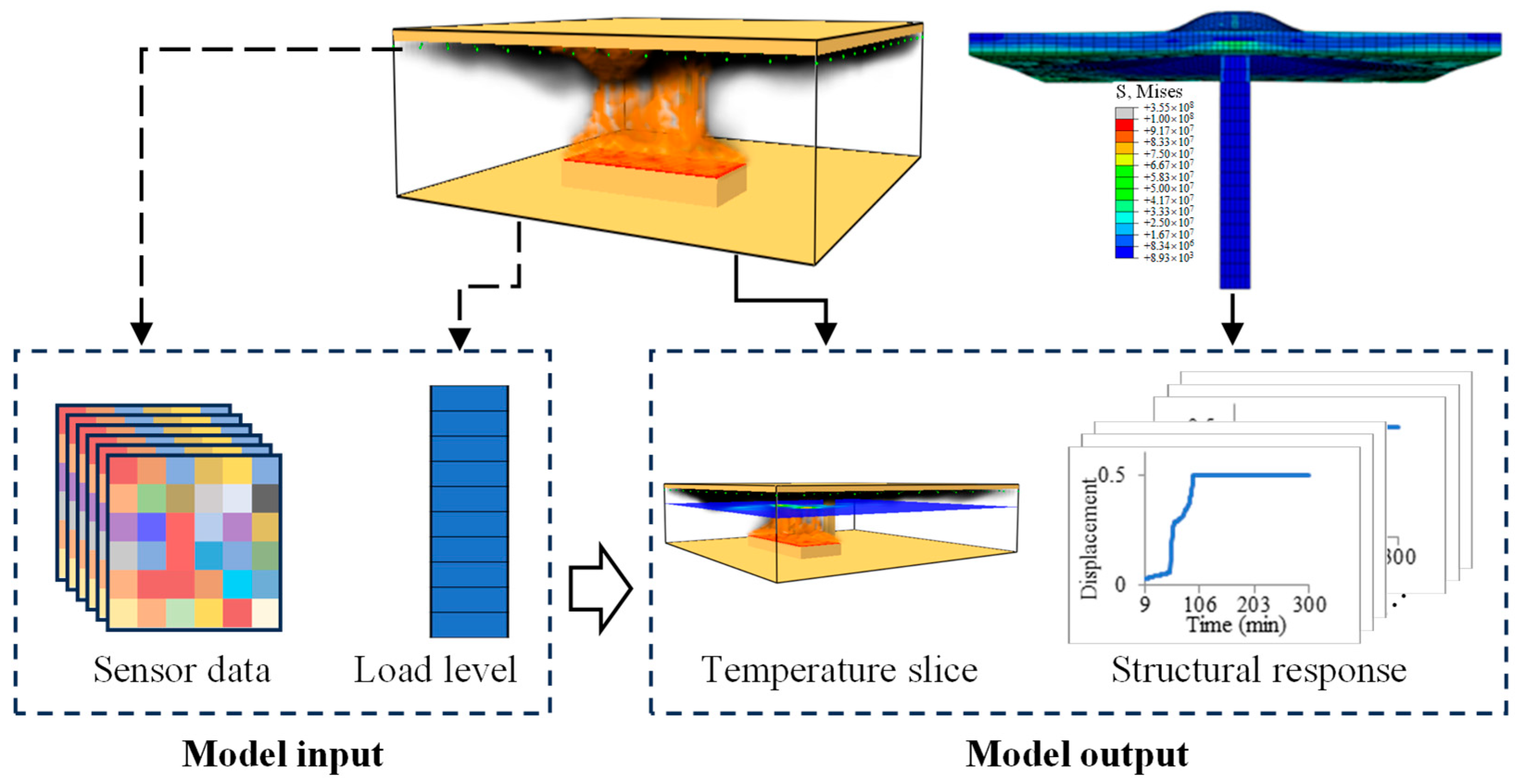
The combination of (a) and (b) was regarded as the input of the proposed prediction model, as illustrated in Figure 6. (c) and (d) were the expected outputs of Branch I and II, respectively. The 10 s sequence of sensor temperature and load level, the gas temperature distribution and deflection at a certain moment formed a training sample. Therefore, for the 27 structural fire scenarios, with 292 samples in each scenario, a total of 7884 training samples were produced. All the training samples were shuffled and divided into training and testing datasets in an 8:2 ratio.

The mean squared error (MSE) defined as the mean of the squared differences between predicted and expected results was selected as the loss function for both the prediction of temperature distribution and deflection.

$${MSE}_j={\displaystyle \frac{1}{n}}{\sum }_i{\left(y_i-{\widehat{y}}_i\right)}^2,$$

(1)

where i is the ith training sample, n is the number of samples, $y_i$ is the actual value of the ith sample, ${\widehat{y}}_i$ is the predicted value of ith sample, j is the label of Branch I or II. A simple combination of the loss functions ${MSE}_{total}$ was formed and chosen as the final loss function of the proposed model since the two branches were trained simultaneously.

$${MSE}_{total}={MSE}_I+{MSE}_{II},$$

(2)

The coefficient of determination R² was selected as the metric to measure the performance of the model in fitting data, and how well it can predict the outcomes.

$$R^2={\displaystyle \frac{\sum _i{\left({\widehat{y}}_i-\overline{y}\right)}^2}{\sum _i{\left(y_i-\overline{y}\right)}^2}},$$

(3)

where $\overline{y}$ is the average value. The value of R² is in the range of 0 and 1. The model explains a large proportion of the variability in the data if a high R² value is attained, and a value of 1 indicates that the model perfectly fits the data. Pytorch 3.8 was adopted to build the proposed deep learning model in this study. The model was trained for 200 epochs on a server with a GeForce RTX 4080 graphics card and 32 GB of physical memory, lasting about 2 h. The value of Branch I and II, as well as the overall value of loss and R² evolving with training epochs, were obtained.

4. Results and Discussion

4.1. Validation of Modelling Approach

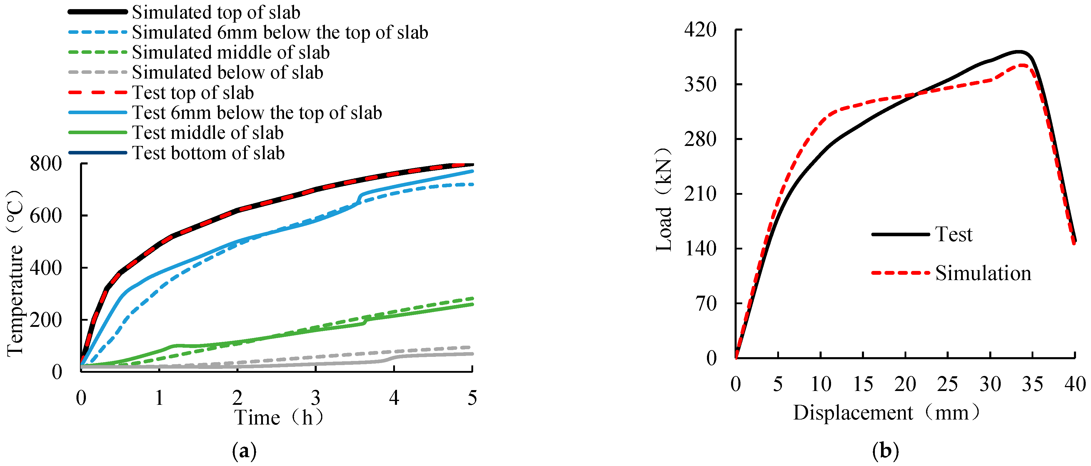
The FE model of the flat slab–column joint was validated with previous fire tests before it was applied to simulate the thermomechanical responses. During the tests [8,53], the central area of the bottom surface of the tested slab was exposed to high temperature generated by ceramic fibre heating panels. The temperature at the locations of the top slab surface, 6 mm below the top surface and the bottom surface was measured by thermocouples. FE models with geometries, material properties and loading conditions being the same as those of the tested specimen were established in Abaqus. The concrete temperatures at the locations same as those in the tested specimen were obtained. As illustrated in Figure 7a, the simulated temperature variations were closely aligned with the experimental results, demonstrating the feasibility of the modelling approach in capturing the thermal response of a flat slab–column joint under fire.

The column was pulled up with an upward-moving arm while keeping the edges of the slab clamped. The loading evolving with the applied deflection was then obtained and compared with the test results, as presented in Figure 7b. The loading experienced an initial linear increase stage, a slow growth stage and a final linear decrease stage, which coincide with the curve from the test results. The simulated maximum load-bearing capacity of the joint was 365 kN, which was only 4% lower than the test results of 380 kN. The coincidence between the simulated and tested results demonstrates the accuracy of the established model in capturing the structural response of the flat slab–column joint at ambient temperature.

4.2. Verification of the Model Hyper-Parameters

A sensitivity analysis was conducted on the hyper-parameters of the proposed deep learning algorithm, including learning rate, optimizer, and the spatial and temporal intervals of the input data. As illustrated in

Table 1. The sensitivity analysis on the hyper-parameters of the proposed model.

Values of Hyper-Parameters	R2 of Branch I (%)	R2 of Branch II (%)
Learning rate: 0.0001	92	93
Learning rate: 0.01	88	86
Optimizer: SDG	90	55
Optimizer: AdaGrad	91	91
Sensor interval: 2 m	91	93
Sensor interval: 3 m	91	90
Input temperature duration: 5 s	91	87
Input temperature duration: 8 s	91	91
Adopted model (learning rate: 0.001, optimizer: Adam, sensor interval1 m, input temperature duration: 10 s)	92	95

, the influence of the hyper-parameters on the R² values was complicated. A higher learning rate may accelerate the convergence, but the trained model may not perform well. The model with a learning rate of 0.01 could only attain values lower than 90%. The verification on the commonly used optimizers of SDG, AdaGrad, and Adam indicated that Adam attained the highest value of R², while the model trained with the optimizer SDG attained an extremely low value of 55% on Branch II. The sensitivity analysis on the spatial and temporal intervals of the input was then conducted after determining the learning rate and optimizer. The value of R² increased with the decrease in the sensor distance and sensor collection interval, which conforms to intuitive cognition, as more information was given as the input data to the model.

The optimised hyper-parameters of learning rate, optimizer, sensor spatial interval, and temporal intervals were 0.001, Adam, 1 m, and 1 s, respectively. The model with these optimised hyper-parameters was then used for the prediction of the temperature distribution and deflection. It should be mentioned that though the model with these hyper-parameters may perform well on the datasets considered in the current study, it does not mean the model will have similar performance in practice. The datasets were constructed with numerical simulations rather than real fire scenarios, which may be different and much more complicated than the scenario considered in the current study. In addition, the performance of the model can be further enhanced by conducting a thorough sensitivity analysis of the hyper-parameters. However, the model constructed in this study could be a meaningful attempt to predict fire and structural responses and to give an alarm fusing the fire emergencies and structural collapse. The training datasets and the trained model are provided in the Supplementary Materials to facilitate validation and further studies.

4.3. Prediction of Temperature Distributions

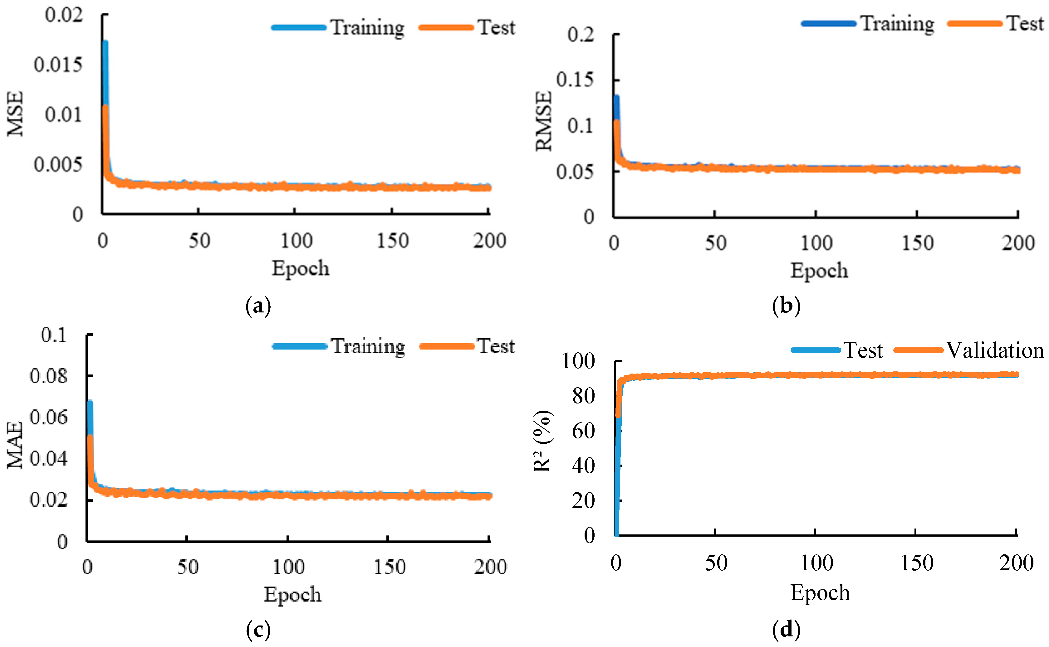
Branch I of the proposed model was used to predict the temperature distribution at a height of 2 m above the ground. Figure 8 presents the variations in MSE, RMSE, MAE, and R². During the initial phase of training, the value of MSE, RMSE, and MAE decreased rapidly and eventually converged to 0.003, 0.05, and 0.02, respectively. The R² value increased progressively throughout the training process and ultimately reached 92%. The close overlap between the training and test curves indicates that the model performs well on both. These training results convincingly validate the feasibility of the proposed algorithm for predicting the spatial temperature distribution 3 min in advance under the described parking garage fire scenario.

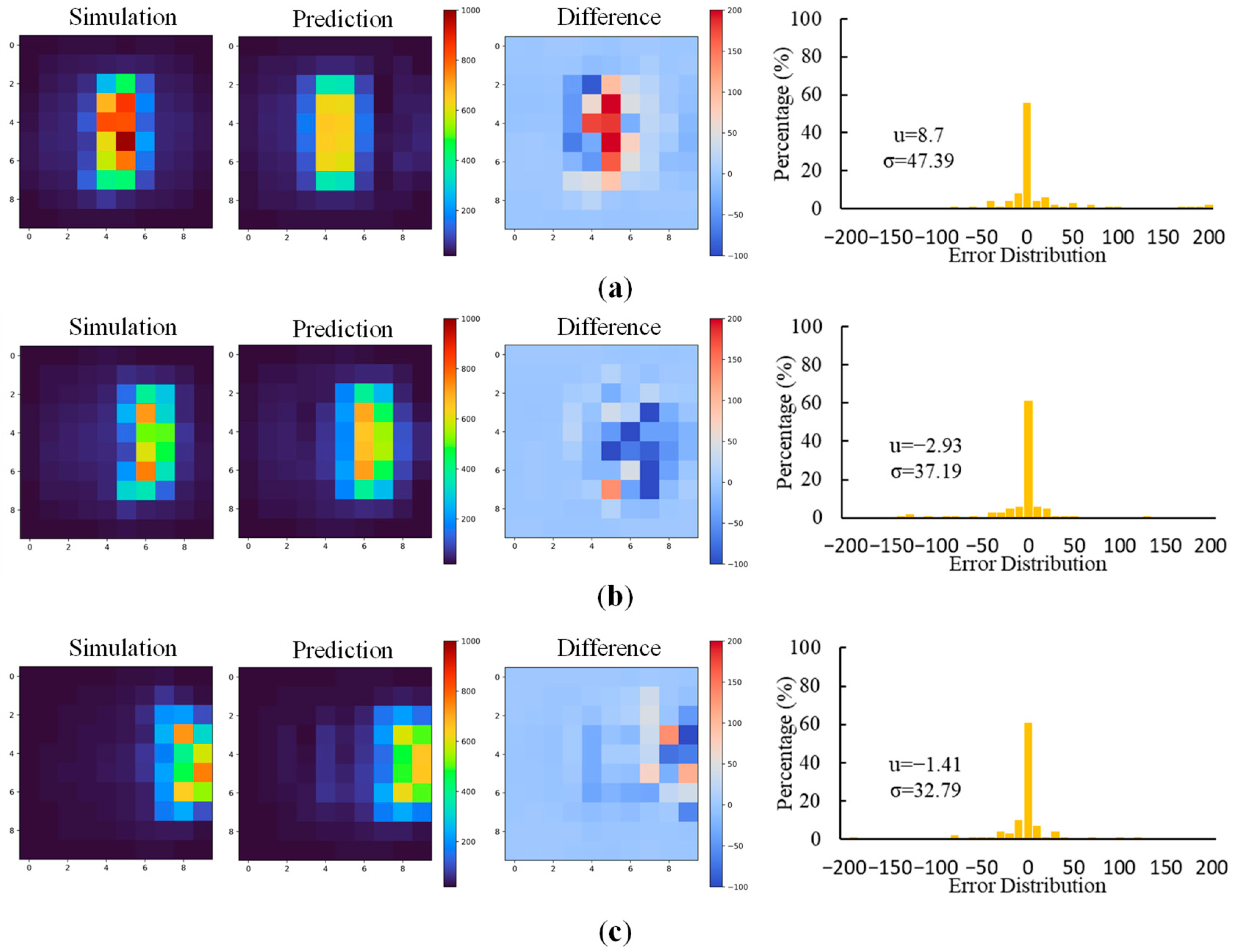
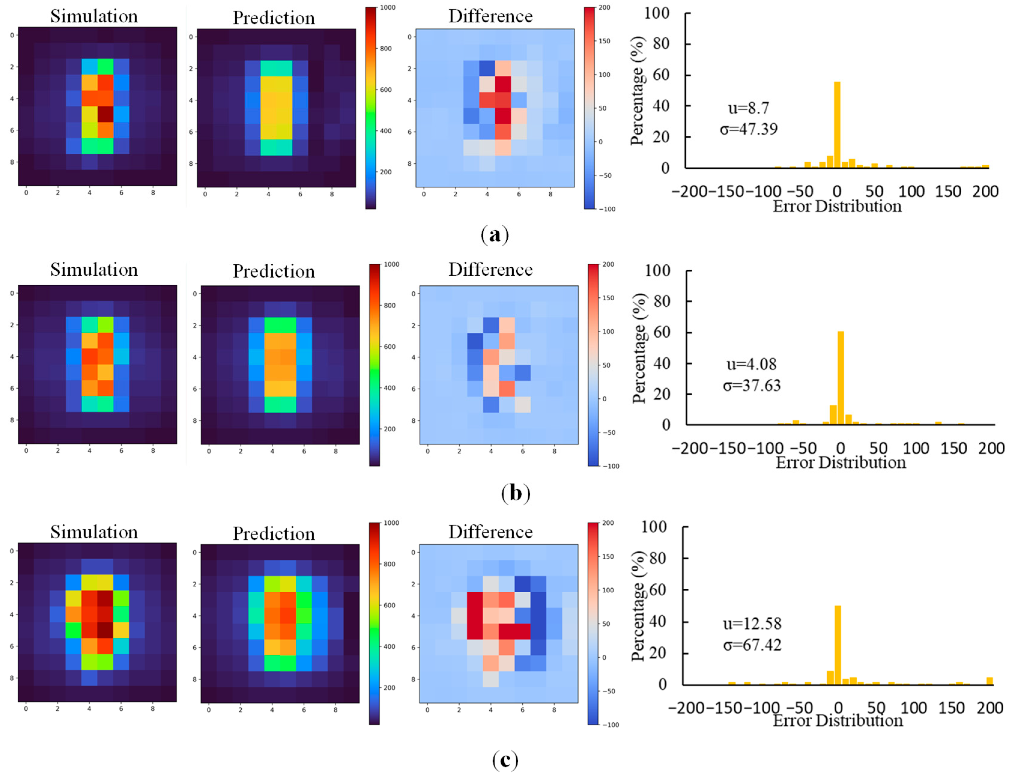
To verify the specific performance of Branch I of the model in predicting temperature distribution, the predicted results and the corresponding simulation results were compared in Figure 9 and Figure 10. The subfigures from left to right were the simulated and predicted temperature distribution, the spatial variation in the temperature difference, and the statistical error distribution calculated with the temperature difference. The predicted and simulated temperature distributions coincided with each other. The average value and the standard deviation of the difference between the predicted and simulated distribution were roughly within 10 °C and 50 °C, respectively, which could be an acceptable deviation for practical firefighting. The location of the fire source can be easily identified from the predicted results shown in Figure 9, since the higher temperature area moves with the location of the fire source. The severity of the fire could also be roughly estimated from Figure 10 since the area with higher temperatures expanded with the value of HRR. Though there are slight discrepancies between the predicted and actual temperature distributions, their overall coincidence confirms the effectiveness of the model in predicting the spatial temperature distribution at a height of 2 m in car park fire scenarios.

4.4. Prediction of Structural Responses Under Fire

Branch II of the proposed model was used to predict the vertical deflection at the edge of the slab, which would experience the largest deflection under fire. Figure 11 presents the variation curves of MSE, RMSE, MAE, and R² with respect to training epochs. In the early stage of training, MSE, RMSE, and MAE decreased rapidly, then continued to decline, converging to 0.003, 0.05, and 0.03, respectively. The R² value increased steadily until it reached 95%. Owing to the adoption of a dropout rate of 0.2 during training, the test curves were slightly higher than the training curves. This regularisation technique compelled the network to learn more robust features with reduced interneuron dependence and higher generalisation capability, while all neurons were activated during testing. The close overlap between the training and test curves indicates that no overfitting occurred. The R² value as high as 95% strongly demonstrated the feasibility and superior performance of the proposed algorithm in predicting structural deflection within the first 300 min of a parking garage fire.

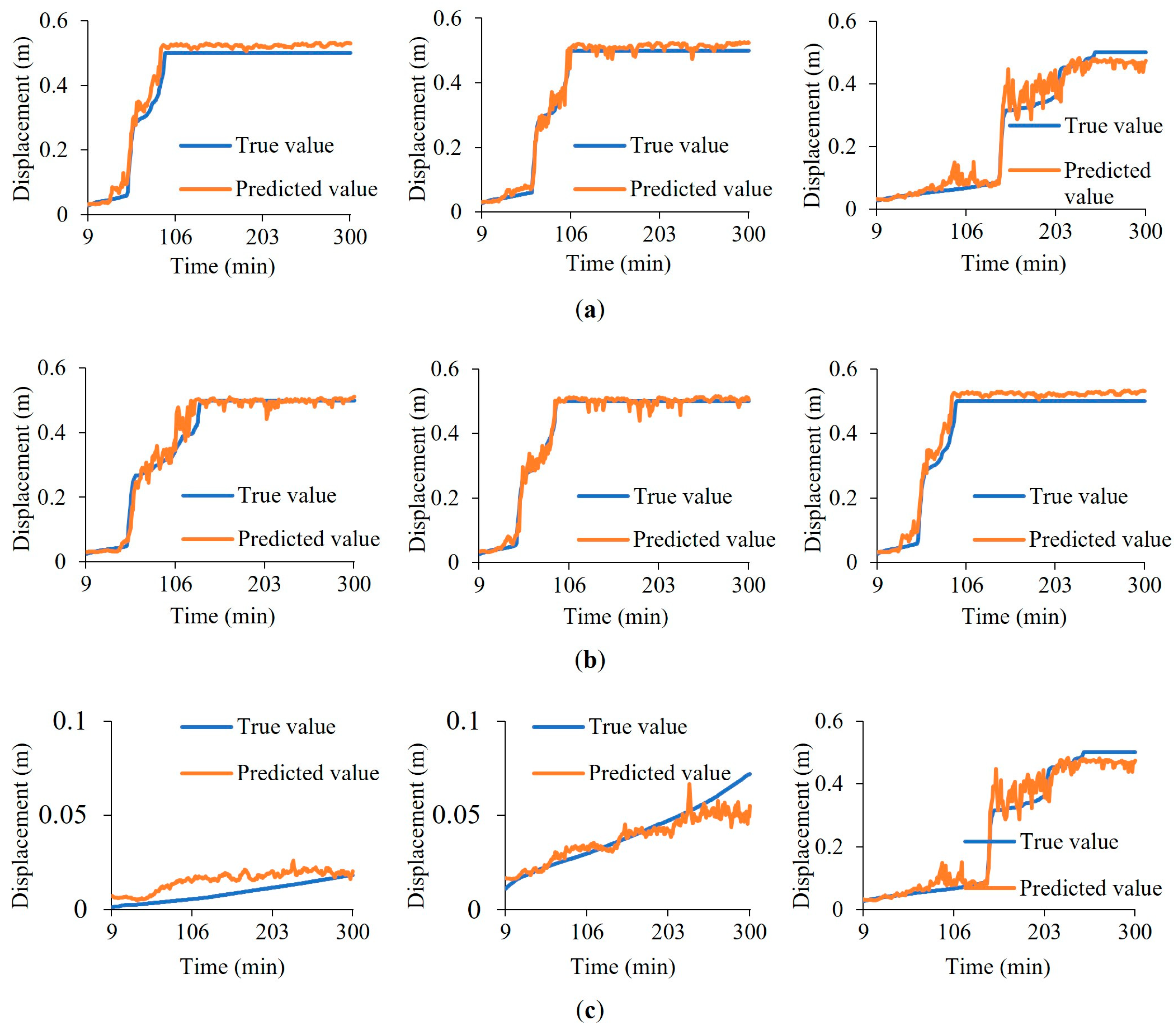
Figure 12 compares the prediction of the slab deflection of the model under various scenarios. As illustrated, the predicted deflection curves closely align with the simulations, indicating the high capability of the model in giving a prediction of the mechanical responses of a car park on fire, considering the effects of fire source location, fire size, and the applied load level. This could be attributed to the established model that has learned the mapping between the input and output after training. Additionally, good performance may also indicate that predicting the trend of the deflection curve is a relatively easy task for a deep learning model with many weights.

The simulation results show the evolution of the slab deflection experienced four stages, including a slow linear increasing stage, a sudden increasing stage, a nonlinear increasing stage, and a constant stage, where the structure collapses. The structures collapsed in a fire because the slab edge reached the deflection limit of 0.49 m rather than the rate of deflection 21.8 mm/min. The model performs well at the initial slow linear increasing stage, which may be due to the gentle, slow trend being easier to learn. The performance of the model at the nonlinear increasing stage and the constant stage was relatively unsatisfactory, with slight fluctuations.

A further detailed comparison was conducted to check the performance of the model during the whole fire exposure. The simulation results show that the evolution of the slab deflection experienced four stages, including a slow linear increasing stage, a sudden increasing stage, a nonlinear increasing stage, and a constant stage, where the structure was regarded as collapsed after attaining the maximum constant value of 0.49 m. 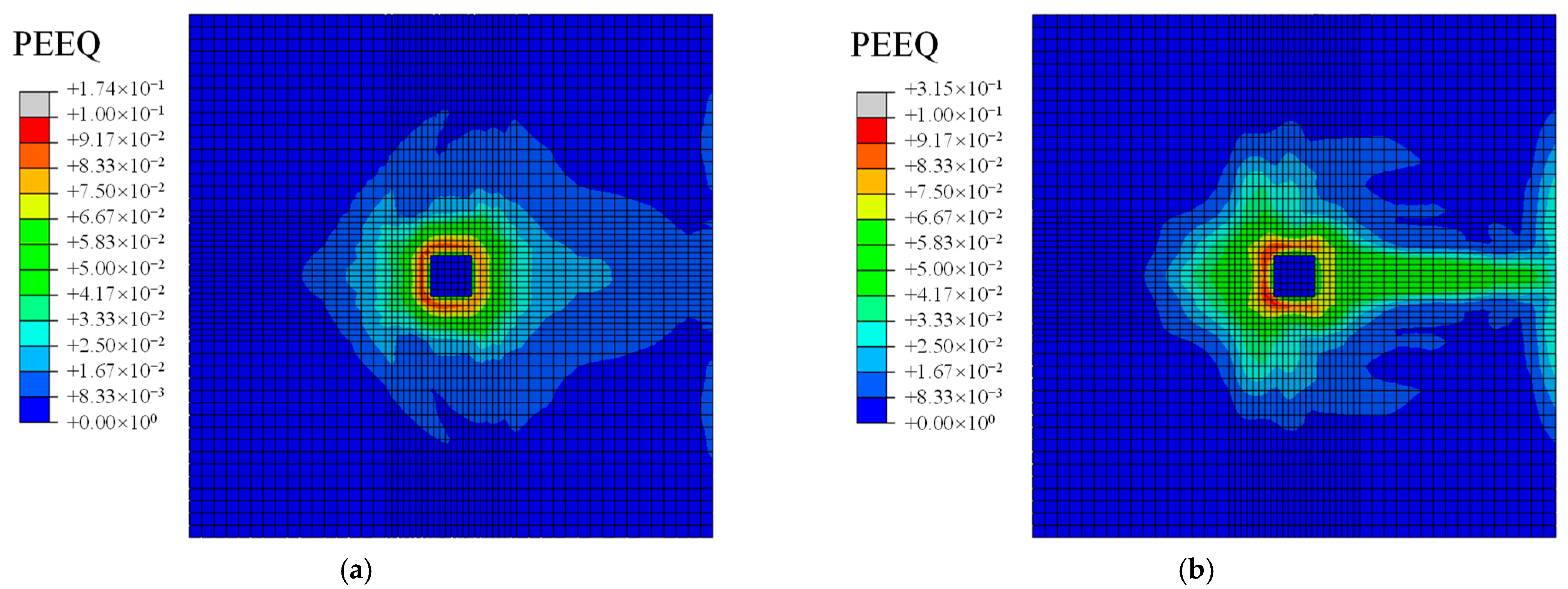As illustrated in Figure 12, the prediction was less accurate in the period of 65 min to 200 min, where the predicted results exhibit an upward trend. The finite element modelling (Figure 13) reveals that the cracks in the concrete slab gradually expanded from the location of the column to the slab edges, leading to a reduction in structural load-carrying capacity and a gradual increase in deflection. The proposed network failed to fully capture this characteristic. Similarly, a noticeable discrepancy between the predicted and actual deflections when the structure failed was observed, as shown in Figure 12c. The concrete at the slab–column joint area suddenly failed at around 140 min. The equivalent plastic strain pattern of the structure near the conjunction area shows that the cracks extending from the slab–column conjunction to the slab underwent a complete development and formation process within a relatively short time period, inducing a significant deflection at the slab edges as illustrated in Figure 13b. The proposed algorithm, however, cannot fully capture the process of crack initiation and sudden penetration in flat plate–column connections under fire conditions. This limitation leads to a slightly larger deviation between the predicted and simulated results. Nevertheless, the predictions are still within an acceptable range.

It should be mentioned that, initially, the deflection rate was also selected as an output of the model, but the predicted deflection rate fluctuated significantly, making it challenging to figure out the time when the deflection rate reaches the criteria. Thus, the deflection rate was not included as a model output. In addition, the time to collapse could be directly used as a model output. However, more valuable information about the structural response can be obtained by using deflection evolution over time as the output. The time to collapse can be readily obtained from the predicted deflection evolution through a simple post-processing calculation. In addition, the model would not necessarily be retrained if the collapse criteria changed. Optionally, both the deflection and the time to collapse could be used as outputs. However, the latter was not selected as an output in this study as it would duplicate information, given that we already have the deflection evolution.

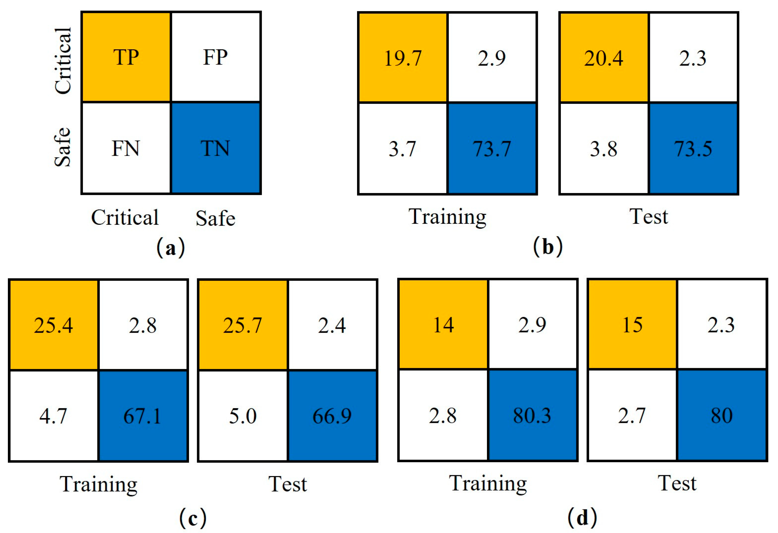
For structural safety, a large deflection, which is 0.49 m in the current study, indicates the collapse of the structure under fire. In terms of fire safety, previous studies [46] indicate that inhaling air temperatures exceeding 60 °C can cause mild burns to the respiratory tract, and if temperatures in areas below 2 m height exceed 60 °C, humans will find it intolerable. This value is adopted in the study as the safety limit. Most of the current studies focus on fire safety, ignoring the potential occurrence of structural collapse. In this study, both fire and structural safety were considered. Reaching an average value of the temperature distribution of 60 °C or an edge deflection limit of 0.49 m was classified as a dangerous state. The predicted results were calculated and classified into two states: safe or critical (dangerous). The confusion matrix was used to assess the model’s prediction performance. The values of true positive (TP), false positive (FP), false negative (FN), and true negative (TN) were calculated. Ideally, the data should be fully distributed along the diagonal, indicating a perfect match between the true and predicted values. As illustrated in Figure 14b, most of the predicted results coincide with the actual values, with only 6% of the predicted results distributed outside of the main diagonal cells. The detailed classifications considering fire safety or structural safety were presented in Figure 14c and Figure 14d, respectively. The vast majority of the data was distributed along the main diagonal, indicating the good performance of the model in predicting the critical event in the aspect of fire or structural safety. It also performs well. The results show that the proposed model can give commendable predictions on potential critical events where fire or structural collapse may threaten the lives of firefighters and trapped personnel.

4.5. Prediction of Responses in Unseen Fire Scenarios

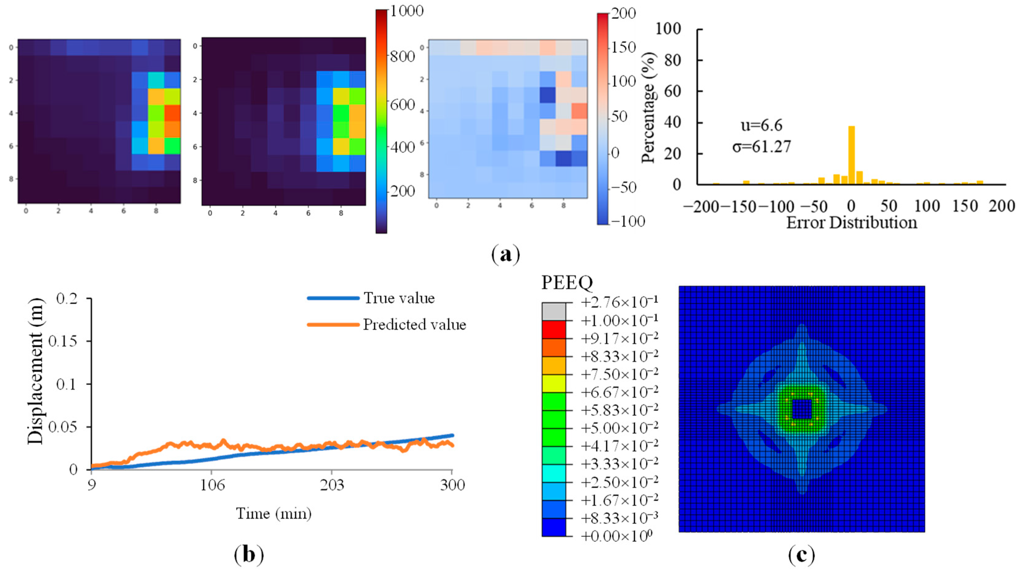
In the current study, a representative single slab–column joint area was selected to establish and validate the method framework, but the relatively simple structure has certain limitations. The boundary or ventilation conditions, which are common in real car parks, are challenging to model accurately for the partial structure. Good ventilation conditions were assumed, with the four sides of the assumed space set as open boundary conditions, allowing the smoke generated by the fire to diffuse freely in all directions. However, the tuned model trained with open boundary conditions demonstrated its potential in the unseen scenario. A new fire scenario in which one side was blocked by a wall, mimicking the case where a column was near the side of the whole structure, was modelled. The trained model was used to predict the structure’s thermal and mechanical responses. As illustrated in Figure 15, the average and standard deviation of the difference between the expected and simulated distributions were within 6.6 °C and 61.27 °C, respectively, which were comparable to those of the trained scenarios. The predicted deflections also closely align with the simulations. However, it should be acknowledged that a thorough analysis of the influence of boundary conditions and ventilation is required before the method is applied in practical firefighting.

Though the proposed model performs well in predicting the thermal and structural responses and the critical events, the approach has certain limitations. The training data were generated from numerical simulations, which may not capture all the complexities of real-world fire scenarios, including complex ventilation conditions and fire spread dynamics. In addition, over the past few years, electric vehicles have become increasingly widespread. Electric vehicles pose higher combustion risks, and it is difficult to extinguish them; their batteries also pose an additional risk of explosion at any time during combustion. Future research could further investigate the dynamic development of electric vehicle fires and the more severe impacts of explosions on structures. The structural model, though representative, is a simplified substructure. Furthermore, the deep learning model, while effective, exhibited slight deviations in predicting highly nonlinear structural behaviour, such as the rapid deflection increase during concrete cracking and at the point of failure, indicating that capturing the intricate failure mechanism remains challenging and the capability could be further improved with more layers and training data. Future work should focus on validating the framework with data from large-scale fire tests and real fire incidents to enhance its robustness. The model could be extended to incorporate more complex car park geometries, multiple fire sources, and the activation of fire protection systems. Exploring more sophisticated network architectures to explicitly model the structural topology may further improve prediction accuracy, especially for complex failure modes.

5. Conclusions

This study developed a deep learning framework for the real-time prediction of thermal and structural responses in reinforced concrete car park fires by leveraging the pattern recognition capabilities of deep learning. A comprehensive numerical database was constructed through systematic simulations with FDS and Abaqus, accounting for key influencing factors including fire source heat release rate, fire location relative to a critical column, and the applied load on the slab. A hybrid CNN-LSTM model was designed to process temporal sequences of sensor data. The model utilises historical data from temperature sensors along with the structural load level, to make predictions simultaneously, the future spatial temperature distribution at a height of 2 m and the time-dependent deflection at the edge of the slab. Results demonstrate the model’s high predictive capability, with coefficients of determination R² reaching 92% for temperature distribution 3 min ahead, indicating that the firefighters could have 3 min for preparation before the predicted scenario occurs. In addition, the model achieved 95% for R² value in predicting structural deflection over a 5 h period so that the firefighters could have a general idea how the structure would behave in the following 5 h after fire starts. The model’s performance was further checked by its ability to accurately classify critical safety states based on predefined thresholds. The confusion matrix analysis confirmed a high rate of correct classification, with only 6% of overall predictions being erroneous, underscoring the model’s reliability for early warning. The deviations are within acceptable limits for practical firefighting applications.