Article

Density-Based Spatial Clustering of Vegetation Fire Points Based on Genetic Optimization of Threshold Values

by
Xuan Gao
1,2,
Tao Wang
1,2,* and
Ke Xie
1,2
1
College of Resource Environment and Tourism, Capital Normal University, Beijing 100048, China
2
Key Laboratory of the Ministry of Education Land Subsidence Mechanism and Prevention, Capital Normal University, Beijing 100048, China
*
Author to whom correspondence should be addressed.
Fire 2025, 8(11), 431; https://doi.org/10.3390/fire8110431 (registering DOI)
Submission received: 8 September 2025 / Revised: 27 October 2025 / Accepted: 30 October 2025 / Published: 31 October 2025

Abstract

Vegetation fires are among the most common natural disasters, posing significant threats to people and the natural environment worldwide. Density-based clustering methods can be used to identify geospatial clustering patterns of fire points. It further helps reveal the spatial distribution characteristics of wildfires, which are crucial for regional-specific fire mapping, prediction, mitigation, and protection. DBSCAN (density-based spatial clustering of applications with noise) is widely used for clustering spatial objects. It needs two user-determined threshold values: the local radius and the minimum number of neighboring points for core points, which require user expertise and background information. This work proposes a dual-population genetic optimization to determine threshold values of DBSCAN for clustering vegetation fire points in western China. By constructing randomly generated threshold populations, optimized threshold values are obtained through crossover, mutation, and inter-population exchange, measured by multiple clustering metrics. Focusing on vegetation wildfires in western China during 2016–2022, the results reveal that vegetation wildfires can be divided into eight regions, each exhibiting distinct spatiotemporal patterns and geographic contexts.

1. Introduction

Vegetation fires are one of the most common types of wildfires. In recent years, the frequency and intensity of vegetation fires have increased significantly under the combined influence of anthropogenic activities and climate change [1]. Between 1979 and 2013, the globally burnable area doubled, and the average fire season length increased by 18.7% [2]. In August 2021 alone, over 28,000 fires occurred in the Amazon rainforest, exceeding the historical average for three consecutive years and causing severe forest degradation [3]. And between 2001 and 2023, the affected area and tree cover loss have been increasing significantly [4]. Forest and grassland fires significantly impact global ecosystems and economies. The vegetation fires release substantial amounts of water vapor, carbon dioxide, methane, and aerosol particles into the atmosphere, altering the Earth’s radiation balance and further exacerbating climate change [5]. Between 1997 and 2016, global carbon emissions from wildfires amounted to approximately 2.0 PgC/a (1 Pg = 1015 g), which has accelerated global warming [6]. Moreover, vegetation fires pose severe threats to economic stability and human safety. Between 1999 and 2018, approximately 100,000 forest fires occurred in China, destroying vast areas of forest and agricultural land, with total economic losses exceeding 2 billion RMB [7].
Understanding spatio-temporal patterns of vegetation fires can help the public and private sectors take appropriate measures and prepare for fire disasters. Various methods have been employed to analyze and understand fire patterns. Statistical methods can analyze historical fire data, such as fire frequency and burned area. Yi et al. analyzed wildfire data in China from 1950 to 2010, concluding that spring and autumn are peak wildfire seasons, with most fires occurring in northeastern and southwestern provinces [8]. Donovan et al. analyzed large wildfires (burned area larger than 200 hectares) in the United States (US) from 1984 to 2020, finding an upward trend in wildfire scale, frequency, and burned area in southern and eastern regions [9]. Spatial analysis, as a special type of statistical-based method, focuses on the geographical distribution and regional patterns of vegetation fire occurrences. Spatial analysis methods can further assist firefighting departments in adopting region-specific measures and help the general public prepare to mitigate wildfire threats. Hot spot analysis is a spatial statistics method that aims to pinpoint areas where data values cluster in a statistically significant manner, thereby discerning regions of elevated (hot spots) or diminished (cold spots) activity. Reddy et al. used hotspot analysis to investigate forest fires in South Asia, identifying concentrated fire activity between January and May, particularly in Bangladesh [10]. Sperry et al. applied hotspot analysis to wildfire data in South Carolina (US), finding higher fire frequency in the southern part of the state [11]. Prasertsri et al. used geographically weighted regression (GWR) to analyze the relationship between elevation, slope, surface temperature, and wildfire incidence, and further developed a wildfire risk model for Thailand’s Tadesong Forest Park, with an R-squared value exceeding 82% [12,13]. Cong et al. combined geographically weighted Gaussian regression (GWGR) and optimized hotspot analysis (OHSA) to study wildfire patterns in the Amazon, revealing concentrated fire activity in northern Rondônia and southern Amazonas [14]. Singh et al. developed a hybrid model using support vector machines and random forests for wildfire prediction, achieving 94% accuracy with data from Indian forests during 2011–2020 [15]. In recent years, artificial intelligence methods have been gradually introduced to enhance insights and predictive capabilities regarding fire patterns [16].
Spatial clustering [17,18] is a key tool in spatial analysis, and relevant methods are widely used to understand the spatial heterogeneity of wildfires in different clusters. Tian et al. used Ripley’s K spatial clustering method [19] to analyze vegetation fire distribution in northern China, identifying significant clustering in Heilongjiang, Jilin, Liaoning, and Hebei provinces [20]. Baykal conducted a comprehensive performance assessment of three spatial clustering and autocorrelation methods in forest fires based on a number of indicators [21]. Khairani et al. investigated fire-prone areas from Indonesia using the K-Means method to classify regions into high hotspot occurrence areas, non-hotspot high occurrence areas, and areas prone to frequent fire hotspots [22]. However, K-means algorithms can only identify convex clusters and can hardly accommodate multiple shape variance clusters intertwined, which are common in applications. And it is not designed to detect outliers that do not belong to any clusters. DBSCAN, Density-Based Spatial Clustering of Applications with Noise, is a widely used clustering approach that identifies clusters based on the spatial density of objects [23]. In general, researchers have been looking for more computationally efficient implementations of DBSCAN, especially in big data applications, by introducing index structures and accommodating approximation of clustering results [24]. Ahajjam et al. employed DBSCAN to conduct spatio-temporal clustering of wildfire events in Alaska, the U.S. [25]. The clustering results were then used for calculating the area of burnt regions and making various wildfire occurrence prediction tasks based on machine learning.
DBSCAN can handle clusters of arbitrary shapes and detect noise points from clusters. It needs two threshold values. One is a neighborhood radius (Eps), which is used to indicate spatial density. Another is the minimum number of neighboring points within a core point (MinPts), which is used to filter out those noise points or outliers. These two values significantly influence the clustering results. And their selection often relies on users’ expertise and understanding of the research phenomena. Currently, threshold optimization methods mainly include Genetic Algorithm (GA), Simulated Annealing (SA), and Particle Swarm Optimization (PSO). In this field of research, the GA has demonstrated excellent performance [26]; hence, it is selected as the threshold optimization method. Gebril et al. proposed a hybrid approach to automatically determine the optimal value for each Eps value that incorporates the Genetic Algorithm (GA) with the DBSCAN algorithm [27]. However, how to determine both threshold values in one solution remains a question.
This study proposes a dual-population genetic algorithm to select the two threshold values in DBSCAN. Using vegetation fire data from western China during 2016–2022, the study compares clustering results with different threshold selections using multiple clustering performance indicators. An additional synthetic test dataset is used to validate the performance of the proposed approach. To validate the effectiveness of the proposed method, the clustering results were evaluated using the Silhouette Index, Calinski–Harabasz Index, Davies–Bouldin Index, and SD Validity Index. The results show that the dual-population genetic algorithm effectively identifies optimal threshold values for DBSCAN. Based on the resulting vegetation fire clustering results, we further analyze the spatiotemporal distribution patterns of vegetation fires in the study area.

2. Materials

2.1. Study Area

In recent years, the forest area in China has increased from ∼154 Mha in 2000 to ∼248 Mha in 2022, in which the western regions of China dominate the increasing forest area [28]. Vegetation fires are frequent in western China due to various causes. This study region includes the provinces of Inner Mongolia, Guangxi, Chongqing, Sichuan, Guizhou, Yunnan, Tibet, Shaanxi, Gansu, Qinghai, Ningxia, and Xinjiang, which cover an area of 6.867 million km2 and account for 71.5% of China’s total land area (Figure 1). In government administration, Inner Mongolia is taken as a part of West China, although geographically, the eastern part of this province is considered part of Northeast China. Regions such as Yunnan and Guizhou, with dense forests and intensive anthropogenic activities, experience high incidences of human-caused fires [29]. In Inner Mongolia, lightning-induced fires are prevalent and have increased in recent years [30]. Qinghai and other inland regions with scarce precipitation are prone to vegetation fires during dry seasons [31]. Spatial clustering analysis can facilitate the identification of vegetation fires which share similar causing factors. The clustering results can support the formulation of targeted preventive strategies to mitigate economic and ecological risks.

2.2. Research Data

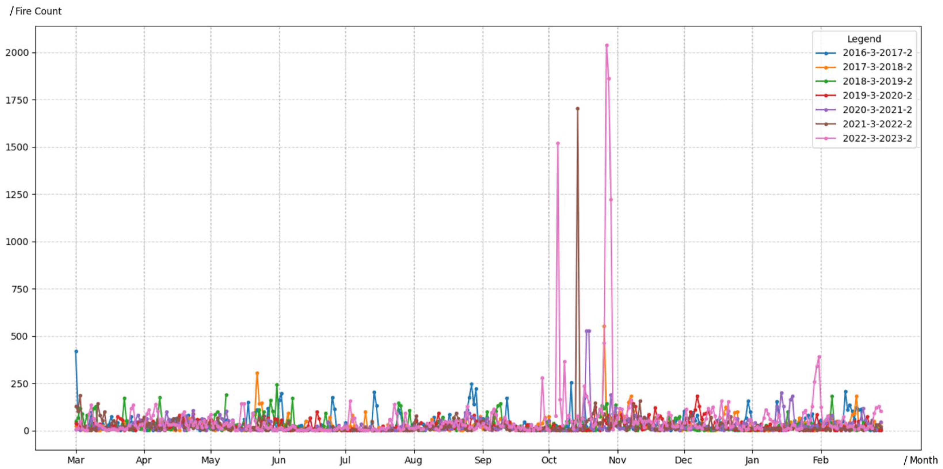
This study uses vegetation fire data from Himawari-8, a satellite launched by Japan in July 2015. Compared to other fire data acquired by remote sensing satellites, such as MODIS and Sentinel 3, Himawari-8 offers higher temporal resolution up to 10 min, which can detect vegetation fires lasting a shorter time [32,33,34]. The dataset includes fire points with attributes such as time, geographic coordinates, fire point level, and confidence level. Fire point levels are classified as Level 1 (cooling), Level 2 (smoldering), and Level 3 (burning). Confidence levels are categorized as Level 1, Level 3, and Level 5, determined by factors such as solar radiation and brightness temperature. This study uses fire Level 3 (burning) and confidence Level 5 (highest confidence) [33,34] to filter fire points from 2016 to 2022, resulting in 84,330 fire points. There are 28,381 fire spots with non-repeating longitude and latitude coordinates. Figure 1 shows the study region and spatial distribution of fire points. Figure 2 presents daily fire point statistics, which show high fire incidence in the fall.
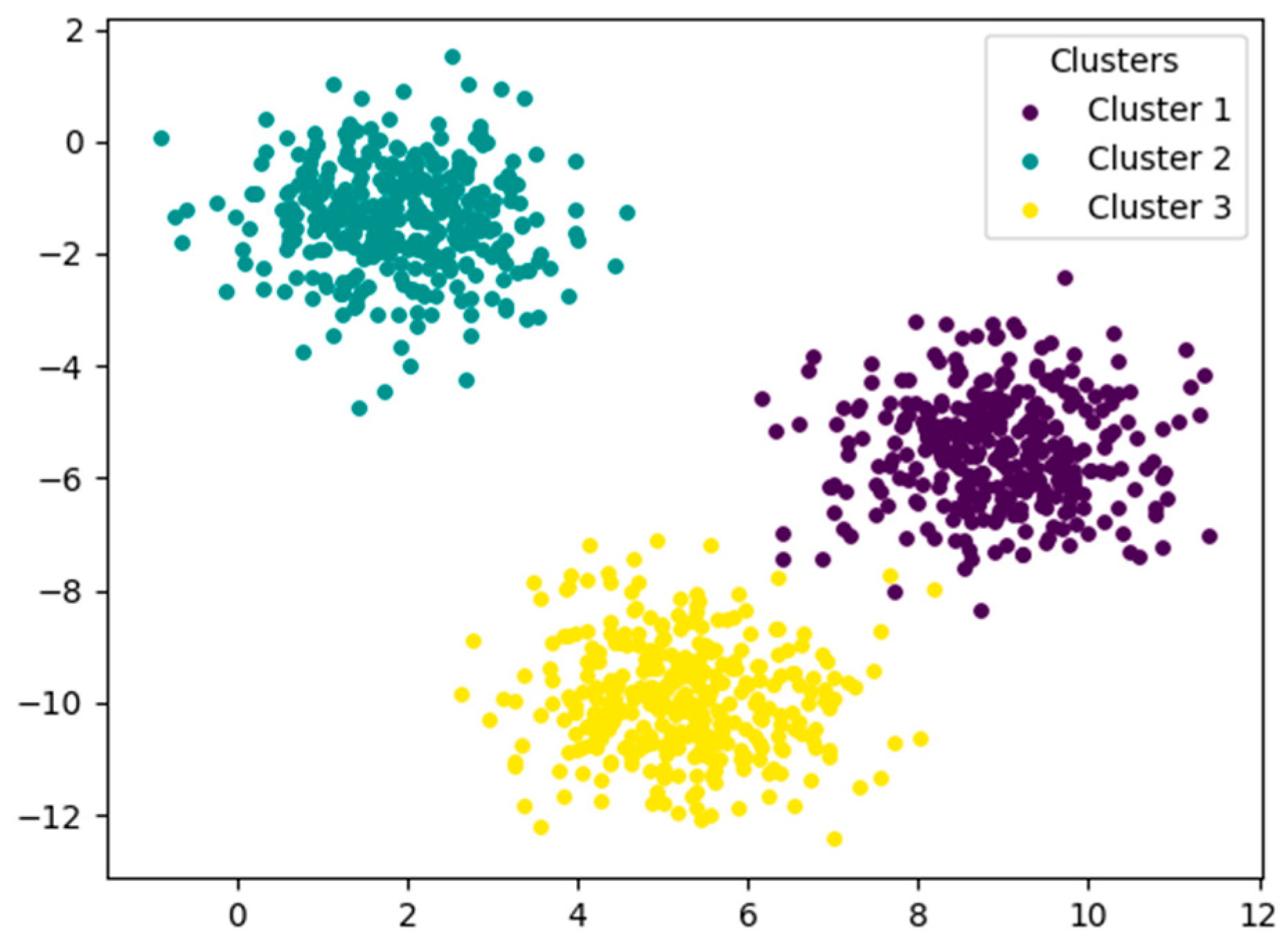
To validate the proposed DBSCAN with GA optimized threshold values, A synthetic test dataset following a Gaussian distribution was generated, comprising 1000 sample points forming three distinct clusters with an intra-cluster standard deviation of 1.0 (Figure 3). The dataset was constructed using the make_blobs function, a core dataset generation utility within the scikit-learn library [35]. This tool is specifically designed to produce synthetic datasets consisting of one or more “blobs”, where data points in each blob adhere to a simple probability distribution—namely, the multivariate Gaussian distribution here. The mathematical foundation of make_blobs relies on the multivariate Gaussian distribution. For a blob k (with k = 3 in this study) in a d-dimensional feature space (where the number of features corresponds to the dimensionality; for consistency with coordinate representation, this study uses d = 2, i.e., two-dimensional data), the data generation process is formally defined as follows:
Let the center of the k-th blob be denoted by the vector μ_kR^d, and its covariance matrix Σ_k be constrained to an isotropic form, i.e.,
Σ _ k = σ _ k ^ 2 I
where σ_k is the standard deviation of the k-th blob (specified by the parameter cluster_std; this study adopts the default value of 1.0), and I is the d × d identity matrix.
Under this isotropic assumption, each data point x_i^((k))∈R^d generated for blob k is obtained via:
x _ i ^ ( ( k ) ) = μ _ k + ε _ i
where each component ε_i^((j)) of the noise vector ε_iR^d is independently and identically sampled from a univariate Gaussian distribution with mean 0 and standard deviation σ_k:ε_i^((j))∼N(0, σ_k^2), for j = 1, 2, …, d.

3. Methods

Clustering is an unsupervised learning task designed to partition a dataset into multiple non-overlapping subsets, known as clusters. Each cluster represents a distinct group or category based on the user’s objectives. Normally, clustering algorithms group data points into clusters according to specific spatial distance, ensuring high intra-cluster similarity while minimizing inter-cluster similarity. This process enables the discovery of underlying patterns and structures within the data, supporting insightful analysis and actionable interpretations.

3.1. DBSCAN Clustering Method

DBSCAN is a density-based clustering algorithm that does not require prior specification of the number of resulting clusters. Instead, it groups data points based on spatial density distribution and can effectively identify noise within the dataset. The algorithm relies on two key threshold values: the neighborhood radius (Eps) and the minimum number of points within a neighborhood (MinPts). The neighborhood is a core concept in the algorithm, representing the range within which a sample point searches for other points to determine if they belong to the same cluster. Eps refers to the radius of a circular area centered around the sample point, within which other sample points are searched for. MinPts is the minimum number of sample points required to form a neighborhood [23].
Traditionally, selecting appropriate values for Eps and MinPts relies heavily on the user’s expertise and the user’s understanding of the data. To address this limitation, this study proposes a threshold selection method based on a dual-population genetic algorithm, enabling optimized parameter determination.

3.2. Dual-Population Genetic Algorithm for DBSCAN Optimization

Genetic algorithms are stochastic global search optimization techniques inspired by natural selection and genetic evolution [36,37]. These algorithms simulate biological processes, including replication, crossover, and mutation, to iteratively improve solutions to optimization problems. The process begins by encoding the optimization target into a computable string of codes, referred to as chromosomes, which collectively form an initial population. Each chromosome’s fitness is evaluated using a predefined fitness function, which quantifies its suitability relative to the problem’s objectives. Chromosomes with higher fitness scores are selected as parents and undergo crossover and mutation operations to produce offspring. These genetic operations introduce diversity and drive the population toward better regions of the search space. Through successive iterations, the population evolves, ultimately converging to an optimal or near-optimal solution. The multi-population Genetic Algorithm has been widely applied in recent years [38,39]. Accordingly, this study employs a dual-population Genetic Algorithm to optimize DBSCAN threshold values.
The main steps of optimizing DBSCAN threshold values using a dual-population genetic algorithm are as follows:
(1) Defining the estimated ranges for the thresholds Eps and MinPts, setting the population size, and specifying the maximum number of iterations. The ranges should be selected as wide as possible to ensure optimal performance. Two populations can be randomly initialized. Eps is encoded as a 64-bit binary number and MinPts as a 16-bit binary number. Zero-padding is applied if necessary. Each pair of Eps and MinPts values forms a chromosome within one of the populations.
(2) Performing DBSCAN clustering using the thresholds from all chromosomes in both populations. Referring to other research studies [40,41], the clustering results are evaluated using the silhouette index (S) as the fitness function (F), which measures the performance of each chromosome’s clustering results. The silhouette index quantifies the ratio of the distance between a sample point and its own cluster to the distance between the sample point and another nearest cluster. A higher silhouette index indicates better separation between clusters, reflecting superior clustering performance. The formulas for calculating S are as follows:
a x = 1 n i 1 y C i , y x d x , y
b x = m i n j , j i [ 1 n j y C j d x , y ]
F = S = 1 N C i 1 n i x C i b x a ( x ) m a x [ b x , a ( x ) ]
where Ci is the ith cluster, ni is the number of objects in Ci, NC is the number of clusters, and d(x, y) is the distance between x and y.
(3) Ranking all chromosomes in each population based on their fitness scores. The top 10% of chromosomes with the highest fitness are retained, and the remaining 90% for crossover with the best individuals are evaluated. The crossover probability is calculated as follows:
p = 1 F F s u m
where F is the fitness value and Fsum is the sum of fitness values.
If the crossover condition is met, each gene in the chromosome has a 50% chance of being replaced with the corresponding gene from the best individual. Both Eps and MinPts undergo crossover simultaneously.
(4) Retaining the top 50% of chromosomes based on fitness ranking. The remaining 50% for mutation is evaluated, with the mutation probability calculated as follows:
q = F m a x F F m a x F a v g
where F is fitness value, Fmax is the maximal value of all fitness values, and Favg is the average of all fitness values.
If the mutation condition is satisfied, each gene in the chromosome has a 50% chance of flipping from 0 to 1 or vice versa. Both Eps and MinPts undergo mutation simultaneously.
(5) Selecting one population based on fitness rankings. Each chromosome is assigned a 10% chance of being exchanged by a chromosome from the other population with the same fitness ranking.
(6) Repeating steps 2 to 5 until the maximal number of iterations is reached. The process yields optimized parameters (Eps and MinPts) and the corresponding clustering results.

3.3. Evaluation Metrics

The silhouette index is used to optimize threshold values with a genetic algorithm. Three other clustering metrics, the Calinski–Harabasz index, the Davies–Bouldin index, and the SD validity index, are employed to evaluate the performance of the results. These metrics provide multiple perspectives on the quality and effectiveness of the clustering outcomes. When calculating cluster centers for these indices, the mean of all sample points within a cluster is used as the representative center.
(1) Calinski–Harabasz index (CH) [42]: This indicator evaluates clustering performance by calculating the ratio of intra-cluster dispersion to inter-cluster separation. A higher CH value indicates greater distinction between clusters, reflecting better clustering quality.
C H = i n i d 2 ( c i , c ) / ( N C 1 ) i x C i d 2 ( x , c i ) / ( n N C )
where D is the dataset, n is the number of objects in D, c is the center of D, NC is the number of clusters, Ci is the i-th cluster, ni is the number of objects in Ci, ci is the center of Ci, and d(x, y) is the distance between x and y.
(2) Davies–Bouldin index (DB) [43]: This indicator evaluates clustering quality by calculating the average ratio of the sum of intra-cluster distances to the distance between cluster centers for all pairs of clusters. The maximum value among these ratios is selected as the final DB score. A smaller DB value indicates that clusters are more compact internally and better separated from each other, reflecting superior clustering performance.
D B = 1 N C i m a x j , j i 1 n i x c i d x , c i + 1 n j x c j d x , c j / d ( c i , c j )
(3) Scattering distance validity index (SD) [44]: This indicator assesses clustering effectiveness by measuring two key aspects: intra-cluster compactness, calculated as the variance of points within clusters, and inter-cluster separation, determined by the distances between cluster centers. A smaller SD value indicates tighter clusters with greater separation between them, suggesting better clustering results.
S c a t ( N C ) = 1 N C i σ ( C i ) / σ ( D )
D i s N C = m a x i , j d ( c i , c j ) m i n i , j d ( c i , c j ) i ( j d ( c i , c j ) ) 1
S D = D i s N C m a x S c a t N C + D i s ( N C )
where σ(Ci) is the variance vector of Ci.

3.4. Performance Evaluation

To validate the effectiveness of the method, this study examined thresholds within a range of ±20 steps around the optimized threshold for comparison. The step size for Eps was set as the minimum distance between points, while the step size for MinPts was set to 1. The evaluation was based on the clustering metrics mentioned above.

3.5. Distance Metrics

For the distance calculation involving synthetic data, Euclidean distance was employed in this study. Since fire point data is represented by latitude and longitude coordinates, the great-circle distance is used instead of Euclidean distance to better reflect real-world spatial distance. The great-circle distance formula, as shown in Equation (11), is applied, with distances measured in meters.
d = 2 R a r g s i n ( s i n 2 l a t 2 l a t 1 2 + c o s ( l a t 2 ) c o s ( l a t 1 ) s i n 2 ( l o n 2 l o n 1 2 ) )
where R represents the radius of the Earth, and (lat1, lon1) and (lat2, lon2) are the latitude and longitude coordinates of two points.

4. Results

4.1. Validation of Synthetic Data

To validate the reliability of the proposed method, the study first produced a synthetic dataset as indicated above to test the threshold optimization approach. This study employed Python 3.9 and scikit-learn 1.3.2 for implementing the genetic algorithm, DBSCAN clustering, and evaluation. Two initial populations, each with a size of 45, are initialized. The range for Eps is set to [0.01, 1], and the range for MinPts is set to (1, 60]. The maximum number of iterations is fixed at 10. Euclidean distance is used to calculate the distances between sample points. After optimization, the resulting threshold values are Eps = 1.29132 and MinPts = 28, producing three distinct clusters with no noise points. The clustering results are illustrated in Figure 4.
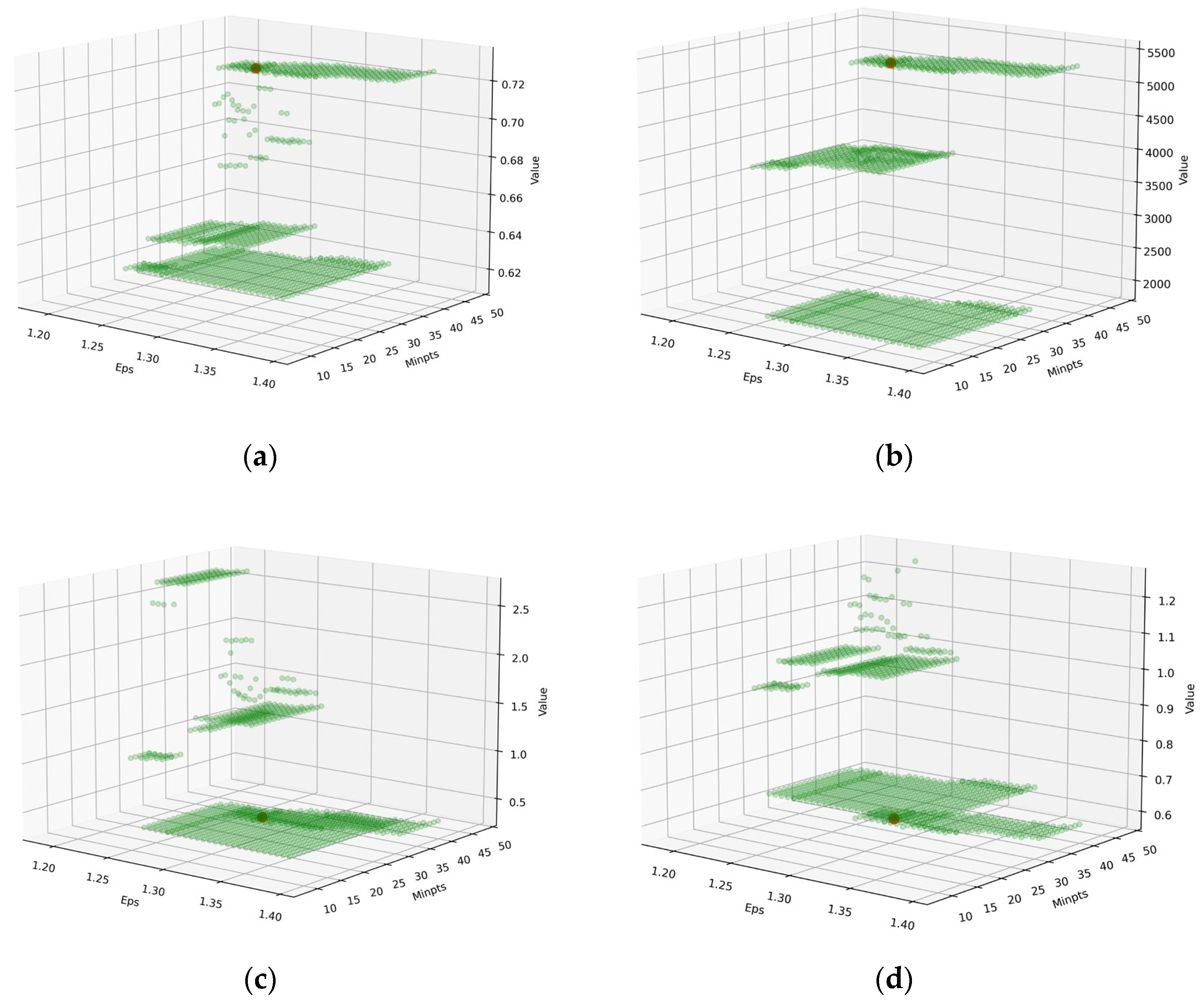
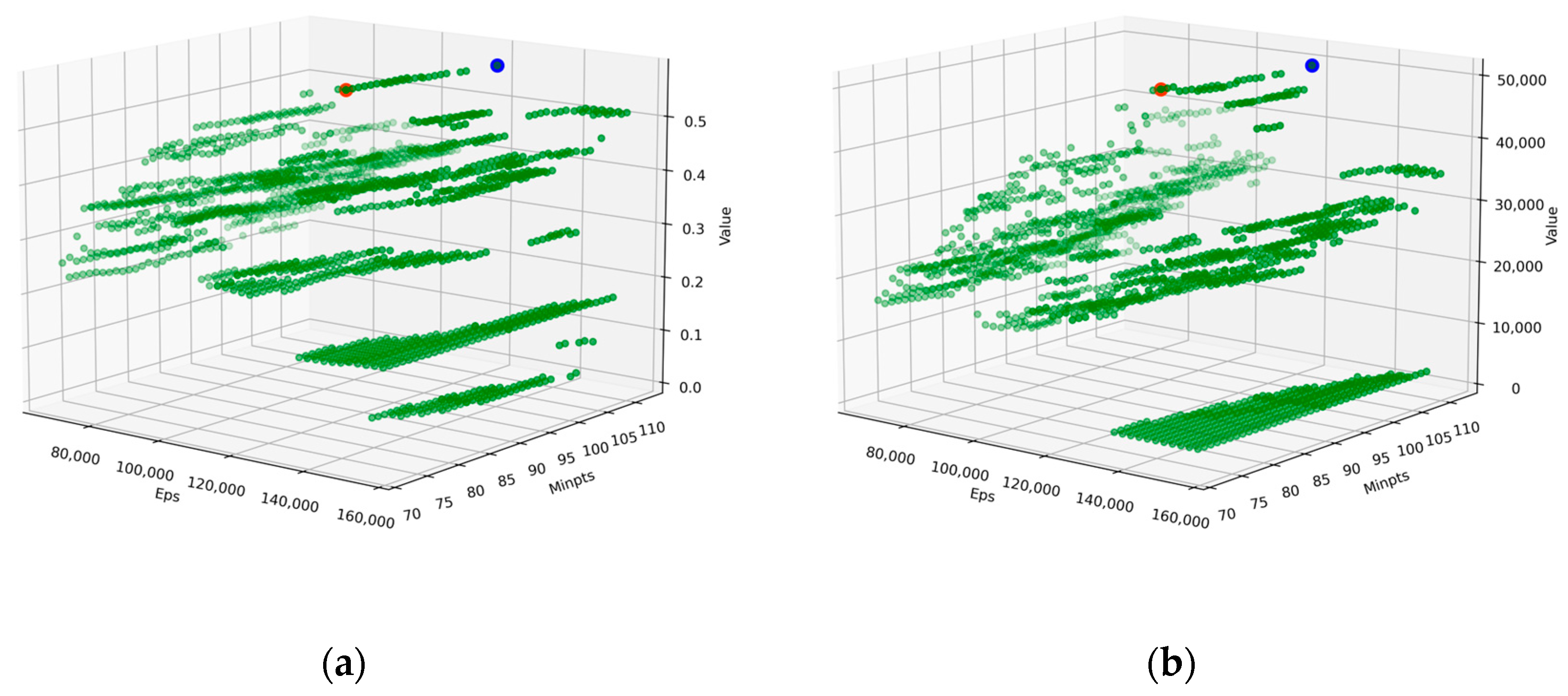
To verify the effectiveness of the dual-population genetic algorithm in identifying relatively optimal threshold values, this study compares clustering results for thresholds near the optimized Eps and MinPts values, within a search range of ±20 steps. The clustering outcomes are evaluated using the Calinski-Harabasz index (CH), Davies-Bouldin index (DB), and SD validity index (SD) as comprehensive performance metrics. The minimum distance between sample points is calculated as 0.005, which is used as the search step for Eps, while the search step for MinPts is set to 1. Threshold combinations that do not satisfy DBSCAN clustering conditions are excluded from the analysis. The final comparison of evaluation metrics is presented in Figure 5, where the red dot in each figure represents the indicator value using the optimized thresholds obtained in this study, and the green dots are the values using all threshold values generated by the stepwise search. The results demonstrate that, within the search region, the dual-population genetic algorithm identifies the threshold combination that produces the best performance. Additionally, for the other reference indices, the optimized thresholds achieve the best score in the CH. In the case of the DB, the difference in ratio between the optimized threshold score and the best DB threshold score is 0.000099, and the difference in ratio for the SD is 0.007759. These indicators demonstrate that the dual-population genetic algorithm can effectively identify high-quality threshold values.

4.2. Experiment Results of Vegetation Fire Point Clustering

In clustering vegetation fire points, two initial populations, each containing 45 randomly generated threshold pairs, are initialized for the dual-population genetic algorithm. The range for Eps is set to [10,000, 200,000], and the range for MinPts is set to (1, 100]. The maximum number of iterations is fixed at 15.
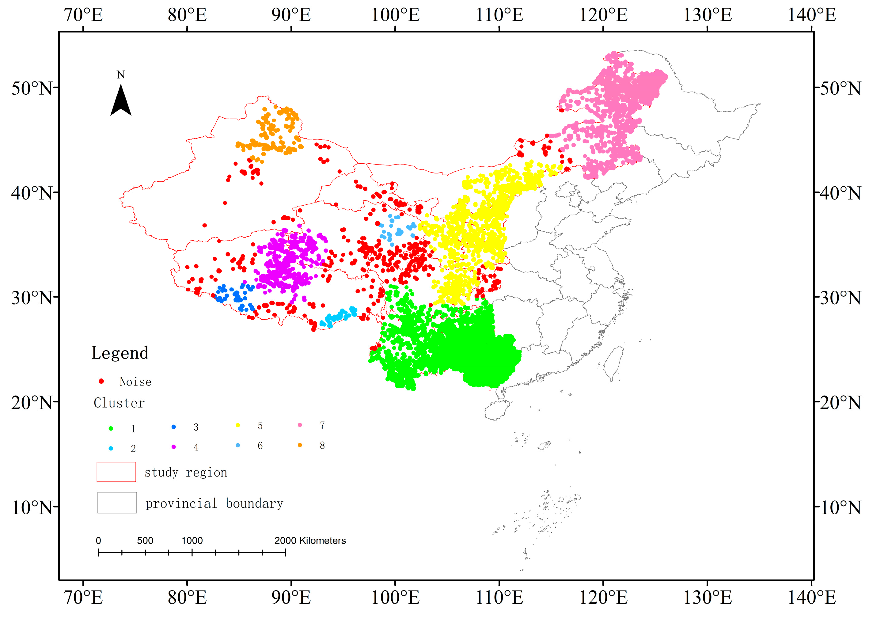
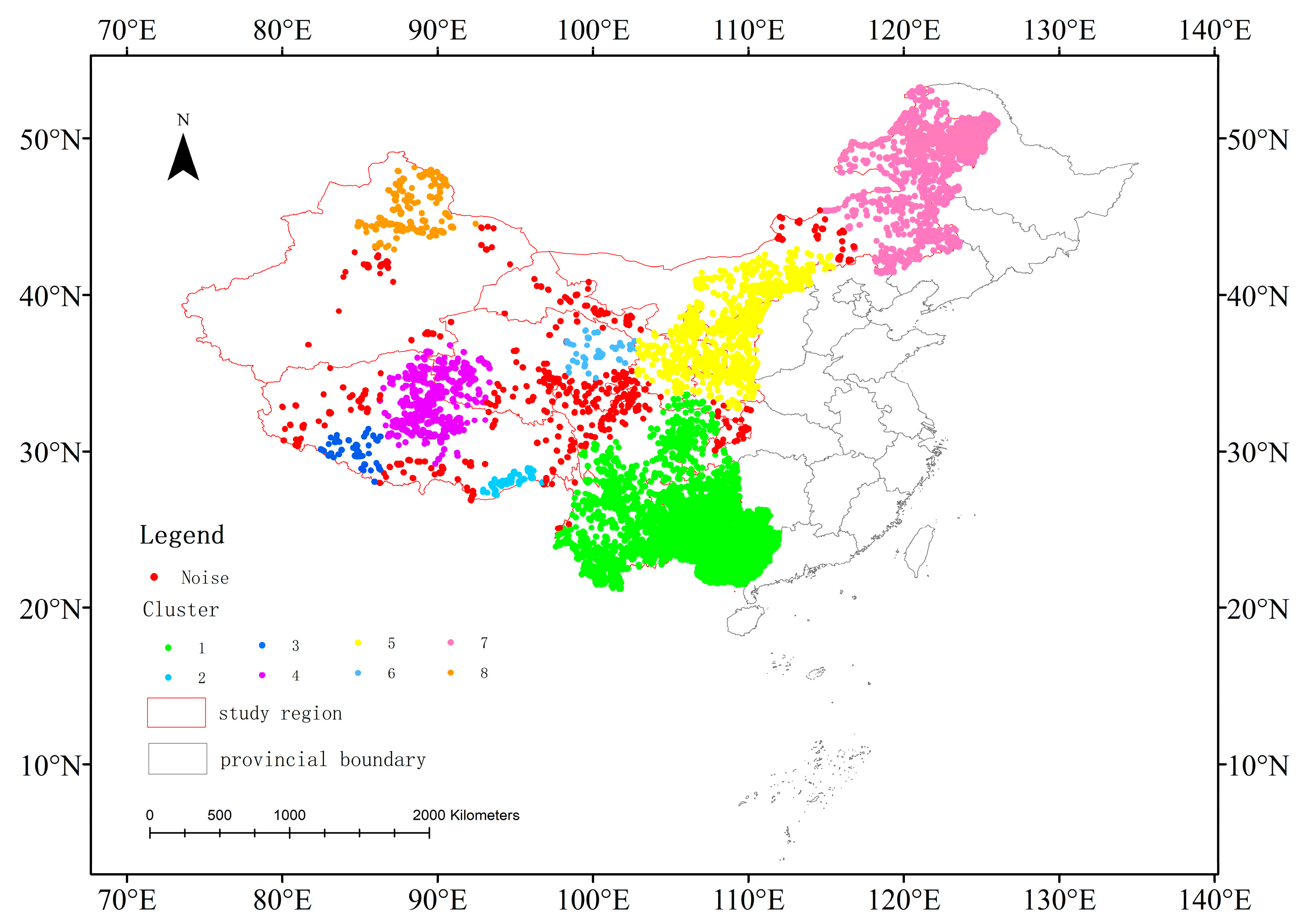
The dataset incorporates multi-year fire detection records, containing instances of fire points detected at identical geographic coordinates across different temporal observations. To optimize computational efficiency, only the first fire occurrence point remains, and other duplicate fire points sharing identical spatial coordinates are removed during preprocessing. After optimizing the threshold selection, the resulting Eps is 111,538, and MinPts is 92. The total number of clusters is 8, with 1250 noise points. The clustering results are shown in Figure 6.
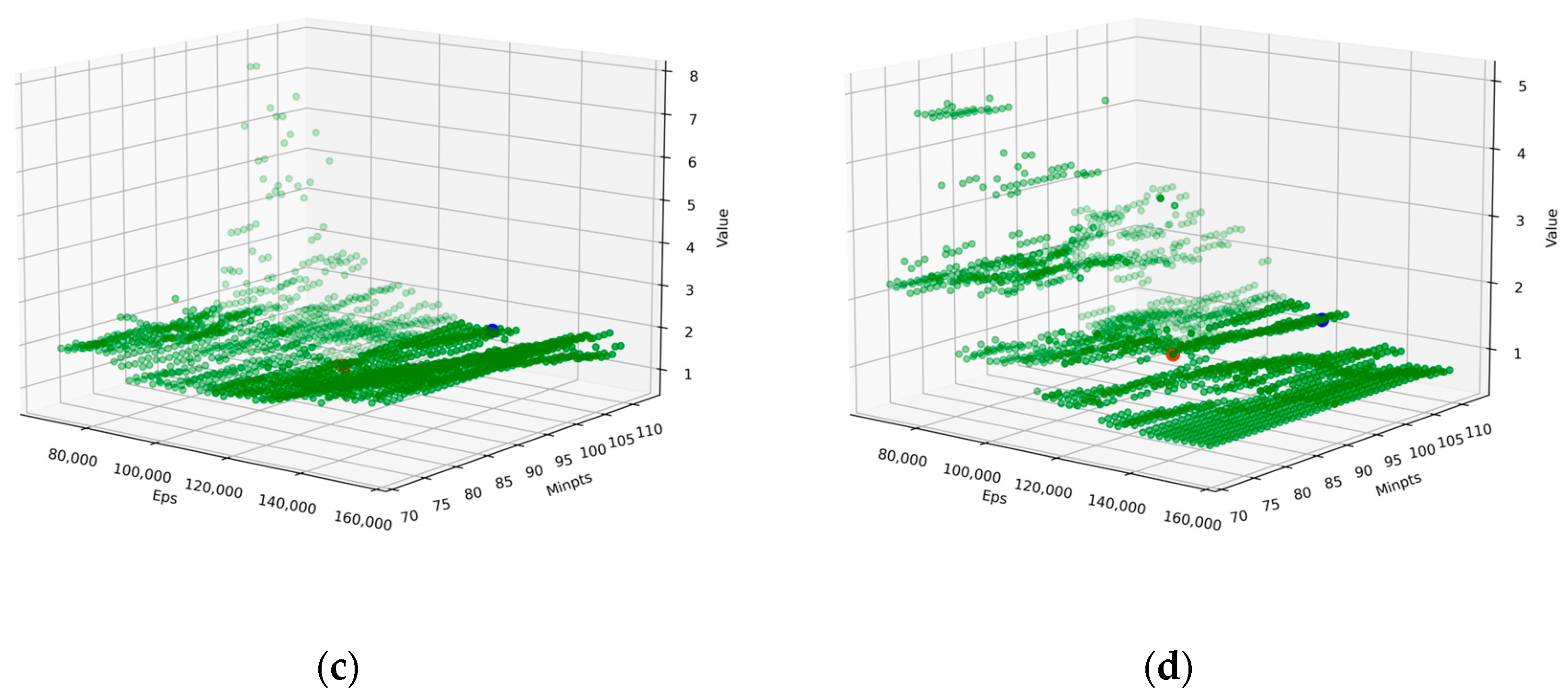
The minimum distance between all unique vegetation fire points is 2226.389 m. Using the optimized thresholds as the center, the search is performed with a step of 2226.389 for Eps and a step of 1 for MinPts. The search is conducted for Eps and MinPts within ±20 steps. MinPts stops if it reaches 2 during the negative-direction search. Similarly, the CH, DB, and SD are used as reference metrics. The scatter plots for each of these indicators are shown in Figure 7, where the red dot in each figure represents the indicator value using the optimized thresholds obtained in this study, the blue dot represents the best fitness score thresholds within the search region, and green dots are the values using all other threshold values generated by stepwise searches.
The blue dot represents a threshold with Eps of 120,443.556 and MinPts of 112. The total number of clusters is also 8, with 1225 noise points. The clustering result is shown in Figure 8. The metrics are compared in Table 1.
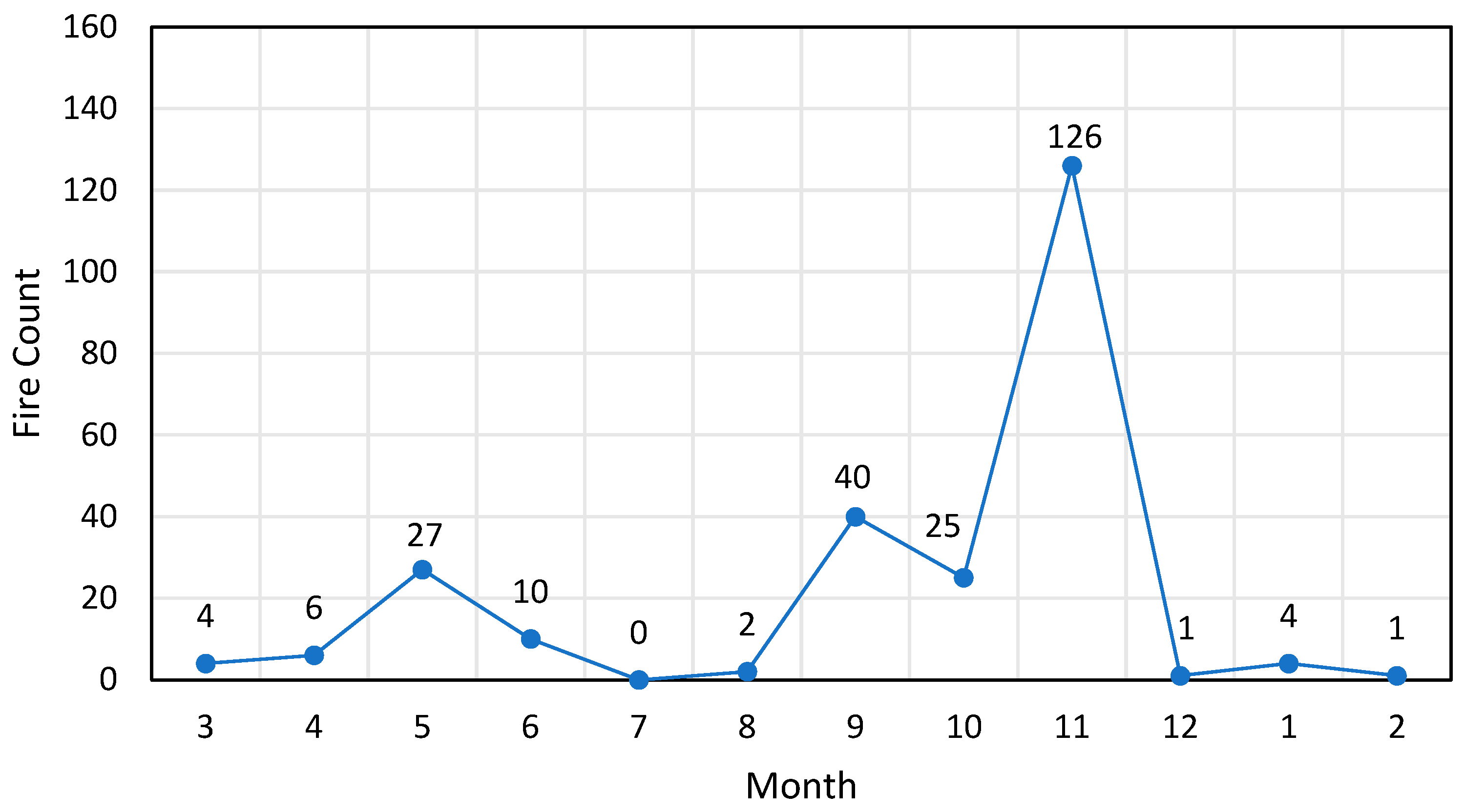
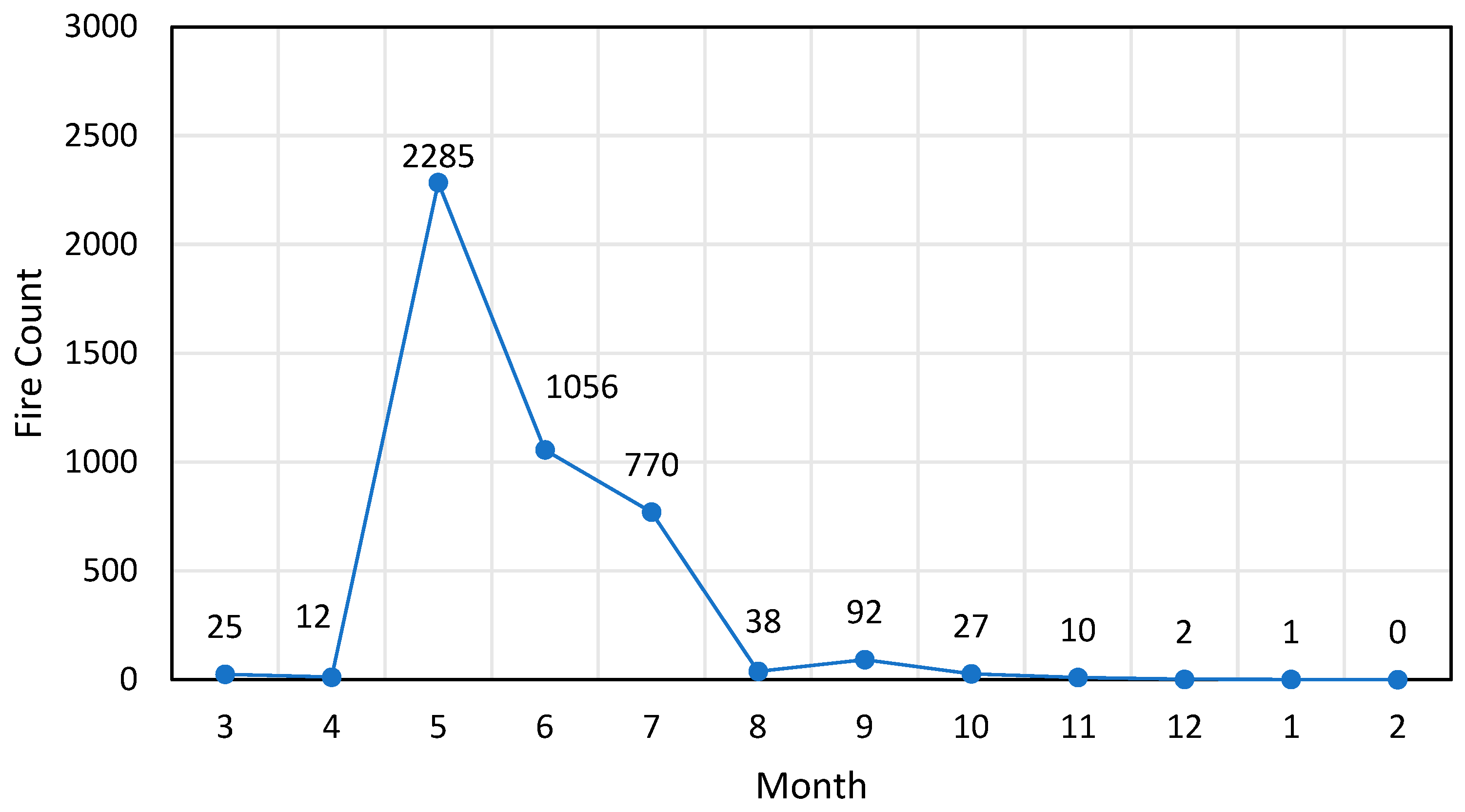
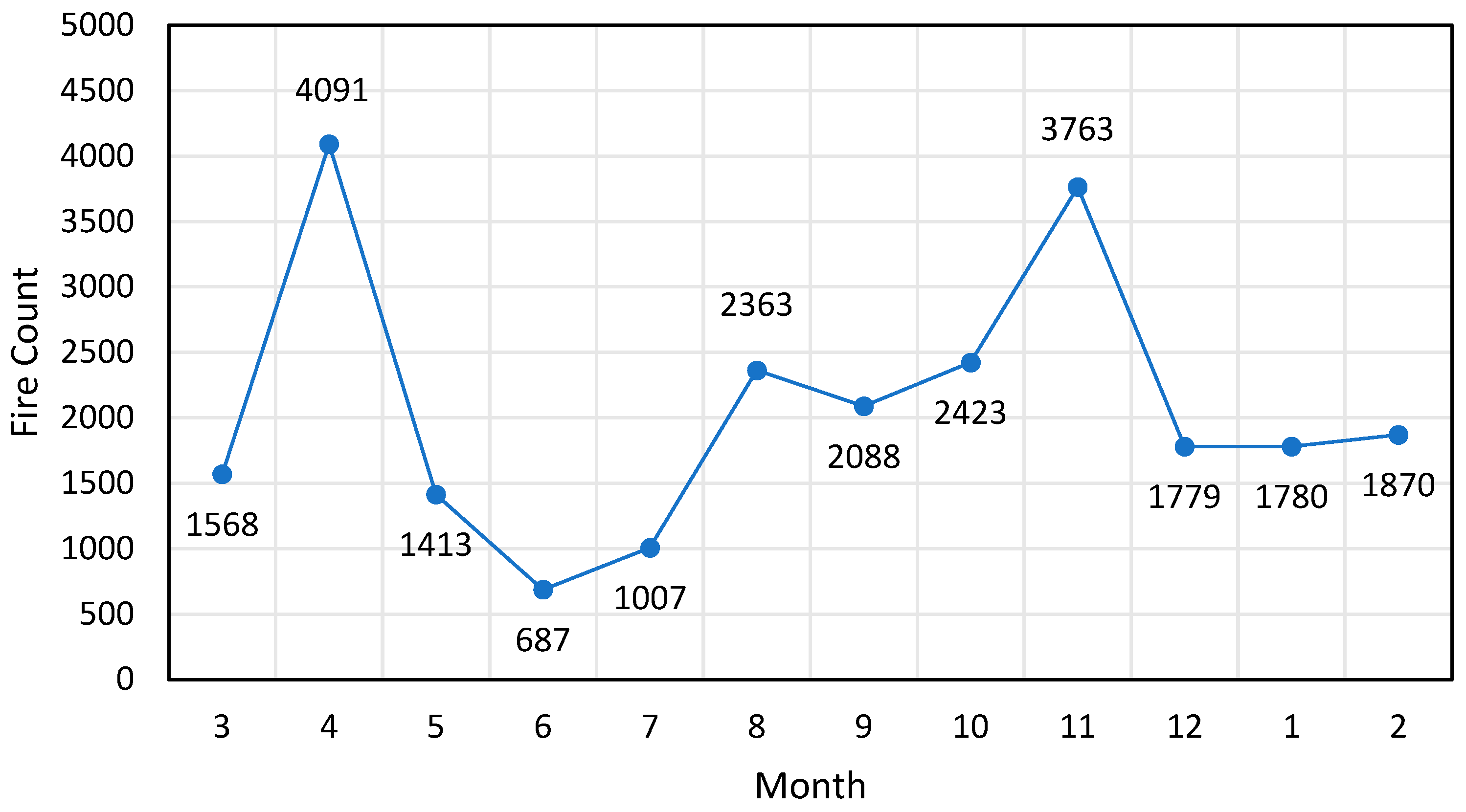
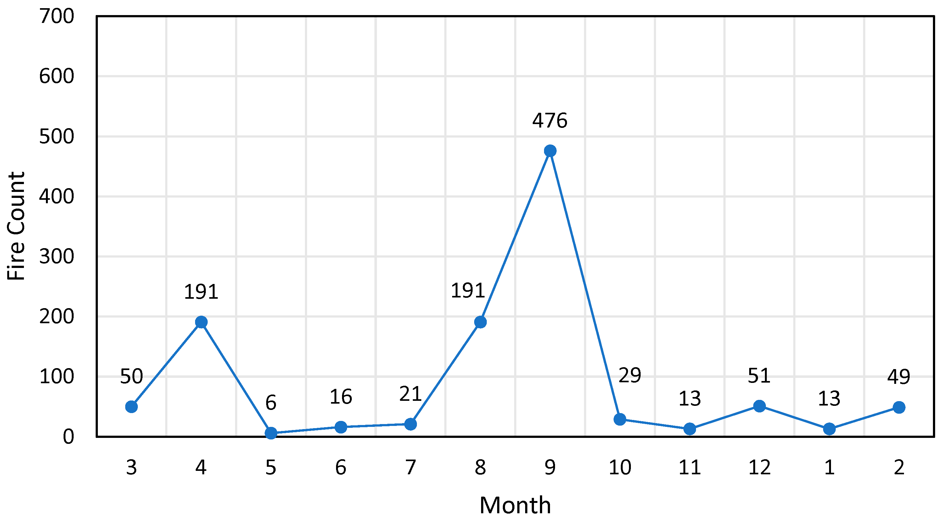
From the clustering results presented in Figure 6 and Figure 8, it is evident that the fire points in western China can be categorized into eight major regions. The cluster-assigned categorical identifiers were propagated back to the source fire point records upon completion of the spatial clustering process. To further investigate the spatiotemporal distribution patterns of these fires, this study analyzes the frequency of wildfire occurrences across different seasons for each area, as summarized in Table 2. It can be seen that winter is the peak season of fires in area 1. Spring is the peak season of fires in areas 2, 4, 5, and 8. Autumn is the peak season of fires in areas 3, 5, 6, and 7. Summer is another peak season of fires in areas 5 and 8.

5. Discussion

Vegetation fires pose ever-increasing threats to the environment and human beings in the background of climate change and expanding anthropogenic activities. Investigating regional clustering patterns of vegetation fire occurrences can help researchers, practitioners, and public policy makers better understand, prepare, and mitigate fire risks with appropriate measures. DBSCAN can group the fire points based on spatial density without specifying the number of clusters. However, the two threshold values, Eps and MinPts, used in DBSCAN are typically determined based on users’ understanding of the geographic conditions of vegetation fire occurrences. Researchers have been working on approaches to find an optimal threshold value. In this paper, a dual-population genetic algorithm is introduced to determine optimal threshold values.
In the comparison of clustering metrics between the result based on this genetic algorithm and that based on stepwise searching of threshold values, the silhouette index performs better in the genetic algorithm approach, since it is the fitness function. Concerning the other three validation metrics, the DB and SD obtained with the genetic optimization approach are better than those obtained with the stepwise search strategy. CH is lower by about 0.5%. The clustering results reveal that fire points in western China can be divided into eight major clusters, each bearing distinct geographic environmental factors and exhibiting different temporal patterns of fire occurrences.
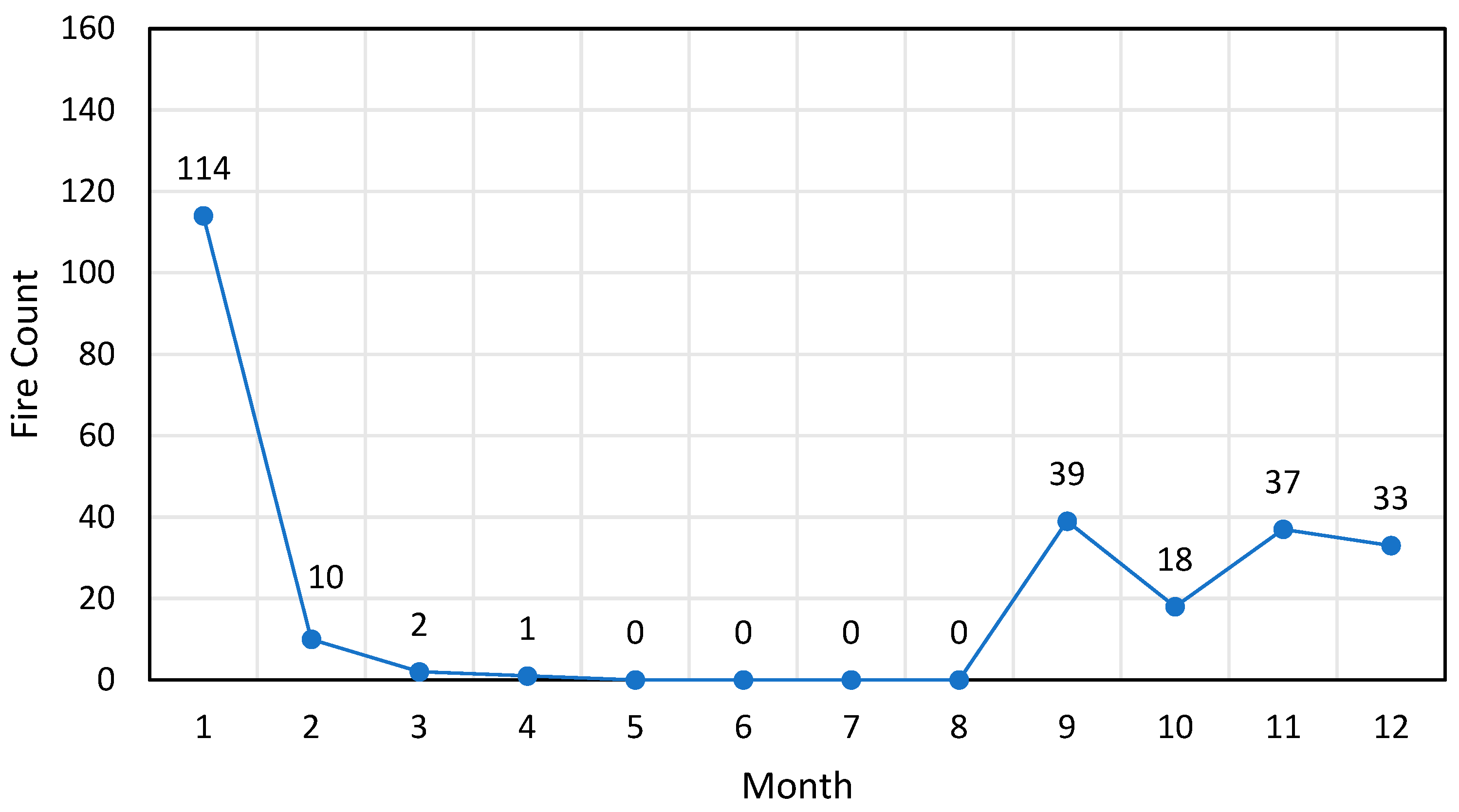
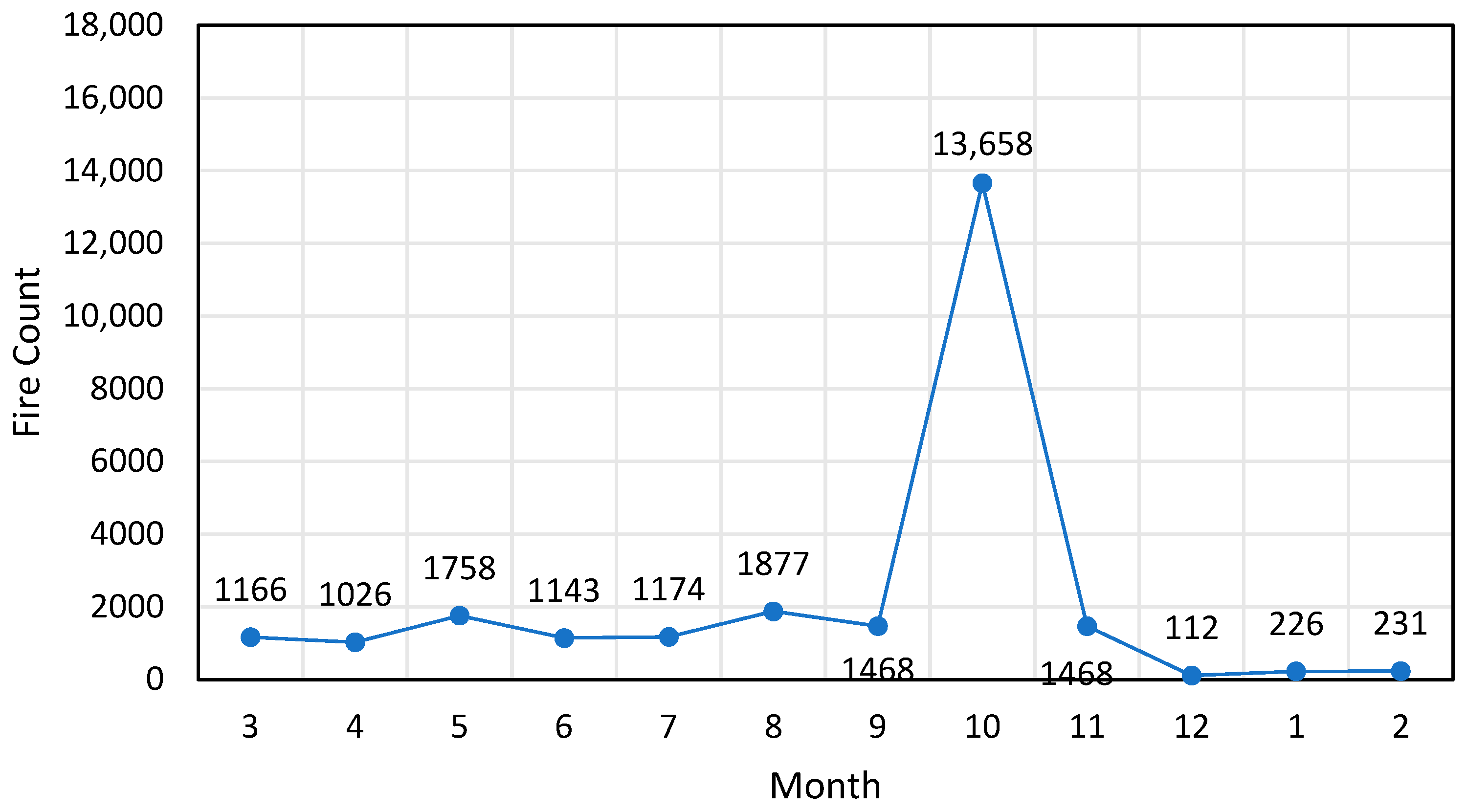
Area 1 (corresponding to the first cluster) encompasses the southern parts of Sichuan, Guizhou, Yunnan, and Guangxi. The region is characterized by dense forests and is influenced by dry continental monsoons during winter, resulting in low rainfall. In winter, the moisture of combustible materials decreases, making the area highly susceptible to fires (Figure 9).
Area 2 is primarily located in southern Tibet, which is densely vegetated. Winter experiences an increase in vegetation fires compared to summer and fall (Figure 10). From February to March, the weather transitions from the cool season to the hot season. Rising temperatures and limited rainfall during this period increase the likelihood of fires.
Area 3 is primarily on the west side of area 2. In this region, after the retreat of the monsoon season, precipitation decreases sharply, leading to the accumulation of dry branches and fallen leaves of trees, which significantly increases the amount of combustible material (Figure 11).
Area 4 is located in the Qinghai–Tibet Plateau, which is dominated by grassland animal husbandry. From late spring to early summer, the region experiences dry and cold weather and growing outdoor anthropogenic activities. The demand for heating increases, leading to a higher incidence of human-induced fires (Figure 12).
Area 5 covers the central and western parts of Inner Mongolia, Shaanxi, and Gansu, where forests have been growing remarkably during the last twenty years [28]. During spring, dry and strong northern winds prevail, leading to low humidity and reduced surface moisture. During autumn, reduced precipitation creates favorable conditions for wildfire risks (Figure 13).
Area 6 is situated in the northeastern part of Qinghai Province. The autumn season witnesses the full retreat of the East Asian monsoon system, leading to precipitous declines in precipitation that induce rapid vegetation senescence. This phenological transition creates highly flammable fuel conditions. Simultaneously, enhanced mid-latitude westerlies provide critical spread potential, dramatically increasing the risks of vegetation fires (Figure 14).
Area 7 is primarily located in eastern Inner Mongolia, which can be taken as Northeastern China geographically. During autumn, grasses and trees dry out, and herders cut grass for winter storage. Increased outdoor activities and the frequent use of fire contribute to a higher incidence of fire hazards (Figure 15).
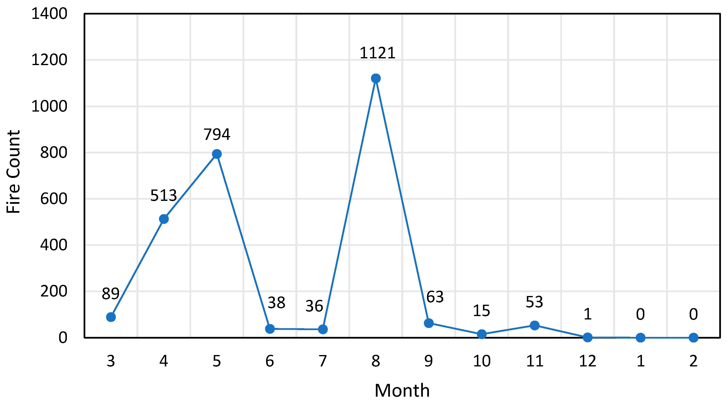
Area 8 is situated in northern Xinjiang, where spring snowmelt driven by rising temperatures promotes vegetation growth. By summer, the Altay Mountains experience a high incidence of lightning-induced wildfires (Figure 16).

6. Conclusions

Based on the DBSCAN clustering method, this study proposes a dual-population genetic algorithm to optimize the selection of the two threshold values. After validating the result using a synthetic dataset, it is applied to vegetation fire data from western China. By comparing three performance metrics of clustering results obtained through stepwise search over feasible threshold ranges, the study demonstrates that the dual-population genetic algorithm can effectively identify relatively optimal threshold values for DBSCAN clustering of vegetation fire points. Temporal analysis of identified clusters shows that each region exhibits unique monthly patterns. Policy makers in different regions can develop tailored prevention measures based on distinct vegetation fire characteristics, tailored to regional fire patterns. Still, there are a number of gaps that can further improve the understanding of vegetation fires.
First, the Himawari-8 wildfire data used in this work features high temporal resolution and broad applicability. Future works need to address the limitations of its relatively low spatial resolution, which cannot report small-scale fires. This research filtered fire points using high confidence levels. However, more considerations concerning the interference of cloud cover and dense smoke should be taken. The advancement of satellite data processing methods has led to numerous novel wildfire detection approaches. For instance, the multi-scale spatio-temporal feature (MSSTF) model utilizes Himawari-8/9 satellite data to enable efficient and robust near-real-time wildfire detection [45]. Furthermore, Multiple data sources, especially remote sensing data, can be helpful in this case, for example, using dNBR (differenced Normalized Burn Ratio) based on higher resolution remote sensing data [46].
Secondly, the study area in this work covers a vast latitudinal range with complex topography, diverse climates, and significant human activities. Evaluation of the clustering results indicates that the classification metrics are near optimal. In subsequent research, the applicability in other regions can be evaluated.
Thirdly, the DBSCAN clustering method determines cluster structures based on the sample density distribution. While it uses a global threshold to identify core points within clusters, it does not account for local density variations. One threshold value setting may not be effective in identifying clusters with varying densities in different parts. It is necessary to introduce a strategy for generating multiple threshold values representing a neighborhood radius adaptive to the local densities. In addition, outliers or noise points generated by the DBSCAN clustering do not belong to any resulting clusters and may not be real noise. These noise points, which do not meet the global threshold but are spatially related to nearby clusters, can affect clustering evaluation metrics. Therefore, future work can also consider how to group some outliers with neighboring clusters, which may further improve clustering accuracy and reliability.
Fourthly, the current clustering results provide a preliminary analysis of fire patterns across different areas. However, from a global perspective, phenomena such as El Niño can also exert influence on vegetation fires in China [47]. Therefore, in subsequent studies, other spatial analysis methods, such as geographic weighted regression models, can be employed to investigate specific correlations between each individual fire cluster and topography, meteorology, vegetation, human activities, and other influencing factors. Based on such models, fire risk intensity distribution maps [48] can be generated to further elucidate the formation mechanisms and occurrence clustering patterns of fires across different regions.

Author Contributions

Conceptualization, X.G. and T.W.; formal analysis, X.G. and T.W.; funding acquisition, T.W.; investigation, X.G.; methodology, X.G. and T.W.; project administration, T.W.; resources, T.W.; supervision, T.W.; validation, X.G. and K.X.; writing—original draft, X.G. and T.W.; writing—review and editing, X.G., T.W. and K.X. All authors will be updated at each stage of manuscript processing, including submission, revision, and revision reminder, via emails from our system or the assigned Assistant Editor. All authors have read and agreed to the published version of the manuscript.

Funding

This research is partly supported by the National Natural Science Foundation of China (Grant No. 42471464).

Institutional Review Board Statement

Not applicable.

Informed Consent Statement

Not applicable.

Data Availability Statement

The data presented in this study are available on request from the corresponding author.

Conflicts of Interest

The authors declare no conflicts of interest.

References

  1. Scholten, R.C.; Veraverbeke, S.; Chen, Y.; Randerson, J.T. Spatial variability in Arctic-boreal fire regimes influenced by environmental and human factors. Nat. Geosci. 2024, 17, 866–873. [Google Scholar] [CrossRef]
  2. Jolly, W.M.; Cochrane, M.A.; Freeborn, P.H.; Holden, Z.A.; Brown, T.J.; Williamson, G.J.; Bowman, D.M. Climate-induced variations in global wildfire danger from 1979 to 2013. Nat. Commun. 2015, 6, 7537. [Google Scholar] [CrossRef]
  3. Bal, Y.; Wang, B.; Wu, Y.D.; Liu, X.D. A review of global forest fires in 2021. Fire Sci. Technol. 2022, 41, 705–709. [Google Scholar]
  4. Brys, C.; Martínez, D.; Marinelli, M. Machine learning methods for wildfire risk assessment. Earth Sci. Inform. 2025, 18, 148. [Google Scholar] [CrossRef]
  5. Bowman, D.M.; Kolden, C.A.; Abatzoglou, J.T.; Johnston, F.H.; van der Werf, G.R.; Flannigan, M. Vegetation fires in the Anthropocene. Nat. Rev. Earth Environ. 2020, 1, 500–515. [Google Scholar] [CrossRef]
  6. van der Werf, G.R.; Randerson, J.T.; Giglio, L.; van Leeuwen, T.T.; Chen, Y.; Rogers, B.M.; Mu, M.; van Marle, M.J.E.; Morton, D.C.; Collatz, G.J.; et al. Global fire emissions estimates during 1997–2016. Earth Syst. Sci. Data 2017, 9, 697–720. [Google Scholar] [CrossRef]
  7. Li, S.; Meng, C.; Zhu, Y.P. Temporal and spatial distribution of economic losses and casualties of forest fires in China. Fire Sci. Technol. 2023, 42, 387–391. [Google Scholar]
  8. Yi, K.; Bao, Y.; Zhang, J. Spatial distribution and temporal variability of open fire in China. Int. J. Wildland Fire 2016, 26, 122–135. [Google Scholar] [CrossRef]
  9. Donovan, V.M.; Crandall, R.; Fill, J.; Wonkka, C.L. Increasing large wildfire in the eastern United States. Geophys. Res. Lett. 2023, 50, e2023GL107051. [Google Scholar] [CrossRef]
  10. Reddy, C.S.; Bird, N.G.; Sreelakshmi, S.; Manikandan, T.M.; Asra, M.; Krishna, P.H.; Jha, C.S.; Rao, P.V.N.; Diwakar, P.G. Identification and characterization of spatio-temporal hotspots of forest fires in South Asia. Environ. Monit. Assess. 2020, 191 (Suppl. 3), 791. [Google Scholar] [CrossRef]
  11. Feltman, J.A.; Straka, T.J.; Post, C.J.; Sperry, S.L. Geospatial Analysis Application to Forecast Wildfire Occurrences in South Carolina. Forests 2012, 3, 265–282. [Google Scholar] [CrossRef]
  12. Prasertsri, N.; Littidej, P. Spatial Environmental Modeling for Wildfire Progression Accelerating Extent Analysis Using Geo-Informatics. Pol. J. Environ. Stud. 2020, 29, 3249–3261. [Google Scholar] [CrossRef] [PubMed]
  13. Brunsdon, C.; Fotheringham, A.S.; Charlton, M.E. Geographically weighted regression: A method for exploring spatial nonstationarity. Geogr. Anal. 1996, 28, 281–298. [Google Scholar] [CrossRef]
  14. Ma, C.; Pu, R.; Downs, J.; Jin, H. Characterizing Spatial Patterns of Amazon Rainforest Wildfires and Driving Factors by Using Remote Sensing and GIS Geospatial Technologies. Geosciences 2022, 12, 237. [Google Scholar] [CrossRef]
  15. Bhadoria, R.S.; Pandey, M.K.; Kundu, P. RVFR: Random vector forest regression model for integrated & enhanced approach in forest fires predictions. Ecol. Inform. 2021, 66, 101471. [Google Scholar]
  16. Li, Z.Y.; Chen, E.X.; Guo, Y.; Tian, X.; Liu, Q.W.; Sun, B.; Zhao, L.; Cai, X.S.; Du, L.M.; Yu, L.F.; et al. Research and application of forestry and grassland remote sensing technology in China: Recent progress, challenges and countermeasures. Natl. Remote Sens. Bull. 2025, 29, 1804–1830. [Google Scholar]
  17. Grubesic, T.H.; Wei, R.; Murray, A.T. Spatial Clustering Overview and Comparison: Accuracy, Sensitivity, and Computational Expense. Ann. Assoc. Am. Geogr. 2014, 104, 1134–1156. [Google Scholar] [CrossRef]
  18. Varghese, B.; Unnikrishnan, A.; PouloseJacob, K. Spatial clustering algorithms-an overview. Asian J. Comput. Sci. Inf. Technol. 2013, 3, 1–8. [Google Scholar]
  19. Hohl, A.; Zheng, M.; Tang, W.; Delmelle, E.; Casas, I. Spatiotemporal Point Pattern Analysis Using Ripley’s K Function. Geospatial Data Science Techniques and Applications, 1st ed.; Karimi, H.A., Karimi, B., Eds.; Taylor & Francis Group: Oxford, UK, 2018; pp. 155–176. [Google Scholar]
  20. Tian, Y.; Wu, Z.; Bian, S.; Zhang, X.; Wang, B.; Li, M. Study on spatial-distribution characteristics based on fire-spot data in Northern China. Sustainability 2022, 14, 6872. [Google Scholar] [CrossRef]
  21. Baykal, T.M. Performance assessment of GIS-based spatial clustering methods in forest fire data. Nat. Hazards 2025, 121, 8445–8477. [Google Scholar] [CrossRef]
  22. Khairani, N.A.; Sutoyo, E. Application of K-Means Clustering Algorithm for Determination of Fire-Prone Areas Utilizing Hotspots in West Kalimantan Province. Int. J. Adv. Data Inf. Syst. 2020, 1, 9–16. [Google Scholar] [CrossRef]
  23. Ester, M.; Kriegel, H.P.; Sander, J.; Xu, X.W. A density-based algorithm for discovering clusters in large spatial databases with noise. In Proceedings of the 2nd International Conference on Knowledge Discovery and Data Mining (KDD), Menlo Park, CA, USA, 2–4 August 1996; pp. 226–231. [Google Scholar]
  24. Gan, J.; Tao, Y. DBSCAN revisited: Mis-claim, un-fixability, and approximation. In Proceedings of the SIGMOD ‘15: Proceedings of the 2015 ACM SIGMOD International Conference on Management of Data, New York, NY, USA, 27 May 2015; pp. 519–530. [Google Scholar]
  25. Ahajjam, A.; Allgaier, M.; Chance, R.; Chukwuemeka, E.; Putkonen, J.; Pasch, T. Enhancing prediction of wildfire occurrence and behavior in Alaska using spatio-temporal clustering and ensemble machine learning. Ecol. Inf. 2025, 85, 102963. [Google Scholar] [CrossRef]
  26. Song, M.; Chen, D.M. A Comparison of Three Heuristic Optimization Algorithms for Solving the Multi-Objective Land Allocation (MOLA) Problem. Ann. GIS 2018, 24, 19–31. [Google Scholar] [CrossRef]
  27. Gebril, I.H.; El-Mouadib, F.A.; Mansori, H.A. Automatic Generation of Epsilon (Eps) value for DBSCAN Using Genetic Algorithms. In Proceedings of the 2024 IEEE 4th International Maghreb Meeting of the Conference on Sciences and Techniques of Automatic Control and Computer Engineering (MI-STA), Tripoli, Libya, 19–21 May 2024. [Google Scholar]
  28. Wei, X.; Liu, R.; Liu, Y.; He, J.; Chen, J.; Qi, L.; Zhou, Y.; Qin, Y.; Wu, C.; Dong, J.; et al. Forest areas in China are recovering since the 21st century. Geophys. Res. Lett. 2024, 51, e2024GL110312. [Google Scholar] [CrossRef]
  29. Yin, J.; He, B.; Fan, C.; Chen, R. Fire has become a major disturbance agent in the forests of Southwest China. Ecol. Indic. 2024, 160, 111885. [Google Scholar] [CrossRef]
  30. Li, W.; Shu, L.F.; Wang, M.Y.; Li, W.K.; Yuan, S.B.; Si, L.Q.; Zhao, F.J.; Song, J.J.; Wang, Y.H. Temporal and Spatial Distribution and Dynamic Characteristics of Lightning Fires in the Daxing’anling Mountains from 1980 to 2021. Sci. Silvae Sin. 2023, 59, 22–31. [Google Scholar]
  31. Zhang, J.H.; Wang, X.J.; Qian, Y.H.; Pei, S.Y. Environmental factor analysis of grassland fire in Qinghai Province. J. Nat. Disasters 2007, 16, 71–75. [Google Scholar]
  32. Zhou, W.; Tang, B.H.; He, Z.W.; Huang, L.; Chen, J. Identification of forest fire points under clear sky conditions with Himawari-8 satellite data. Int. J. Remote Sens. 2024, 45, 214–234. [Google Scholar] [CrossRef]
  33. Na, L.; Zhang, J.; Bao, Y.; Bao, Y.; Na, R.; Tong, S.; Si, A. Himawari-8 Satellite Based Dynamic Monitoring of Grassland Fire in China-Mongolia Border Regions. Sensors 2018, 18, 276. [Google Scholar] [CrossRef]
  34. Zhang, D.; Huang, C.; Gu, J.; Hou, J.; Zhang, Y.; Han, W.; Dou, P.; Feng, Y. Real-Time Wildfire Detection Algorithm Based on VIIRS Fire Product and Himawari-8 Data. Remote Sens. 2023, 15, 1541. [Google Scholar] [CrossRef]
  35. Scikit-Learn. Available online: https://scikit-learn.org/ (accessed on 23 October 2025).
  36. Holland, J.H. Adaptation in Natural and Artificial Systems: An Introductory Analysis with Applications to Biology, Control, and Artificial Intelligence; The MIT Press: Cambridge, MA, USA, 1992. [Google Scholar]
  37. Golberg, D.E. Genetic algorithms in search, optimization, and machine learning. Addion Wesley 1989, 27, 27–0936. [Google Scholar]
  38. Park, J.; Park, M.-W.; Kim, D.-W.; Lee, J. Multi-Population Genetic Algorithm for Multilabel Feature Selection Based on Label Complementary Communication. Entropy 2020, 22, 876. [Google Scholar] [CrossRef] [PubMed]
  39. Hong, J.; Shi, L.; Du, K.J.; Chen, C.H.; Wang, H.; Zhang, J.; Zhan, Z.H. A Multi-Population Genetic Algorithm for Multiobjective Recommendation System. In Proceedings of the 2023 IEEE Symposium Series on Computational Intelligence (SSCI), Mexico City, Mexico, 5–8 December 2023; pp. 998–1003. [Google Scholar]
  40. Shahapure, K.R.; Nicholas, C. Cluster Quality Analysis Using Silhouette Score. In Proceedings of the 2020 IEEE 7th International Conference on Data Science and Advanced Analytics (DSAA), Sydney, Australia, 6–9 October 2020. [Google Scholar]
  41. Rousseeuw, P. Silhouettes: A graphical aid to the interpretation and validation of cluster analysis. J. Comput. Appl. Math. 1987, 20, 53–65. [Google Scholar] [CrossRef]
  42. Calinski, T.; Harabasz, J. A dendrite method for cluster analysis. Comm. Stat. 1974, 3, 1–27. [Google Scholar]
  43. Davies, D.; Bouldin, D. A cluster separation measure. IEEE PAMI 1979, 1, 224–227. [Google Scholar] [CrossRef]
  44. Halkidi, M.; Vazirgiannis, M.; Batistakis, Y. Quality scheme assessment in the clustering process. In Proceedings of the PKDD, London, UK, 14–18 September 2000; pp. 265–276. [Google Scholar]
  45. Zhang, L.; Zhang, Q.; Yang, Q.; Yue, L.; He, J.; Jin, X.; Yuan, Q. Near-Real-Time Wildfire Detection Approach with Himawari-8/9 Geostationary Satellite Data Integrating Multi-Scale Spatial-Temporal Feature. Int. J. Appl. Earth Obs. Geoinf. 2025, 137, 104416. [Google Scholar] [CrossRef]
  46. Chen, Y.; Morton, D.C.; Randerson, J.T. Remote sensing for wildfire monitoring: Insights into burned area, emissions, and fire dynamics. One Earth 2024, 7, 1022–1028. [Google Scholar] [CrossRef]
  47. Fang, K.; Yao, Q.; Guo, Z.; Zheng, B.; Du, J.; Qi, F.; Yan, P.; Li, J.; Ou, T.; Liu, J.; et al. ENSO modulates wildfire activity in China. Nat. Commun. 2021, 12, 1764. [Google Scholar] [CrossRef]
  48. Sohel, S.I.; Marshall, A.R. Why the world needs a wildfire risk prediction system based on plant functional traits and moisture-before fires ignite. npj Nat. Hazards 2025, 2, 95. [Google Scholar] [CrossRef]
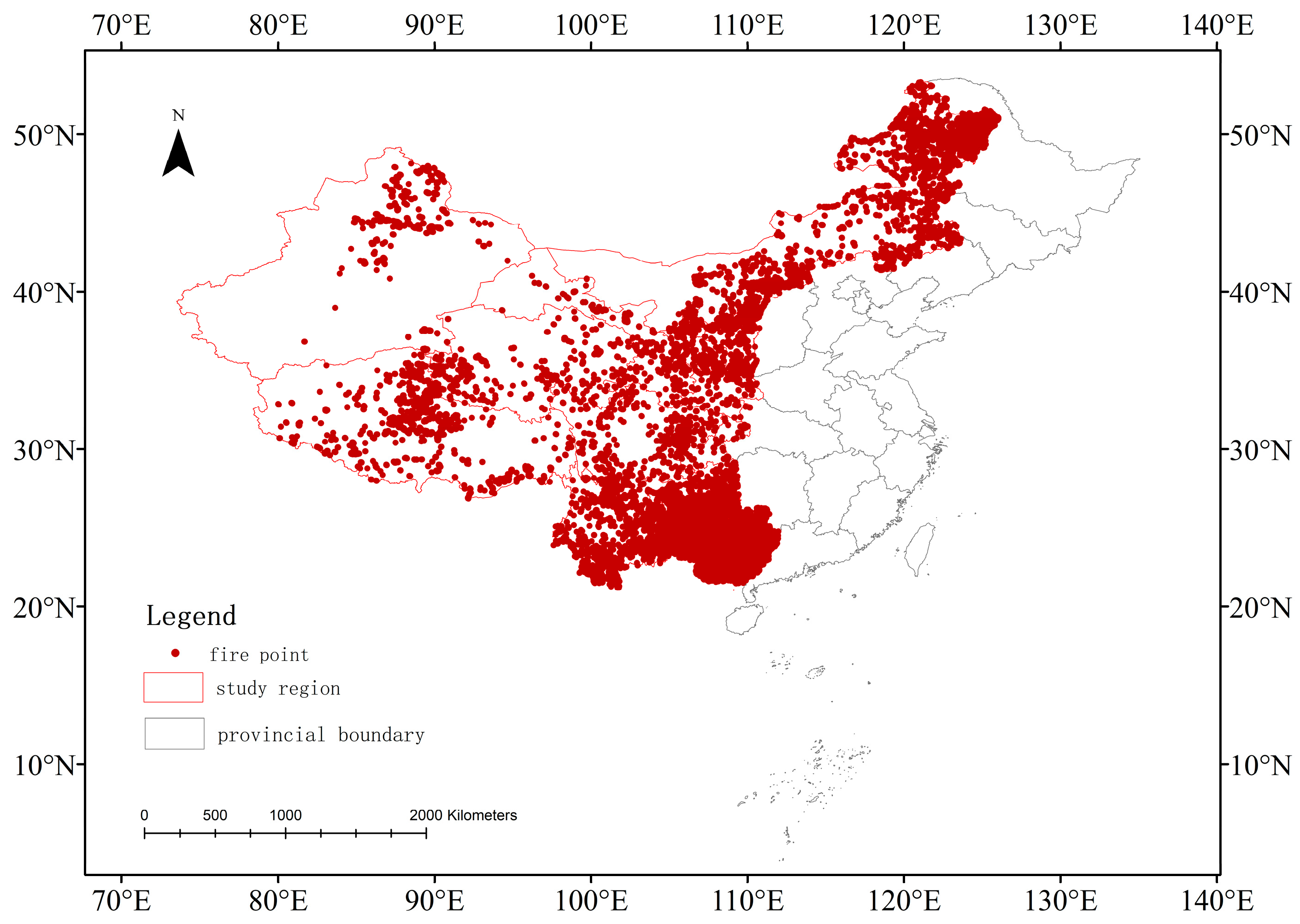
Figure 1. Study area.
Fire 08 00431 g001
Figure 2. Daily statistics of fire points of western China during 2016 and 2022.
Fire 08 00431 g002
Figure 3. Synthetic test dataset.
Fire 08 00431 g003
Figure 4. Clustering result of the synthetic test dataset based on optimized threshold values (each color represents one cluster).
Fire 08 00431 g004
Figure 5. Test dataset scatter plot of thresholds evaluation: (a) silhouette index; (b) Calinski–Harabasz index; (c) Davies–Bouldin index; (d) SD (Scattering/distance) validity index.
Fire 08 00431 g005
Figure 6. Clustering result of fire points based on optimized threshold values.
Fire 08 00431 g006
Figure 7. Fire points scatter plot of threshold evaluation: (a) silhouette index; (b) Calinski–Harabasz index; (c) Davies–Bouldin index; (d) SD (Scattering/distance) validity index.
Fire 08 00431 g007aFire 08 00431 g007b
Figure 8. Clustering result based on the best fitness score threshold values.
Fire 08 00431 g008
Figure 9. Monthly fire spot statistics map for area 1.
Fire 08 00431 g009
Figure 10. Monthly fire spot statistics map for area 2.
Fire 08 00431 g010
Figure 11. Monthly fire spot statistics map for area 3.
Fire 08 00431 g011
Figure 12. Monthly fire spot statistics map for area 4.
Fire 08 00431 g012
Figure 13. Monthly fire spot statistics map for area 5.
Fire 08 00431 g013
Figure 14. Monthly fire spot statistics map for area 6.
Fire 08 00431 g014
Figure 15. Monthly fire spot statistics map for area 7.
Fire 08 00431 g015
Figure 16. Monthly fire spot statistics map for area 8.
Fire 08 00431 g016
Table 1. Comparison of clustering metrics.
Internal IndicesClustering by Genetic Optimized ThresholdsClustering by Stepwise Search Thresholds
S0.561110.56576
CH48,839.1942149,113.84489
DB1.298821.40942
SD1.052761.11991
Table 2. Regional fire points seasonal statistics.
ClusterClustering by Genetic Optimized ThresholdsClustering by Stepwise Search Thresholds
SpringSummerFallWinterSpringSummerFallWinter
14914349376713,1075027462390713,353
21261378812613988
33711186337121916
4232018581253232218641293
572824229841756877072405782745429
6245224489107247228518113
73964419716,5945693950419416,594569
8139411931311139611951311
Disclaimer/Publisher’s Note: The statements, opinions and data contained in all publications are solely those of the individual author(s) and contributor(s) and not of MDPI and/or the editor(s). MDPI and/or the editor(s) disclaim responsibility for any injury to people or property resulting from any ideas, methods, instructions or products referred to in the content.