Abstract
Previous works have shown the effectiveness of EfficientNet—a convolutional neural network built upon the concept of compound scaling—in automatically detecting smoke plumes at a distance of several kilometres in visible camera images. Building on these results, we have created enhanced EfficientNet models capable of precisely identifying the smoke location due to the introduction of a mosaic-like output and achieving extremely reduced false positive percentages due to using partial AUROC and applying class imbalance. Our EfficientNets beat InceptionV3 and MobileNetV2 in the same dataset and achieved a true detection percentage of 89.2% and a false positive percentage of only 0.306% across a test set with 17,023 images. The complete dataset used in this study contains 26,204 smoke and 51,075 non-smoke images. This makes it one of the largest, if not the most extensive, datasets reported in the scientific literature for smoke plume imagery. So, the achieved percentages are not only among the best reported for this application but are also among the most reliable due to the extent and representativeness of the dataset.
1. Introduction
Few natural events possess the destructive potential of wildfires, endangering both wild and human life and significantly threatening human property and the environment. The fire risk increases as populations move closer to wild regions. One way to mitigate this problem is by deploying wildfire detection systems, which may take many forms. The most conventional one is the installation of watchtowers for human-based surveillance over broad regions [1]. New technologies have also been suggested, such as light detection and ranging (LIDAR) [2,3], wireless sensor networks [4], spectrometers [5], satellite and drone-based surveillance [6,7], and crowd sensing [8] through applications. The present work focuses on wildfire detection rather than fire detection in buildings [9,10]. One of the simplest and most effective ways of replacing observers in wildfire watchtowers is by using cameras. By doing so, it is possible to consolidate multiple camera feeds for observation by a single operator in a centralised control room, substantially mitigating the working conditions associated with remote watchtowers.
Surveillance cameras operating with visible light have been developed for various applications with commercial value, which make them inexpensive, robust to the weather, wind, and temperature, and capable of operating 24/7 without much maintenance. This has led to the emergence of various wildfire surveillance systems based on visible cameras: FireWatch [11], ForestWatch [12], SmokeD [13], High-Performance Wireless Research and Education Network (HPWREN) [14], and CICLOPE [15]. In the present work, we are interested in smoke detection with visible cameras strategically positioned at high vantage points. In our opinion, this method is one of the most effective ways of detecting wildfires since flames may not be directly visible due to obstructions; however, smoke tends to rise rapidly above these barriers, offering a more reliable detection indicator.
Knowing field-deployed detection systems’ false positive and true detection percentages is challenging since these values are seldom published, likely due to commercial sensitivities. However, insights into these metrics can be obtained from scientific publications. The difficulty in getting realistic values for these percentages from the scientific literature is the frequent, less-than-desirable amount of data used in evaluations. Indeed, a review of this literature might lead one to believe that there is nothing more to investigate, as the systems are almost perfect. Nevertheless, this is far from the truth, as noted by Peng and Wang [16] in their 2022 article:
“...the existing fire detection algorithm development process often focuses only on the increased fire recognition ability, while ignoring the false alarm rate and generalisation ability of the algorithm, which causes the algorithm to be eventually deprecated by users due to many false positives.”
Recent works have tried to address the issues of limited generalisation ability and the many false positives by significantly increasing the dataset size. Fernandes et al., 2022 [17] and Fernandes et al., 2023 [18] utilised the same dataset composed of 14,125 and 21,203 images with and without smoke to improve the reliability of the created systems. These two works use, to the best of the author’s knowledge, the largest number of images with smoke in the scientific literature on wildfire detection. Their dataset images are also highly realistic due to being captured from various surveillance towers and at large distances from the smoke plumes. It is relatively common to find studies where the fire images are captured at a few metres’ distance or have large visible flames, making them unrealistic for early and long-range wildfire detection [19,20]. The present work continues the trend of increasing the dataset size and keeping it highly realistic by using only images captured in surveillance towers. We use 26,204 and 51,075 images with and without smoke, respectively, representing an increase of 85% and 241% in the number of images relative to the two mentioned articles from Fernandes et al. [17,18]. The current dataset encompasses all images from these two preceding studies.
Regarding the algorithms, in 2022, Fernandes et al. [17] used an EfficientNet-B0 [21] to obtain 85.5% and 3.1% in true and false positives, respectively. In [17], EfficientNet results surpassed those of ResNet. In 2023, Fernandes et al. [18] with EfficientDet-D1 [22], the false positives were improved to 1.13%, with true positives of 80.4%. For the same value of 1.13% of false positives, EfficientNet-B0 exhibited 74% of true detection. Despite the good results with EfficientDet in the past, this study reverts to using EfficientNet and reports an improvement in classification efficiency relative to Fernandes et al. [17,18]. The return occurs because we could not improve the results after some experiments with EfficientDet applied to datasets with images similar to those employed here. EfficientNets excel at surpassing networks of similar size and complexity in classification efficiency. When the trend was to massively increase the number of neural network weights to win the state-of-the-art in the Imagenet dataset, EfficientNet proposed a dramatic decrease in this parameter and still became state-of-the-art [21]. The innovative aspect of our EfficientNets lies in their use of a mosaic-like output, assigning each image region a binary value indicating the presence or absence of smoke, thus enabling smoke plume location with algorithms not originally intended for this purpose. The mosaic was used in Fernandes et al., 2022 [17], but with a less detailed grid for plume location. Using partial area under the receiver operating characteristic curve (pAUROC), combined with a class imbalance in the training set by employing more images without smoke, allowed us to reach significantly lower false positive percentages while keeping good true detection percentages. The present work compares EfficientNets with InceptionV3 and MobileNetV2, as both Govil et al. [23] and Gonçalves et al. [24] reported favourable results using these models on images similar to ours.
The subsequent sections of the article include the following: “Materials and Methods”, where the dataset and the algorithms employed in the research are described; “Results”, which presents and characterises the various machine learning models created and selects the best one; “Discussion”, which gives details about the class imbalance in training, possible cases of misdetections (false negatives) and false positives, and makes a comparison to other works; and finally, the conclusive section.
2. Materials and Methods
2.1. Sample Description
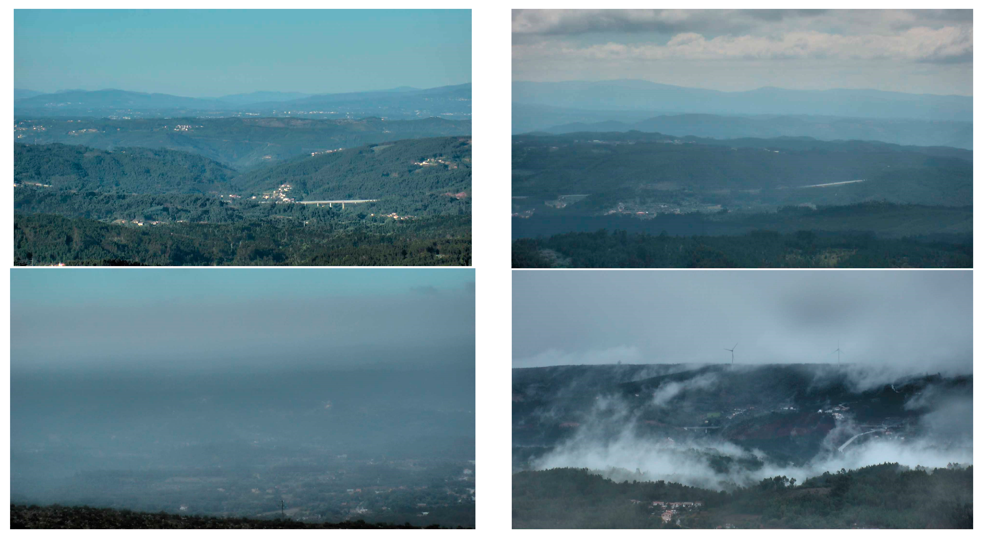
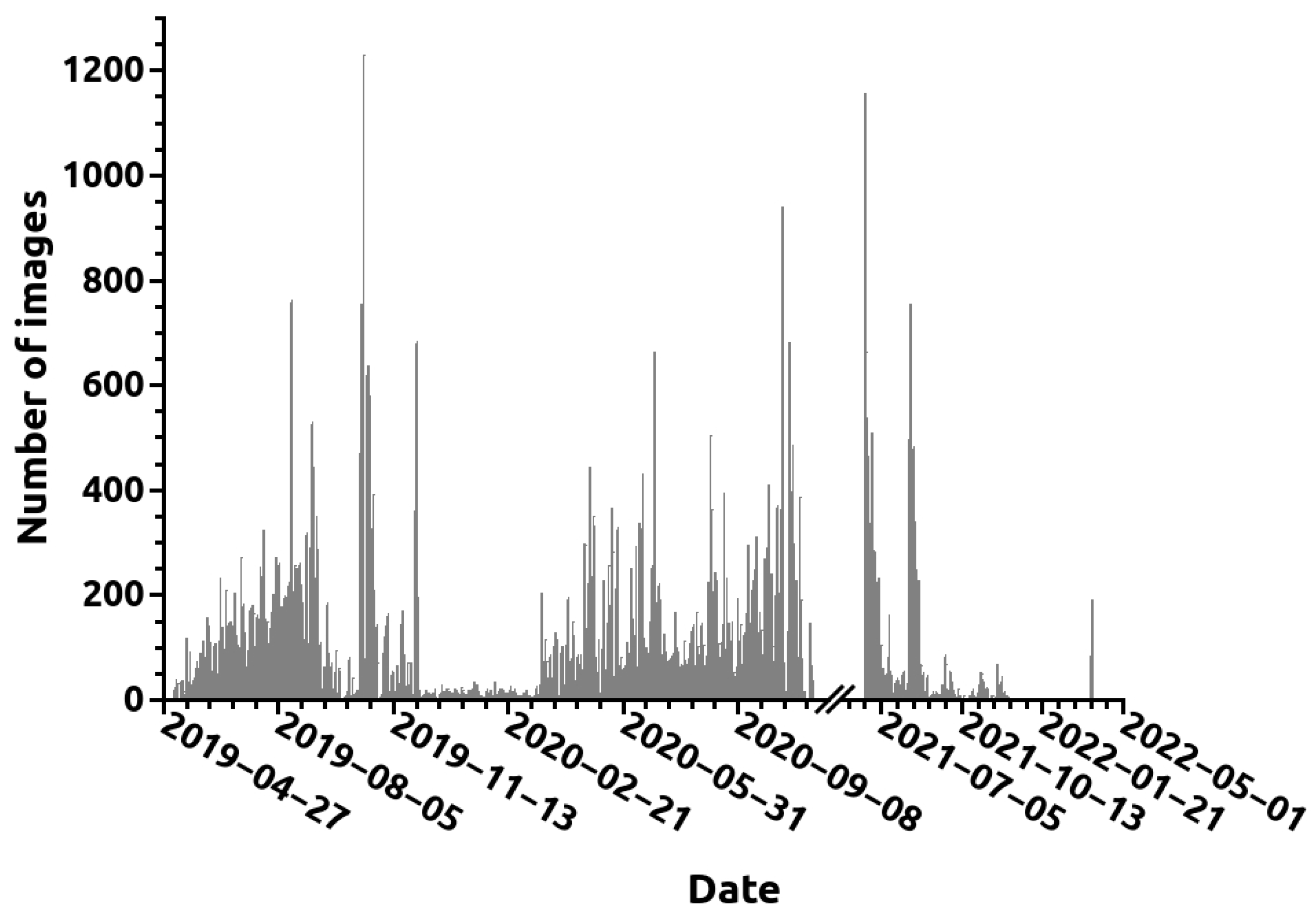
The images employed in the current study were gathered from ten visible cameras installed in surveillance towers in the Leiria region of Portugal. Two examples featuring smoke plumes are shown in Figure 1. The towers are situated between 10 and 60 km from the sea. A total of 26,204 and 51,075 images with and without smoke, respectively, were captured across 361 and 722 different days of the year, for a total of 724 days, since there are images of both types on many days. The cameras’ rotational capability enabled the capture of images from 253 and 271 different viewing directions for smoke and non-smoke images, respectively, culminating in 273 different view directions. The dataset contains images from both hilly and relatively flat regions on days that were either sunny or cloudy. Due to its proximity to the sea, the viewing area is frequently affected by morning fog. Figure 2 depicts the typical images for different cloud coverage and visibility conditions. We have calculated from a 1000 image sampling that the dataset contains approximately 41%, 43%, 9%, and 7% of images with clear sky, clouds, fog/bad visibility, and low clouds, respectively. The images were collected between 6 May 2019 and 24 March 2022. The number of images collected per day during this period is depicted in Figure 3. The dataset was divided into images for training, validation, and testing. The three sets contained 15,655, 5598, and 4951 images with smoke plumes, respectively, and 27,001, 12,002, and 12,072 without. The smoke plume positions in the images were annotated, resulting in a total of 38,170 annotations, as many images contain multiple smoke plumes. The annotations consist of a rectangle that includes the smoke plume. A histogram of the percentage of the image area occupied by every annotation rectangle is given in Figure 4. Most annotations are small, with 88% occupying less than 5% of the image area. The median of the image area occupied is 0.88%.

Figure 1.
Examples of images with smoke plumes in flat (a) and hilly (b) terrain.
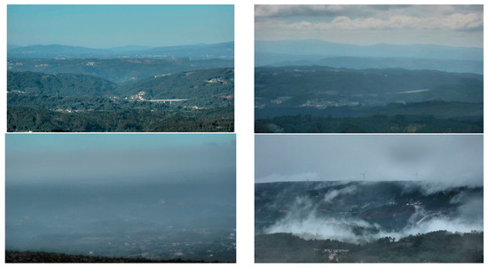
Figure 2.
Representative images for different cloud coverage and visibility conditions. From left to right and top to bottom: clear sky, clouds, fog/bad visibility, and low clouds.

Figure 3.
Number of dataset images collected per calendar day.
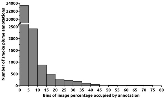
Figure 4.
Histogram of the percentage of each image area covered by a smoke plume annotation. The first bin contains 88% of all annotations.
2.2. EfficientNet
EfficientNets [21], invented in 2019, are an important breakthrough in neural network design. They aim to have a more compact and efficient structure than their predecessors. The main innovation is their scaling approach. EfficientNets pioneered the concept of compound scaling, which simultaneously optimises three network structural features—depth, width, and resolution—in relation to each other. To perform this scaling, one must refine three parameters α, β, and γ through a grid search that allows one to calculate the structural features. The original article tells us that optimal values for α, β, and γ are 1.2, 1.1, and 1.15 for B0, respectively. The architecture of the initial model, EfficientNet-B0, was determined by a selection process using multi-objective neural architecture exploration, aiming to balance accuracy and computational efficiency measured in floating-point operations per second (FLOPS). EfficientNet uses mobile inverted bottleneck (MBConv) blocks [25] augmented with squeeze-and-excitation mechanisms. These blocks employ a series of convolutions to adjust channel numbers and a residual connection. The squeeze-and-excitation technique attributes various weights to different channels, adapting the values during learning to enhance the network’s ability to analyse information efficiently. EfficientNet-B1 through EfficientNet-B7 are built from EfficientNet-B0. Using an exponent ϕ of α, β, and γ, one can calculate the depth, width, and resolution for each new network type from B1 to B7. The ϕ value is related to the value after the “B”. This method ensures balanced growth in all network dimensions without quickly saturating accuracy. As B increases, so does the network complexity, so the number of FLOPS increases by 2ϕ.
2.3. Mosaic-Style Output
The EfficientNets were created to have an output dimensionality equal to 49, corresponding to a 7 × 7 mosaic that equally divides the image. The objective of the mosaic is to allow EfficientNet to detect and localise smoke plumes when EfficientNets are usually employed only for detection. This solution was tested in a previous study with promising results [17]. Adopting a 7 × 7 window allows for accurate detection of the smoke plume region while maintaining reasonable calculation times. In this method, the neural network is trained on a mosaic to assign the value “one” to any mosaic rectangles that overlap with the annotation of a smoke plume in an image. The output is zero when there is no overlap. This method is different from analysing image snippets because the value for each mosaic element is determined using the whole image. The mosaic rectangle is considered to have a value of one and contain smoke when the neural network output is larger than a user-defined detection threshold.
2.4. Evaluation with Receiver Operating Characteristic (ROC) Curves
The results were evaluated using the partial area under the receiver operating characteristic curve (pAUROC). This method involves calculating the receiver operating characteristic (ROC) curve, which maps the true detection percentages versus the false positive percentages. The term “partial” in pAUROC indicates that only a part of the curve is employed for the area determination. In the present case, only the false positive region between 0% and 5% is used because we are interested in ensuring that the choice of the models emphasises the small percentages of false positives. If the whole AUROC is employed, this parameter could lead to optimisation by achieving an elevated true detection percentage in the high false positive region. Such false positive percentages, however, are irrelevant for use in a forest fire detection system. At the same time, this whole AUROC approach might yield an inferior pAUROC compared to a curve based specifically on pAUROC due to reduced true positive percentages within the critically relevant range of low false positive percentages. With pAUROC, we ensure that large true detection percentages are reached for the smallest possible false positive percentages. The “accurate” true detection percentages were calculated using rectification based on GradCAM [26], ensuring that only the detections where the neural network’s “attention” focuses on the annotated smoke plume are considered true detections. This approach was already used in a previous article [17].
2.5. Neural Network Hyperparameter Optimisation
Hyperopt [27], version 0.2.4, is utilised to optimise learning rate, batch size, kernel regularisation, dropout value, and the number of neurons in the fully connected network on the EfficientNets top. Since the training algorithm employed is Nadam [28], it also optimises the two beta values. Hyperopt implements a Bayesian approach called sequential model-based global optimisation (SMBO) [29], which minimises the number of fitness function evaluations to find the most promising hyperparameter values considering previous fitness assessments. This fitness is the pAUROC for each neural network created in the present work. Unlike grid search, which tests all hyperparameter combinations, and random searches, where prior assessments with certain hyperparameters do not influence the selection of new hyperparameters to be tested, Hyperopt offers a more efficient approach.
We ran ten trials to optimise the hyperparameters for each EfficientNet type tested. The maximum number of training epochs was forty, and early stopping ensured good generalisation. The training ended when the pAUROC did not improve after seven epochs. The loss function was binary cross-entropy. Calculations were performed with an image size of 349 × 620 pixels and an augmentation of twice the number of real training images. These values led to good results in Fernandes et al. [17]. The training incorporated transfer learning, meaning each neural network developed for the current application was previously trained on the Imagenet [30] problem. The neural network training was performed with Keras 2.1 [31]. Hyperopt optimised the parameter values of the neural network structure and Nadam training algorithm from the intervals and sets shown in Table 1. Each parameter’s impact on results is not observable to the researcher as it depends on the Hyperopt model.

Table 1.
Neural network structure and training algorithm parameter values optimised with Hyperopt.
3. Results
Table 2 presents the results of an experiment to determine the best type of model for forest fire detection with our dataset. It compares EfficientNets with InceptionV3 and MobileNetV2, which have demonstrated good results in previous works by Fernandes et al., 2022 [17], Govil et al. [23], and Gonçalves et al. [24]. The parameter used for comparison was pAUROC, calculated for false alarms between 0% and 5%; as such, the optimal value would be five in this situation. These experiments were performed without mosaic because that is usually how these algorithms are employed. EfficientNet B2 is the clear winner with a pAUROC of 4.64, followed by InceptionV3 and MobileNetV2 with 4.53 and 4.35, respectively.

Table 2.
Comparison of various model types in terms of pAUROC, without mosaic.
Table 3 presents the outcomes of two distinct experiments using mosaic-style output. The first one comprises the classifiers with indexes from one to four and aims to determine the best type of EfficientNet to adopt. The work consisted of training EfficientNet B0 to B3 to understand which provided the best pAUROC calculated for false alarms between 0% and 5%. EfficientNet B4 and higher were not tested since pAUROC values declined after B1. This trend aligns with expectations, as the larger the networks are, the more data they need to be trained. The training set for this first experiment consisted of 15,000 images containing smoke plumes and 27,000 without smoke plumes. For the classifiers with indexes one to four, the best pAUROC, 4.60, is obtained for case number two, corresponding to an EfficientNet B1. For EfficientNets B0, B2, and B3, the pAUROC values were 4.55, 4.57, and 4.54. It is interesting to notice that the differences in these values are not very large.

Table 3.
Results for the various EfficientNet created with mosaic-style output. Classifier number three, in bold, is the best considering pAUROC, true positives, and false positives. Classifier number two, in italics, has the best pAUROC but inadequate true and false positives. The “T” represents the decision threshold.
The issue with classifier number two lies in its true positive percentage of only 61.9% at a decision threshold of 0.5, a performance significantly lower than one would like for an automatic detection system. The decision threshold is applied to the neural network output values between zero and one; it is the value after which an image is deemed to contain smoke. The false positive percentage is small for the 0.5 threshold, namely 0.142%, which indicates that it might be possible to reduce the threshold to obtain a better true positive percentage and still have an acceptable false positive percentage. However, it does not seem reasonable due to reliability risks. The reason is that for classifiers, it is advisable to have most of the smoke images with values close to one and most images without smoke with values close to zero.
Given this, we decided to look for another classifier, and number three, with the second-best pAUROC, 4.57, emerged as a promising candidate. The true positives of this classifier, for a 0.5 threshold, are 95.4% versus 61.9% of classifier number two, which provides better assurance of good separation between the images with and without smoke. In fact, for a threshold of 0.9, classifier three has a true positive percentage of 87.4%, in stark contrast to the mere 6.38% of classifier number two. Conversely, for false positives, with a 0.1 threshold, classifier number three has 3.47%, and classifier number two has 2.24%. From both true and false positive values, one can infer a much better separation of the images from the two classes regarding neural network output values with classifier number three. For classifier number three, the true positive percentages were 96.9%, 95.4%, and 87.4% for decision thresholds of 0.1, 0.5, and 0.9, respectively. The false-positive percentages were 3.47%, 1.91%, and 0.867%. The precision in the validation set and the 0.9 decision threshold is 97.9%, meaning that only 2.1% of the alarms are false positives. Keeping the percentage of false positives relative to all alarms small is essential so the operator continues paying attention to the alarms.
The pAUROC value of 4.57 for classifier number three, an EfficientNet B2 with mosaic, is slightly smaller than the 4.64 obtained for the same type of neural network without mosaic from Table 2. The slight reduction in pAUROC is, in our opinion, fully compensated by the possibility of locating the smoke plumes. Classifier number three had one hidden layer in the fully connected head of the neural network, comprising 500 neurons and a dropout value of 2.42 × 10⁻³, the learning rate was 1.33 × 10⁻⁵, and the batch size was 32. For Nadam, the β1 and β2 values were 0.901 and 0.981, respectively. The classifier, post-training, takes approximately 14 ms of GPU time on a GeForce RTX 2080 Ti, from NVIDIA, USA, to classify each image. To the GPU time, one must add no more than 50 ms, depending on the computer CPU and disk, to read the image from the disk and redimension it to the neural network input size. Given these times, the whole process is fast enough for real-life monitoring.
The second experiment detailed in Table 3 assesses the performance of classifiers with indexes three, five, and six. For the best EfficientNet type from the first experiment, namely B2, it was tested whether classification percentages are improved when using a more balanced dataset regarding images with and without smoke. With this in mind, two other training sets composed of 15,000 images with smoke plumes but with 15,000 or 21,000 images without plumes were employed in the training of classifiers five and six. The validation and test sets remained unchanged. The pAUROC values obtained for classifiers three, five, and six are 4.57, 4.50, and 4.47, respectively. This sequence reveals a declining trend for this evaluation parameter as the number of images without a smoke plume decreases in the training data. This result suggests that a slightly unbalanced dataset might be helpful when trying to obtain an extremely small percentage of false positives. It is interesting to notice that classifiers five and six present worse pAUROC than the remaining classifiers, which indicates that changing the number of training samples leads to worse outcomes than changing the neural network type.
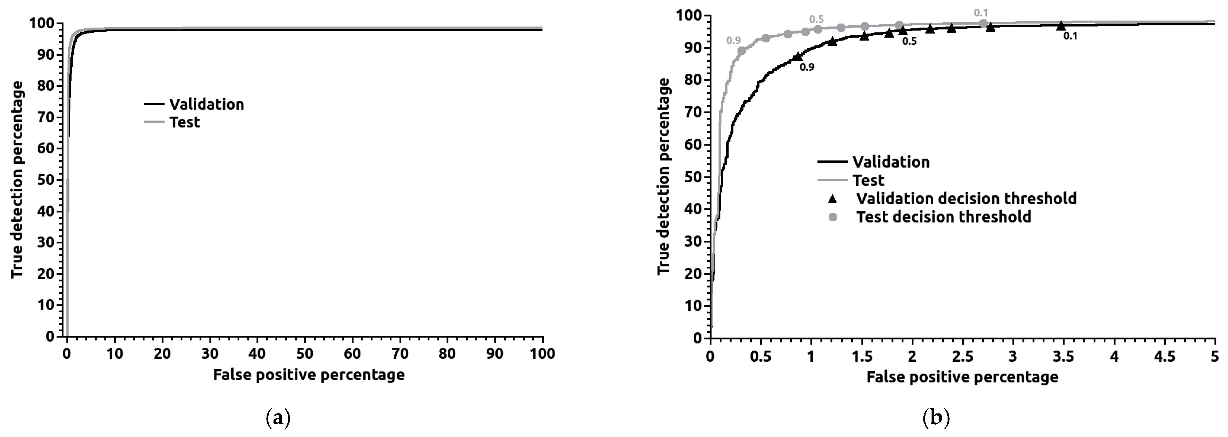
Figure 5 depicts the validation ROC curve for classifier 3. The entire curve is presented on the left (a), while the right image (b) is a detail for false positive percentages smaller than 5%. The right image contains the decision thresholds over the curve. The ROC curves show how robust the algorithm is, regardless of the decision threshold chosen. The figure shows that the validation curve is close to the top left corner of the axis, corresponding to 100% of true detection and 0% of false positives. This point is achievable only with a perfect classifier. The validation curve crosses the 1% of false positives for a decision threshold between 0.8 and 0.9, and at a true detection percentage of 87.4%, the true detection percentages decrease rapidly after the 0.9 threshold.

Figure 5.
Receiver operating characteristic (ROC) curves for classifier number 3 in Table 3. The complete curve is presented on the left (a), whereas a detailed view for false positives below 5% is on the right (b). The values over the curves are the decision threshold values.
Regarding the test results for the decision threshold of 0.9, one obtained a true detection percentage of 89.2% with false positives of 0.306%. The test ROC curve is also shown in Figure 5. The result of the test represents a difference/improvement compared to the validation values of 1.80 percentage points and 0.561 percentage points, respectively. The difference is easily visible in the ROC curves in Figure 5, since the test curve is closer to the optimal point. In the test ROC curve, the drop in true detection percentages after the 0.9 value of the decision threshold is sharper than for the validation curve. The precision in the test for the 0.9 threshold is 99.2%. The accuracy, defined as the proportion of correctly classified images, both with and without smoke, out of the total number of images, is 96.6%.
The test results surpass those obtained in validation, which is unusual. The most typical is to have better results in the validation set because the hyperparameters were tuned specifically for this set. However, it is not impossible to have better results in the test set because, in the present application, it is hard to be sure that the images in the validation and test sets present the same degree of difficulty concerning smoke plume identification when given to the classifier. Nevertheless, the discrepancy between validation and test outcomes is not significant enough for us to question the classifier’s quality.
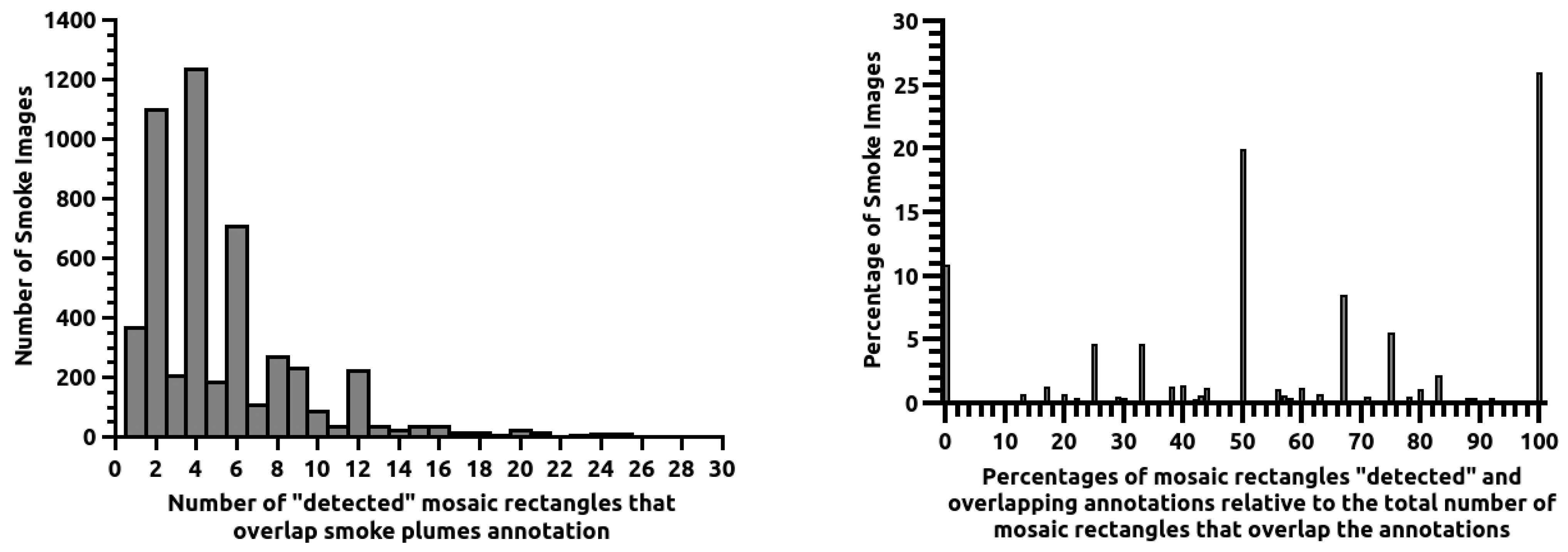
We detect smoke regions using the mosaic-shaped output of classifiers and analyse how closely the classifiers’ responses match the desired mosaic encoding the annotation. When the mosaic rectangles have a classifier output larger than the defined detection threshold, we say that these rectangles were “detected” because the classifier indicates that they probably contain a smoke plume. Figure 6 shows, on the left, the distribution of images with a certain number of mosaic rectangles “detected” and overlapping the smoke plume annotations; the right image shows the distribution of images with different percentages of the mosaic rectangles “detected” and overlapping annotations relative to the total number of mosaic rectangles that overlap the annotation. Both distributions are for data from the test set. In Figure 6, on the left, one may see that the number of mosaic rectangles overlapping with annotations is most frequent even instead of odd. This is due to the number of mosaic rectangles for each annotation being a product of two integer values, one for each of the xx and yy dimensions, and the product of two integers is only an odd number in 25% of the cases when two odd numbers are multiplied. The first detail that stands out in the right image of Figure 6 is that the percentage of images with 100% mosaic rectangles “detected” by our best neural network is far from 100%; it is 25.9%. The second largest peak in the distribution, corresponding to 19.8%, occurs for 50% of rectangles “detected”, and 70.1% of all smoke images have 50% or more of the desired mosaic rectangles correctly “detected”. The peak at 50% is, in approximately 80% of the cases, due to images with two or four mosaic rectangles overlapping an annotation where one or two rectangles are not “detected”. Despite this, a small percentage of rectangles detected still guide the system operator’s attention to the presence of a smoke plume.
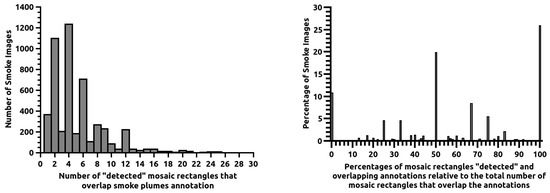
Figure 6.
On the left, the distribution of images with a certain number of the 7 × 7 mosaic rectangles “detected” and overlapping the smoke plume annotation. The right picture depicts the distribution of images with various percentages of mosaic rectangles “detected” and overlapping annotations relative to the total number of mosaic rectangles that overlap the annotations. Both distributions are for images from the test set.
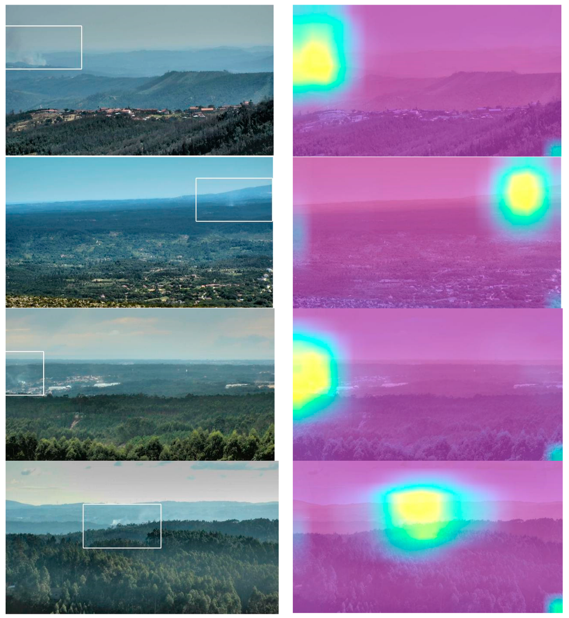
Figure 7 depicts various examples of smoke plume detections signalled with white rectangles. The right column displays GradCam maps with yellow spots indicating the regions where the neural network attention is concentrated. A good match exists between the large attention regions and the smoke plume position. The white rectangles correspond to the union of the areas of the mosaic rectangles with neural network outputs larger than the decision threshold.
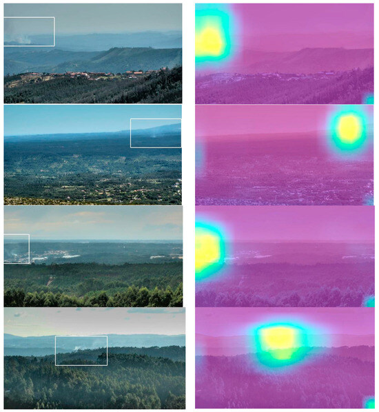
Figure 7.
Illustrative instances of smoke plume detections. The (left column) shows the white rectangle indicating smoke plume detections. The (right column) presents the corresponding GradCAM image with the yellow spot marking the neural network’s attention region.
4. Discussion
4.1. Comparison to Previous Works
Regarding prior research, the test set results have shown significant improvement, moving from 80.4% of true positives and 1.13% of false positives in EfficientDet by Fernandes et al., 2023 [18], to 89.2% and 0.306%, respectively. The results indicate an enhancement of 8.8 percentage points in true detection while decreasing the false positive percentage by more than three-fold. Despite now utilising EfficientNet, it exhibits smoke plume location ability due to the mosaic-style output. However, the mosaic squares are fixed for EfficientNet, while in EfficientDet, the location window positioning and size are highly flexible, making the former less precise regarding location. Still, the improvement in classification efficiency seems to compensate. Fernandes et al., 2022 [17], employed a 3 × 3 mosaic with good results, but that work did not clarify if a more detailed grid would yield good results. The present work resolves this uncertainty by creating efficient models with a 7 × 7 mosaic.
Compared to Fernandes et al., 2022 [17], whose best model is an EfficientNet B0, the larger dataset seems beneficial by facilitating better generalisation of more complex EfficientNets such as B2. In addition, a larger, high-quality dataset usually leads to better results due to a more realistic foundation for learning and adjusting hyperparameters, followed by a more rigorous test of the model’s generalisation ability. Overall, a larger dataset means a more reliable model is developed.
Regarding works from other authors, Frizzi et al. [20] and Yin et al. [19] reported 96.37% and 96.6% of true positives and 1.2% and 0.6% of false positives, respectively. These values are among the best reported for outdoor smoke detection. It is relevant to stress that a direct comparison between our results and theirs cannot be made because the datasets are different; however, one can use their result as an indicative guide. For 0.6% of false positives, we obtained 93.5% of true positives in the test set, indicating that our models are competitive. Our results are even more compelling given the larger size of our datasets, which enhances the results’ reliability. Yin et al., with the lowest false positive percentage, tested their models with 1240 and 1648 images with and without smoke, respectively, while we employed 4951 and 12,072. In addition, their images are not similar to what one would expect while doing surveillance of landscapes for wildfire detection. In Frizzi et al. [20], the images depict some close-range fires and burning buildings, both with visible flames; in Yin et al. [19], the smoke images contain only smoke, without any visible landscape. These characteristics significantly differ from our dataset, which includes landscapes viewed from afar with small smoke plumes. Other works have reported good accuracy, reaching 97.72% by Khan et al. [32], 98.72% by Sathishkumar et al. [33], and 99.53% by Valikhujaev et al. [34]. However, their datasets are formed by a mix of images collected from close-range and large distances [32,34] and even satellite images [33]. This composition makes, once again, their datasets significantly different from ours, so their results are only indicative references for our work, which achieves an accuracy of 96.6%. In addition, Sathishkumar et al., Valikhujaev et al., and Khan et al. use 4800, 16,860, and 36,006 real images, far from our 77,279 images.
Govil et al. [23] use images similar to ours. Their dataset contains more images without smoke but approximately three times fewer images with smoke. A true positive percentage of 86% is provided only for an extremely small dataset with 100 images containing smoke. Their results seem relevant regarding false positives, 0.66 per day per camera, but no true positive percentage is given for the same dataset, preventing an adequate analysis.
Gonçalves et al. [24] also use images similar to ours. They utilise a dataset of 8991 images, smaller than ours and comprising an image selection from a prior algorithm. In their study, using models that incorporate transfer learning, as we do, the smallest reported false positive percentage was 0.4% for a MobileNetV2.
The small number of false positives Govil et al. and Gonçalves et al. obtained for images like ours prompted a comparison of our neural networks, EfficientNets, with Govil et al.’s InceptionV3 and Gonçalves et al.’s MobileNetV2. To this end, the InceptionV3 and the MobileNetV2 were optimised the same way as the EfficientNets and with the same datasets as neural networks with indexes 2 and 3 from Table 3. However, no mosaic was employed in the comparison because Govil et al. and Gonçalves et al. did not use it. The best pAUROC, in the 0% to 5% interval, obtained for InceptionV3 was 4.53, and for MobileNetV2, it was 4.35, which compares to 4.64 from EfficientNet B2. These results show that EfficientNet performs better than InceptionV3 and MobileNetV2 for our data.
4.2. Mosaic-Style Output
As previously mentioned, the mosaic output allows for identifying the smoke plume location. For a mosaic element to be recognised as detection in this study, it must coincide with elements exhibiting neural network output values exceeding the detection threshold and overlap with those marked by a smoke plume annotation. We observed that only 25.9% of the smoke images have all mosaic rectangles overlapping a smoke plume annotation correctly “detected” by the classifier. We believe that two reasons can explain this fact: (1) The rectangular annotation box is inadequate to describe the smoke plumes. This inadequacy comes from many plumes having slightly triangular or circular shapes, which causes the annotations to overlap some mosaic rectangles that do not contain any smoke. (2) The mosaic rectangles are, in some cases, covered by smoke in only a small extension, making detection harder.
In this context, complete detection of all mosaic rectangles overlapping the smoke plume annotation is not crucial. The primary objective of identifying the smoke plume location serves three purposes: (1) To make sure that the classifier focused on the smoke plume when issuing a detection; (2) To help the detection system operator confirm the detection; (3) To allow discarding repeated alarms from a certain location. For these purposes, our location accuracy is sufficient, even though improving it would strengthen the efficacy of the three purposes.
4.3. Class Imbalance
In wildfire detection, the imbalance in data is usual, meaning that during a day of surveillance, one may gather thousands of images, and only in a few days will the images contain smoke plumes. The previous section has given results for situations where the number of training samples without smoke varied from equal to almost twice that of images with smoke. Balancing the various classes in the training set prevents bias towards the better-represented class. An imbalance may lead to suboptimal performance for the less-represented class. This phenomenon happens because, while training with backpropagation, the gradients will be more influenced by the images of the majority class. The classifier may even overlook the less-represented class, consistently outputting the majority class’s desired value. As long as the neural network can learn the data, keeping the data imbalance as close as possible to reality is good because your classifier will know the real-world distributions of the data to classify.
Addressing the challenge of imbalanced datasets is crucial, especially in cases where two classes are disproportionately represented. For example, if one class comprises only 1% of the dataset, even if the classifier always answers that every sample corresponds to the majority class, this “blind” classifier will still be 99% correct. Therefore, when providing results for imbalanced data, one must carefully separate the classification efficiencies of the various classes and use ROC curves to assess the balance between the results of the multiple classes. This is what we have achieved. Our best results are obtained for 15,000 and 27,000 images with and without smoke, respectively. This imbalance is mild; a severe one would have one class representing less than 1% of the dataset. We see that the existing imbalance is positive for obtaining better pAUROC. The current article does not try to address larger imbalances by using more images without smoke for training because none are left after attributing reasonable amounts to the validation and test sets. However, future research should investigate whether more pronounced imbalances could further enhance the results.
4.4. Misdetections (False Negatives) and False Positives
In Figure 8, various instances of misdetections and false positives are presented. The misdetections are depicted in the left column, labelled as (a). In the dataset used, one may discover undetected smoke plumes, large and small, with a ground or sky background and captured under various lighting conditions at different hours of the day. Consequently, no possible reason was found for the created neural networks to disregard some smoke plumes.
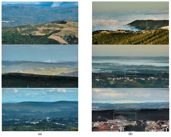
Figure 8.
Examples of images. (a) On the left are smoke plumes of various sizes that were not detected; (b) On the right are cases originating false positives marked with a white rectangle. The two top cases in column (b) are low clouds.
Regarding false positives, in the right column (b), clouds are often a common cause, whether near the ground or higher in the sky. This fact is worrying when the estimate of the images in the dataset with clouds is 50%. The reason for the false positives is that clouds are similar to smoke plumes in both shape and colour. However, most clouds do not trigger false alarms; if they trigger false alarms, obtaining the false positive percentages at the reported levels would be unfeasible. Consequently, what exactly triggers the false positive is unknown. There are also cases where some natural structures, such as trees, can assume a shape that triggers an alarm; please see the bottom right corner image in Figure 8. In other situations, one cannot identify the false positive cause.
4.5. Small Smoke Plumes
Figure 9 presents various images with small smoke plumes. Their location is at the lower left region for (a), at the top left close to the image border for (b), at the lower right corner for (c), and at the centre of the image over the horizon line for (d). Smoke plumes (a), (b), and (c) are discernible due to their contrast, regardless of their small size. The major difficulty in identifying (a) comes from its white colour, which blends with buildings. Plumes (b) and (c) appear on the image’s edge, often missed by observers. Plume (d) is hard to see. For (d), only a spot of bright white immediately over the trees is distinguishable; afterwards, one might see a faint plume rising. The eyes struggle to differentiate it from the background, even knowing it is there. One might think that three out of the four examples are not very hard to spot. Now, one must consider: (1) A surveillance system produces a new image from each tower approximately every four seconds because the cameras are rotating; (2) Each operator may need to watch multiple cameras simultaneously; (3) The image-watching task will continue for hours and then days, with most images, fortunately, having no smoke plume. These characteristics make the surveillance work hard and tedious. Under these conditions, an automated surveillance system becomes a fundamental and welcome aid, as long as it does not produce too many false positives. The necessity of an automatic system does not come primarily from the impossibility of humans finding the plumes, even though it may sometimes be difficult, as in case (d), but predominantly due to the demanding conditions under which the plumes must be found.
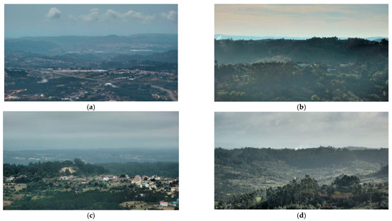
Figure 9.
(a–d) contain various examples of images with small smoke plumes detected by our best neural network. The plume positions are not marked, so the reader tries to find them.
4.6. Validation Versus the Test Results
As seen previously, the test set presents better classification results than the validation set, most probably due to differences in the difficulty of classifying images in both sets. The images were randomly chosen for each dataset, and images from different days can look quite different due to changes in sun exposure caused by the presence or absence of clouds. Visibility can also change due to humidity in the atmosphere and the existence of fog or low clouds. The lack of deep knowledge about the root causes of misdetections and false positives makes it almost impossible to ensure that both validation and test sets have equal degrees of difficulty for classification.
4.7. Deployment Issues
The integration of the proposed technology into existing surveillance systems is straightforward. Regarding software, the neural networks can be run in a separate module that receives one image as input and outputs the window coordinates of the smoke plume. This module is a relatively simple piece of code. The code steps include the following: (1) load the neural network and prepare it for processing; (2) receive an image; (3) convert the image to a format the neural network can process; (4) send the image to the neural network; (5) get the neural network output and convert it as needed; and (6) return to the main code the output in a recognisable format. The image processing can be performed at a control centre that receives all the images from multiple surveillance cameras. The developed neural network can operate on a GPU or even on a CPU, as real-time image classification is not required. Since the surveillance cameras usually rotate to cover 360 degrees, there are a few seconds when the camera moves, during which no images are available for processing.
Regarding operation under various weather conditions, heavy fog or rain can strongly impact visibility and detection. Nevertheless, with rain, there is no fire risk, and fog increases humidity, reducing the fire risk. Cloud cover is consistently an issue because a sky without clouds is not the most usual, even in summer.
5. Conclusions
The present work shows that EfficientNet, outputting a 7 × 7 mosaic to segment the image to be classified, can provide good results in detecting and locating smoke plumes in visible light images from remote cameras. Usually, EfficientNets lack object location abilities, but the mosaic output endows them with this functionality. The results have shown that class imbalance does not necessarily hinder performance, as the most effective neural network was trained with 15,000 and 27,000 images with and without smoke, respectively. Notably, smaller imbalances led to poorer results. In terms of false positives, the clouds seem to be the system’s archenemy due to their strong resemblance to smoke plumes. The causes of misdetections remain elusive, as no distinct characteristic hindering detection has been identified.
Our top-performing classifier achieves a true detection percentage of 89.2% with a notably low false positive percentage of only 0.306%. The best results in the scientific literature for smoke detection, obtained for a dataset different from ours and significantly smaller, are 96.6% true positives and 0.6% false positives. By adjusting our decision threshold to match a 0.6 false positive percentage, we obtain 93.5% of true positives. A strict comparison of values cannot be made with the best results due to the differences in the smoke images. Still, it is relevant to notice the high performance of our EfficientNets in our extensive and realistic dataset. Govil et al. [23] and Gonçalves et al. [24] purpose and image content are similar to those employed here; compared to their InceptionV3 and MobileNetV2, which provided interesting false positive values, our EfficientNets perform better. Regarding the works of Fernandes et al., 2022 [17] and Fernandes et al., 2023 [18], which use a subset of the present work dataset, there are relevant improvements in false positive and true positive percentages.
In future work, we would like to continue increasing the dataset size since this is one of the best ways to enhance results. With the larger dataset, it may also be possible to effectively train larger EfficientNets, such as B4, with an extra boost in performance. The main objective will to enhance the true detection percentages to values well above 90% without worsening the false positive percentage. Other research directions will include testing different neural network architectures and incorporating images from new geographic regions into the dataset. Further development and testing of the mosaic-style output is a must.
Author Contributions
Conceptualisation, A.F., A.U. and P.C.; software, A.F.; investigation, A.F.; resources, P.C.; writing—original draft preparation, A.F.; writing—review and editing, A.F., A.U., and P.C.; project administration, A.F., A.U. and P.C.; funding acquisition, A.F., A.U. and P.C. All authors have read and agreed to the published version of the manuscript.
Funding
This work was supported by project ResNetDetect with the number PCIF/MPG/0051/2018 from “Fundação para a Ciência e a Tecnologia” in Portugal. The project has DOI http://doi.org/10.54499/PCIF/MPG/0051/2018.
Institutional Review Board Statement
Not applicable.
Informed Consent Statement
Not applicable.
Data Availability Statement
The data cannot be made public due to data protection issues.
Conflicts of Interest
The authors declare no conflicts of interest. The funders had no role in the design of the study; in the collection, analyses, or interpretation of data; in the writing of the manuscript; or in the decision to publish the results.
References
- Fire Lookout. Available online: https://firelookout.org/index.html (accessed on 18 December 2023).
- Fernandes, A.M.; Utkin, A.B.; Lavrov, A.V.; Vilar, R.M. Development of Neural Network Committee Machines for Automatic Forest Fire Detection Using Lidar. Pattern Recognit. 2004, 37, 2039–2047. [Google Scholar] [CrossRef]
- Fernandes, A.M.; Utkin, A.B.; Lavrov, A.V.; Vilar, R.M. Design of Committee Machines for Classification of Single-Wavelength Lidar Signals Applied to Early Forest Fire Detection. Pattern Recognit. Lett. 2005, 26, 625–632. [Google Scholar] [CrossRef]
- Dampage, U.; Bandaranayake, L.; Wanasinghe, R.; Kottahachchi, K.; Jayasanka, B. Forest Fire Detection System Using Wireless Sensor Networks and Machine Learning. Sci. Rep. 2022, 12, 46. [Google Scholar] [CrossRef]
- de Almeida, R.V.; Vieira, P. Forest Fire Finder—DOAS Application to Long-Range Forest FIre Detection. Atmos. Meas. Tech. 2017, 10, 2299–2311. [Google Scholar] [CrossRef]
- Barmpoutis, P.; Papaioannou, P.; Dimitropoulos, K.; Grammalidis, N. A Review on Early Forest Fire Detection Systems Using Optical Remote Sensing. Sensors 2020, 20, 6442. [Google Scholar] [CrossRef]
- Bouguettaya, A.; Zarzour, H.; Taberkit, A.M.; Kechida, A. A Review on Early Wildfire Detection from Unmanned Aerial Vehicles Using Deep Learning-Based Computer Vision Algorithms. Signal Process. 2022, 190, 108309. [Google Scholar] [CrossRef]
- Signalert. Available online: http://www.signalert.net/en/ (accessed on 18 December 2023).
- Baek, J.; Alhindi, T.J.; Jeong, Y.-S.; Jeong, M.K.; Seo, S.; Kang, J.; Shim, W.; Heo, Y. A Wavelet-Based Real-Time Fire Detection Algorithm with Multi-Modeling Framework. Expert. Syst. Appl. 2023, 233, 120940. [Google Scholar] [CrossRef]
- Zhang, T.; Wang, Z.; Zeng, Y.; Wu, X.; Huang, X.; Xiao, F. Building Artificial-Intelligence Digital Fire (AID-Fire) System: A Real-Scale Demonstration. J. Build. Eng. 2022, 62, 105363. [Google Scholar] [CrossRef]
- IQ Firewatch. Available online: https://www.iq-firewatch.com/ (accessed on 18 December 2023).
- Alkhatib, A.A.A. A Review on Forest Fire Detection Techniques. Int. J. Distrib. Sens. Netw. 2014, 10, 597368. [Google Scholar] [CrossRef]
- SmokeD. Available online: https://smokedsystem.com/ (accessed on 18 December 2023).
- HPWREN. Available online: https://hpwren.ucsd.edu/ (accessed on 18 December 2023).
- CICLOPE. Available online: https://www.ciclope.com.pt/ (accessed on 18 December 2023).
- Peng, Y.; Wang, Y. Automatic Wildfire Monitoring System Based on Deep Learning. Eur. J. Remote Sens. 2022, 55, 551–567. [Google Scholar] [CrossRef]
- Fernandes, A.M.; Utkin, A.B.; Chaves, P. Automatic Early Detection of Wildfire Smoke With Visible Light Cameras Using Deep Learning and Visual Explanation. IEEE Access 2022, 10, 12814–12828. [Google Scholar] [CrossRef]
- Fernandes, A.M.; Utkin, A.B.; Chaves, P. Automatic Early Detection of Wildfire Smoke with Visible-Light Cameras and EfficientDet. J. Fire Sci. 2023, 41, 122–135. [Google Scholar] [CrossRef]
- Yin, Z.; Wan, B.; Yuan, F.; Xia, X.; Shi, J. A Deep Normalisation and Convolutional Neural Network for Image Smoke Detection. IEEE Access 2017, 5, 18429–18438. [Google Scholar] [CrossRef]
- Frizzi, S.; Kaabi, R.; Bouchouicha, M.; Ginoux, J.-M.; Moreau, E.; Fnaiech, F. Convolutional Neural Network for Video Fire and Smoke Detection. In Proceedings of the IECON 2016—42nd Annual Conference of the IEEE Industrial Electronics Society, Florence, Italy, 23–26 October 2016; pp. 877–882. [Google Scholar]
- Tan, M.; Le, Q.V. EfficientNet: Rethinking Model Scaling for Convolutional Neural Networks. arXiv 2020, arXiv:1905.11946. [Google Scholar]
- Tan, M.; Pang, R.; Le, Q.V. EfficientDet: Scalable and Efficient Object Detection. arXiv 2020, arXiv:1911.09070. [Google Scholar]
- Govil, K.; Welch, M.L.; Ball, J.T.; Pennypacker, C.R. Preliminary Results from a Wildfire Detection System Using Deep Learning on Remote Camera Images. Remote Sens. 2020, 12, 166. [Google Scholar] [CrossRef]
- Gonçalves, A.M.; Brandão, T.; Ferreira, J.C. Wildfire Detection With Deep Learning—A Case Study for the CICLOPE Project. IEEE Access 2024, 12, 82095–82110. [Google Scholar] [CrossRef]
- Sandler, M.; Howard, A.; Zhu, M.; Zhmoginov, A.; Chen, L.-C. MobileNetV2: Inverted Residuals and Linear Bottlenecks. In Proceedings of the 2018 IEEE/CVF Conference on Computer Vision and Pattern Recognition, Salt Lake City, UT, USA, 18–23 June 2018; pp. 4510–4520. [Google Scholar]
- Selvaraju, R.R.; Cogswell, M.; Das, A.; Vedantam, R.; Parikh, D.; Batra, D. Grad-CAM: Visual Explanations from Deep Networks via Gradient-Based Localization. Int. J. Comput. Vis. 2020, 128, 336–359. [Google Scholar] [CrossRef]
- Bergstra, J.; Komer, B.; Eliasmith, C.; Yamins, D.; Cox, D.D. Hyperopt: A Python Library for Model Selection and Hyperparameter Optimization. Comput. Sci. Discov. 2015, 8, 014008. [Google Scholar] [CrossRef]
- Dozat, T. Incorporating Nesterov Momentum into ADAM. In Proceedings of the ICLR 2016 Workshop, San Juan, Puerto Rico, 2–4 May 2016. [Google Scholar]
- Bergstra, J.; Bardenet, R.; Bengio, Y.; Kegl, B. Algorithms for Hyper-Parameter Optimization. In Proceedings of the 24th International Conference on Neural Information Processing Systems, Granada, Spain, 12–15 December 2011; pp. 2546–2554. [Google Scholar]
- Russakovsky, O.; Deng, J.; Su, H.; Krause, J.; Satheesh, S.; Ma, S.; Huang, Z.; Karpathy, A.; Khosla, A.; Bernstein, M.; et al. ImageNet Large Scale Visual Recognition Challenge. Int. J. Comput. Vis. 2015, 115, 211–252. [Google Scholar] [CrossRef]
- Keras. Available online: https://keras.io/ (accessed on 18 December 2023).
- Khan, S.; Muhammad, K.; Mumtaz, S.; Baik, S.W.; De Albuquerque, V.H.C. Energy-Efficient Deep CNN for Smoke Detection in Foggy IoT Environment. IEEE Internet Things J. 2019, 6, 9237–9245. [Google Scholar] [CrossRef]
- Sathishkumar, V.E.; Cho, J.; Subramanian, M.; Naren, O.S. Forest Fire and Smoke Detection Using Deep Learning-Based Learning without Forgetting. Fire Ecol. 2023, 19, 9. [Google Scholar] [CrossRef]
- Valikhujaev, Y.; Abdusalomov, A.; Cho, Y.I. Automatic Fire and Smoke Detection Method for Surveillance Systems Based on Dilated CNNs. Atmosphere 2020, 11, 1241. [Google Scholar] [CrossRef]
Disclaimer/Publisher’s Note: The statements, opinions and data contained in all publications are solely those of the individual author(s) and contributor(s) and not of MDPI and/or the editor(s). MDPI and/or the editor(s) disclaim responsibility for any injury to people or property resulting from any ideas, methods, instructions or products referred to in the content. |
© 2024 by the authors. Licensee MDPI, Basel, Switzerland. This article is an open access article distributed under the terms and conditions of the Creative Commons Attribution (CC BY) license (https://creativecommons.org/licenses/by/4.0/).


