Article

Numerical Simulation and Consequence Analysis of Full-Scale Jet Fires for Pipelines Transporting Pure Hydrogen or Hydrogen Blended with Natural Gas

1
College of Safety Science and Engineering, Nanjing Tech University, Nanjing 211816, China
2
Institute of Fire Science and Engineering, Nanjing Tech University, Nanjing 211816, China
*
Authors to whom correspondence should be addressed.
Fire 2024, 7(6), 180; https://doi.org/10.3390/fire7060180
Submission received: 12 April 2024 / Revised: 8 May 2024 / Accepted: 19 May 2024 / Published: 24 May 2024
(This article belongs to the Special Issue State-of-the-Art on Hydrogen Combustion)

Abstract

:
The use of existing natural gas pipelines for the transport of hydrogen/natural gas mixtures can achieve large-scale, long-distance and low-cost hydrogen transportation. A jet fire induced by the leakage of high-pressure pure hydrogen and hydrogen-blended natural gas pipelines may pose a severe threat to life and property. Based on the Abel–Nobel equation of state and a notional nozzle model, an equivalent pipe leakage model is established to simulate high-pressure pipeline gas leakage jet fire accidents. Large-scale high-pressure hydrogen and natural gas/hydrogen mixture jet fires are simulated, showing the jet impingement process and obtaining an accurate and effective simulation framework. This framework is validated by comparing the simulated and experimental measured results of flame height, flame appearance and thermal radiation. Several combustion models are compared, and the simulated data show that the non-premixed chemical equilibrium combustion model is superior to other combustion models. The influence of the pipe pressure and the hydrogen blending ratio on the consequences of natural gas/hydrogen mixture pipeline leakage jet fire accidents is explored. It is found that when the hydrogen blending ratio is lower than 22%, the increase in the hydrogen blending ratio has little effect on the decrease in the thermal radiation hazard distance.

1. Introduction

The past decades have witnessed significant growth in our awareness of climate change and energy scarcity. Thus, pursuing cleaner and more sustainable energy sources to gradually replace traditional fossil fuels is rated as a top priority for development [1,2]. One such potential energy source is hydrogen, which is a carbon-free eco-friendly gas with a high energy content of 120 MJ/kg [3], has been regarded as an ideal choice for energy transformation and is becoming increasingly popular worldwide [4,5]. Referring to the IEA’s recent report “Global Hydrogen Review 2022”, the global hydrogen demand in 2021 was 94 million tons, with projections that this will increase by more than 20% by 2030 [6]. It is anticipated that hydrogen will be produced in large quantities, and the challenges of hydrogen transportation and storage have been identified as significant barriers for its large-scale application. At present, the most promising focus has been on blending hydrogen into existing natural gas pipelines to benefit from its large scale, low cost and application for long-distance transportation [7,8]. However, due to the mixing of hydrogen, hydrogen embrittlement in metallic pipes, its wide flammability limit and its high combustion speed, mixed transport poses safety risks [9]. Among all relevant accidents, the worst-case scenario is a jet fire caused by accidental pipeline leakage [10,11], which has been an ongoing concern in risk assessments of fire safety and protection in the process industries. Therefore, it is necessary and urgent to study the resulting jet fire hazards after the leakage of high-pressure pure hydrogen and hydrogen-blended natural gas pipelines.
Research has been conducted with experimental tests on the hazards created by jet fires involving pure hydrogen or natural gas/hydrogen mixtures. Schefer et al. [12] investigated the flame length and radiant heat flux of hydrogen jet fires originating from high-pressure tanks up to 41.3 MPa and with a 0.508 cm jet diameter, as well as the storage pressure and temperature variations during a tank blowdown. The maximum flame length was 11.3 m. Acton et al. [13] conducted two large-scale hydrogen pipeline jet fire experiments. At an initial pressure of 60 bar, the jet flowed out of a pipe rupture with a 0.1524 m diameter. They found that the soil used for pipeline backfill has less influence on the thermal radiation levels of jet fires up to 100 m in height than the weather conditions. Proust et al. [14] measured the mass flow rate, jet flame length and radiant heat flux during the blowdown process of a 90 MPa hydrogen tank through orifices ranging from one to three mm in diameter, and the Abel–Nobel equation of state (EOS) was used to make better predictions of the hydrogen density variation. The maximum flame length was no more than seven m. Lowesmith and Hankinson [15,16] tested large-scale high-pressure jet fires induced by hydrogen-blended natural gas pipeline leaks. Valuable data were obtained which can assist in evaluating fire hazards following such pipeline failures. Wu et al. [17] carried out experiments on the effects of the addition of hydrogen to methane on the emission and heat transfer characteristics of laminar diffusion flames. The jet formed a flame with a maximum length of no more than 350 mm through a 7.6 mm diameter nozzle. They found that the increase in hydrogen addition increased the flame temperature and the total flame heat flux, but decreased the flame length. Hooker et al. [18] carried out experiments on the fire behavior of hydrogen jets in a passively ventilated enclosure. They found that the behavior of the hydrogen jet fires was affected by the release rate of hydrogen, the area of the vent and the thermal performance of the shell. Xiao et al. [19] carried out a hydrogen jet fire experiment inside a chamber and found that the heat and mass transfer to the chamber walls significantly affected the dynamics of the hydrogen jet fire. In their experiment, the diameter of the hydrogen nozzle was 0.005 m, and the size of the test chamber was 0.98 m long, 0.96 m wide and 1 m high. Tang et al. [20] carried out hydrogen jet fire experiments with diverse fuel flow rates, nozzle diameters and inclination angles under the action of a water curtain, and a correlation was proposed for the flame extension length based on a new dimensionless heat release rate and the air entrainment coefficient. In their experiment, circular nozzles with diameters of 5 mm, 10 mm and 15 mm were used, and the maximum flame extension length did not exceed 20 cm. Zhao et al. [21] tested small-scale hydrogen/methane jet fires, and the effects of the hydrogen blending ratio, nozzle diameter and heat release rate on the flame geometrical characteristics were explored. In their experiment, the fuel flowed out from circular nozzles with different diameters of three mm and five mm, and the flame height did not exceed 650 mm. The previous works obtained the flame morphological characteristics and thermal radiation hazards via experiments, which helped to assess the hazard of a jet fire induced by the leakage of pure hydrogen and natural gas/hydrogen mixtures. However, large-scale high-pressure jet fire experiments resulting from the leakage of hydrogen or hydrogen-blended natural gas pipelines usually encounter difficulties in many aspects, e.g., safety risks, economic costs and operational problems.
Some scholars have used theoretical models to evaluate leakages and resulting jet fire hazards. The gas leakage behavior can be physically described using a gas equation of state (EOS) and an isentropic process. Previous models based on the ideal gas EOS generally relate to the case of low-pressure leakage, but high-pressure gas exhibits a highly non-ideal behavior, and a more complicated application of a real gas EOS is required [22,23]. A methodology for the risk assessment of gas transmission pipelines was proposed in the PIPESAFE package [24]. This includes a range of mathematical models, such as a pipeline outflow model, a crater source model and an immediate ignition model, to perform a consequence analysis of a ruptured pipeline. Liu et al. [25] and Zhou et al. [26] established an integrated model which includes a high-pressure leakage process model, a notional nozzle model and a flame size model. The integrated model was shown to predict the flame length well. Zhou et al. [27] built a theoretical framework to predict the full-scale jet fire hazards induced by the leakage of hydrogen and a mixture with 22.3% hydrogen and 77.7% natural gas. These works have mainly focused on pure natural gas or hydrogen leakages and their combustion behaviors, and great advances have been made. However, the jet fire hazards of hydrogen blended with natural gas are not sufficiently explored. In addition, the current theoretical calculation methods are very complex for practical use, as there are operational difficulties and coupling complexities among various sub-models.
With the development of computer technology and computational fluid dynamics (CFD) techniques, CFD numerical simulations have also been used to investigate the consequences of jet fires [28,29]. The CFD software tools that have been used include ANSYS Fluent [30,31], FLACS [32], HyRAM [33] and FDS [34]. Consalvi and Nmira [35] simulated small-scale hydrogen and methane jet fires and large-scale under-expanded hydrogen jet fires with an in-house CFD code. Shan et al. [36] constructed an FLACS model of a three-dimensional (3D) natural gas pipeline jet fire accident scenario combined with the “hole-model” to study the thermal radiation impact distance within various cases. Brennan et al. [37] conducted a numerical simulation of a high-pressure under-expanded hydrogen jet fire, introduced the large eddy simulation (LES) model of no-premixed combustion in Fluent in detail and found that the LES model can explain the flame–turbulence interaction well. Zbikowski et al. [38] used the LES model in the Fluent solver to simulate a large-scale hydrogen–air mixed gas explosion. Molkov et al. [39] simulated a non-premixed hydrogen combustion by applying the renormalization group (RNG) k ε turbulence model and the eddy dissipation concept (EDC) combustion model in ANSYS Fluent and revealed the change mechanism of the hydrogen fire under different ventilation conditions. The RNG k ε turbulence model verified by Houf et al. [40] is suitable for the simulation of hydrogen-free jet flames. Jin et al. [41] applied ANSYS Fluent to simulate a spontaneous combustion of pressurized hydrogen gas. Cirrone et al. [42] used ANSYS Fluent to reproduce the hydrogen jet fire experiments conducted by Proust et al. [14]. The thermal hazards of cryogenic hydrogen jet fires were also numerically analyzed by Cirrone et al. [43,44], and the performances of three turbulence models, i.e., the standard k ε , RNG k ε and realizable k ε models, were compared. In their study, the hazard distances were determined with respect to the thermal radiation produced by the jet fires. Wang et al. [45] also recently applied ANSYS Fluent to construct a two-dimensional (2D) model to study high-pressure hydrogen jet fires under barriers. Their simulations of the flame shape, temperature and thermal radiation agreed well with experimental data. Apparently, ANSYS Fluent is a commonly used CFD software to simulate jet fires, and these simulations have become increasingly mature and accurate.
The present paper aims to develop and validate a CFD model to simulate jet fires after the leakage of high-pressure pure hydrogen and hydrogen-blended natural gas pipelines using ANSYS Fluent as our computational engine. A 3D pipeline jet fire accident scenario model is established, and the actual leakage situation is considered by implementing an equivalent pipe leakage. The performance of various combustion models is also investigated to yield more accurate results. Additionally, as part of model development, a parametric study has been conducted, giving insights into the effects of the pipe pressure and hydrogen blending ratio on the thermal radiation hazard distance.

2. Methodology

2.1. Equivalent Pipe Leakage Model

In the experiment, a pipe is placed in a crater. The pipe diameter is 0.15 m. The length, width and height of the crater are 6 m, 6 m and 2 m, respectively. The ruptured pipe section is cut off by long-distance blasting, and a full-aperture release is realized. The length of the ruptured pipeline section is 1.6 m. An equivalent pipe leakage model is applied to further calculate the equivalent mass flow ( m ˙ ) when leakage at both ends is formed after the pipe rupture. Figure 1 is a schematic diagram of the equivalent pipe leakage model. The gas flow in the leakage process goes through three stages: gas flow in the pipe (Level 1), gas flow at the leakage outlet (Level 2) and gas flow at the notional nozzle (Level 3). The jet at the leakage outlet after the pipeline rupture is at a high-pressure, under-expanded state, and then the gas gradually expands with the decrease in pressure. When the jet pressure drops to atmospheric pressure in a steady state, as shown in Figure 1 at Level 3, the gas velocity reaches the speed of sound. m 1,0 , v 1,0 , P 1,0 and T 1,0 are, respectively, the initial mass, initial specific volume, initial pressure and initial temperature of the gas in the pipe; m 1 , v 1 , P 1 , and T 1 are the corresponding parameters of the gas in the pipe; m ˙ 2 , v 2 , P 2 and T 1 are the mass flow rate, specific volume, gas pressure and gas temperature at the leakage outlet; and m ˙ 3 , v 3 , P 3 and T 3 are, respectively, corresponding parameters of the gas at the notional nozzle.
The Abel–Nobel EOS is adopted to calculate the variation with the time of gas state parameters ( m ˙ , m, v, P, T) in the pipe and at the leakage outlet [26]. According to the notional nozzle model, it is assumed that all gas passing through the actual nozzle is also passed through the notional nozzle after the pipeline ruptured, m ˙ 2 is equal to m ˙ 3 and the mass and momentum conservation equations are shown as follows:
m ˙ 2 = m ˙ 3 = ρ 2 u 2 A 2 = ρ 3 u 3 A 3
ρ 3 u 3 2 A 3 = ρ 2 u 2 2 A 2 + P 2 P 3 A 2
Assuming that the gas pressure flowing through the notional nozzle is at atmospheric pressure ( P 3 = P a ), the gas velocity and diameter at the notional nozzle are derived from Equations (3) and (4) as follows:
u 3 = u 2 + P 2 P 3 ρ 2 u 2
d 3 = d 2 ρ 2 u 2 ρ 3 ρ 2 u 2 2 + P 2 P a
Considering the mass conservation equation (Equation (1)) and the influence of the discharge coefficient ( C d ), the diameter variation at the notional nozzle ( d 3 , ( i ) ) is calculated as follows:
d 3 , i = d 2 C d v 3 , i u 2 , i v 2 , i u 3 , i
With the variation in leakage time, the mass in the pipe decreases continuously, as shown in Equation (6).
m 1 , i = m 1 , i 1 m ˙ 2 , i i
v 1 , i in Equation (7) in the pipe is derived from Equation (6) as follows:
v 1 , i = v 1 , i 1 1 + m ˙ 2 , i 1 m 1 , i 1 i
Applying the isentropic equation (Equation (8)) and the Abel–Nobel EOS equation (Equation (9)) to P 1 , i in Equation (10) in the pipe, v 2 , i and u 2 , i in Equations (11) and (12) at the leakage outlet and v 3 , i and u 3 , i in Equations (13) and (14) at the notional nozzle are derived as follows:
P v b γ = c o n s t
P v b = R g T
P 1 , i = P 1 , i 1 1 γ v 1 , i v 1 , i 1 v 1 , i 1 b
v 2 , i = P 1 , i 1 P 2 , i 1 γ v 1 , i 1 b + b
u 2 , i = 2 γ γ 1 P 1 , i 1 v 1 , i 1 b 1 P 2 , i P 1 , i 1 γ 1 γ
v 3 , i = R g T 3 , i P a + b
u 3 , i = v 3 , i γ R g T 3 , i v 3 , i b
where i is the number of iterations, γ is the specific heat capacity ratio, b is the correction coefficient of specific volume and R g is the gas constant.
According to Equation (9), the temperature variations in the pipe T 1 , i and at the leakage outlet T 2 , i are obtained as follows:
T 1 , i = P 1 , i v 1 , i b R g
T 2 , i = P 2 , i v 2 , i b R g
Following the energy conservation equation, the temperature variation at the notional nozzle T 3 , i is calculated as follows [46]:
T 3 , i = 2 T 2 , i γ + 1 + γ 1 γ + 1 P 2 , i v 2 , i 2 v 2 , i b R g
The jet flow state under high-pressure conditions is divided into an under-expanded jet and subsonic jet, in which the leakage outlet pressure of the subsonic jet is the ambient pressure P a . Then the pressure variation at the leakage outlet of the under-expanded jet P 2 , i in Equation (18) is given as follows:
P 2 , i = P 1 , i 1 v c r , i 1
where the critical pressure ratio v c r , i 1 in Equation (19) is expressed as follows:
v c r , i 1 = 1 γ 1 2 v 2 , i 1 2 v 1 , i 1 b γ 1 v 2 , i b γ + 1 γ γ 1
The m ˙ variation at the leakage outlet m ˙ 2 , i in Equation (20) and the m ˙ variation at the notional nozzle m ˙ 3 , i in Equation (21) are then shown as follows:
m ˙ 2 , i = A 2 u 2 , i v 2 , i
m ˙ 3 , i = A 3 u 3 , i v 3 , i = π d 3 , i 2 u 3 , i v 3 , i
During the pipeline gas leak process, the gas flows through the leakage outlet at supersonic speed from the pipe, and the speed is reduced to the speed of sound not far from the leakage outlet. The gas state parameters in the three stages are calculated according to the high-pressure gas leakage model, and then the parameters required for the simulation are derived.

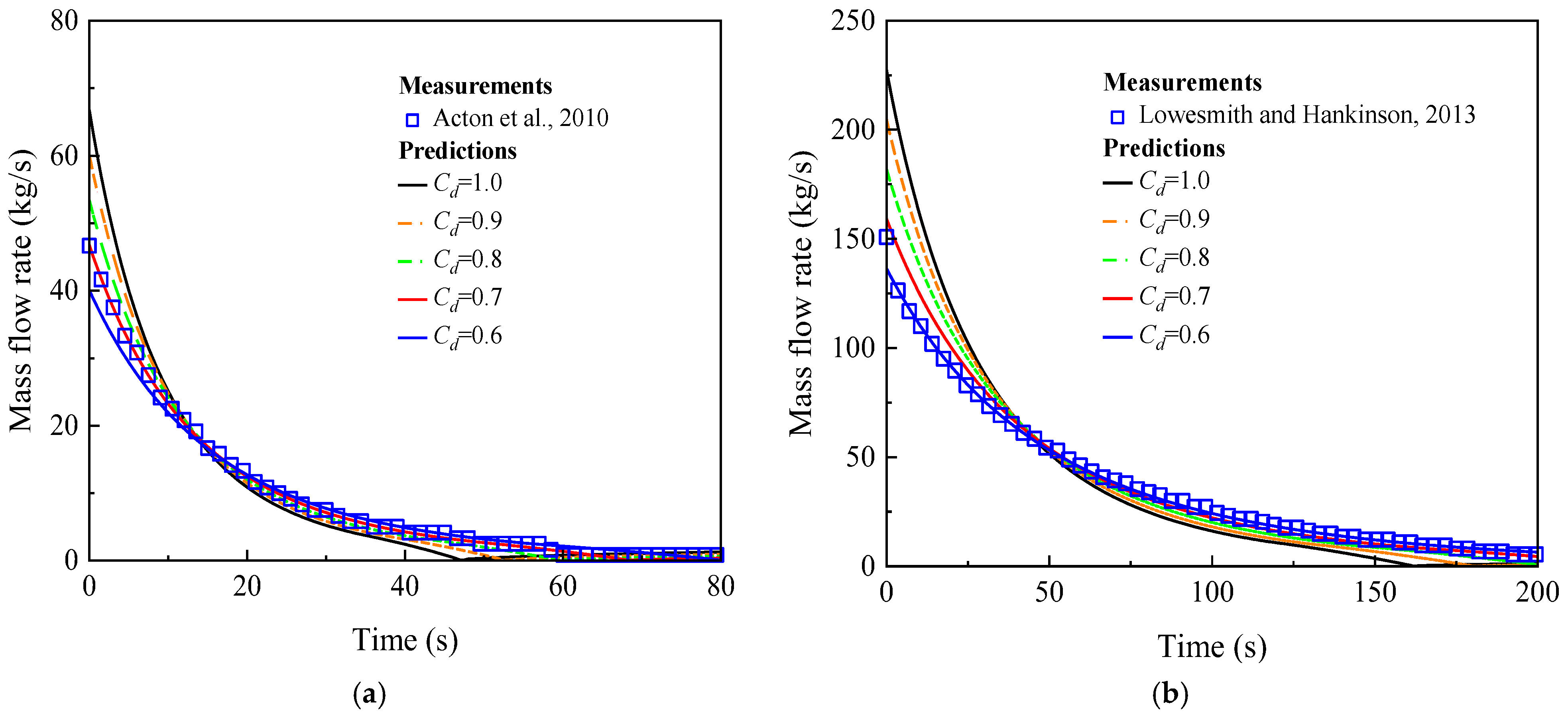
2.2. Verification of High-Pressure Gas Transient Leakage Model

To prove the rationality and correctness of the high-pressure gas transient leakage model [27], the mass flow rates in two high-pressure pipeline gas leakage jet fire experiments are calculated. In the process of the high-pressure gas leakage, the mass flow rates at the leakage outlet show a decreasing trend, as shown in Figure 2, which are, respectively, the mass flow rate obtained by Acton’s experiment and Lowesmith’s experiment. Note that the pure methane is used as an alternative fuel for theoretical calculations or numerical simulations in this work. In practice, the gas flow through the pipe will produce energy loss, so the discharge coefficient is considered to calculate the mass flow rate. As shown in Figure 2a, comparing the mass flow rate measured by Acton’s experiment [13] with the calculations, the results show that without considering the discharge coefficient ( C d = 1.0), the calculated mass flow rates of the two experiments are significantly higher than the measured results. According to the work of Cirrone et al. [42], the results via CFD simulation agree with the measured results when the discharge coefficient is equal to 0.7. By adjusting the discharge coefficient from 0.9 to 0.6, the calculated and measured results are compared. When the discharge coefficient is 0.7, the calculation results of the mass flow rate agree with the measurement obtained by Acton’s experiment (Figure 2a). The calculated mass flow rate for C d = 0.6 has a good agreement with the measurement obtained by Lowesmith’s jet fire experiment (Figure 2b). The results show that the discharge coefficient in the process of high-pressure gas leakage will cause a deviation to the mass flow rate, which will also affect the simulation results. Therefore, the discharge coefficient is taken into account in the numerical simulation.

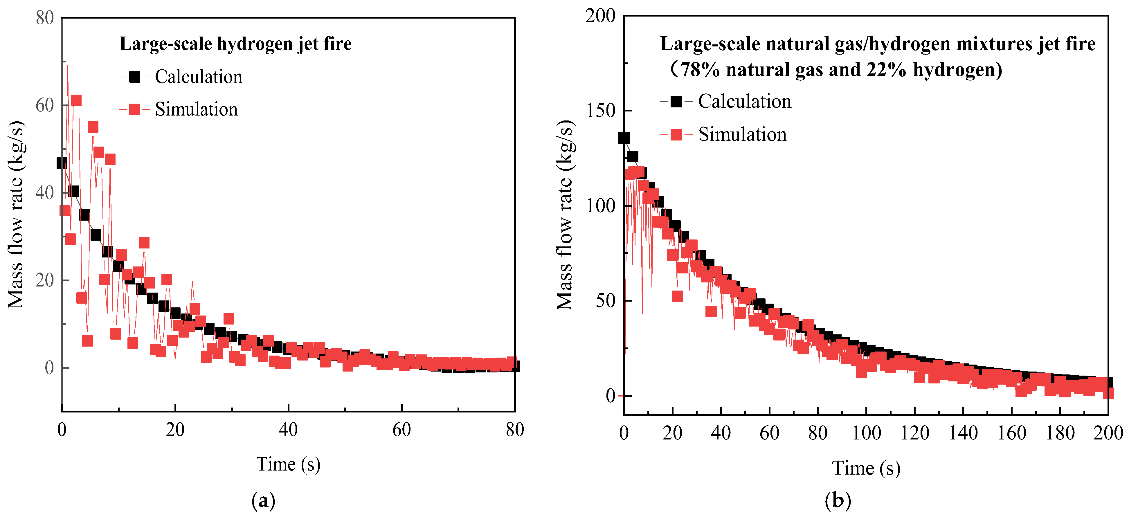
2.3. Verification of Equivalent Pipe Leakage Model

According to the two experimental cases, the ruptured pipe buried in the crater had two outlets, and the jet flowed from the two outlets after the pipeline ruptured. Under high-pressure conditions, the jets flowing from the outlets on both sides impinged in the middle of the pipe. The flow field temperature nephogram and streamline at 2 s after the high-pressure hydrogen leakage and 2 s after the high-pressure natural gas/hydrogen mixtures leakage are shown in Figure 3. Three velocity monitoring points are set 0.4 m away from the left leakage point, 0.4 m away from the right leakage point and at the point of the jet impact, respectively. By monitoring the instantaneous velocity of these three points, the flow velocity at the jet impact point is smaller than the jet flow velocity before the impact in both cases (Figure 4). The black spot in the temperature nephogram is located 2 m above the middle point of the pipe rupture section. The mass flow rate at the black point is monitored for comparison with the calculations applying the equivalent pipe leakage model (Figure 5). According to the jet impact and flow trajectory in the temperature nephogram (Figure 3), it is speculated that approximately half of the jet will flow downward after the impingement of the jet on both sides. Therefore, the mass flow rate at the black spot is consistent with the variation in the sum of the mass flow rates on both sides after the loss. As shown in Figure 5, the calculation results by the model tend to be consistent with the simulation results. This proves the reliability of the established equivalent pipe leakage model.

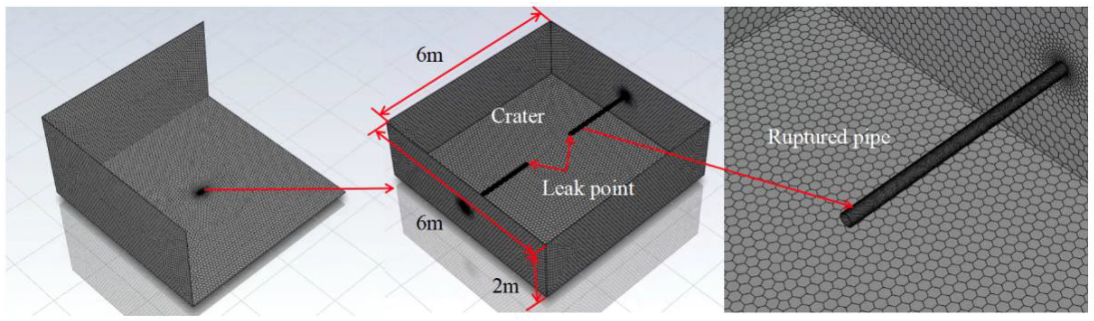
3. Numerical Modeling

3.1. Jet Fire Model

ANSYS Fluent 2020 R2 [47] is used for the CFD simulation. A 3D model of the crater, the ruptured pipe and the grid computing domain are built (Figure 6). The entire computational domain is 300 m long, 300 m wide and 152 m high. The computational mesh is divided using the Fluent Meshing, and the Mosaic (polyhedron–hexahedron core) mesh generation method is used to generate the three-dimensional mesh. It can complete the layered polygonal mesh near the wall, the pure polygonal mesh in the transition zone and the hexahedral mesh in the core area to fill the computational domain, which improves the overall quality level of the mesh and greatly reduces the total number of meshes and calculation time. Since the experimental case to be simulated is a large-scale experiment, the grid processing needs to comprehensively consider the accuracy of the simulation, the affordability of computer software and hardware and the simulation time. The dynamic process of gas in the ruptured pipe is complex, and the densest grid processing is needed. In addition, to save computing time, the area generated by the jet flame is divided into three sections, and the degree of mesh sizing is decreased from the bottom to the top. After grid processing, the optimal number of grids for the two experimental models is 2,955,007 and 2,400,934, respectively. To verify the independence of the grid and reduce the calculation time, three sets of grids are established for the two large-scale jet fire experiments. The number of grid cells is 2,116,299, 2,955,007 and 5,586,630 and 2,119,629, 2,400,934 and 5,589,168, respectively. As shown in Figure 7a,b, the results of the three grids selected in the two cases are similar. Considering the computing time, 2,955,007 grid cells and 2,400,934 grid cells are selected. The method of the spatial discrete second-order upwind format is adopted. The time step is set to 0.5 s, and the independence of the time step is verified by comparing the flame temperature at different distances from the flame center line when the time step is 0.1 s, 0.5 s and 1 s. The difference between the time step of 0.5 s and 0.1 s is small (Figure 7c,d). In order to shorten the calculation time, the time step is selected to be 0.5 s. The boundary condition of the leak point is set as the mass flow rate inlet, and the boundary condition of the ground, ruptured pipe and crater are set as the walls. The wind direction is achieved by setting one side of the computational domain as the velocity inlet (e.g., the westerly is realized by setting the western boundary condition as the velocity inlet), and the wind speed can be adjusted. The rest are set as the pressure outlet.
In the large-scale hydrogen jet fire experiment, four radiant heat flow meters are placed 40 m, 50 m, 60 m and 80 m south, respectively (Figure 8). In the large-scale natural gas blended with hydrogen jet fire experiment, three radiant heat flow meters are placed 40 m, 76 m and 144 m southwest, respectively (Figure 8).

3.2. Turbulence Model

When the fluid velocity is large, the adjacent layers are mixed with each other, resulting in irregular turbulent motion. Turbulence models include a two-equation model ( k ε , k ω ) and combined models such as shear-stress transport (SST) and baseline (BSL) models [48]. In the simulation, the RNG k ε model is selected as the turbulence model. Like the realizable k ε model, the RNG k ε model is also derived from the standard k ε model [49]. Due to its simplified Reynolds stress model assumption, the RNG k ε model lacks a suitable prediction of the turbulence length/time scale [50,51]. The RNG   k ε model uses a formula for considering a flow viscosity with a low Reynolds number [52,53,54]. Compared with the standard k ε model, the analytical derivative of the model can provide results using different constants [55]. The transport equations of the RNG k ε model are as follows:
t ρ k + x i ρ k u i = x j α k μ e f f k x j + G k + G b ρ ε Y M + S k
t ρ ε + x i ρ ε u i = x j α ε μ e f f ε x j + C 1 ε ε k G k + C 3 ε G b ρ C 2 ε ε 2 k R ε + S ε
where α k and α ε are the inverse effective Prandtl numbers for k and ε , and G k and G b represent the turbulent kinetic energy generated by the mean velocity gradients and buoyancy, respectively [56]. Y M represents the contribution of the compressible turbulent pulsating expansion to the overall dissipation rate, and S k and S ε are user-defined source terms [47,56]. C 1 ε , C 2 ε and C 3 ε are constants.

3.3. Combustion Model

Different from the EDC combustion model, which is not fit for large-scale experiments, the non-premixed combustion model can obtain a higher computational efficiency and is more fit for large-scale experiments [54]. To find a more suitable combustion model, the experimental data of Schefer et al. [57] are introduced, and the simulated results of the center line temperature distributions are compared with the experimental data. According to Figure 9, the non-premixed combustion model is more consistent with the experimental results, and the non-premixed combustion model has two sub-models: the chemical equilibrium model and the steady diffusion flamelet model. The calculation times of the two non-premixed combustion models are 83 min and 101 min, respectively. Therefore, the non-premixed chemical equilibrium combustion model is chosen due to its lower computational demand. Both the non-premixed chemical equilibrium combustion model and the non-premixed steady diffusion flamelet model can simulate the reaction of turbulent diffusion flames. The non-premixed chemical equilibrium combustion model can balance the chemical reaction quickly and calculate the intermediate components. Moreover, it can achieve chemical equilibrium better than the steady diffusion flame surface model. The local chemical equilibrium of the steady diffusion flame surface model has an unbalanced effect, leading to untrue results. Under the same simulation effect, the chemical equilibrium model is more stable and efficient. Non-premixed combustion can solve the equations of multiple species, which is a very suitable combustion model with mixed gas as fuel. In the non-premixed model, the mixing fraction affects the instantaneous thermochemical state of the fluid. The mixture fraction f can be expressed by the atomic mass fraction, where Z c is the mass fraction of component c, Z c , o x is the mass fraction of the oxidant inlet and Z c , f u e l is the mass fraction of the fuel inlet as shown below [47,58,59]:
f = Z c Z c , o x Z c , f u e l Z c , o x
The assumption of moderate diffusivity in turbulent motion can hold under this assumption of equal diffusivity, and the equation for the mixture fraction is a single conservation equation as shown below [47]:
t ρ m f ¯ + · ρ m v f ¯ = · λ C p + μ t σ t f ¯ + S m + S u s e r
Among them, ρ m is the mixture density, v is the mixture velocity, λ is the thermal conductivity of the mixture, C p is the specific heat capacity of the mixture, μ t is the turbulent viscosity, σ t is the Prandtl number, S m is the source term and S u s e r is any user-defined source term [47,60].
In addition to solving for the Favre mean mixture fraction, a conservation equation for the mixture fraction variance ( f 2 ¯ ) is solved using ANSYS Fluent [47]:
t ρ m f 2 ¯ + · ρ m v f 2 ¯ = · λ C p + μ t σ t f 2 ¯ + C g μ t · f ¯ 2 C d ρ m ε k f 2 ¯ + S u s e r
The mixture fraction variance is used in the closure model that describes turbulence–chemistry interactions, where f = f f ¯ and the default values for the constants σ t , C g and C d are 0.85, 2.86 and 2.0, respectively.

3.4. Radiation Model

The P-1 radiation model is chosen as the radiation model. The P-1 model is a simplification of the RTE model [61]. The P-1 model has low CPU requirements [62]. It belongs to the simplest type of P-N model, which can handle the radiation problem of complex geometries and consumes less resources [50]. The radiation flux q r in the P-1 radiation model can be expressed as follows:
q r = 1 3 a + σ s C σ s G
To simplify the radiation flux formula, the parameter Γ is introduced:
Γ = 1 3 a + σ s C σ s
Thus, Equation (28) is added into Equation (27):
q r = Γ G
The transport equation for the incident radiation G can be expressed as follows [63]:
· Γ G a G + 4 a n 2 σ T 4 = S G
Combine Equation (29) and Equation (30) to obtain the following:
· q r = a G 4 a n 2 σ T 4
In the above equations, a is the absorption coefficient, σ s is the scattering coefficient, C is the linear-anisotropic phase function coefficient, G is the incident radiation, n is the refractive index of the medium, σ is the Stefan–Boltzmann constant and S G is a user-defined radiation source [47].

4. Results and Discussion
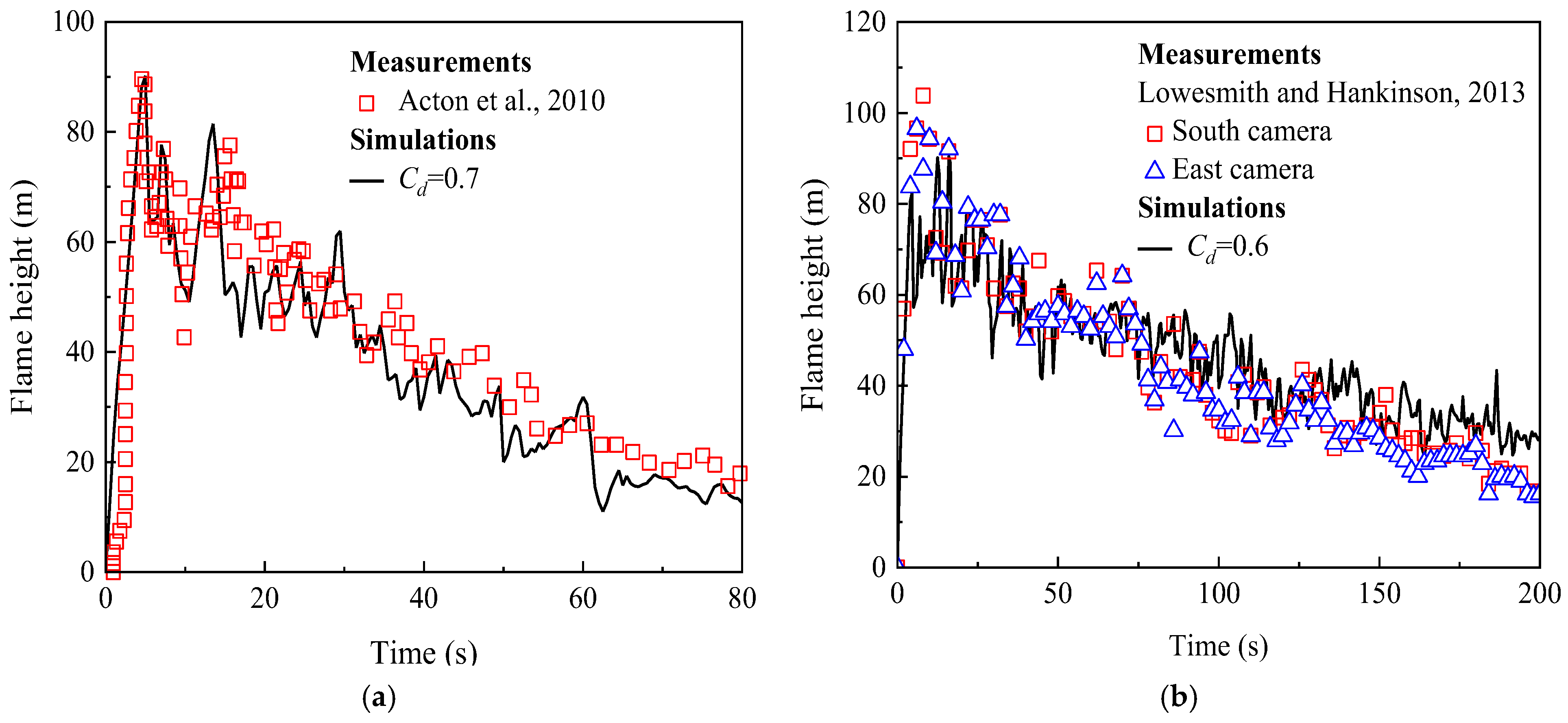
4.1. Flame Height

The experimental data are obtained from the high-pressure hydrogen pipeline leak jet fire experiment [13] and the high-pressure natural gas blended with hydrogen pipeline leak jet fire experiment, respectively [16]. The initial pressure in the hydrogen storage pipe is 6.1 MPa. The wind speed in open space is 4–8 m/s. The wind direction is variable. The ambient temperature is 298 K. Lowesmith and Hankinson set up a similar test platform. In Case 2, the initial pressure in the pipe is 7.16 MPa. The wind direction is northwest. The wind speed is 1–2 m/s. The ambient temperature is 277 K. The two experiments are both conducted at atmospheric pressure (0.1 MPa). Table 1 shows the experimental parameters of these two cases.
As shown in Figure 10a,b, the simulation results of flame height versus the leakage time in Cases 1 (hydrogen) and 2 (natural gas/hydrogen mixtures) are compared with the experimental data. It is worth noting that in Case 1, the measured data of the flame height are not consistent with the simulated results in the first 2 s, and the measurement data are always 0 in the first 0.5 s, while the simulated flame height began to increase from 0. The reason is that in the large-scale hydrogen jet fire experiment, the jet fire had not yet formed at the moment of the hydrogen leakage. Meanwhile, in the simulation, the simulated hydrogen jet fire is ignited at the moment of the leakage to form a jet fire. Figure 10a shows that the flame height through the CFD simulation is consistent with the measured data after 2 s. The monitoring of the flame height in the simulation is achieved by monitoring the grid height of the 1500 K isotherm [42].
The flame heights are observed in the experiment of Lowesmith and Hankinson [16] from both the south and east. The trend of the flame height throughout the simulation is consistent with that of the measuring result monitored from the east and south, as shown in Figure 10b. In the simulation, the influence of resistance loss is considered, and the mass flow rate for C d = 0.6 is selected as the boundary condition. In the simulation process of the above two experiments, the notional nozzle model is applied. The maximum value of the simulated flame height in Case 2 is lower than the measured data. It is speculated that a huge fireball is formed in the first stage of the high-pressure gas leakage. This process is not incorporated into the current simulation.

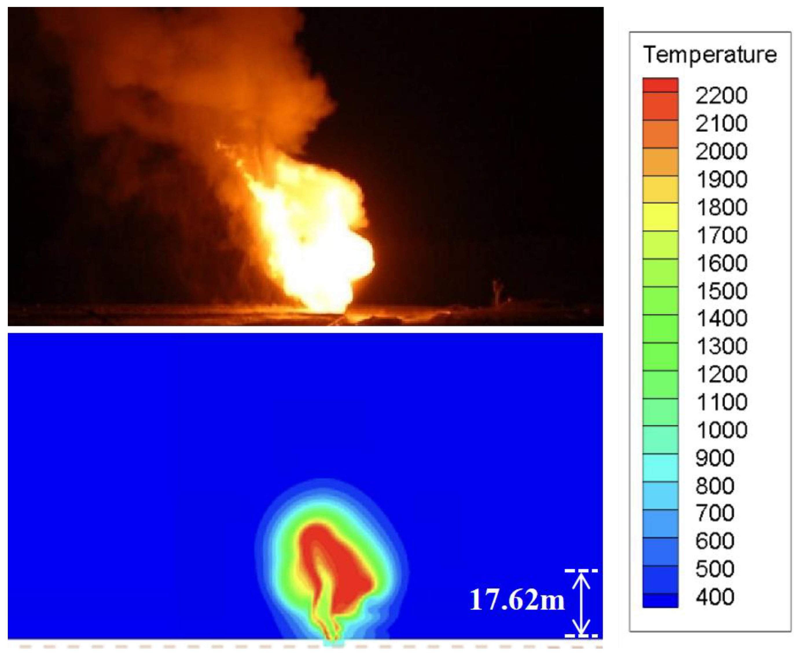
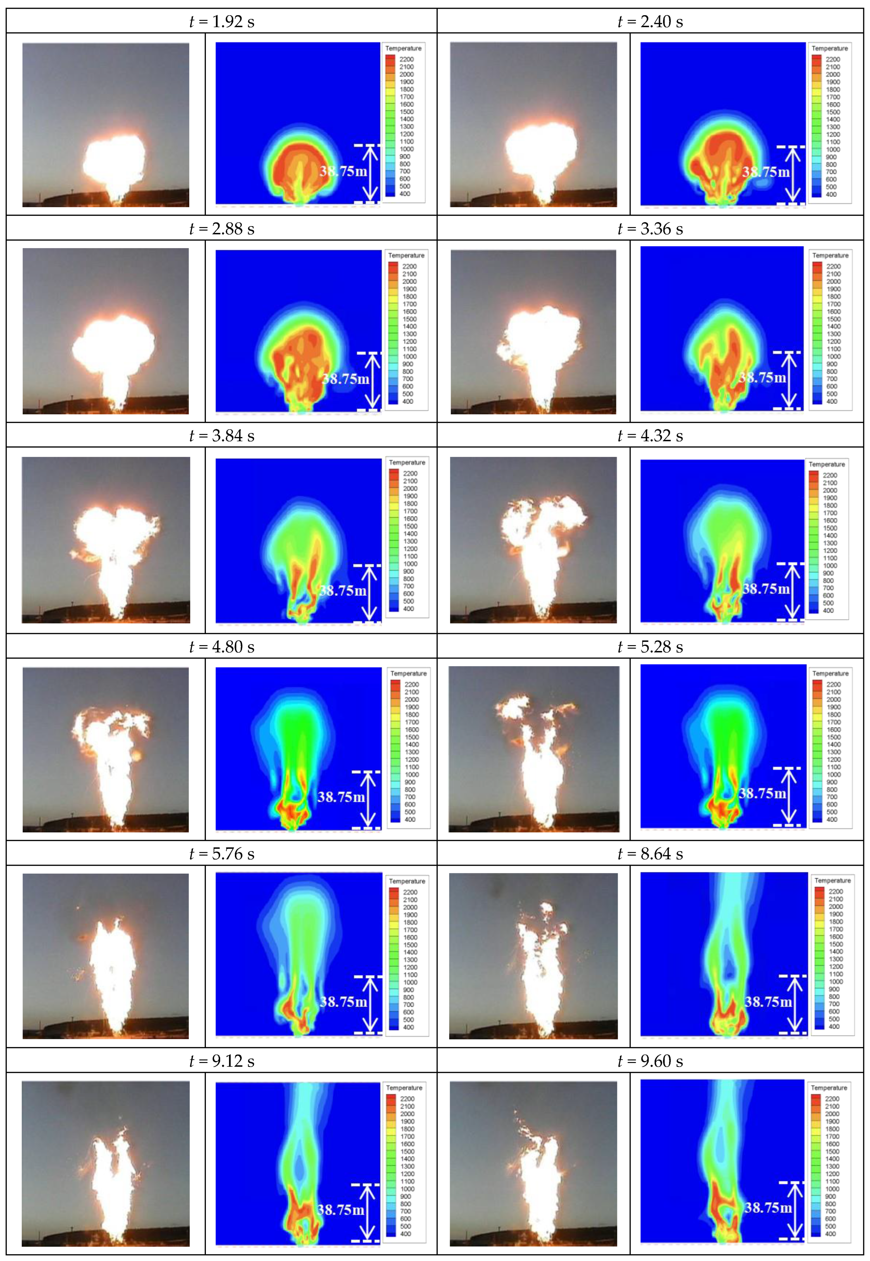
4.2. Flame Appearance

When comparing the simulated flame’s appearance with the measured results by Acton et al. [13], for which the flame temperature is 400–2200 K, the simulated results are consistent with the experimental results. Figure 11 shows an image of the flame taken shortly after the ignition of the pipeline leak. In the experiment, a fireball with a short duration is formed at the moment of the hydrogen pipeline leakage. After the gas is ignited, a transient flame is formed. With the attenuation of the gas flow, the flame height is continuously reduced. Comparing the flame temperature contours at different time points in the simulation shortly after the leakage, the flame’s appearance throughout the simulation at 1.5 s after the leakage is consistent with the flame’s appearance in the experiment (Figure 11). The simulated flame and the experimental flame are tilted by the influence of ambient wind.
Lowesmith’s experimental images are also consistent with the simulation results. The measured results show the flame’s appearance at some moments in the first 10 s. By selecting the flame temperature cloud diagram at the corresponding moment in the simulation, the flame’s appearance through the simulation in these 10 s is basically the same as the flame’s appearance from the experiment (Figure 12). Based on the previous work of Cirrone et al. [42] and Mahmud et al. [64], a temperature contour of 1500 K is used to define the flame height. By observing the experimental flame image and the simulated flame temperature cloud diagram, within 4 s after the leakage, the leaked gas is ignited, rapidly expands to form a fireball and continues to expand and rise. Five to eight seconds after the leakage, the height of the fireball reaches the maximum of about 100 m, and then a jet flame is formed with a gradual decrease in height with the leakage time. As the gas pressure in the pipeline decreases, the mass flow rate continues to decrease, and the jet flame height gradually decreases. When the fireball is extinguished, a small amount of soot is produced, and the flame is yellow as a whole. By comparing the flame height and flame appearance between the simulation and the experiment, the accuracy of the simulation of the flame size is proven.

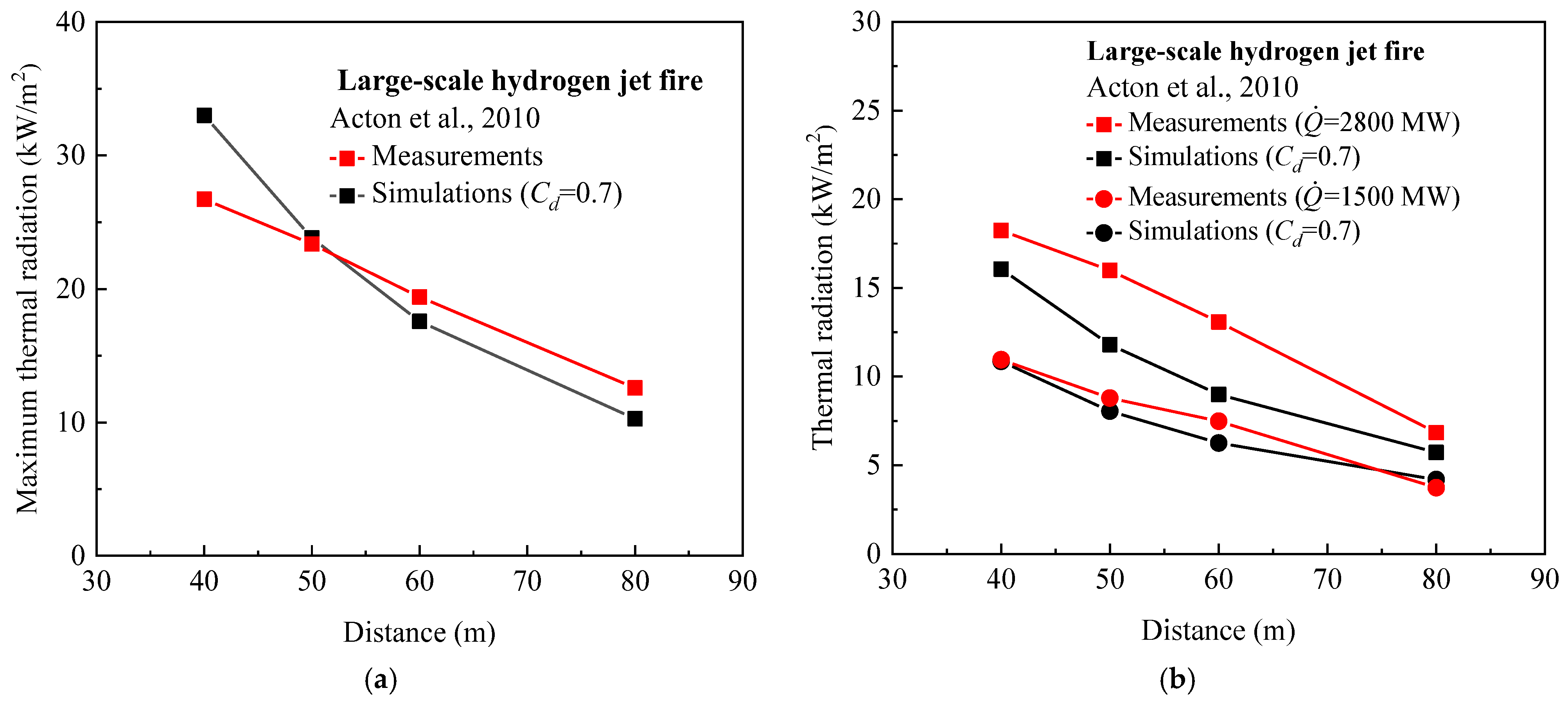
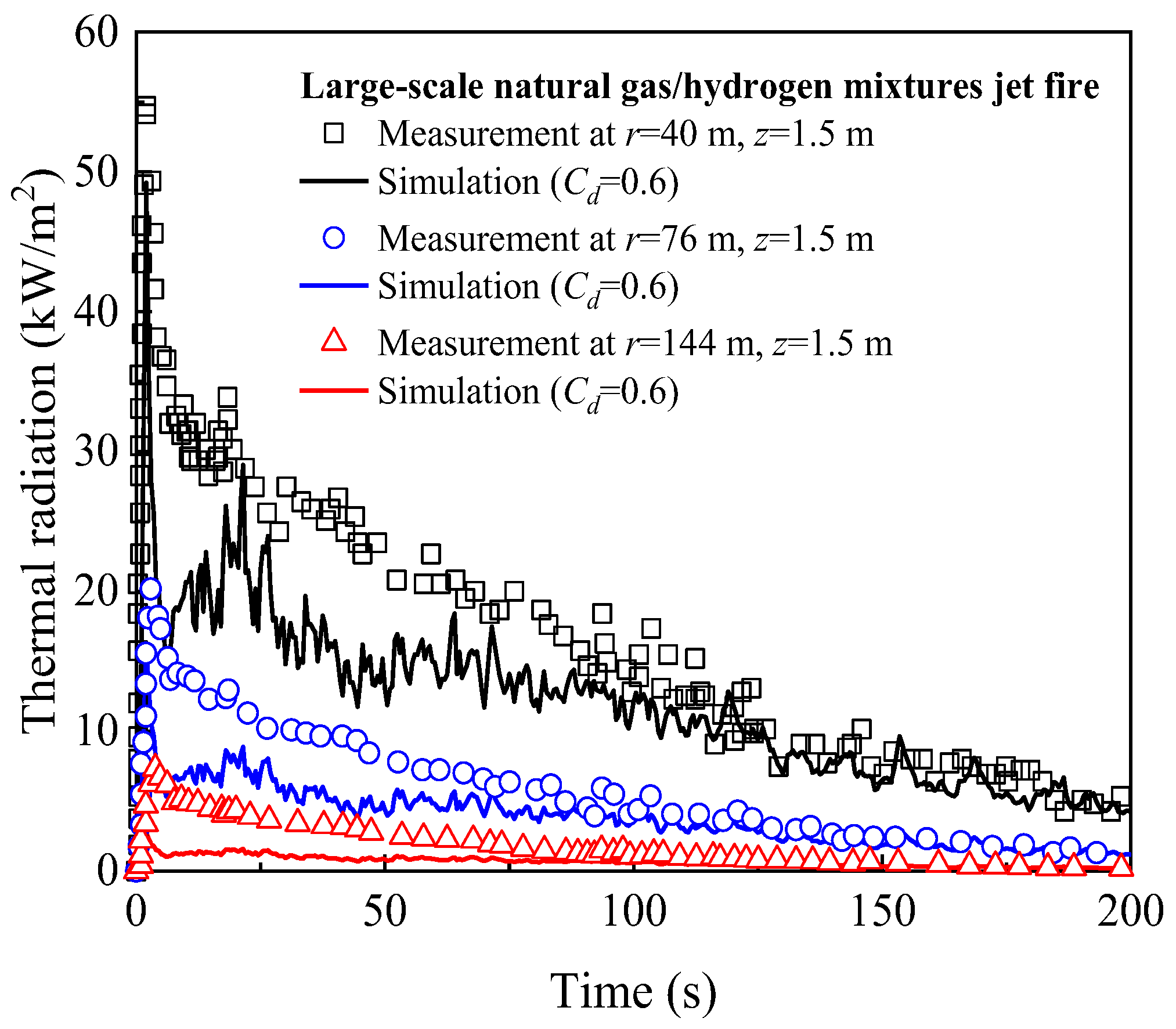
4.3. Thermal Radiation

Figure 13 shows the comparison between the experimental data and simulated results of the thermal radiation variation with the measured distance of the high-pressure hydrogen jet flame. As shown in Figure 13a, the simulated results of the maximum thermal radiation within 80 s agree with the measured data. The simulated results of the maximum thermal radiation at 40 m and 50 m are higher than the measured data, but the simulated results of the maximum thermal radiation at 60 m and 80 m from the central axis of the flame are slightly lower than the measured data. Figure 13b shows the relationship of the thermal radiation throughout the simulation and the measurement at the flame heat release rates of 2800 MW and 1500 MW, respectively. For the heat release rate of 2800 MW (at t = 11.5 s), the simulations of the flame thermal radiations at four different measured distances (i.e., 40 m, 50 m, 60 m and 80 m, respectively) are slightly lower than the measured data as a whole, and the simulated flame thermal radiations at 40 m and 80 m are much closer to the measurements. When the heat release rate is 1500 MW (at t = 20.5 s), the simulated results of the flame thermal radiations at four different measured distances are quite consistent with the measured data. From the comparison between the measured and simulated results of the maximum thermal radiation and the thermal radiation at different heat release rates, it can be concluded that the overall variation trend of the simulations of the flame thermal radiation is consistent with the experimental measurement. This further proves the accuracy of the proposed method for predicting the thermal radiation of jet fires resulting from hydrogen and hydrogen-blended natural gas pipeline leaks.
Figure 14 shows a comparison of the variation in the thermal radiation with the leakage time between the simulation and the experiment conducted by Lowesmith and Hankinson [16]. It can be seen from Figure 14 that the simulated results of the flame thermal radiation are generally lower than the measured data in the previous stage. In particular, the simulated maximum thermal radiation of the jet fire at 144 m is lower than the experimental data. According to the scene photos of Lowesmith’s experiment, a spherical flame is produced in the previous stage, which radiated strong heat fluxes. But in the simulation, the gas leakage immediately ignites to form a stable jet fire, and this dynamic process cannot be accurately monitored. Thus, the simulated results of the flame thermal radiation in the previous stage are generally lower than the measured data. However, after 100 s, the simulated flame thermal radiations are consistent with the measured data. In general, the overall variation trend of the simulated thermal radiation from the jet fires is consistent with the experimental measurements.

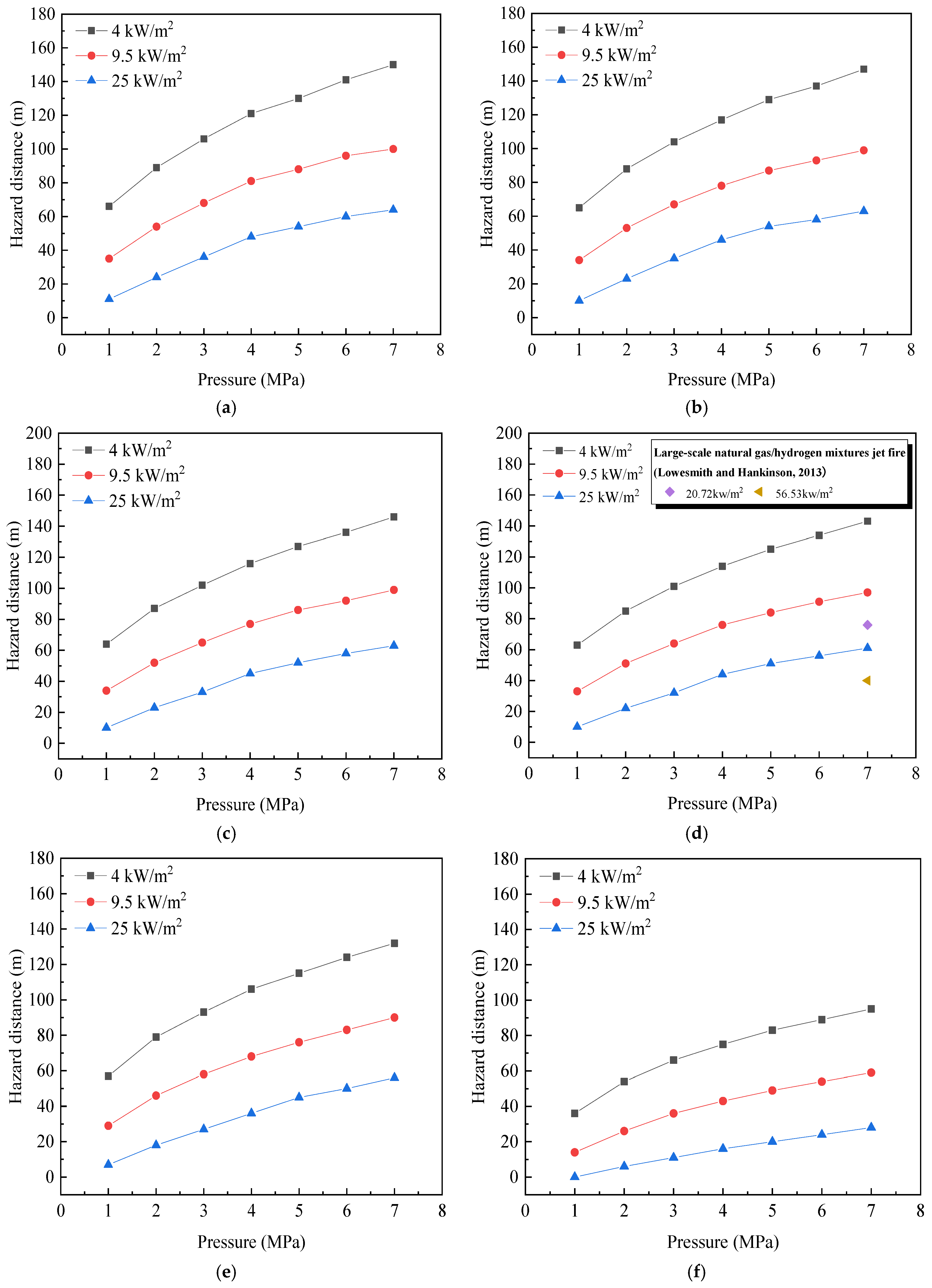
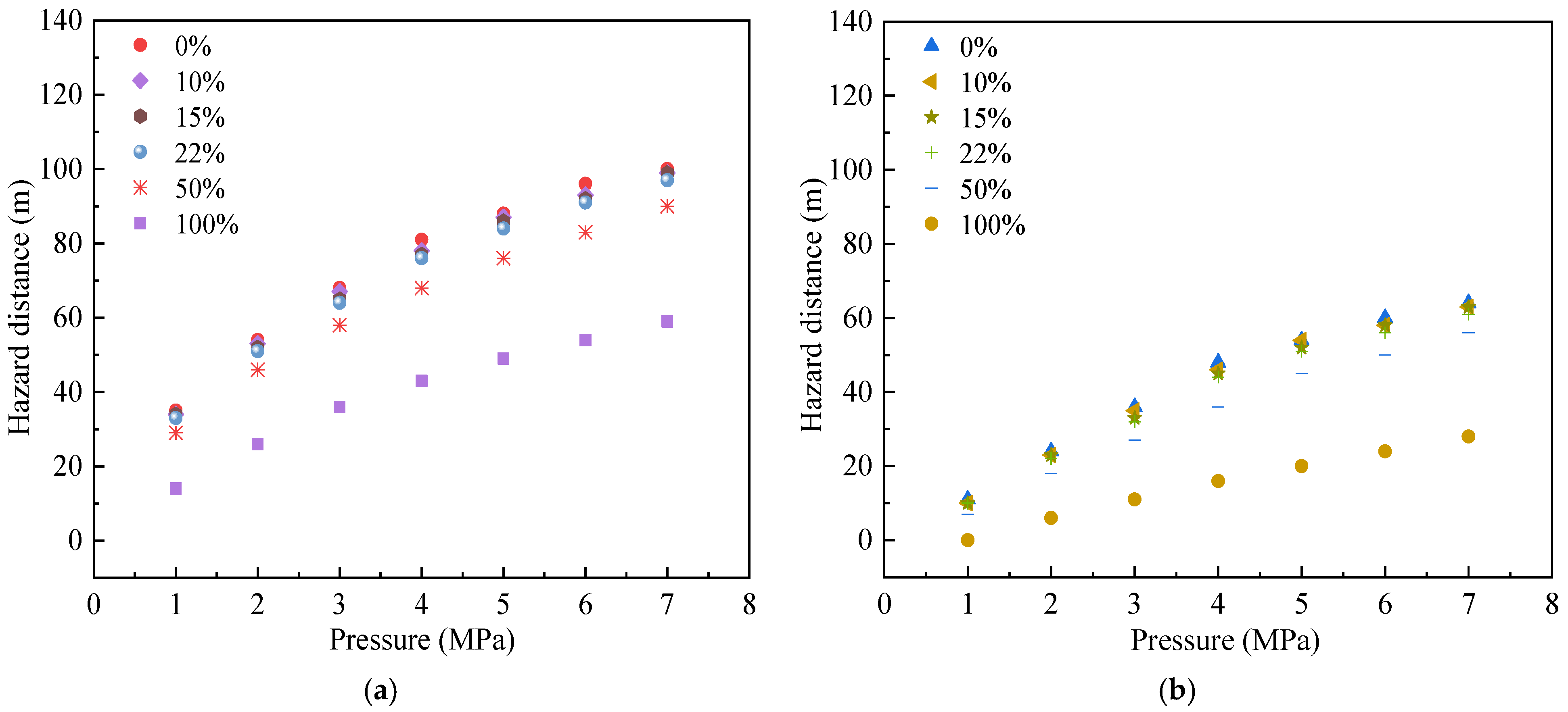
4.4. Hazard Distance of Thermal Radiation

The thermal radiation of jet flames can cause serious damage to the human body, so it is crucial to know the distances at which thermal radiation causes harm. According to the literature [65], the different hazard degrees of thermal radiation flux have different hazard distances. Table 2 presents the hazard criteria for evaluating thermal radiation and hazard distances.
According to the simulation results, the hazard distances caused by high-pressure hydrogen jet fire (Case 1) and high-pressure natural gas/hydrogen mixture jet fire (Case 2) under different heat radiation fluxes are obtained, as shown in Figure 15. According to the simulation results, the high-pressure hydrogen jet fire will cause 100% lethality in 1 min within 46 m from the center line of the flame, second-degree burns within 76 m and first-degree burns within 107 m. The high-pressure natural gas/hydrogen mixture jet fire will cause 100% lethality in 1 min within 61 m from the center line of the flame, second-degree burns within 97 m and first-degree burns within 143 m.
To further study the influence of different pipe pressures and hydrogen blending ratios on the hazard distances of flame thermal radiation, seven different pipe pressures and six different hydrogen blending ratios are considered, and the corresponding hazard distances are analyzed (Figure 16). The pipe diameter and environmental parameters are the same as those in Case 2. The pressure in the pipe is increased from 1 MPa to 7 MPa, and the hydrogen blending ratio is set to 0%, 10%, 15%, 22%, 50% and 100%, respectively. As show in Figure 16a–e, when the hydrogen blending ratio is constant, the hazard distance increases with the increase in pressure. When the pressure is constant, the hazard distance decreases with the increase in the hydrogen blending ratio. In Figure 16d, the experimental data of the thermal radiation hazard distance of the natural gas/hydrogen mixture jet fire with a hydrogen blending ratio of 22% conducted by Lowesmith [16] are added. By comparing the 40 m hazard distance corresponding to a thermal radiation of 56.5 kW/m2 and the 76 m hazard distance corresponding to a thermal radiation of 20.7 kW/m2 with the simulated hazard distance, the overall variation trend of the hazard distance with the thermal radiation is consistent. The results show that the proposed simulation framework is reliable in judging the hazard distance of the thermal radiation. When the hydrogen blending ratio increases from 0% to 22%, the hazard distance under the corresponding thermal radiations of 4 kW/m2 and 9.5 kW/m2 decreases by 5% and 2%, respectively (Figure 17). When the hydrogen blending ratio increases from 0% to 50%, the hazard distance under the corresponding thermal radiations of 4 kW/m2 and 9.5 kW/m2 decreases by 14% and 11%, respectively (Figure 17). It proves that the decrease in the thermal radiation hazard distance is less affected by the hydrogen blending ratio when the hydrogen blending ratio is lower than 22%. The flame thermal radiation hazard distance is affected by the mass flow rate of leaked gas. After natural gas is mixed with hydrogen, the density of mixed gas is smaller than that of natural gas, and its density decreases with the increase in the hydrogen blending ratio. Thus, under the same pipe diameter and pressure, the mass flow rate of the natural gas/hydrogen mixtures is lower than that of the natural gas and decreases with the increase in the hydrogen blending ratio. Meanwhile, the gas diffusion combustion coefficient of hydrogen is lower than that of natural gas, resulting in a decrease in the thermal radiation intensity of the mixed gas. Therefore, the increase in the hydrogen blending ratio can lead to a reduction in the flame thermal radiation hazard distance.

5. Conclusions

A 3D model of a pipeline leakage jet fire accident involving a gas mixture is established with ANSYS Fluent 2020 R2. The problem of the prediction of gas mass flow rates in the actual pipeline leakage situation due to the jet impingement is solved by establishing an equivalent pipe leakage model.
The non-premixed chemical equilibrium combustion model is validated to be a more suitable combustion model by comparing the simulated results of the flame center line temperature distributions with the experimental results. A CFD simulation framework is obtained by using the RNG k ε turbulence model, the non-premixed chemical equilibrium combustion model and the P-1 thermal radiation model for large-scale high-pressure gas leakage jet fires. The simulated results of the flame height, flame appearance and flame thermal radiation agree with the experimental results to verify the reliability of the proposed model and the CFD simulation framework.
When the hydrogen blending ratio is the same, the thermal radiation hazard distance increases with the pressure (from 1 MPa to 7 MPa). When the pressure is the same, the thermal radiation hazard distance decreases with the hydrogen blending ratio, increasing from 0% to 100%. When the hydrogen blending ratio is lower than 22%, the decrease in the thermal radiation hazard distance is less affected.
The simulation and accurate estimation of high-pressure gas leakages and the resulting jet fire radiation are very significant in process industries. It is helpful for the design of pipelines transporting pure hydrogen or hydrogen blended with natural gas and the determination of safe distances from these pipelines. This work supports the reliability of the CFD simulation of pipeline leakage and gas combustion, leading to more accurate predictions of large-scale jet fires induced by the leakage of high-pressure pure hydrogen and hydrogen-blended natural gas pipelines. In the future, other influential factors, such as the pipeline diameter and wind speed, etc., should be explored.

Author Contributions

Conceptualization, Z.W. and J.J.; Methodology, Z.W.; Validation, G.W.; Data curation, W.L.; Writing—original draft, M.L.; Writing—review & editing, Z.W.; Supervision, Z.W., L.N. and Y.P. All authors have read and agreed to the published version of the manuscript.

Funding

This work was financially supported by the Jiangsu Provincial Key R&D Programme-Social Development (No. BE2023809), Natural Science Foundation of Jiangsu Province (No. BK20230318), China Postdoctoral Science Foundation (No. 2022M711603), Jiangsu Funding Program for Excellent Postdoctoral Talent (No. 2022ZB388), and Natural Science Foundation of the Jiangsu Higher Education Institutions of China (No. 22KJB620005). ZH acknowledges support from the Nanjing Science and Technology Innovation Key Project for the Returned Overseas Scholars (Class A).

Institutional Review Board Statement

Not applicable.

Informed Consent Statement

Not applicable.

Data Availability Statement

The raw data supporting the conclusions of this article will be made available by the authors on request.

Conflicts of Interest

The authors declare no conflicts of interest.

Nomenclature

ALeakage area (m2)
bCorrection coefficient of gas specific volume (m3/kg)
CdDischarge coefficient
dDiameter (m)
mGas mass (kg)
m ˙ Gas mass flow rate (kg/s)
PGas absolute pressure (Pa)
R g Gas constant (J/(kg·K))
TGas thermodynamic temperature (K)
uGas flow velocity (m/s)
vGas specific volume (m3/kg)
v c r Critical pressure ratio
t Time (s)
u i Velocity components in x-direction (m/s)
x i Physical coordinate in x-direction
x j Physical coordinate in y-direction
k Turbulence kinetic energy (m2/s2)
Y M Contribution of the fluctuating dilatation in compressible turbulence to the overall dissipation rate
G k Turbulent kinetic energy generation term due to the mean velocity gradient
G b Turbulence kinetic energy generation term due to buoyancy
S Source term
C 1 ε Constant = 1.42
C 2 ε Constant = 1.68
C 3 ε Constant
Z Mass fraction (%)
f Mixture fraction (%)
v Mixture velocity (m/s)
λ Thermal conductivity (W/(m·K))
C p Specific heat capacity (J/(kg·K))
q r Radiation flux (kW/m2)
Γ Parameter in Equation (28)
G Incident radiation (kW/m2)
C Linear-anisotropic phase function coefficient
n Refractive index of the medium (cm−1)
a Absorption coefficient (cm−1)
r Distance from the flame center line (m)
z Height from the ground (m)
Q ˙ Heat release rate (MW)
Greek symbols
ρ Gas density (kg/m3)
γ Specific heat ratio
ε Turbulence eddy dissipation (m2/s3)
σ s Scattering coefficient (cm−1)
σ Stefan–Boltzmann constant = 5.67 × 10⁻⁸ (W/(m2·K4))
μ t Turbulent viscosity (kg/(m·s))
σ t Prandtl number
α Inverse effective Prandtl number
μ dynamic viscosity (Pa·s)
Subscripts
a Ambient gas condition
iIteration
0Initial
1Gas state inside the pipe
2Gas state at the real leakage outlet
3Gas state at the notional nozzle
c Component
o x Oxidant inlet
m Mixture
u s e r User-defined
f u e l Fuel inlet

References

  1. Al-Breiki, M.; Bicer, Y. Comparative life cycle assessment of sustainable energy carriers including production, storage, overseas transport and utilization. J. Clean. Prod. 2021, 279, 123481. [Google Scholar] [CrossRef]
  2. Olabi, A.G.; Abdelkareem, M.A. Renewable energy and climate change. Renew. Sust. Energ. Rev. 2022, 158, 112111. [Google Scholar] [CrossRef]
  3. Li, Y.; Kuang, Z.; Fan, Z.; Shuai, J. Evaluation of the safe separation distances of hydrogen-blended natural gas pipelines in a jet fire scenario. Int. J. Hydrogen Energy 2023, 48, 18804–18815. [Google Scholar] [CrossRef]
  4. Olabi, A.G.; Abdelkareem, M.A.; Mahmoud, M.S.; Elsaid, K.; Obaideen, K.; Rezk, H.; Wilberforce, T.; Eisa, T.; Chae, K.-J.; Sayed, E.T. Green hydrogen: Pathways, roadmap, and role in achieving sustainable development goals. Process Saf. Environ. Protect. 2023, 177, 664–687. [Google Scholar] [CrossRef]
  5. Renssen, S.V. The hydrogen solution? Nat. Clim. Chang. 2020, 10, 799–801. [Google Scholar] [CrossRef]
  6. Global Hydrogen Review 2022; IEA: Paris, France, 2022.
  7. Ma, N.; Zhao, W.; Wang, W.; Li, X.; Zhou, H. Large scale of green hydrogen storage: Opportunities and challenges. Int. J. Hydrogen Energy 2024, 50, 379–396. [Google Scholar] [CrossRef]
  8. Su, Y.; Li, J.; Yu, B.; Zhao, Y. Numerical investigation on the leakage and diffusion characteristics of hydrogen-blended natural gas in a domestic kitchen. Renew. Energ. 2022, 189, 899–916. [Google Scholar] [CrossRef]
  9. Chen, X.; Zhang, C.; Li, Y. Research and development of hydrogen energy safety. Emerg. Manag. Sci. Technol. 2022, 2, 3. [Google Scholar] [CrossRef]
  10. Wang, Z.; Zhou, K.; Zhang, L.; Nie, X.; Wu, Y.; Jiang, J.; Dederichsc, A.S.; He, L. Flame extension area and temperature profile of horizontal jet fire impinging on a vertical plate. Process Saf. Environ. Protect. 2021, 147, 547–558. [Google Scholar] [CrossRef]
  11. Wang, C.; Zhang, L.; Tao, G. Quantifying the influence of corrosion defects on the failure prediction of natural gas pipelines using generalized extreme value distribution (GEVD) model and Copula function with a case study. Emerg. Manag. Sci. Technol. 2024, 4, e003. [Google Scholar] [CrossRef]
  12. Schefer, R.W.; Houf, W.G.; Williams, T.C.; Bourne, B.; Colton, J. Characterization of high-pressure, underexpanded hydrogen-jet flames. Int. J. Hydrogen Energy 2007, 32, 2081–2093. [Google Scholar] [CrossRef]
  13. Acton, M.R.; Allason, D.; Creitz, L.W.; Lowesmith, B.J. Large scale experiments to study hydrogen pipeline fires. In Proceedings of the 2010 8th International Pipeline Conference, Calgary, AB, Canada, 27 September–1 October 2010; pp. 593–602. [Google Scholar]
  14. Proust, C.; Jamois, D.; Studer, E. High pressure hydrogen fires. Int. J. Hydrogen Energy 2011, 36, 2367–2373. [Google Scholar] [CrossRef]
  15. Lowesmith, B.J.; Hankinson, G. Large scale high pressure jet fires involving natural gas and natural gas/hydrogen mixtures. Process Saf. Environ. Protect. 2012, 90, 108–120. [Google Scholar] [CrossRef]
  16. Lowesmith, B.J.; Hankinson, G. Large scale experiments to study fires following the rupture of high pressure pipelines conveying natural gas and natural gas/hydrogen mixtures. Process Saf. Environ. Protect. 2013, 91, 101–111. [Google Scholar] [CrossRef]
  17. Wu, L.; Kobayashi, N.; Li, Z.; Huang, H.; Li, J. Emission and heat transfer characteristics of methane–hydrogen hybrid fuel laminar diffusion flame. Int. J. Hydrogen Energy 2015, 40, 9579–9589. [Google Scholar] [CrossRef]
  18. Hooker, P.; Hall, J.; Hoyes, J.R.; Newton, A.; Willoughby, D. Hydrogen jet fires in a passively ventilated enclosure. Int. J. Hydrogen Energy 2017, 42, 7577–7588. [Google Scholar] [CrossRef]
  19. Xiao, J.; Kuznetsov, M.; Travis, J.R. Experimental and numerical investigations of hydrogen jet fire in a vented compartment. Int. J. Hydrogen Energy 2018, 43, 10167–10184. [Google Scholar] [CrossRef]
  20. Tang, Z.; Wang, Z.; Zhao, K. Flame extension length of inclined hydrogen jet fire impinging on a water curtain. J. Loss Prev. Process Ind. 2023, 83, 105059. [Google Scholar] [CrossRef]
  21. Zhao, C.; Li, X.; Wang, X.; Li, M.; Xiao, H. An experimental study of the characteristics of blended hydrogen-methane non-premixed jet flames. Process Saf. Environ. Protect. 2023, 174, 838–847. [Google Scholar] [CrossRef]
  22. Yu, X.; Wang, C.J.; He, Q.Z. Numerical study of hydrogen dispersion in a fuel cell vehicle under the effect of ambient wind. Int. J. Hydrogen Energy 2019, 44, 22671–22680. [Google Scholar] [CrossRef]
  23. Markert, F.; Melideo, D.; Baraldi, D. Numerical analysis of accidental hydrogen releases from high pressure storage at low temperatures. Int. J. Hydrogen Energy 2014, 39, 7356–7364. [Google Scholar] [CrossRef]
  24. Cleaver, R.P.; Halford, A.R. A model for the initial stages following the rupture of a natural gas transmission pipeline. Process Saf. Environ. Protect. 2015, 95, 202–214. [Google Scholar] [CrossRef]
  25. Liu, J.; Fan, Y.; Zhou, K.; Jiang, J. Prediction of flame length of horizontal hydrogen jet fire during high-pressure leakage process. Procedia Eng. 2018, 211, 471–478. [Google Scholar] [CrossRef]
  26. Zhou, K.; Liu, J.; Wang, Y.; Liu, M.; Yu, Y.; Jiang, J. Prediction of state property, flow parameter and jet flame size during transient releases from hydrogen storage systems. Int. J. Hydrogen Energy 2018, 43, 12565–12573. [Google Scholar] [CrossRef]
  27. Zhou, K.; Wang, X.; Liu, M.; Liu, J. A theoretical framework for calculating full-scale jet fires induced by high-pressure hydrogen/natural gas transient leakage. Int. J. Hydrogen Energy 2018, 43, 22765–22775. [Google Scholar] [CrossRef]
  28. Shen, R.Q.; Jiao, Z.R.; Parker, T.; Sun, Y.; Wang, Q.S. Recent application of Computational Fluid Dynamics (CFD) in process safety and loss prevention: A review. J. Loss Prev. Process Ind. 2020, 67, 104252. [Google Scholar] [CrossRef]
  29. Sathiah, P.; Dixon, C.M. Numerical modelling of release of subsonic and sonic hydrogen jets. Int. J. Hydrogen Energy 2019, 44, 8842–8855. [Google Scholar] [CrossRef]
  30. Dančová, P.; Petera, K.; Dostál, M.; Veselý, M. Heat transfer measurements and CFD simulations of an impinging jet. EPJ Web Conf. 2016, 114, 02091. [Google Scholar]
  31. Wu, Y. Assessment of the impact of jet flame hazard from hydrogen cars in road tunnels. Transp. Res. Part C Emerg. Technol. 2008, 16, 246–254. [Google Scholar] [CrossRef]
  32. Cui, S.; Zhu, G.; He, L.; Wang, X.; Zhang, X. Analysis of the Fire Hazard and Leakage Explosion Simulation of Hydrogen Fuel Cell Vehicles. Therm. Sci. Eng. Prog. 2023, 41, 101754. [Google Scholar] [CrossRef]
  33. Park, B.; Kim, Y.; Paik, S.; Kang, C. Numerical and experimental analysis of jet release and jet flame length for qualitative risk analysis at hydrogen refueling station. Process Saf. Environ. Protect. 2021, 155, 145–154. [Google Scholar] [CrossRef]
  34. Vijayan, P.; Thampi, G.K.; Vishwakarma, P.K.; Palacios, A. Evaluation of flame geometry of horizontal turbulent jet fires in reduced pressures: A numerical approach. J. Loss Prev. Process Ind. 2022, 80, 104931. [Google Scholar] [CrossRef]
  35. Consalvi, J.-L.; Nmira, F. Modeling of large-scale under-expanded hydrogen jet fires. Proc. Combust. Inst. 2019, 37, 3943–3950. [Google Scholar] [CrossRef]
  36. Shan, K.; Shuai, J.; Yang, G.; Meng, W.; Wang, C.; Zhou, J.; Wu, X.; Shi, L. Numerical study on the impact distance of a jet fire following the rupture of a natural gas pipeline. Int. J. Pres. Ves. Pip. 2020, 187, 104159. [Google Scholar] [CrossRef]
  37. Brennan, S.L.; Makarov, D.V.; Molkov, V. LES of high pressure hydrogen jet fire. J. Loss Prev. Process Ind. 2009, 22, 353–359. [Google Scholar] [CrossRef]
  38. Zbikowski, M.; Makarov, D.; Molkov, V. LES model of large scale hydrogen–air planar detonations: Verification by the ZND theory. Int. J. Hydrogen Energy 2008, 33, 4884–4892. [Google Scholar] [CrossRef]
  39. Molkov, V.; Shentsov, V.; Brennan, S.; Makarov, D. Hydrogen non-premixed combustion in enclosure with one vent and sustained release: Numerical experiments. Int. J. Hydrogen Energy 2014, 39, 10788–10801. [Google Scholar] [CrossRef]
  40. Houf, W.G.; Evans, G.H.; Schefer, R.W. Analysis of jet flames and unignited jets from unintended releases of hydrogen. Int. J. Hydrogen Energy 2009, 34, 5961–5969. [Google Scholar] [CrossRef]
  41. Jin, K.; Yang, S.; Gong, L.; Han, Y.; Yang, X.; Gao, Y.; Zhang, Y. Numerical study on the spontaneous ignition of pressurized hydrogen during its sudden release into the tube with varying lengths and diameters. J. Loss Prev. Process Ind. 2021, 72, 104592. [Google Scholar] [CrossRef]
  42. Cirrone, D.; Makarov, D.; Molkov, V. Simulation of thermal hazards from hydrogen under-expanded jet fire. Int. J. Hydrogen Energy 2019, 44, 8886–8892. [Google Scholar] [CrossRef]
  43. Cirrone, D.; Makarov, D.; Molkov, V. Thermal radiation from cryogenic hydrogen jet fires. Int. J. Hydrogen Energy 2019, 44, 8874–8885. [Google Scholar] [CrossRef]
  44. Cirrone, D.; Makarov, D.; Kuznetsov, M.; Friedrich, A.; Molkov, V. Effect of heat transfer through the release pipe on simulations of cryogenic hydrogen jet fires and hazard distances. Int. J. Hydrogen Energy 2022, 47, 21596–21611. [Google Scholar] [CrossRef]
  45. Wang, J.; Luan, X.; Huo, J.; Jing, M.; Huffman, M.; Wang, Q.; Zhang, B. Numerical study on the effect of complex structural barrier walls on high-pressure hydrogen horizontal jet flames. Process Saf. Environ. Protect. 2023, 175, 632–643. [Google Scholar] [CrossRef]
  46. Molkov, V.; Dadashzadeh, M.; Kashkarov, S.; Makarov, D. Performance of hydrogen storage tank with TPRD in an engulfing fire. Int. J. Hydrogen Energy 2021, 46, 36581–36597. [Google Scholar] [CrossRef]
  47. ANSYS, Inc. ANSYS Fluent 2020 R2 Theory Guide; ANSYS Inc.: Canonsburg, PA, USA, 2020. [Google Scholar]
  48. Mashhadimoslem, H.; Ghaemi, A.; Behroozi, A.H.; Palacios, A. A New simplified calculation model of geometric thermal features of a vertical propane jet fire based on experimental and computational studies. Process Saf. Environ. Protect. 2020, 135, 301–314. [Google Scholar] [CrossRef]
  49. Yang, X.; He, Z.; Qiu, P.; Dong, S.; Tan, H. Numerical investigations on combustion and emission characteristics of a novel elliptical jet-stabilized model combustor. Energy 2019, 170, 1082–1097. [Google Scholar] [CrossRef]
  50. Sakib, A.H.M.N.; Farokhi, M.; Birouk, M. Evaluation of flamelet-based partially premixed combustion models for simulating the gas phase combustion of a grate firing biomass furnace. Fuel 2023, 333, 126343. [Google Scholar] [CrossRef]
  51. Porterie, B.; Loraud, J.C.; Bellemare, L.O.; Consalvi, J.L. A physically based model of the onset of crowning. Combust. Sci. Technol. 2003, 175, 1109–1141. [Google Scholar] [CrossRef]
  52. Xue, Y.; Li, X.; Wang, Z.; Wang, H. Numerical study of modeling methods and evaluation indexes for jet fans. Build. Environ. 2021, 206, 108284. [Google Scholar] [CrossRef]
  53. Yakhot, V.V.; Orszag, S.A. Renormalization-group analysis of turbulence. Phys. Rev. Lett. 1986, 57, 1722–1724. [Google Scholar] [CrossRef]
  54. Lin, H.; Luan, H.; Yang, L.; Han, C.; Zhang, S.; Zhu, H.; Chen, G. Numerical simulation and consequence analysis of accidental hydrogen fires in a conceptual offshore hydrogen production platform. Int. J. Hydrogen Energy 2023, 48, 10250–10263. [Google Scholar] [CrossRef]
  55. Cellek, M.S.; Pınarbaşı, A.; Coskun, G.; Demir, U. The impact of turbulence and combustion models on flames and emissions in a low swirl burner. Fuel 2023, 343, 127905. [Google Scholar] [CrossRef]
  56. Liu, K.; He, C.; Yu, Y.; Guo, C.; Lin, S.; Jiang, J. A study of hydrogen leak and explosion in different regions of a hydrogen refueling station. Int. J. Hydrogen Energy 2023, 48, 14112–14126. [Google Scholar] [CrossRef]
  57. Schefer, R.W.; Houf, W.G.; Bourne, B.; Colton, J. Spatial and radiative properties of an open-flame hydrogen plume. Int. J. Hydrogen Energy 2006, 31, 1332–1340. [Google Scholar] [CrossRef]
  58. Li, Q.; Zhang, P.; Feng, Y.; Wang, P. Implementation variations of adiabatic steady PPDF flamelet model in turbulent H2/air non-premixed combustion simulation. Case Stud. Therm. Eng. 2015, 6, 204–211. [Google Scholar] [CrossRef]
  59. Tian, L.; Sun, H.; Xu, Y.; Jiang, P.; Lu, H.; Hu, X. Numerical analysis on combustion flow characteristics of jet-stabilized combustor with different geometry. Case Stud. Therm. Eng. 2022, 32, 101885. [Google Scholar] [CrossRef]
  60. Gaikwad, P.; Sreedhara, S. OpenFOAM based conditional moment closure (CMC) model for solving non-premixed turbulent combustion: Integration and validation. Comput. Fluids 2019, 190, 362–373. [Google Scholar] [CrossRef]
  61. Mashhadimoslem, H.; Ghaemi, A.; Palacios, A. A comparative study of radiation models on propane jet fires based on experimental and computational studies. Heliyon 2021, 7, e07261. [Google Scholar] [CrossRef]
  62. Sun, W.; Zhong, W.; Echekki, T. Large eddy simulation of non-premixed pulverized coal combustion in corner-fired furnace for various excess air ratios. Appl. Math. Model. 2019, 74, 694–707. [Google Scholar] [CrossRef]
  63. Chacón, J.; Sala, J.M.; Blanco, J.M. Investigation on the Design and Optimization of a Low NOx−CO Emission Burner Both Experimentally and through Computational Fluid Dynamics (CFD) Simulations. Energy Fuels 2007, 21, 42–58. [Google Scholar] [CrossRef]
  64. Mahmud, T.; Sangha, S.K.; Costa, M.; Santos, A. Experimental and computational study of a lifted, non-premixed turbulent free jet flame. Fuel 2007, 86, 793–806. [Google Scholar] [CrossRef]
  65. LaChance, J.; Tchouvelev, A.; Engebo, A. Development of uniform harm criteria for use in quantitative risk analysis of the hydrogen infrastructure. Int. J. Hydrogen Energy 2011, 36, 2381–2388. [Google Scholar] [CrossRef]
Figure 1. Equivalent pipe leakage mode.
Fire 07 00180 g001
Figure 2. The comparison of predicted and measured results for the variation in mass flow rate with leakage time. (a) Large-scale hydrogen jet fire [13]; (b) Large-scale natural gas/hydrogen mixture jet fire [16].
Fire 07 00180 g002
Figure 3. Streamline diagram of the jet impingement flow field simulations based on the experiments of Acton et al. [13] and Lowesmith and Hankinson [16]. (a) Acton’s experiment; (b) Lowesmith’s experiment.
Fire 07 00180 g003aFire 07 00180 g003b
Figure 4. The variations in the velocity simulations at three points based on the experiments of Acton et al. [13] and Lowesmith and Hankinson [16]. (a) Acton’s experiment; (b) Lowesmith’s experiment.
Fire 07 00180 g004
Figure 5. The comparison of calculated and simulated results for the variation in mass flow rate with leakage time based on the experiments of Acton et al. [13] and Lowesmith and Hankinson [16]. (a) Acton’s experiment; (b) Lowesmith’s experiment.
Fire 07 00180 g005
Figure 6. Schematic of pipeline rupture model.
Fire 07 00180 g006
Figure 7. Independence verification: (a,b) Grid sensitivity verification. (c,d) Time step independence verification.
Fire 07 00180 g007
Figure 8. Distribution of radiometers in the experiments of Acton et al. [13] and Lowesmith and Hankinson [16].
Fire 07 00180 g008
Figure 9. Comparison of experimental and simulated results for the center line temperature distributions under different combustion models [57].
Fire 07 00180 g009
Figure 10. The comparison of measured and simulated results for the variation in flame height with leakage time based on the experiments of Acton et al. [13] and Lowesmith and Hankinson [16]. (a) Large-scale hydrogen jet fire; (b) Large-scale natural gas/hydrogen mixture jet fire.
Fire 07 00180 g010
Figure 11. The comparison of the flame appearance between large-scale hydrogen jet fire experiment and simulation (the flame images were taken from Acton’s experiment [13]).
Fire 07 00180 g011
Figure 12. The comparison of the flame appearance between large-scale natural gas/hydrogen mixture jet fire experiment and simulation (the flame images were taken from Lowesmith’s experiment [16]).
Fire 07 00180 g012aFire 07 00180 g012b
Figure 13. The comparison of measured and simulated results for the variation in thermal radiation with measured distance based on Acton’s experiment [13]. (a) Maximum thermal radiation; (b) Thermal radiation.
Fire 07 00180 g013
Figure 14. The comparison of measured and simulated results for the variation in thermal radiation with leakage time based on Lowesmith’s experiment [16].
Fire 07 00180 g014
Figure 15. Predicted hazard distances of different hazard degrees based on the experiments of Acton et al. [13] and Lowesmith and Hankinson [16]. (a) Acton’s experiment; (b) Lowesmith’s experiment.
Fire 07 00180 g015
Figure 16. Hazard distances under different hydrogen blending ratios and initial pressures. (a) 0% hydrogen blending ratio; (b) 10% hydrogen blending ratio; (c) 15% hydrogen blending ratio; (d) 22% hydrogen blending ratio [16]; (e) 50% hydrogen blending ratio; (f) 100% hydrogen blending ratio.
Fire 07 00180 g016
Figure 17. Hazard distances with respect to pressure under different hydrogen blending ratios. (a) The hazard distance for thermal radiation of 4 kW/m2; (b) The hazard distance for thermal radiation of 9.5 kW/m2.
Fire 07 00180 g017
Table 1. Experimental parameters.
ExperimentReferenceGas CompositionPipe Diameter (m)Initial Pressure (MPa)Initial Temperature (K)Ambient Wind Speed (m/s)
Case 1(Acton et al., 2010) [13]Hydrogen0.15246.1298(4–8) a
Case 2(Lowesmith and Hankinson, 2013) [16]78% natural gas and 22% hydrogen0.15247.16277(1–2) b
a Variable direction; b Northwest direction.
Table 2. Hazard criteria of thermal radiation.
Thermal Radiation (kW/m2)Effect
25100% lethality in 1 min
9.5Second-degree burn after 20 s
4First-degree burn
1.6No harm over long exposure times
Disclaimer/Publisher’s Note: The statements, opinions and data contained in all publications are solely those of the individual author(s) and contributor(s) and not of MDPI and/or the editor(s). MDPI and/or the editor(s) disclaim responsibility for any injury to people or property resulting from any ideas, methods, instructions or products referred to in the content.

