1. Introduction
Because of their potentially catastrophic impacts to humans and ecosystems, wildland fires elicit a range of societal and governmental actions and costly investment in emergency response, fire suppression, community and infrastructure adaptation, fuel management, and postfire recovery. With the wide range of wildfire impacts, understanding the behavior of actively progressing and future wildfires is important for planning and implementing each of these actions, to minimize losses and maximize potential benefits.
Wildfire behavior variables of primary interest are fire intensity and the rate of fire spread [
1]. Each of these could attain values ranging across orders of magnitude depending on wind, terrain, and fuel characteristics. Instantaneous fire intensity is typically specified as fire-line intensity, the energy release rate per unit length of the fire front, or as the reaction intensity, the energy release rate from a unit area of active combustion [
2]. In practice, because of smoke, terrain, and difficulty in approaching active wildfires, a large fire’s behavior is often not known beyond its daily progress, and predictions are often based on extrapolations from mathematical descriptions of fire behavior in laboratory settings [
3,
4,
5,
6]. Despite their mathematical foundation, researchers have collected validation data for their models through controlled experimentation [
7,
8].
Airborne remote sensing at infrared wavelengths of electromagnetic radiation can quantify both the rate of spread and the radiant portion of fire intensity. The latter may be directly related to fire environmental effects or indicative of the total intensity that impacts other attributes such as resistance to control or suppression effectiveness [
9].
How can we deduce these fire properties from remote measurements? A remote sensor viewing a fire target generates a digital number that is highly and linearly related to the spectral radiance of radiation (in units of J m
−2 s
−1 sr
−1 um
−1), impinging upon its detector; the relation of that radiance to the digital number is provided by a calibration in the laboratory, made by viewing a standard, high-temperature, black-body cavity across a range of appropriate temperatures [
9,
10]. Radiance at an airborne sensor will be influenced by some atmospheric attenuation of the radiation emitted at the ground [
8,
11]. Apparent fire-target temperatures can be estimated from upwelling target radiance and the Planck function, with the assumption that the target is indeed a black-body or gray-body radiator [
9,
12,
13,
14]. That assumption is reasonable for surfaces covered by black ash either beneath or without flaming combustion [
11]. Within the flaming zone, the radiance of very hot ash beneath flames may dominate the direct radiance from low emissivity flames [
11], depending on the wavelength of light observed.
A fire radiative flux density (
FRFD) or exitance (with units of J m
−2 s
−1) associated with energy emitted by the fire and hot ash can be calculated, with reference to the Stefan–Boltzmann relation, as follows:
where
Tf is burning surface temperature,
Tb is ambient temperature (constant) adjacent to fire, and
σ is the Stefan–Boltzmann constant [
11].
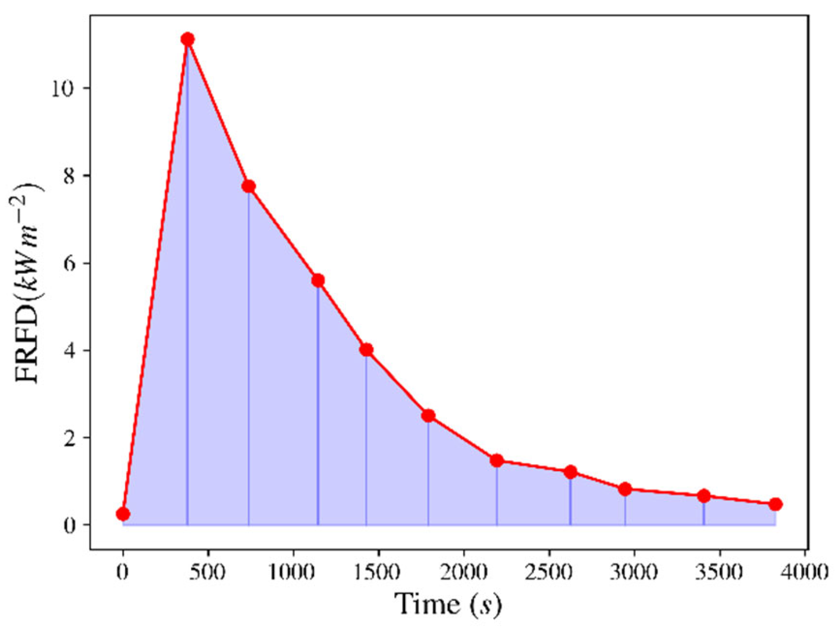
The integration of the radiative flux density with time, as depicted in
Figure 1, provides the fire radiative energy density (
FRED) [
14,
15,
16], a measure of the total radiative energy emitted from the fire environment, including flames, heated fuel elements, and the hot soil surface.
A time sequence of
FRFD can be used to calculate
FRED (Jm
−2) [
10,
11] based on Equation (2):
where
FRFDi is the
FRFD from each time sequence image
i, and
t is time.
Upwelling radiation from fires may be detected and has been measured using both satellite-based and airborne sensors [
11,
14,
15,
17]; the former give wide-area, infrequent coverage at relatively low resolution, while the latter provide potentially frequent, high-resolution observations over more limited areas.
A drawback of satellite-based systems is the difficulty in separating contributions of radiation from sub-pixel areas of unburned and burned ground or discriminating extensive sub-pixel areas of low-intensity combustion from smaller areas of high-intensity burning [
11]. Higher-resolution satellite-based sensors (e.g., Landsat8 OLI, Ball Aerospace, Broomfield, CO, USA) will also saturate over high-radiance fire targets, yielding artificially low radiance and temperature estimates. Lower-resolution sensors may avoid saturation by diluting the high-temperature signal with uncertain amounts of radiation from unburned or cooled ground [
14].
FRED, nonetheless, has been estimated based on satellite imagery [
14,
15].
Time-sequential, airborne thermal-infrared (ATIR) sensors have been used to monitor wildfire temperatures and progression [
11], estimate rates of spread across time intervals of a few minutes [
18], and estimate the radiant energy flux from fires over time [
11,
19]. Energy measurements have required specialized imagers that accommodate the very high radiances associated with wildland fires [
11]. For example, the USDA Forest Service Pacific Southwest Research Station (PSW) and Space Instruments, Inc. (Encinitas, CA, USA) co-developed the FireMapper and FireMapper 2.0 (FM2) imagers, which employ microbolometer focal-plane arrays with band-pass filters, to provide unsaturated fire measurements at thermal-infrared wavelengths of approximately 9 and 12 μm [
11].
Using repeat-pass imagery collected using FireMapper sensors from chaparral wildfires, Riggan et al. [
11] noted that there is often a qualitative and local spatial association of peak fire radiance with pre-fire biomass. Hudak et al. [
19] examined FireMapper imagery collected by PSW, over a burnout operation on the perimeter of the 2003 Cooney Ridge wildfire in Montana, and compared
FRFD and
FRED estimates from remote sensing with those derived from temperature measurements at the ground.
FRED has also been estimated from ATIR imagery collected over prescribed fires including the 2011 and 2012 RxCADRE experiments [
10,
17]. In the latter, the total fire radiant energy was four times higher from a forested plot than from one composed of dry grass, because of differences in fuel load [
10,
18]. Results from RxCADRE also highlighted the influence of the rate of spread and residence time on
FRED estimates. If a fire spreads rapidly with low residence time relative to the ATIR imaging frequency, some areas of active burning may not be imaged, yielding underestimates of
FRED [
20].
Controlled experiments like RxCADRE and the Cooney Ridge fire measurements implemented repeated ATIR imaging to estimate and map the intensity of relatively controlled and small-scale fires [
10,
18]. However, such observations of fire dynamics for small-scale experimental fires may not be representative of actively progressing, high-intensity, large-scale wildfires.
For this study, we assess procedures and their sensitivity when estimating FRED for the 2017 Thomas Fire in southern California, a rapidly expanding, large wildfire that burned primarily in chaparral during dry, Santa Ana weather conditions, and examine the spatial distribution of FRED. In the context of the Thomas Fire, we address the following research questions:
How sensitive are FRED estimates to the choice of ambient surface temperature, variations in FRFD time series shape, and incorporation of an adjustment for ash and char heating?
How do the magnitudes and spatial distributions of FRED vary for windy and less-windy wildfire spread conditions?
How does the spatial distribution of FRED co-vary with wildfire ROS?
2. Data and Methods
2.1. Study Area and Wildfire Context
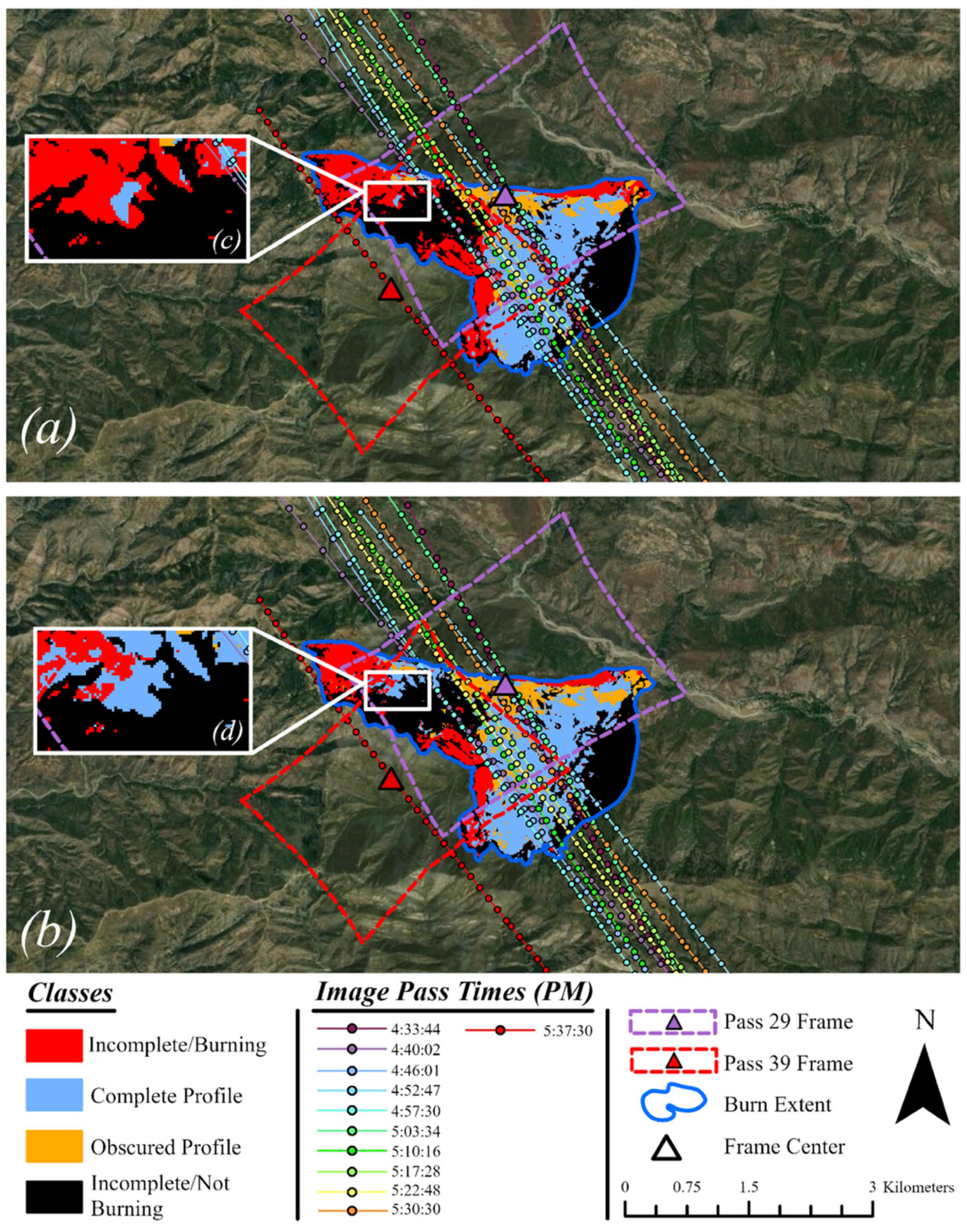
The study area consists of portions of the Thomas Fire that were imaged repetitively using an ATIR system on 8 December (Sequences 1 and 2) and 9 December 2017 (Sequence 3) [
18], provided in
Figure 2. The Thomas Fire burned from 4 December 2017 to 18 January 2018 across Santa Barbara and Ventura Counties, California, USA. At the time, it was the largest wildfire in Californian history. It mostly burned shrubby fuels in dense chaparral, with some subshrubs and grass fuels within coastal sage scrubs and trees, as well as herbaceous fuels of riparian and oak woodland communities also burning. The topography of the Thomas Fire burn extent is complex, consisting of hilly and mountainous terrain. The sequences for both dates were captured when the Thomas Fire was mostly spreading upslope [
18]. Sustained wind speeds during a Santa Ana (low humidity, high wind speeds) weather condition were estimated with the FireBuster model [
21], ranging from 1.3 to 1.8 ms
−1 for 8 December and 6.7 to 8.9 ms
−1 for 9 December [
18].
2.2. Image Data
We used time sequences of ATIR images of the Thomas Fire to estimate and analyze
FRED distributions for the Thomas Fire. An FM2 imager owned and operated by Kolob Canyon Aerial Services was flown on their Aero Commander twin-propeller aircraft. Most of the imagery was captured using a racetrack pattern, with the imaging flightline oriented perpendicular to the predominant fire spread direction and the active fire front within image frame coverage. The FM2 imager uses a microbolometer frame-based imaging sensor that measures thermal-infrared radiation, without requiring cryogenic cooling, and typically does not saturate [
11]. The FM2 sensor captured TIR radiance with a broadband (8.0–12.5 μ) and two narrowband (centered at 8.95 μ and 11.86 μ) channels, typical for land surface temperatures emissions. For this study, we exclusively used the IR3 narrowband, centered at 11.86 μ. The spatial resolution of the FM images varies as a function of altitude above ground level and was 10.4 m for the 8 December imaging sequences and 11.4 m for the 9 December sequence. The temporal resolution of the imagery is determined by the time between passes, which is determined by the ground speed of the aircraft flying and the size of the racetrack flight pattern [
18].
Table 1 contains image acquisition details for the three sequences.
FM2 images were georeferenced and orthorectified by USFS PSW, using Agisoft Metashape software (Version 1.8.4). Mosaics of the image frames were created using the maximum pixel value for overlapping orthoimages. Images were converted from digital number values to at-sensor radiances using a blackbody calibration curve with a radiance offset to control sensor drift that is caused by small changes in sensor temperature during imagery collection. Atmospheric correction was not applied to the imagery. Images were converted from radiances to apparent temperature values (in Kelvin).
2.3. General Methodological Approach
We assessed the sensitivity of FRED estimates to the selection of inputs and the spatial distribution of FRED for different weather conditions during the Thomas Fire, including ambient temperatures, a temperature adjustment associated with heating of ash and char surfaces, and atmospheric obscurations causing missing or attenuated FRFD values. We also characterized FRFD temporal trajectories using exponential decay functions and compared exponential decay coefficients for differing fire behaviors. Sensitivity and temporal profile analyses were based on repetitive FM2 image data for 9 December 2017 only. We estimated and compared FRED distributions and analyzed the spatial association between FRED and ROS for both the 08 and 09 December 2017 datasets.
The calibrated surface temperatures were processed to estimate
FRFD in MJm
−2 and
FRED in kWm
−2, based on Equations (2) and (3) [
19]. The time intervals used to estimate
FRED estimations were based on the recorded FM2 acquisition times for sequential images.
2.4. Ambient Temperature Selection
Since FRFD is derived from the difference between the burning and ambient (adjacent, non-burning) apparent surface temperatures, we evaluated the sensitivity of FRED estimates to ambient temperature selection. Ambient temperatures were estimated based on two sampling approaches, by extracting samples from several topographic aspect orientations for adjacent unburned areas and from a single long transect oriented traversing through a range of slope aspects and angles (and therefore, solar illumination conditions).
The slope aspect was derived using a USGS NED 10 m digital elevation model available through Google Earth Engine. The aspect raster was transformed and resampled to conform with FM2 pixels. Aspect was classified into the following four aspect classes: North (315° to 45°), East (45° to 135°), South (135° to 225°), and West (225° to 315°). Mean ambient temperature values across all image passes were calculated for pixels within each of the four slope aspect classes.
For the single transect approach, a 1.26 km transect was delineated across unburned vegetation adjacent to the burn scar and apparent temperature values were sampled for all pixels of the image time series. The criteria for delineating the transect included areas that did not burn throughout the duration of imagery and a line that transect a representative range in slope aspects orientations and, therefore, varying surface illumination conditions. The impact of ambient temperature uncertainty on FRFD and FRED was tested by estimating FRED and FRFD with a range of ambient temperatures. We used the minimum and maximum temperatures sampled (across all images) along the transect to determine the range of ambient temperatures.
2.5. Ash Temperature Adjustment
Due to the high emissivity and brightness temperature and low albedo of deposited ash and char during and immediately following smoldering combustion, the warmer background may erroneously contribute to
FRED estimation [
11,
22]. An alternative function to control for ash depositions during low temperature smoldering is defined as follows:
where
Ta is the temperature of ash in direct sunlight postfire, which was estimated by Riggan et al. [
23] to be 343 K.
The ash adjustment was applied for the portion of the
FRFD temporal profile when
Tf < 473 K, where 473 K was deemed to be the minimum temperature for chaparral to ignite based on the work of Engstrom et al. [
24]. Temperatures below this threshold were assumed to be associated with smoldering combustion and not flaming combustion. The adjustment was not applied for temperatures > 473 K, the temperature at which Riggan et al. [
11] found that flaming combustion is the predominant influence on TIR radiance, such that radiant energy from solar-heated ash radiance is negligible.
To evaluate the impact of applying an ash adjustment, we compared ash-adjusted with non-ash-adjusted FRED estimates. The ash- and non-ash-adjusted estimates were based on an initial ambient temperature of 289 K. Percent change in mean and median FRED was estimated, as well as percent change in the mean FRED for the highest intensity fires (95th percentile).
2.6. Temporal Profile Analyses
2.6.1. Profile Classification
Binary classifiers were implemented to characterize
FRFD temporal profiles, facilitating the selection of the most complete samples for analyzing peak
FRFD, decay coefficient estimation, and atmospheric obscuration adjustments. Pixels were classified sequentially into four classes, in the following order: Unburned, Burned, Complete, and Obscured, based on the rule sets shown in
Table 2. The minimum ignition temperature of chaparral, 473 K [
25], was used as the threshold temperature for the Burned classifier. Pixels were classified as Complete when subsequent images provided negligible increases in total
FRED and were classified as Obscured when there is a 40% increase in
FRFD after the onset of exponential
FRFD decay. A threshold of 40% was chosen based on empirical observations of
FRFD temporal profiles. Pixels classified as Burned were further classified as Incomplete or Complete, while pixels classified as Complete were further classified as Obscured or not Obscured. Ash and non-ash adjusted profiles were classified to identify variations in their temporal shape.
2.6.2. Peak FRFD Analysis
Hudak et al. [
10] noted the importance of capturing the peak
FRFD within a time series to accurately estimate
FRED. Peak
FRFD are associated with the zone behind the active fire front. They comprise a large proportion of the total energy density and not capturing the peak can lead to a substantial underestimation of
FRED. To assess the importance of peak
FRFD on estimated
FRED, we estimated the peak
FRED (
FREDpeak) as follows:
where
FREDpeak is the partial
FRED associated with the peak
FRFD,
tpostΔ is the time change (in seconds) between the peak
FRFD and the next image,
tpreΔ is the time change between the image prior to the peak and the peak
FRFD,
is the mean change in time, and
FRFDpeak is the maximum
FRFD in the temporal profile. Percent attribution of the
FRFDpeak to the cumulative
FRED is not possible without converting from flux density (Watts) to energy density (Joules).
FREDpeak was calculated for all profiles that were classified as Complete. To reduce the processing times of our analysis, peak
FRFD and cumulative
FRED were analyzed for profiles that peaked at image pass 2.
We also calculated FRFD over shorter time intervals and determined what percentage of FRED was contributed to by specific time segments. For a hypothetical FRFD temporal profile, 60% of the FRED was accumulated 40 min post-peak and 90% 56 min post-peak.
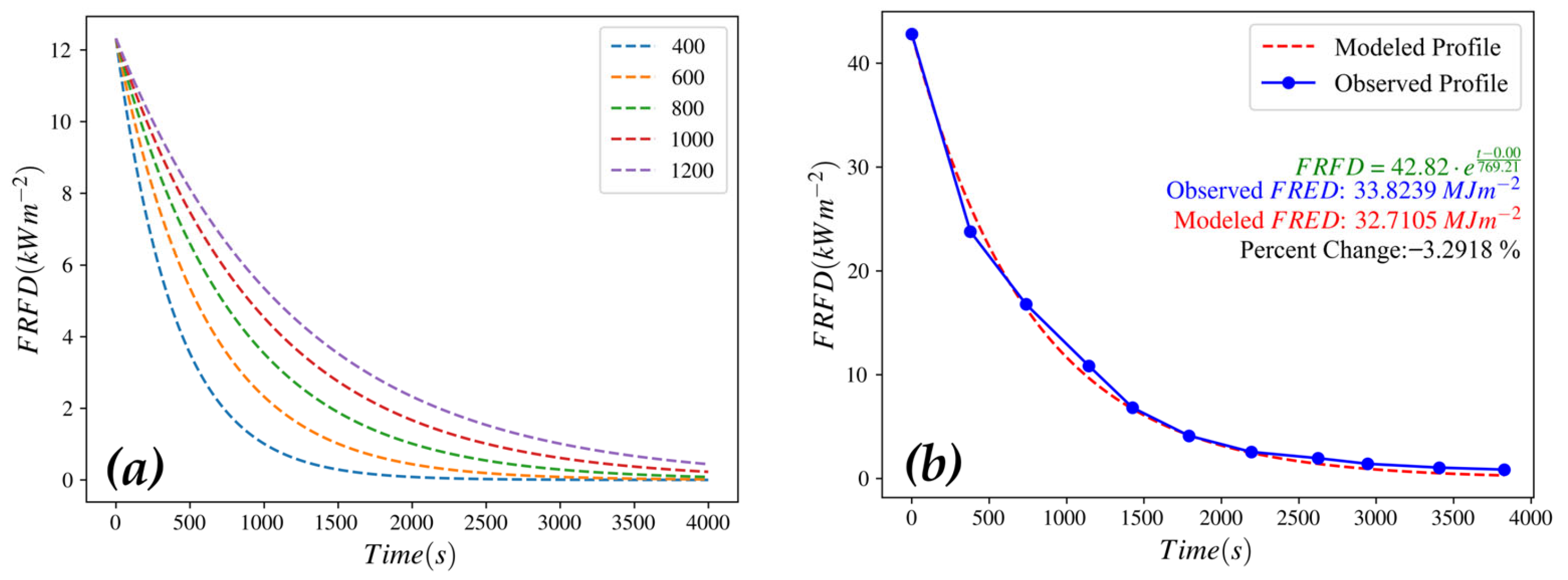
2.6.3. Exponential Decay Coefficients
Based on the general temporal temperature progressions of fires [
26] and empirical observations of temporal progression of
FRFD reconstructed from FM2 imagery,
FRFD profiles exhibit an exponential decay shape following peak burn temperature. Thus, the post-peak profile of
FRFD progression can be approximated using the following exponential decay equation:
where
A is the peak
FRFD (amplitude/
FRFD at ignition) (kWm
−2),
c is the time at ignition (s),
t is the time post-ignition (s), and
b is the exponential decay coefficient, commonly referred to as the half-life.
We assumed that the peak
FRFD (
FRFDmax) occurs the first time a pixel is imaged burning, when solving for the exponential decay coefficient (rate) (
b) using ordinary least squares regression. Both ash- and non-ash-adjusted profiles were regressed.
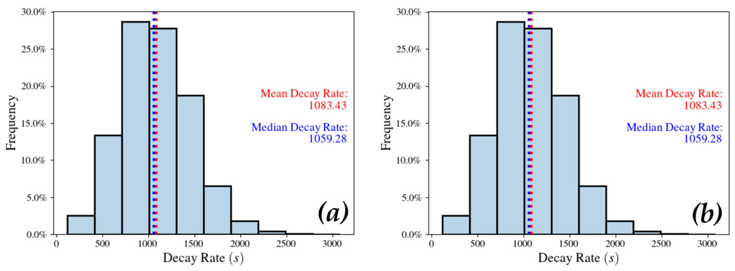
Figure 3 shows the steepness of the exponential decay curves with varying exponential decay coefficients and a sample outcome for decay function fitting. The decay coefficient was used as a metric for comparison, such as for determining the sensitivity of
FRED estimates to the use of ash adjustments. Decay coefficients were only calculated for pixels classified as Complete and not as Obscured. Maximum and minimum decay coefficients were also calculated to establish a range of decay coefficients. The mean and median decay coefficient for the 95th percentile of
FRED was calculated to approximate the temporal characteristics of the highest intensity fires.
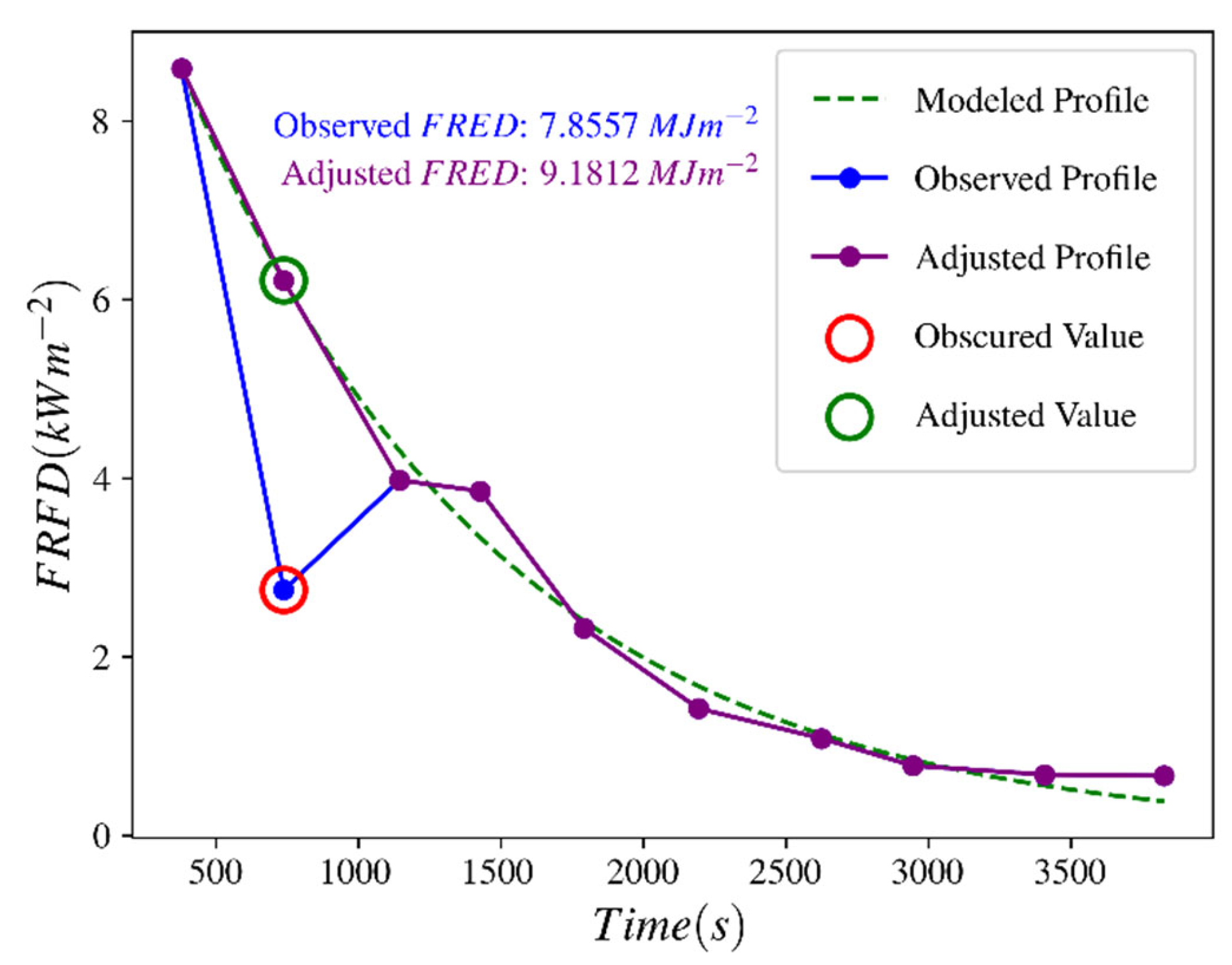
2.6.4. Obscuration Adjustment
Atmospheric obscuration from high water vapor concentrations or pyrocumulus clouds occurring during imaging of the Thomas Fire represented within
FRFD temporal profiles likely leads to the underestimation of
FRED [
11]. Despite these obscurations, profiles still exhibit exponential decay post-peak, when
FRFDpeak is not obscured. To adjust for obscuration, we fit exponential decay functions to the
FRFD temporal profiles classified as obscured and replaced the obscured
FRFD values with that estimated by the exponential decay models for the same time step. Obscuration adjustments were applied to both ash- and non-ash-adjusted temporal profiles.
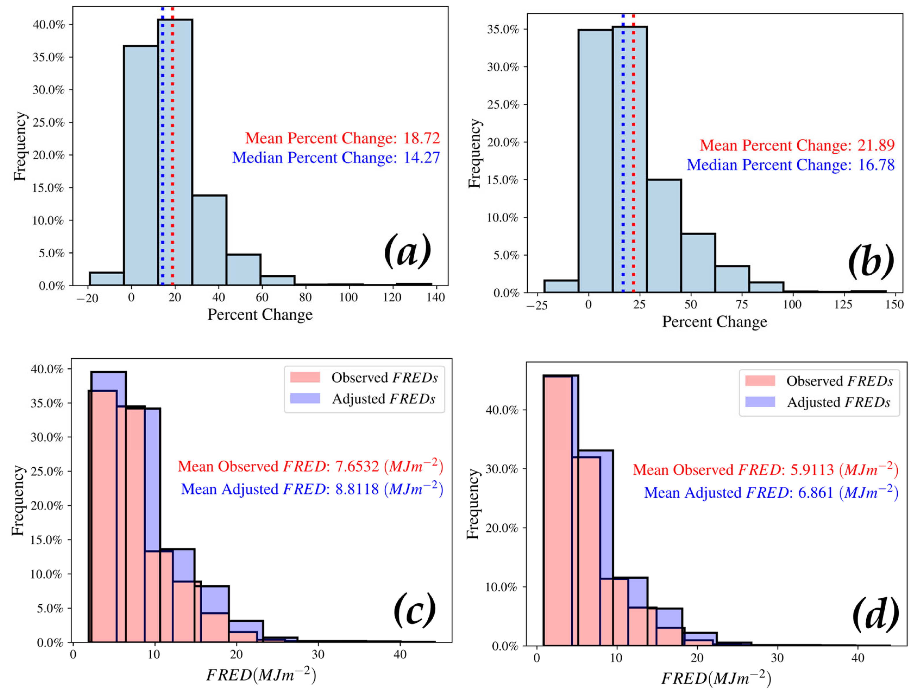
Figure 4 illustrates the obscuration adjustment approach carried out by filling in the obscured gap with the modeled value. To approximate the effectiveness of adjusting for atmospheric obscurations, we calculated the mean
FRED for all obscured profiles prior to adjustment. The mean
FRED and percent difference were calculated for the adjusted temporal profiles and were compared with the
FRED estimates based on unadjusted profiles.
2.7. Spatial Distribution of FRED Estimates
We analyzed
FRED magnitudes and spatial distributions, as well as the relationship of
FRED with wind speed and
ROS for the 8 December and 9 December ATIR sequences. An ambient temperature of 289 K was used for both dates. All pixels classified as Complete and not Obscured were compared between the two dates. To compare estimates between areas where active fire progression was observed,
FRED,
FRFD, and classification statistics were derived for samples adjacent to fire fronts delineated by Schag et al. [
20].
We generated and overlaid grid cells larger than the ground sampling distance of FM2 imagery, to sample
FRFD and
FRED estimates for comparison with the
ROS estimates made by Schag et al. [
20], to facilitate analysis of
ROS and fire intensity relationships. Two grid cell sizes were tested, as follows: 22.75 m × 22.75 m (2 × 2 pixels) and a 34.13 m × 34.13 m (3 × 3) grid. Mean temperature and
FRFD values were calculated for each grid cell using zonal statistics in ArcGIS Pro. Grid cell sampling was restricted to non-ash-adjusted
FRFD. Centroids of ROS vectors were assigned a 2 × 2 and 3 × 3 grid cell, using a spatial join in ArcGIS Pro. We ran an ordinary least squared regression to compare assigned
FRED and
ROS for grid cells.
Previous studies by Riggan et al. [
11] and Hudak et al. [
10,
19] highlighted the importance of pixel proximity to fire front location during image sampling. Higher
FRFD and
FRED were observed near the flaming front’s location during imagery collection. To assess the impact of fire front proximity to measured
FREDs and
FRFDs, we identified four locations (two for 8 December and two for 9 December) across fire fronts delineated by Schag et al. [
18]. Criteria for fire front locations were based on the frequency of Complete and not Obscured pixels within 250 m of the fire front. For each of these four locations, we drew buffers extending 225 m away from the fire front location, with each buffer having a width of 25 m.
2.8. Toolsets and Software
Modules for FRFD and FRED estimation and pixel classification were developed in Python 3.10, using the GDAL and rasterio python libraries. Exponential decay coefficients were approximated using the curve fitting function from the SciPy python library. Sampling grids were created using the OGR and geopandas python libraries, and a zonal statistics tool in ArcGIS Pro was used to select FRFD samples. A transect for ambient temperatures was delineated and sampled using a custom GIS GUI developed in Python 3.10, built with the folium and PyQT5 libraries. All graphs and plots were created using the matplotlib python library. All Python code is available on GitHub as an ArcGIS Pro Python Toolbox (Version 3.9).
4. Discussion
Studies pertaining to the estimation and analysis of fire intensity metrics, such as
FRED, based on repetitive ATIR imaging have primarily been conducted during controlled experiments, including the RxCADRE [
10,
17] and Cooney Ridge campaigns [
19]. Other studies have used multi-temporal satellite image data with low spatial and temporal resolution [
27,
28,
29]. A notable gap in the literature exists for fire intensity estimation at landscape-scales using ATIR imagery. The main research objectives of this study were to determine the procedural approaches and their sensitivities for the reliable estimation of
FRED using time sequential ATIR image data for 9 December (Sequence 3), and to assess how
FRED varies spatially and in comparison with ROS for both 8 December and 9 image sequences captured during the Thomas Fire.
The outcomes of this research add to findings of Boschetti and Roy [
27] and Hudak et al. [
10,
19] by bridging the gap between small-scale, experimental studies to a landscape-scale study of a free-burning wildfire. We developed new methods and tools to address the implications of atmospheric obscuration, ash radiances, and co-registration errors to improve the reliability of
FRED calculations. We also developed methods for properly characterizing
FRFD temporal profiles (through classification and function fitting) to help improve imagery collection, processing, and analysis in the future. This work builds upon the works of Schag et al. [
20] by exploiting ATIR image sequences for estimating fire ROS and assessing its covariation with
FRED.
4.1. Sensitivity of FRFD and FRED Estimation Procedures
While ground-based systems for ambient temperature determination were employed in fire intensity studies based on experimental fires [
10,
19], our results indicate that an image-based approximation of ambient temperatures is suitable for estimating
FRED. Controlling for variations in slope aspect illumination were found to be not important unless the difference in illumination leads to a substantial difference in surface temperatures (>30 K). Lower
FRFD estimates resulting from higher ambient temperatures were most apparent near the end of
FRFD temporal profiles, where surfaces reach temperatures < 400 K and begin to level off. However, this had little impact on
FRED estimates due to >90% of the energy density being accumulated prior. More reliable ambient temperature determination may be required for studies focused on low temperature smoldering combustion.
Riggan et al. [
11] noted the low impact of ash depositions during flaming combustion, so a background adjustment for ash depositions was deemed unnecessary for their fire intensity estimation. However, in this study,
FRFD for low temperature smoldering combustion was found to be influenced by radiance from heated ash, such that applying an ash adjustment led to a substantial difference in the
FRFD temporal profile shape and accumulated
FRED. The end of the
FRFD temporal profile dips substantially for ash-temperature-adjusted profiles compared to those using ambient temperature subtraction. When compared to non-ash-adjusted profiles, the application of the ash adjustment led to a lower
FRED estimate, a greater number of Completed and Obscured profiles, a greater impact of the peak
FRFD on
FRED, and steeper exponential decay models. Ash adjustments applied to
FRFD profiles were based on values from a previous study conducted in a tropical savanna [
11]. Other approaches could include controls for slope aspect due to variations in solar irradiance [
11], or controls for varying ash colors [
23]. High-intensity fires deposit a thick layer of white/gray ash, while low-intensity fires consume less vegetation and leave a dark (gray or black) ash layer [
23]. These variations in ash layer color affect the solar absorption and emitted radiance of surfaces, such that a characterization of ash background temperature based on fire intensity (e.g., peak
FRFD) may be a useful indicator of ash radiances during smoldering combustion [
23].
Hudak et al. [
10,
19] noted the importance of sampling the peak temperature within the temporal profile, since a large portion of the estimated energy density is attributed to the peak. While capturing the peak temperature of the temporal profile is key to reliably estimating the total energy density, we found that the degree to which the total energy density is attributed to the peak temperature is highly variable. For example, the peak temperature contributed > 60% of the measured
FRED for some temporal profiles and as low as 20% for others. Achieving an adequate sampling frequency is key to capturing the peak temperature, but the duration of sampling is also important for properly estimating
FRED.
Another important consideration regarding capturing the peak temperature of the temporal
FRFD profile is that the maximum recorded temperature may not represent the true peak temperature. This may occur because a pixel during a TIR image pass was not sensed at or near the passing of the active fire front, or because of the relatively low emissivity values associated flames, which are gray body radiators [
9,
15]. The latter means that the true “peak” for a temperature temporal profile may be underestimated, unless the emissivity of the flaming zone was known and used to modify surface temperature estimates. Riggan et al. [
11] proposed a multiband method to adjust for surface emissivity, but such a method is not feasible for the single, narrow-band TIR data utilized for this study.
FRFD temporal profiles were numerically characterized using an exponential decay model, particularly through the exponential decay coefficient. While Hudak et al. [
10,
19] noted the exponential decay shape of
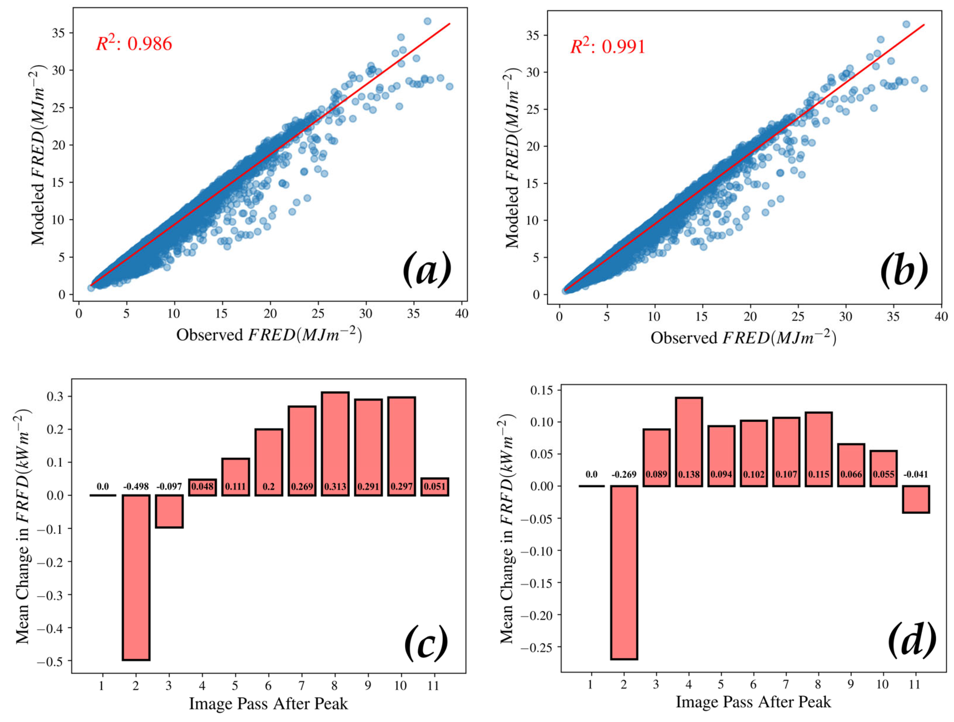
FRFD temporal profiles for the RxCADRE and Cooney Ridge experiments, no metric was utilized to quantify the form of the profiles. Modeled and observed
FRED estimates in this study are highly correlated (R
2 > 0.98 for both ash- and non-ash-adjusted), providing a proxy measurement for the accuracy of decay function fit. Alexander [
26] reported temperature temporal profiles exhibiting a similar exponential decay shape, which support the reliability of our findings. Despite the high degree of fit with modeled
FRED, residuals between the modeled and observed
FRFD values are greater for
FRFD measurements later in the time series. This may result from the exponential decay function being strongly influenced by the peak amplitude, a parameter that is not calculated through least squared regression.
We demonstrated that atmospheric obscuration is a source of missing or reduced surface temperature observations for ATIR imaging of active fires [
11], which influences the ability to adequately sample
FRFD for
FRED estimation. Riggan and Tissell [
11] state that pyrocumulus clouds and water vapor produced by flaming combustion can obscure radiances within the TIR spectral range (8–12 um). Our obscuration classification results suggest that obscuration was not common for the passes over the Thomas Fire incorporated in this study, though obscuration associated with the high-intensity, rapidly spreading fire captured during Sequence 3 was evident.
Other studies concerned with the estimation of
FRED based on ATIR imaging have not identified or adjusted for obscured pixels in temporal profiles, possibly because they were based on experimental burns that do no generate large plumes of water vapor and/or pyrocumulus clouds [
10,
17,
19]. By identifying obscured pixels and fitting an exponential decay function to temporal
FRFD profiles, obscured values can be adjusted and associated energy density losses can be compensated.
In some instances, poor exponential decay model fits or poorly identified obscured profiles lead to unreliable FRED estimates. This stemmed from errors in classifying obscured profiles, where small variations in measured FRFD during smoldering combustion (when the temporal profile flattens out) were identified as an obscuration. Based on FRFD residuals results from Complete and non-Obscured profiles, modeled FRFD values later in the time series were lower than observed FRFD. Since Obscured values in the temporal profile occurred later in the time series, the modeled FRFD was lower.
Exponential decay function fitting was shown to be a useful alternative to commonly used gap-filling or anomaly smoothing methods to account for gaps caused by Obscured values, such as Savitzky–Golay or Whitaker filtering [
24]. Future applications of the exponential decay function may include value predictions later in the time series. If the decay coefficient from an
FRFD temporal profile can be determined based on an incomplete temporal sequence, particularly with a few key clear images captured near the start of the time sequence, the distance decay modeled shape may be sufficient for reliably estimating
FRED.
4.2. FRED Distributions and Relationships
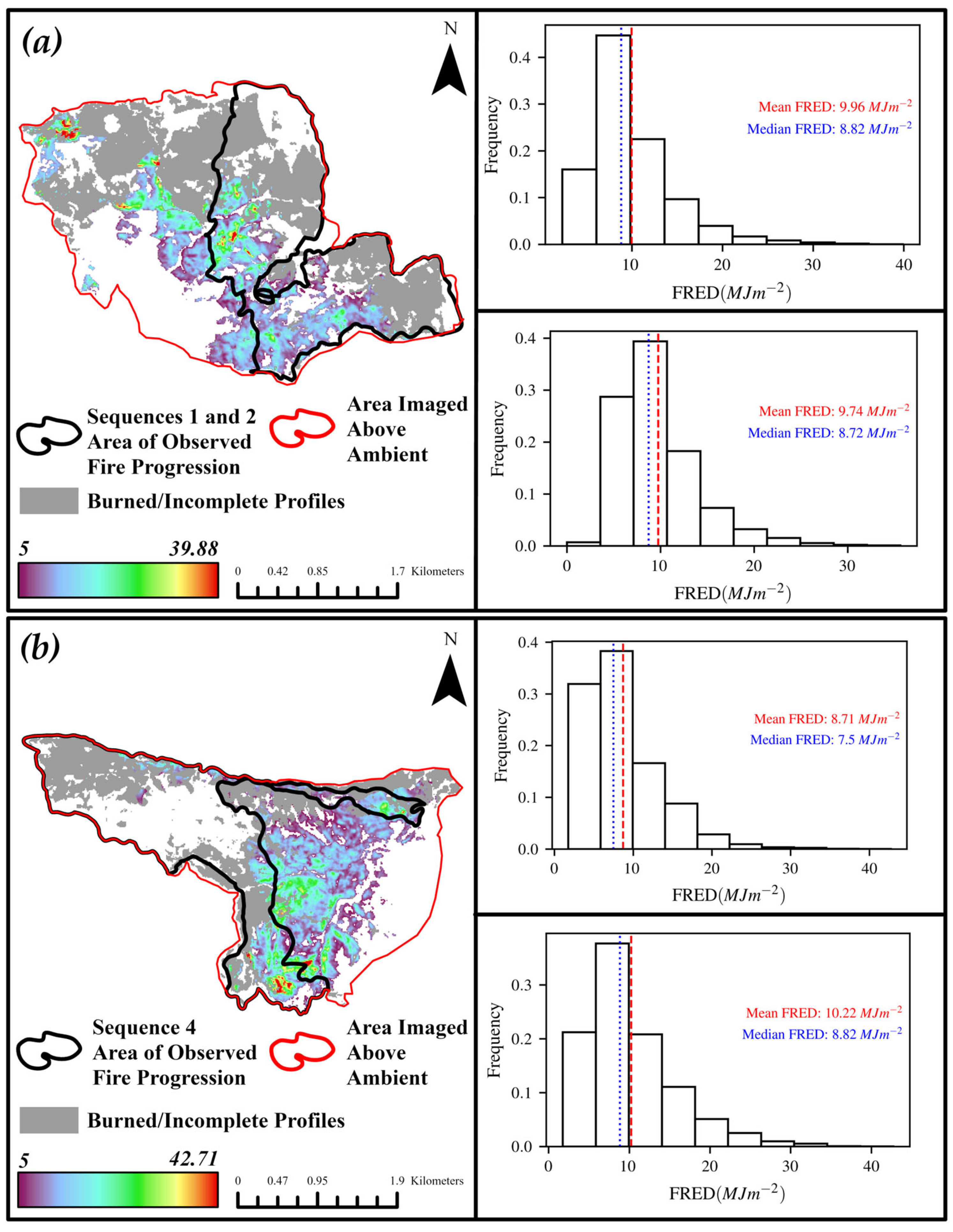
When including the entire burn extent captured by repetitive ATIR imaging, which includes spot fires and stagnating fire fronts,
FRED magnitudes were estimated to be higher for the 8 December passes that burned during moderate wind speed conditions than for the 9 December passes. After restricting sampled pixels to the fire front area (where fire progression is active),
FRED and peak
FRFD statistics are higher on 9 December than 8 December. The Rothermel model of fire propagation includes reaction intensity (Wm
−2) as a variable that increases
ROS, so a higher
ROS may be associated with a higher intensity heat source [
30]. Therefore, peak
FRFD statistics may be a helpful approximator for fire rate of spread.
Despite the higher estimated cumulative fire intensities for 9 December, the frequency at which pixels were imaged burning was lower. Only 50% of pixels within the fire area were classified as Burning for 9 December, while 70% were classified as Burning for 8 December. This is likely due to active fire progression being fast relative to the repetitive imaging frequency for 9 December, preventing the flaming combustion to be captured during image passes. This is emphasized by a large extent, seen in
Figure 11b, with a lack of pixels classified as Burned within the active fire front zones imaged at that time.
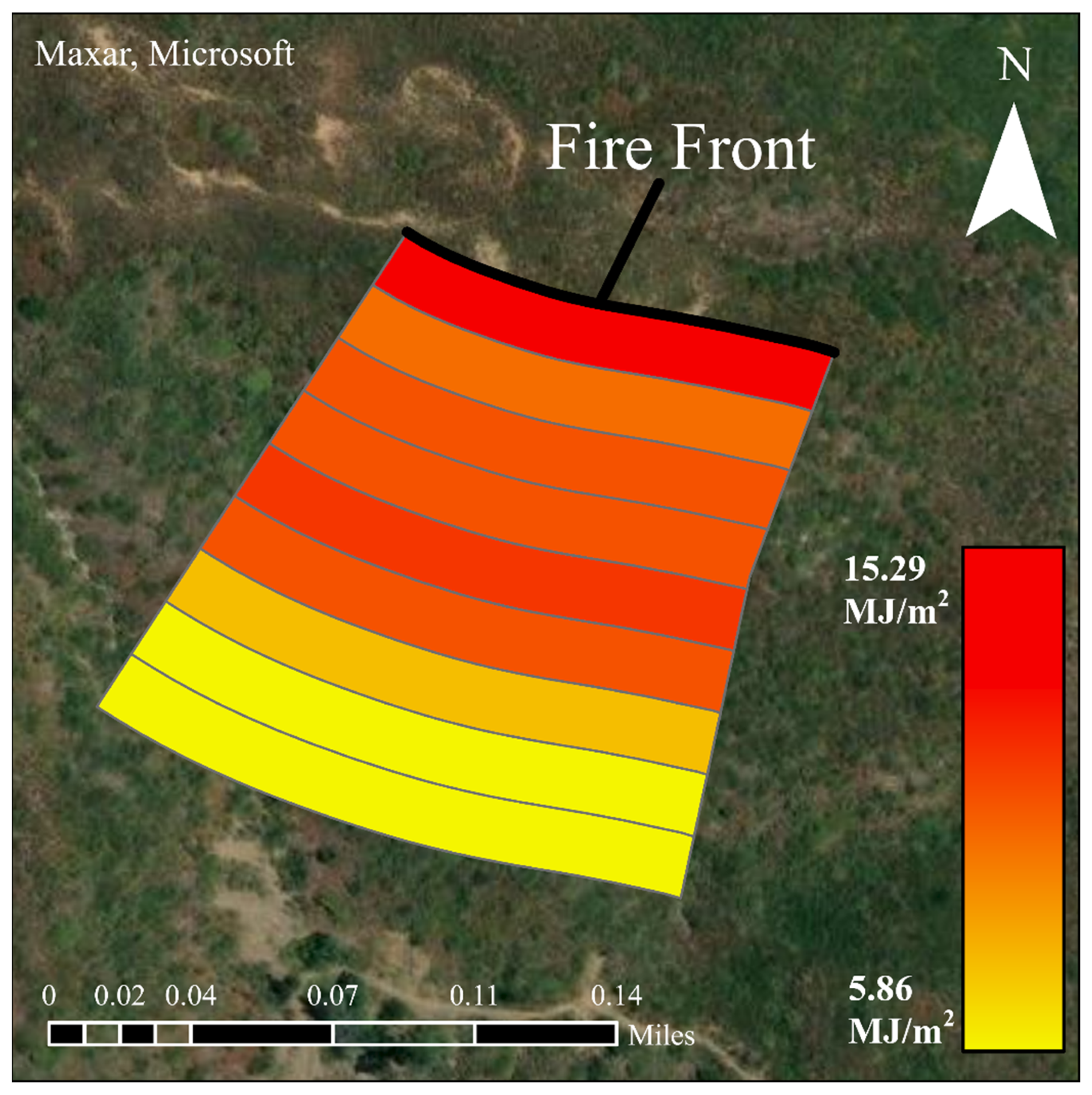
Spatial distributions of estimated fire intensity in previous studies by Hudak et al. [
10] and Riggan et al. [
11] indicated that the higher fire intensities were located near the actively progressing head. Using our buffer approach, such an association is not evident in our
FRED estimates. However, the progressive decrease in measured
FRED as the buffer distance increases may provide an indication of an ideal zone for
FRED estimation.
Maps depicting spatial distributions of
FRED can be important datasets for studying fire behavior and the impacts of
FRED on burn severity and postfire recovery. For example, Hudak et al. [
19] found that ash deposition postfire was positively correlated with measured energy densities during the Cooney Ridge Fire Experiment. Ash deposition influences could be compared by using a coarse grid to sample Landsat-derived NBR/dNBR.
FRED distributions could also be examined relative to distributions of postfire recovery trajectories, such as those derived from Landsat time series. [
31,
32,
33].
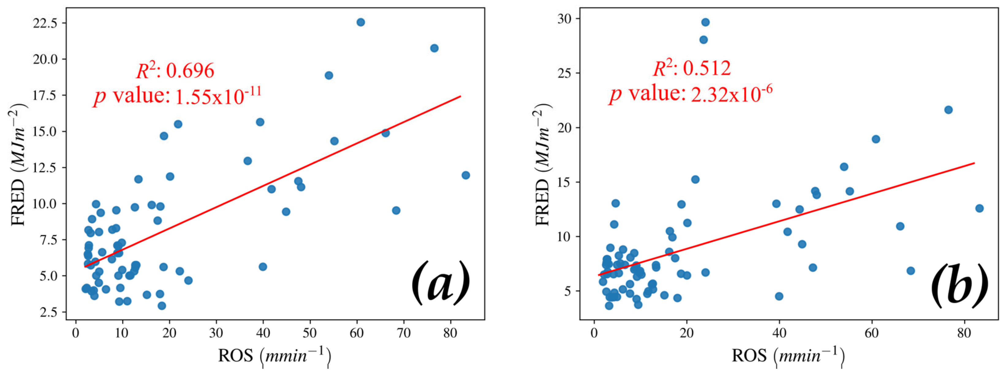
Results from this thesis research indicate that ROS is positively correlated with
FRED for burned areas of the Thomas Fire where adequate temporal sampling of ATIR-derived brightness temperatures was achieved. The spatial extent of the sampled area was limited due to a lack of Complete and non-Obscured profiles spatially associated with
ROS vectors. The application of decay coefficients for completing incomplete profiles is useful for gap filling and increasing the number of samples for
ROS and
FRED analysis. Portions of the active fire where
ROS was estimated to be spreading fastest (95th percentile of spread vectors) were not included in the sample since they were not classified as Burned or Complete. This is consistent with the observation of Hudak et al. [
10] that when
ROS is high, flaming combustion may not be imaged for many locations, leading to an underestimation of
FRED for those locations [
10].
5. Conclusions
This study addresses procedures and their sensitivity and reliability for reconstructing time sequences of TIR flux densities and estimating
FRED for active wildland fires through aerial thermal-infrared imagery at a landscape scale, a shift away from previous studies that calculated
FRFD and
FRED through controlled experiments [
10,
19]. We addressed the impact of ambient temperature approximations on fire intensity measurements and conclude that variable approximations of ambient temperature do not impact the discrimination of high- and low-intensity fires. We provided an alternative approach to background temperature subtraction that controls ash radiances during low temperature smoldering combustion. Using the fire temperature time series developed by Alexander [
26] as a reference, we developed and fit an exponential decay model to
FRFD temporal profiles to properly characterize how flux densities decay over time. We used these decay models to adjust for classified instances of obscuration within
FRFD temporal profiles.
ROS vectors and
FRED comparisons between 8 and 9 December 2017 imaging passes for the Thomas Fire provide an indication of how
ROS covaries with
FRED.
While the outcomes from this study are promising, some challenges and limitations were faced when conducting the research. First, the imagery for this study was originally used for ROS research. The racetrack flight method makes it possible for repeat passes to be consistent and fast; however, the tracking of numerous flaming fronts can extend the return interval. The tradeoff for a longer return interval is providing a larger area of coverage. This leads to a tradeoff researchers must consider; the return interval can be decreased by focusing on a smaller area (individual front), but coverage is limited. A fast
ROS and long return interval may prevent imaging during peak combustion. As previously mentioned, variations in surface emissivity and obscurations provide a level of uncertainty in estimating
FRED [
11].
Future studies should consider the refinement of flight patterns and repeat frequency when collecting ATIR imagery. While the sampling duration is important for accurate approximations of FRED, a higher sampling frequency would increase the likelihood of collecting the peak and provide more samples for FRFD temporal profiles. A racetrack flight pattern that covers a small area would increase the sampling frequency and prevent mischaracterizations of FRED due to missing instances of flaming combustion, especially for fast-spreading fire fronts. The tradeoff for increasing the sampling frequency would be a reduction in spatial coverage.
Studies of cumulative fire intensity should be conducted with airborne sensors utilizing additional infrared wavebands. Riggan and Tissell [
11] noted the importance of using SWIR or MIR in conjunction with LWIR for accurate approximations of fire intensity. An appropriate research direction would be analyzing
FRED distributions relative to image-derived metrics for prefire fuel load and/or moisture and postfire burn severity maps derived from satellite spectral vegetation indices [
32]. Assessing spatial correspondence of
FRED relative to topographic variables such as directional slope [
18] would be another worthwhile objective. Fuel loads and moisture in southern California chaparral vary based on slope aspect, specifically northern- and southern-facing slopes [
34]. Southern slopes are less dense with vegetation than northern-facing slopes [
34], so spatial distributions of
FRED may reflect topographic differences across landscapes.


 ,
, 


