Fire Source Determination Method for Underground Commercial Streets Based on Perception Data and Machine Learning

Abstract

Determining fire source in underground commercial street fires is critical for fire analysis. This paper proposes a method based on temperature and machine learning to determine information about fire source in underground commercial street fires. Data was obtained through consolidated fire and smoke transport (CFAST) software, and a fire database was established based on the sampling to ascertain fire scenarios. Temperature time series were chosen for feature processing, and three machine learning models for fire source determination were established: decision tree, random forest, and LightGBM. The results indicated that the trained models can determine fire source information based on processed features, achieving a precision exceeding 95%. Among these, the LightGBM model exhibited superior performance, with macro averages of precision, recall, and F₁ score being 99.01%, 98.45%, and 99.04%, respectively, and a kappa value of 98.81%. The proposed method for determining the fire source provides technical support for grasping the fire situation in underground commercial streets and has good application prospects.

1. Introduction

Since the “12th Five-Year Plan” period, the development and utilization of urban underground space in China have shown a trend of scale and growth, making China a vast country in developing and utilizing urban underground space [1]. In underground space development, underground commercial streets have rapidly expanded, relying on the vast pedestrian flow brought by rail transit, effectively alleviating urban land pressure, and promoting economic and social development. However, large-scale fires can quickly occur due to the complex internal structure, high personnel density, and flammable materials in underground commercial streets, causing severe economic losses or casualties [2].

Grasping the correct fire source information can help firefighting and rescue personnel to understand the development of the fire and to make correct firefighting decisions. When a fire occurs in above-ground buildings, the fire source location or fire development can be identified by observing the firelight and smoke outside the building. However, after a fire breaks out in an underground commercial street, the fire scenario cannot be directly observed, resulting in a lack of information during firefighting decision making, leading to incorrect judgments [3].

In the field of quantitative risk analysis (QRA), the determination of fire source information is crucial [4]. The identification of fire source information directly impacts the design of evacuation routes, the establishment of smoke propagation models, the optimization of emergency response resource allocation, and aspects of risk prediction and assessment. In the study and practice of fire risk analysis, it is imperative to develop efficient fire source identification technologies.

Many scholars have recently applied machine learning methods to predict fire parameters after a fire occurs. Machine learning is inputting a dataset from numerical simulation or loT devices into a model for training and testing, thus obtaining the coupling relationship of specified parameters in the dataset [5]. Machine learning algorithms can predict parameters by collecting data on fire parameters, such as temperature, smoke, and gas. Deng et al. [6] used three parameters to establish a gated recurrent unit (GRU) neural network model to predict the highest temperature of the tunnel ceiling. The results showed that the machine learning algorithm was consistent with the verification experiment. Saeed et al. [7] established a fire detection convolutional neural network model based on smoke and heat, which can effectively predict fires with an accuracy of 91%. Liu et al. [8] established a fire detection model based on six machine learning algorithms, such as logistic regression, among which the K-nearest neighbor algorithm demonstrated the best classification performance. Hodges et al. [9] predicted the temperature distribution in a room based on transposed convolutional neural networks; the prediction accuracy reached 95%. These studies selected appropriate feature parameters based on their predictive objectives and achieved relatively good prediction results.

Regarding fire source determination technologies, Yan et al. [10] proposed the use of the least squares method based on the Gaussian plume model for fire source localization and the application of the K-means clustering method to reduce localization errors. However, this technique requires the deployment of a large number of gas concentration sensors. Sun [11] introduced a method for fire source localization using distributed fiber optic temperature sensors, effectively measuring temperature and determining the fire source’s location, yet was unable to ascertain other key parameters like the heat release rate. Chu [12] et al. developed a fire source localization model based on computer vision, although it is limited to the detection and localization of fire sources. Shen [13] used thermal flux parameters to infer fire source diameter and heat release rate, however, thermal flux sensors are expensive and prone to failure. Zhang et al. [14,15,16] established a large tunnel fire database, creating a machine learning model that inputs temperature to predict tunnel fire source location, time of danger, and temperature field parameters. This method is cost-effective and relatively precise, yet it does not cover other key parameters of the fire source. However, previous studies have not applied machine learning algorithms that demonstrate good predictive performance to fire source determination in underground commercial streets, which is an area that requires further research.

In the study of information identification of fire source, existing AI fire determination models, such as OpenCV systems [12], Bayesian machine learning [13], and neural networks [16], show unique advantages and limitations compared to traditional fire source determination techniques like wireless sensor networks and distributed fiber optic temperature sensing systems. Traditional fire source determination methods, such as direct physical measurement and real-time monitoring, offer the advantages of accurate measurements and instant data on temperature and fire source location. However, these methods are limited by the spatial coverage of sensors and are costly in terms of maintenance and initial investment. On the other hand, existing AI models for fire source determination excel in handling complex data, automatically selecting influential features, enhancing predictive performance, and adapting to new data, making them suitable for dynamic fire scenarios. Nevertheless, these AI models face challenges in interpretability, especially complex ones like neural networks, and their performance is heavily dependent on the quality and representativeness of the data.

To address the issues of poor interpretability and data dependency in existing AI fire source determination models, this study proposed the establishment of machine learning models with strong interpretability, such as decision tree, random forest, and LightGBM models. To tackle the challenge of data dependency, it suggested creating a more realistic fire database through sampling to determine fire scenarios. Therefore, this study aimed to determine fire source information, like the specific location and heat release rate, via analyzing temperature time series. The study began by selecting fire scenarios using sampling, and simulating them with CFAST 7.7.4. software to build a database for underground commercial street fire scenarios. Subsequently, the obtained temperature was used for feature extraction and processing. Finally, the study developed and applied various machine learning models to accurately determine the fire source in underground commercial streets.

2. The Principle of Machine Learning Models

In machine learning, the objective of fire source classification is to allocate data to predefined fire source categories. The training involves learning the mapping relationship between data features and fire source categories. This paper established three machine learning models: decision tree (DT), random forest (RF), and LightGBM.

2.1. Decision Tree [17]

A decision tree builds a tree by recursively splitting the dataset. Each split is based on features that maximize the purity of fire source determination. The decision tree model in this study utilized the Gini index as the splitting criterion, selecting features and split points that significantly reduced uncertainty after the split.

The Gini index formula [18]:

$$Gini(D)=1-{\displaystyle {\sum }_{i=1}^m{p}_i^2}$$

(1)

Here, $D$ represents the established training set.

$m$ is the number of fire source categories.

$p_i$ is the proportion of samples of the $i$-th fire source category in the training set $D$.

For each split in the tree, the algorithm chooses the feature and split point that minimizes the Gini index of the child nodes. The reduction in the Gini index for a given node due to a split is defined as:

$$\Delta Gini(D,f)=Gini(D)-(\frac{\left|D_{left}\right|}{\left|D\right|}Gini\left(D_{left}\right)+\frac{\left|D_{right}\right|}{\left|D\right|}Gini\left(D_{right}\right))$$

(2)

Here, $f$ is the feature considered for splitting.

$D_{left}$ and $D_{right}$ are the two subsets of the dataset after the split.

$\left|D\right|$, $\left|D_{left}\right|$ and $\left|D_{right}\right|$ are the number of samples in the parent node and the two child nodes, respectively.

2.2. Random Forest [19]

Random forest is an ensemble learning method composed of multiple decision trees. Each tree is built independently, and randomness is introduced in the construction process. This randomness was achieved through Bootstrap sampling of the training data and selecting the best split from a random subset of features at each node. The random forest model can be represented as follows:

$$RF(x)=\mathit{model}\{D{T}_1(x),D{T}_2(x),\dots ,D{T}_n(x)\}$$

(3)

Here, $D{T}_i(x)$ refers to the output of the $i$-th decision tree.

$RF\left(x\right)$ refers to the output of the random forest, which was determined via aggregating the predictions of all trees through a voting mechanism for the classification of the fire source.

2.3. LightGBM

LightGBM is a gradient-boosting algorithm that iteratively adds a decision tree to minimize the loss function [20]. Each new tree in the algorithm was constructed to address the residual errors made by the previous trees in the sequence.

$$F_m\left(x\right)=F_{m-1}\left(x\right)+\alpha \cdot h_m\left(x\right)$$

(4)

Here, $F_m\left(x\right)$ represents the prediction of the model at the $m$-th step,

$h_m\left(x\right)$ is the prediction of the new tree added in that step,

$\alpha$ is the learning rate.

Distinct from the traditional gradient boosted decision trees (GBDT), LightGBM incorporates two primary technological advancements: histogram optimization and a leaf-wise growth strategy [21].

Histogram optimization: LightGBM constructs histograms by dispersing the values of continuous features into discrete bins, thereby reducing computational requirements.

Leaf-wise growth strategy: LightGBM opts to grow the leaf to maximize loss reduction, focusing more on minimizing the model’s error.

2.4. Application Examples

For instance, if the input features of the model are denoted as $x=\left(x_1,x_2\right)$, and the output fire source classification results are A, B, C, then a simplified decision tree may employ rules of the following form:

If $x_1>threshol{d}_1$, then:

If $x_2>threshol{d}_2$, then:

Classify as A;

Else

Classify as B;

Else

Classify as C.

In this example, $x_1$ and $x_2$ are features, and the thresholds determined how nodes were split. Random forest aggregates the results of multiple decision trees and decides the final classification through voting, while LightGBM iteratively optimizes each decision tree towards an optimal solution.

The model output $y$ is a function of the input vector $x$, which can be mathematically represented as follows:

$$y=f\left(x;\Theta \right)$$

(5)

where $f$ represents the model function, $\Theta$ is the parameters.

For the three established machine learning models, the input was a feature vector $x=\left(x_1,x_2,\dots ,x_n\right)$ processed from data, and the output was a fire source prediction classification based on the data distribution and structure learned by the model. In practical applications, the implementation and optimization of these models involve more details, including feature selection, model parameter adjustment, and overfitting prevention. Each model provides a fire source classification label for the input feature vector $x$.

3. Dataset Description

3.1. Introduction to CFAST

CFAST 7.7.4. is a dual-zone fire simulation software developed by the National Institute of Standards and Technology (NIST) [22]. When simulating with CFAST 7.7.4. software, the location of the fire is divided into an upper hot smoke gas zone and a lower cold air zone. The parameters in each zone are assumed to be uniform, and no diffusion and mixing of material across the interface between the two zones are considered. Using the CFAST software for fire simulation, the fire development status of multiple rooms, such as temperature and gas concentration as a function of time, can be obtained relatively quickly.

When using CFAST software for fire simulation, the simulation results are more accurate when the simulated space is smaller. However, for larger spaces, to make the simulation of the smoke movement more realistic, the simulated large space is usually divided into smaller sub-zones [23].

3.2. Introduction to CData

CData is a CFAST input data generator that creates one or multiple CFAST input files and creates batch processing programs [24]. This tool utilizes Monte Carlo sampling based on user-specified ranges and distributions of parameters to generate the input files for CFAST.

3.3. The Validity of the CFAST Model

NIST and many researchers have demonstrated the effectiveness of the CFAST model. Peacock et al. validated the CFAST model against fire phenomena in nuclear power plants, concluding that the simulated results of the temperature and height of the hot gas layer and oxygen and carbon dioxide concentrations were consistent with the experimental results [25]. Still, the smoke concentration tended to be overestimated. The delay of smoke propagation in corridors [26] and the chimney effect in shafts [27] were also validated against experimental data. Fan used CFAST to simulate fires in narrow and confined spaces, with a reasonable subdivision of sub-zones, and validated the simulation results [28].

3.4. Model Building

The research object was an underground commercial street with a length of 63 m, a width of 14 m, and a height of 4 m, encompassing a total construction area of 882 m² and a volume of 3528 m³. The street included a 4 m wide pedestrian passage in the center. On both sides of the pedestrian passage were 16 shops and 2 emergency exits, each with a length of 7 m and a width of 5 m. Temperature sensors were installed on the corridor’s ceiling in the underground commercial street.

3.4.1. Construction of CFAST Model

(1)

Geometric model.

The CFAST software demonstrates higher precision in simulating building fires in smaller spaces. However, its accuracy decreases with the increase in the size of the simulated space, leading to larger errors. To improve its efficacy for regional simulation of building fires, an enhancement of this simulation method is required. This refinement is crucial for achieving more accurate simulations across various spatial dimensions. Chow found that in the CFAST simulation of the tunnel fire, the simulation results of dividing the tunnel area into less than or equal to 15 sub-zones were scientifically effective [29]. The corridor area was uniformly divided into 9 sub-zones to create this fire model. Figure 1 below shows the CFAST model, with zones 1–16 as shops, 17–18 as emergency exits, and 19–27 as subdivided corridor sub-zones. The corridor area is demarcated by horizontal light-blue dashed lines. The fire source determination conducted in this study was solely for validating the proposed method. Therefore, fire sources were set in room 1, 2, 3, 4 and 5 in the CFAST simulation. To simplify the model, it was idealized that only the door of the store where the fire occurred was open, the influence of other shops on the fire was ignored, and all other shops were set to be closed.

(2)

Determining initial conditions.

Environmental parameters such as temperature and atmospheric pressure inside and outside the building must be determined when constructing a fire model. The parameters inputted into this simulation were divided into fixed and random parameters generated via Monte Carlo sampling using CData, as shown in

Table 1. Fixed parameter.

Parameter	Configuration
Fire simulation time (s)	1200
Indoor/outdoor temperature (°C)	20
Indoor/outdoor relative humidity	50%
Atmospheric pressure (Pa)	101,325
Wind speed (m/s)	0
Floor material	Insulated, no heat conduction
Ceiling material	Gypsum board
Wall material	Gypsum board
Fire type	Ultra-fast fire
Sensor	Temperature sensors set every 7 m

and

Table 2. Random Parameter.

Parameter	Minimum	Average	Maximum	Distribution Function
Opening Width (m)	0.81	2.03	3.24	Normal Distribution
Opening Height (m)	1.93	2.27	3.5	Normal Distribution
Thermal Conductivity (W/m·K)	0.19	0.20	0.21	Normal Distribution
Wall Thickness (mm)	13.5	14.3	15.9	Normal Distribution
Ceiling Thickness (mm)	13.5	14.3	15.9	Normal Distribution

. The selected random parameters incorporated five crucial elements identified in previous studies: opening width, opening height, thermal conductivity, wall thickness, and ceiling thickness [30]. In the next step, more parameter indicators were selected to improve the model’s generalization ability.

(3)

Fire scenario construction

① Fire source location. The location of the fire source is crucial for understanding the fire situation during a fire incident, particularly affecting the temperature distribution within an underground commercial street. Different fire source locations can lead to varied propagation paths of heat and smoke, thereby impacting temperature distribution. Due to the symmetrical architecture of this commercial street and the initial database established primarily for validating this study’s proposed fire source determination method, the chosen fire source locations were rooms 1, 2, 3, 4, and 5. The five fire source locations corresponded to distinct fire source conditions, with each condition being associated with a single point of ignition.

② Heat release rate (HRR) of fire source. HRR is one of the most crucial parameters in underground commercial street fires. Following the ‘technical standard for smoke management systems in buildings,’ the maximum HRR for public places with and without sprinklers was set at 2.5 MW and 8 MW, respectively [31]. In this study, the maximum HRR was set at 3 MW in rooms 1 to 4, while in room 5, it was set at below 3 MW (1 MW, 1.5 MW, 2 MW, 2.5 MW), 3 MW, 4 MW, 5 MW, 6 MW, 7 MW, 8 MW, and above 8 MW (8.5 MW, 9 MW, 9.5 MW, 10 MW). This setup was based on the t² fire model, with a typical t² curve where HRR increases to its maximum over 75 s, maintains for 1050 s, and then decreases to 0 kW in 75 s, encompassing 18 fire source categories.

3.4.2. Simulation Results

This paper utilized CData to generate CFAST input files. Among them, 400 test files were generated for fire sources of below 3 MW, 3 MW, 4 MW, 5 MW, 6 MW, 7 MW, 8 MW, and above 8 MW, respectively, resulting in a total of 4800 simulations with a temperature output every 1 s.

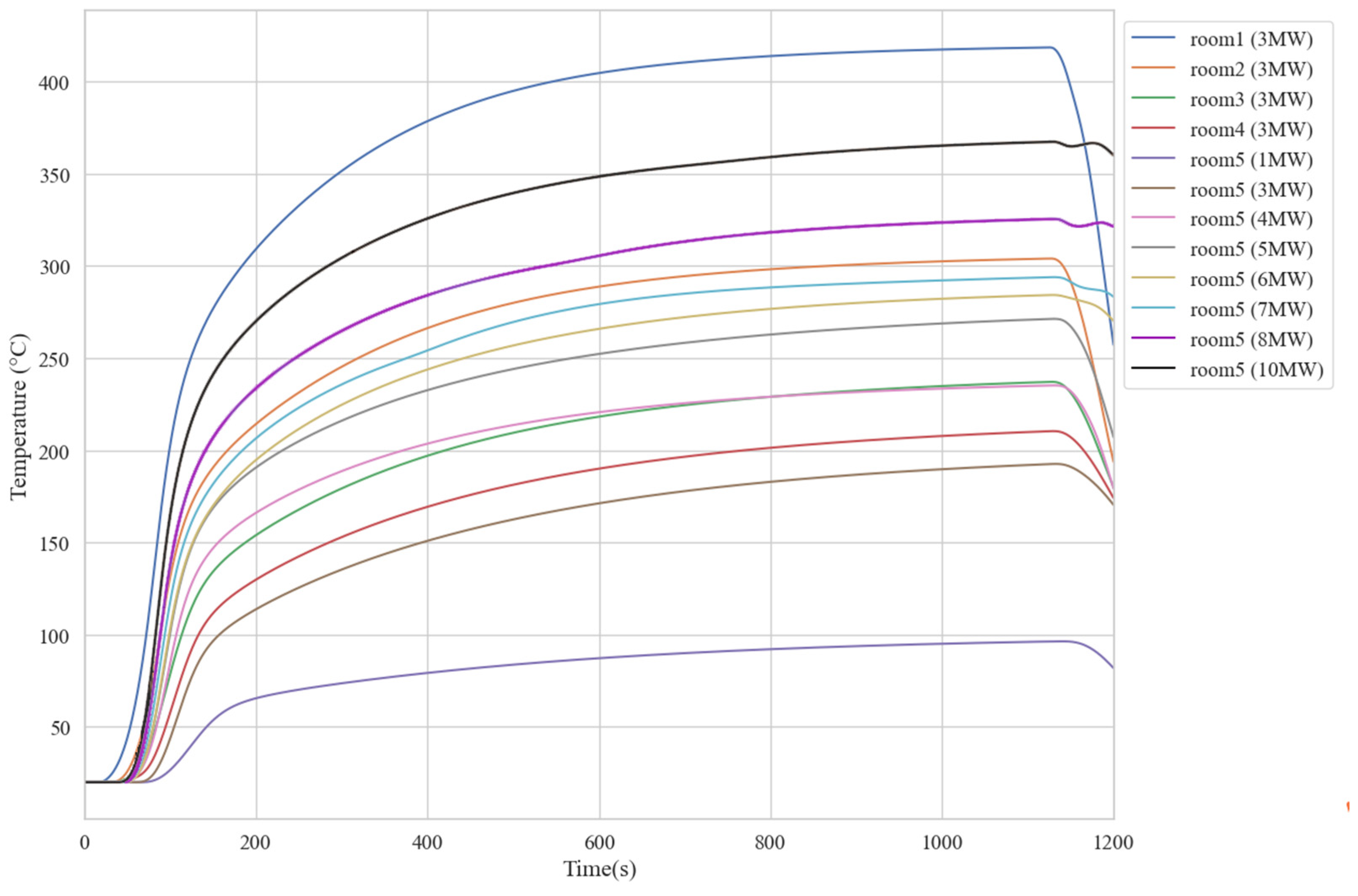
After the onset of a fire, a substantial amount of smoke is generated and accumulates at the ceiling. Initially, it does not spread to the corridors; hence, sensors placed there show no significant change in readings. As the smoke spreads from the fire-originating room to the corridor and gradually to the adjacent corridors, the smoke layer temperature in the corridor’s upper part progressively increases. Various factors, including the location and heat release rate of the fire source, the size and position of openings, and the layout of the space, influence the movement and distribution of the smoke. As illustrated in Figure 2, data curves from temperature sensor 1 were selected under simulations of 12 different fire source settings. This paper aimed to utilize artificial intelligence models to identify the relationship between temperature data or its processed feature parameters and the fire source, thereby facilitating the determination of the fire source. The specific process is depicted in Figure 3:

4. Machine Learning Model

4.1. Data Preprocessing

Data preprocessing is a pivotal step in artificial intelligence, directly impacting the model’s performance and accuracy. This study primarily employed preprocessing measures such as categorization, segmentation, normalization, and removal of irrelevant data.

4.1.1. Label Categorization

The processed sample data needs to be labeled to train machine learning models more effectively. The current dataset labels were set based on the different fire source positions and HRR in the CFAST simulation. The database established for this study involved categorizing and labeling different types of fire sources.

4.1.2. Segmentation Processing

Selecting a period as the input allows the model to capture and learn the dynamic changes and trends of data over time. This approach is beneficial for identifying the complex nonlinear relationships between temperature and fire source information. When a machine learning model can discriminate temperature curves throughout the fire process, it can obtain more accurate information about the fire source. Although, it will lose the ability to perform in real time. In this paper, the dataset was processed in segments with a selected time interval of 30 s. The obtained data were respectively 30–60 s, 60–90 s, …, 1170–1200 s. After segmenting, 39 samples were obtained for each fire scenario. This study simulated 4800 fire scenarios, resulting in 187,200 samples.

4.1.3. Data Standardization

Normalization of the acquired sample data by converting dimensional expressions into dimensionless expressions, solving the comparability problem of the data.

4.1.4. Deletion of Useless Data

Each CFAST simulation obtained a data curve of 1200 s. As the sensors had a specific activation time, the data obtained during this period did not contribute to the model training. To improve the accuracy and efficiency of the model, the useless data in the first 30 s were removed, and only the data from the 30 s to 1200 s were used.

4.2. Feature Extraction

Feature extraction is a crucial process for obtaining feature vectors of data information. This paper extracted nine manual features based on temperature time series $\{T_1,T_2,\cdots ,T_i,\cdots ,T_n\}$ to better describe the information on different fire sources and to achieve optimal classification performance. Each sample had nine temperature curves, resulting in 81 features generated for each sample.

①

Maximum ($T_{\max }$): the highest value in the selected temperature time series.

②

Mean ($\mu$): the arithmetic average of a selected temperature time series, which reflected the average level of a temperature segment.

③

Minimum ($T_{\min }$): the lowest value in the selected temperature time series.

④

Standard deviation ($\sigma$): the arithmetic square root of the arithmetic mean of the squared deviations from the mean of a selected temperature time series, reflecting the degree of temperature dispersion in a period. The formula for calculating standard deviation is as follows:

$$\sigma =\sqrt{\frac{{\displaystyle {\sum }_{i=1}^n{\left(T_i-\mu \right)}^2}}{n}}$$

(6)

⑤

Mean absolute deviation (MAD): the average of the absolute deviations of all individual observed values in the selected temperature time series from their arithmetic mean, which avoided the situation where errors in a temperature segment cancelled each other out. The calculation formula is as follows:

$$MAD=\frac{1}{n}{\displaystyle \sum _{i=1}^n\left|T_i-\mu \right|}$$

(7)

⑥

Interquartile range (IQR): the interquartile range (IQR), which was the difference between the upper quartile (Q₃, located at 75%) and the lower quartile (Q₁, located at 25%) of the selected temperature time series, reflected the dispersion of the middle half of the temperature. The formula for calculating IQR is as follows:

$$IQR=Q_3-Q_1$$

(8)

⑦

Coefficient of variation (c): the ratio of the standard deviation to its corresponding mean in the selected temperature time series, a normalized measure of the temperature dispersion. The calculation formula is as follows:

$$c=\frac{\sigma }{\mu }$$

(9)

⑧

Skewness (SK): the ratio of the difference between the mean ($\mu$) and median ($m_0$) of a selected temperature dataset to its standard deviation, reflecting the degree of skewness of the temperature. The calculation formula is as follows:

$$SK=\frac{\mu -m_0}{\sigma }$$

(10)

⑨

Kurtosis (${\gamma }_2$): the number that reflected the sharpness of the peak of the selected temperature time series at the mean value. The calculation formula is as follows, where ${\mu }_4$ represents the fourth central moment:

$${\gamma }_2=\frac{{\mu }_4}{{\sigma }^4}-3$$

(11)

4.3. Construction of Fire Source Determination Model

This study used 81 (9 × 9) extracted features from a 30 s temperature time series as the input for the fire source determination model, which outputted the fire source classification results. The obtained samples were randomly shuffled and divided into quantities of 70% for training and 30% for testing. Furthermore, five-fold cross-validation was employed during the training process. Decision tree, random forest, and LightGBM were selected in this study and were individually fine-tuned using random search random searchand Bayesian optimization [32]. Random parameter tuning involved selecting parameters randomly from a given range of hyperparameters, while Bayesian tuning was an optimization method based on Bayesian probability principles. The tuning results are shown in

Table 3. Decision Tree Parameter Tuning Results.

Parameter	Explanation	Tuning Range	Tuning Results
Max_depth	The maximum depth of the decision tree. Depth was the number of nodes along the longest path from the root to a leaf.	(1, 30)	20
Min_samples_split	The minimum number of samples a node must have before it can be split.	(2, 50)	15
Min_samples_leaf	The minimum number of samples a leaf node must have.	(1, 50)	5
Max_features	The maximum number of features to consider when looking for the best split.	[‘sqrt’, ‘log2’]	Log2

,

Table 4. Random Forest Parameter Tuning Results.

Parameter	Explanation	Tuning Range	Tuning Results
Nestimators	The number of trees in the random forest.	(50, 300)	238
Max_depth	The maximum depth of the trees.	[3, 5, 10, None]	None
Max_features	The maximum number of features considered when finding the best split.	(1, 15)	6
Min_samples_split	The minimum number of samples required to split a node.	(2, 15)	10
Min_samples_leaf	The minimum number of samples required to be at a leaf node.	(1, 11)	4
Bootstrap	Whether bootstrap sampling was used when building trees.	[True, False]	False
Class_weight	The weights used for classes in handling imbalanced datasets.	[‘balanced’, ‘balanced_subsample’, None]	balanced

and

Table 5. LightGBM Parameter Tuning Results.

Parameter	Explanation	Tuning Range	Tuning Results
Bagging_fraction	The proportion of sub-samples used in the bagging process.	(0.5, 1)	0.9511
Min_data_in_leaf	The minimum amount of data required in a leaf node.	(1, 100)	40
Max_depth	The maximum depth of the trees.	(3, 20)	16
Min_split_gain	The minimum gain required to perform a split.	(0, 5)	0.001
Num_leaves	The maximum number of leaf nodes in a tree.	(16, 128)	81
Lambda_l1	The weight of the L1 regularization term.	(0, 1)	0.3516
Lambda_l2	The weight of the L2 regularization term.	(0, 1)	0.4062

.

4.4. Evaluation Metrics

In this paper, precision (P), recall (R), and F₁-score (F₁) were used as evaluation metrics for the classification model. P_i represents the proportion of samples predicted as class i that were actually class i. In contrast, R_i represents the ratio of correctly predicted class i samples to actual class i samples. The F₁ score was the weighted harmonic mean of precision and recall. Specifically, the formulas for calculating the three metrics are as follows:

$$P_i=T{P}_i/(T{P}_i+F{P}_i)$$

(12)

$$R_i=T{P}_i/(T{P}_i+F{N}_i)$$

(13)

$$F_{1i}=2P{R}_i/(P_i+R_i)$$

(14)

In which, TP_i (true positive) represents the samples of class i that were correctly predicted as class i; FP_i (false positive) represents the samples of other classes that were predicted as class i; FN_i (false negative) represents the samples of class i that were predicted as other classes.

In this task, since it involves the classification of multiple categories, macro average metrics needed to be used to evaluate the classification model’s performance from an overall perspective. The specific calculation formula for the macro-average is shown below where k = 10 is the arithmetic average of accuracy and recall, and F₁ score of each category. Macro-average was commonly used to evaluate a classification model’s performance on multiple datasets.

$$P_{\mathrm{macro}} = \frac{1}{k}{\displaystyle \sum _{i=1}^k{P}_i}$$

(15)

$$R_{\mathrm{macro}}=\frac{1}{k}{\displaystyle \sum _{i=1}^k{R}_i}$$

(16)

$$F_{1\mathrm{macro}}=\frac{1}{k}{\displaystyle \sum _{i=1}^k{F}_{1i}}$$

(17)

4.5. Performance Evaluation of the Model

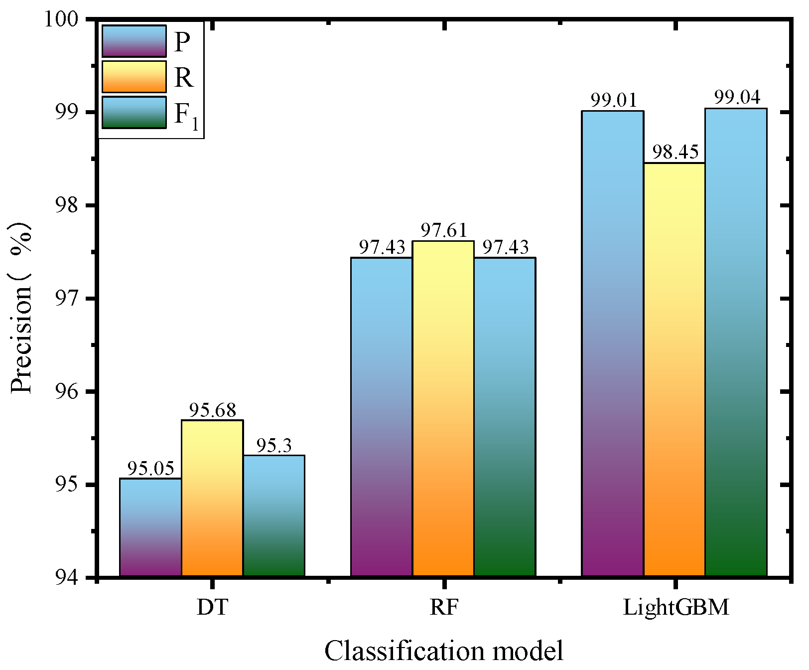
Based on the evaluation metrics, to verify the effectiveness of the three machine learning models established in the task of underground commercial street fire source determination, the experiment used the extracted features of the test set as model inputs and compared the classification performance of decision tree, random forest, and LightGBM models. The comparative experimental results are shown in Figure 4.

As can be seen from Figure 4, the LightGBM model achieved the best evaluation metrics, with macro averages of precision, recall, and F₁ score being 99.01%, 98.45%, and 99.04%, respectively. These metrics indicated that the LightGBM model accurately identifies and classified fire sources. A precision rate of 99.01% suggests that the model rarely made false positive predictions, while a recall rate of 98.45% indicated that nearly all actual fire sources were correctly identified, with minimal missed detections. An F₁ score of 99.04% emphasized the model’s excellent balance between precision and recall. These results demonstrated LightGBM’s formidable capability in handling challenging multi-classification tasks, primarily due to the training set’s complex nonlinear relationship between temperature data and fire source information. Compared to the RF and DT models, LightGBM’s histogram algorithm and controllable depth leaf-wise growth strategy significantly leveraged its advantages.

Furthermore, the RF model’s evaluation metrics were all higher than the DT model’s, with increases in macro averages of precision, recall, and F₁ score by 2.38%, 1.93%, and 2.13%, respectively. This improvement was attributed to the random forest’s ensemble method and its ability to handle high-dimensional data, resulting in a higher prediction accuracy than a single decision tree in complex multi-classification tasks like fire source classification.

In summary, the LightGBM, RF, and DT models exhibited unique strengths. LightGBM exceled in this task, owing to its outstanding class differentiation ability and high-dimensional data processing capability, enabling it to identify and classify complex data patterns effectively. As an ensemble method of decision trees, the random forest also demonstrated excellent performance, particularly in reducing overfitting and handling of high-dimensional data. In contrast, a single decision tree may be less effective in complex classification problems. Therefore, considering the characteristics of fire source classification, LightGBM, and RF models are more suitable for further research and improvement.

4.6. Kappa Coefficient

The kappa coefficient is a statistical method used to evaluate consistency and is commonly used to evaluate multi-class models accurately. The coefficient ranges [−1, 1] but is typically normalized to [0, 1] in practical applications. The higher the coefficient value, the higher the accuracy of the classification achieved by the model. The kappa coefficient is calculated using the following formula:

$$\mathit{k}=\frac{p_0-p_e}{1-p_e}$$

(18)

In which, $p_0$ represents the ratio of the sum of the correctly classified samples in each fire source category to the total number of samples. $p_e$ refers to the probability of the classifier agreeing with the actual labels by chance in a completely random scenario.

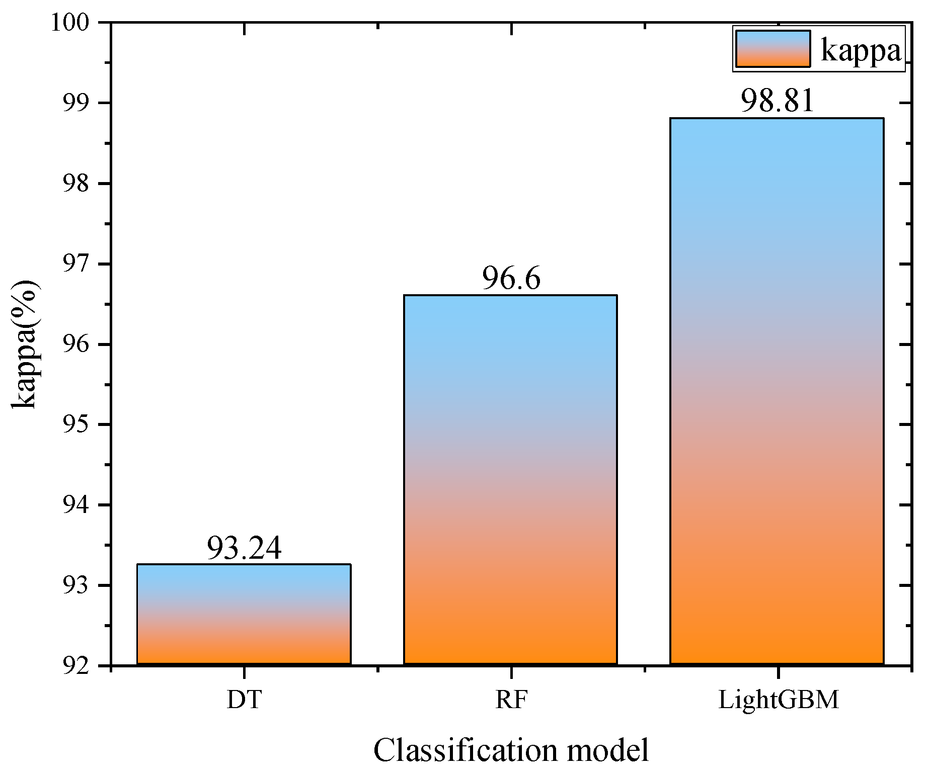
The kappa coefficients of the three models are illustrated in Figure 5. The figure shows that the LightGBM model exhibited the best performance with a kappa value of 98.81%, signifying near-perfect classification performance and demonstrating remarkable consistency. Meanwhile, although the kappa value of the RF model was slightly lower than that of LightGBM, it still surpassed the DT model. This advantage was attributed to its random feature selection and multi-tree voting mechanism, which maintained good accuracy.

4.7. Application of Fire Source Determination Technology in Real Fire Situations

Fire source identification is crucial to fire risk assessment and emergency response. In an underground commercial street, the application of artificial intelligence fire source determination technology for fire risk assessment and emergency response in real fire situations can proceed as follows.

(1)

Real-time fire source identification

① The artificial intelligence model analyses temperature sensor data from the corridors of the underground commercial street to locate fire source information accurately.

② The system automatically triggers a fire alarm and communicates the fire source information to the emergency response center and the building management system.

(2)

Fire emergency response

Based on fire source information, the emergency response center rapidly deploys firefighting, medical, and rescue teams, ensuring effective response tailored to the specific details of the fire source.

(3)

Evacuation plan optimization

① The building management system automatically adjusts evacuation instructions based on the specific location of the fire source, guiding personnel through electronic displays or broadcast systems within the commercial street to the safest evacuation routes.

② The monitoring center continuously tracks the evacuation of personnel, ensuring the safe withdrawal of all individuals.

(4)

Risk assessment and safety strategy

① After the event, using data provided by the artificial intelligence model and records of the fire situation, assess the fire risk of the underground commercial street.

② Based on the risk assessment results, adjust and optimize the underground commercial street’s fire prevention measures, safety system design, and emergency response plans.

(5)

Continuous monitoring and improvement

① In day-to-day operations, continuously monitor and analyze temperature sensor data to promptly identify potential risks and implement preventive measures.

② Regularly review and update the artificial intelligence model to ensure accuracy and adaptability, thereby better addressing potential fire incidents.

5. Conclusions

This paper established a fire source determination method for underground commercial streets based on temperature and machine learning. It constructed fire source determination models for underground commercial streets using three machine learning algorithms: RF, DT, and LightGBM. The paper calculated the macro averages of precision, recall, and F₁ scores for the three models and performed a comparative analysis of their kappa values, leading to the following conclusions:

(1)

The LightGBM model performed best in determination with its exceptional class differentiation ability and high-dimensional data processing capability. Its macro averages for precision, recall, and F₁ score were 99.01%, 98.45%, and 99.04%, and its kappa value was 98.81%.

(2)

The high determination performance of the three machine learning models indicated that the fire database established through CFAST simulation, based on random sampling for determining fire conditions, was more aligned with the objective laws of the real world.

(3)

This study’s three machine learning models demonstrated strong classification capabilities and interpretability.

The fire source determination method proposed in this study offers technical support for the management of fire situations in underground commercial streets. In subsequent research, consideration should be given to how artificial intelligence technology can be better applied in fire risk assessment and emergency response. Furthermore, the variety of fire sources and the development of fires in real scenarios are more complex. To enhance the precision and practical value of fire source determination in underground commercial streets, future research should focus on two aspects: firstly, increasing sample data to enable the model to understand new categories better and to capture fire source characteristics, thereby improving determination accuracy; secondly, improving training models, such as adopting more advanced machine learning algorithms, to enhance the model’s generalizability and practical application value.

References

1. Chinese, A.; Chinese, S. 2021 Blue Book of China’s Urban Underground Space Development; China Science Publishing &Media LTD. (CSPM): Beijing, China, 2021; pp. 5–6. [Google Scholar]
2. Zhang, X.; Wan, J. Study on fire risk factors of underground commercial street based on DEMATEL/ISM. Ind. Saf. Environ. Prot. 2022, 48, 46–49. [Google Scholar]
3. Song, B.; Li, J. The key elements of decision making and its application on first due commander in fire fighting. Fire Sci. Technol. 2008, 27, 277–280. [Google Scholar]
4. Wu, Z.; Dang, W.; Yu, A.; Bai, Y. Discussion on quantitative risk assessment procedure in petrochemical enterprises. Saf. Health Environ. 2010, 10, 35–38. [Google Scholar]
5. Shu, S.; Zhang, Y.; Lu, Z.; Wang, D.; Jiang, N. Real-time prediction of heat release rate based on machine learning. Fire Saf. Sci. 2022, 31, 8–14. [Google Scholar]
6. Deng, L.; Tang, F.; Hu, P. Physical modeling and machine learning of ceiling maximum temperature rise induced by tandem heat sources with unequal heat release rates in a natural ventilation tunnel. Int. J. Heat Mass Transf. 2022, 197, 123333. [Google Scholar] [CrossRef]
7. Saeed, F.; Paul, A.; Hong, W.; Seo, H. Machine learning based approach for multimedia surveillance during fire emergencies. Multimed. Tools Appl. 2020, 79, 16201–16217. [Google Scholar] [CrossRef]
8. Liu, Q.; Zhu, B.; Deng, L.; Shi, H.; Liang, G. Double parameters fire detection method based on machine learning. China Saf. Sci. J. 2022, 32, 90–96. [Google Scholar]
9. Hodges, J.; Lattimer, B.; Luxbacher, K. Compartment fire predictions using transpose convolutional neural networks. Fire Saf. J. 2019, 108, 102854. [Google Scholar] [CrossRef]
10. Yan, D.; Feng, X. Research on Fire Source Localization Method Based on Wireless Sensor Networks. Technol. Innov. Appl. 2016, 25, 106–107. [Google Scholar]
11. Sun, M. Performance Improvement for Distributed Fiber Temperature Sensor System and Research on Fire Source Localization. Ph.D. Thesis, University of Science and Technology of China, Hefei, China, 2017. [Google Scholar]
12. Chu, H.; Zhao, Y.; Zhuang, B.; Wang, Y.; Yang, X. Fire location and detection system based on computer vision technology. Electron. Des. Eng. 2020, 28, 156–160+164. [Google Scholar]
13. Shen, D. Application Research of Bayesian Machine Learning in Fire Forecasting and Source Intensity Back-Calculation. Master’s Dissertation, University of Science and Technology of China, Hefei, China, 2021. [Google Scholar]
14. Wu, X.; Zhang, X.; Huang, X.; Xiao, F.; Usmani, A. A real-time forecast of tunnel fire based on numerical database and artificial intelligence. Build. Simul. 2022, 15, 511–524. [Google Scholar] [CrossRef]
15. Zhang, X.; Wu, X.; Park, Y.; Zhang, T.; Huang, X.; Xiao, F.; Usmani, A. Perspectives of big experimental database and artificial intelligence in tunnel fire research. Tunn. Undergr. Space Technol. 2021, 108, 103691. [Google Scholar] [CrossRef]
16. Wu, X.; Park, Y.; Li, A.; Huang, X.; Xiao, F.; Usimani, A. Smart detection of fire source in tunnel based on the numerical database and artificial intelligence. Fire Technol. 2021, 57, 657–682. [Google Scholar] [CrossRef]
17. Breiman, L. Classification and regression trees. Rev. Des Mal. Respir. 2004, 21, 1174–1176. [Google Scholar]
18. Chen, Y.; Wu, J.; Xu, K. Using Gini-index-for attribute selection in decision trees. Microcomput. Dev. 2004, 66–68. [Google Scholar]
19. Breiman, L. Random forests. Mach. Learn. 2001, 45, 5–32. [Google Scholar] [CrossRef]
20. Cao, Y.; Miao, Q.; Liu, J.; Gao, L. Advance and prospects of Adaboost algorithm. Acta Autom. Sin. 2013, 39, 745–758. [Google Scholar] [CrossRef]
21. Ke, G.; Meng, Q.; Finley, T.; Wang, T.; Chen, W.; Ma, W.; Ye, Q.; Liu, T. LightGBM: A highly efficient gradient boosting decision tree. In Proceedings of the 31st Annual Conference on Neural Information Processing Systems (NIPS), Long Beach, CA, USA, 4–9 September 2017; pp. 3149–3157. [Google Scholar]
22. Peacock, R.; Mcgrattan, K.; Forney, G.; Reneke, P. Cfast—Consolidated Fire and Smoke Transport (Version 7) Volume 1: Technical Reference Guide; National Institute of Standards and Technology: Gathersburg, MD, USA, 2021. [Google Scholar]
23. Chow, W. Multi-cell concept for simulating fires in big enclosures using a zone model. J. Fire Sci. 1996, 14, 186–198. [Google Scholar] [CrossRef]
24. Reneke, P.; Peacock, R.; Gilbert, S.; Cleary, T. Cfast—Consolidated Fire and Smoke Transport (Version 7) Volume 5: Cfast Fire Data Generator (Cdata); National Institute of Standards and Technology: Gathersburg, MD, USA, 2021. [Google Scholar]
25. Peacock, R.; Forney, G.; Reneke, P. Cfast—Consolidated Fire and Smoke Transport (version 7) Volume 3: Verification and Validation Guide. National Institute of Standards and Technology: Gathersburg, MD, USA, 2021. [Google Scholar]
26. Bailey, J.; Forney, G.; Taterm, P.; Jones, W. Development and validation of corridor flow submodel for CFAST. J. Fire Prot. Eng. 2002, 12, 139–161. [Google Scholar] [CrossRef]
27. Jones, W.; Forney, G. Improvement in predicting smoke movement in compartmented structures. Fire Saf. J. 1993, 21, 269–297. [Google Scholar] [CrossRef]
28. Fan, N. Research on Method of Fire Simulation in Long-Narrow Confined Space Based on Cfast. Master’s Thesis, AnHui University of Science and Technology, Huainan, China, 2009. [Google Scholar]
29. Chow, W. Simulation of tunnel fires using a zone model. Tunn. Undergr. Space Technol. 1996, 11, 221–236. [Google Scholar] [CrossRef]
30. Bruns, M. Estimating the Flashover Probability of Residential Fires Using Monte Carlo Simulations of the MQH Correlation. Fire Technol. 2018, 54, 187–210. [Google Scholar] [CrossRef]
31. GB 51251-2017; Technical Standard for Smoke Management Systems in Buildings. China Planning Press: Beijing, China, 2017.
32. Zhang, A.; Yang, Z. Hyperparameter tuning methods in automated machine learning. Sci. Sin. Math. 2020, 50, 695–710. [Google Scholar]
Figure 1. CFAST model diagram of underground commercial street.
Fire 07 00053 g001
Figure 2. Temperature curve for corridor 1.
Fire 07 00053 g002
Figure 3. The work-flow of the proposed model.
Fire 07 00053 g003
Figure 4. Comparison chart of classification results.
Fire 07 00053 g004
Figure 5. Kappa coefficients of the three algorithms.
Fire 07 00053 g005