Article

Attention-Based Wildland Fire Spread Modeling Using Fire-Tracking Satellite Observations

1
Our Kettle Inc., Kensington, CA 94707, USA
2
Department of Earth System Science, University of California, Irvine, CA 92697, USA
3
School of Earth and Environmental Sciences, Cardiff University, Cardiff CF10 3AT, UK
4
Department of Earth and Environmental Engineering, Columbia University, New York, NY 10027, USA
*
Author to whom correspondence should be addressed.
Fire 2023, 6(8), 289; https://doi.org/10.3390/fire6080289
Submission received: 28 June 2023 / Revised: 25 July 2023 / Accepted: 26 July 2023 / Published: 29 July 2023

Abstract

:
Modeling the spread of wildland fires is essential for assessing and managing fire risks. However, this task remains challenging due to the partially stochastic nature of fire behavior and the limited availability of observational data with high spatial and temporal resolutions. Herein, we propose an attention-based deep learning modeling approach that can be used to learn the complex behaviors of wildfires across different fire-prone regions. We integrate optimized spatial and channel attention modules with a convolutional neural network (CNN) modeling architecture and train the attention-based fire spread models using a recently derived fire-tracking satellite observational dataset in conjunction with corresponding fuel, terrain, and weather conditions. The evaluation results and their comparison with benchmark models, such as a deeper and more complex autoencoder model and the semi-empirical FARSITE fire behavior model, demonstrate the effectiveness of the attention-based models. These new data-driven fire spread models exhibit promising modeling performances in both the next-step prediction (i.e., predicting fire progression from one timestep earlier) and recursive prediction (i.e., recursively predicting final fire perimeters from initial ignition points) of observed large wildfires in California, and they provide a foundation for further practical applications including short-term active fire spread prediction and long-term fire risk assessment.

1. Introduction

The western US is facing intensified fire risks stemming from increasing large wildfire hazards [1,2] and escalating exposure levels [3] across the region. The observed increase in the occurrence of hazardous wildfires and the associated socioeconomic burden on infrastructure and livelihoods [4] have been attributed to a range of drivers, including worsening fire-prone weather conditions [5] due to global climate change [6,7,8], increasing contributions from human ignitions [9], the rapid expansion of the wildland–urban interface (WUI) [10], and the failure of the longstanding wildfire suppression policy, causing the accumulation of flammable fuel [11]. As society mitigates and adapts to these new threatening conditions [12], it is necessary to understand the spatial and temporal changes in evolving wildfire risks across the region. Both the public and private sectors are increasing their investments in the above wildfire-related research fields to address the growing threat of wildfire risks.
To meet the needs of fire risk assessment and prediction over daily to decadal timescales, various modeling tools have been developed to simulate essential burning processes, encompassing fire ignition, spread, and associated impacts. These models utilize different approaches, including physics-based models, data-driven models, or a combination of both, to capture the complexities of fire behavior and its spatiotemporal dynamics. Physics-based fire models, as outlined in the referenced review paper [13], are based on mathematical equations that describe fundamental combustion processes, including thermal radiation and fluid dynamics. Developing and implementing these models typically require significant computational resources due to their reliance on complex simulations. On the other hand, data-driven models take an empirical approach to directly learn the intricate relationships and patterns of fire behavior from observed data [14]. This allows data-driven models to capture the complexities of fire dynamics without relying on explicit equations. The data-driven models can be further categorized into statistical models, machine learning models, and deep learning models based on the complexity and characteristics of the modeling techniques employed. Some widely used fire spread models include semi-empirical community-scale models like FARSITE [15] and FlamMap [16], a global-scale CESM fire model [17], level-set models such as ELMFIRE [18] and WRF-SFIRE [19], Celluar Automata models [20], and recently developed machine learning (ML)-/deep learning (DL)-based models [21,22,23,24].
The rapid advances of ML-/DL-based fire spread models show intriguing advantages in computational efficiency and flexibility, although their modeling capabilities for practical applications still need to be improved. Both the limited availability of observational fire data at high spatiotemporal resolutions and the lack of optimized modeling architectures designed for learning complex fire behavior tend to hinder the further improvement of data-driven fire spread models. To address these problems, we develop new modeling architectures inspired by physical fire spread processes to learn how fire propagates in wildlands, as observed in a recently derived fire-tracking satellite observation dataset recorded by the Visible Infrared Imaging Radiometer Suite (VIIRS) instrument [25]. This novel object-based Fire Event Data Suite (FEDS), with continuous tracking of fire progression throughout its lifetime, provides unprecedented opportunities to train new data-driven fire spread models at a high spatiotemporal resolution. We tackle the fire spread modeling problem via the following two steps: (1) next-step prediction that predicts fire progression in subsequent timesteps based on model inputs from one step earlier (i.e., X f i r e t Y ^ f i r e t + 1 ) and (2) recursive prediction that predicts final fire perimeters from initial ignition points, using next-step prediction recursively (i.e., X f i r e t 0 Y ^ f i r e t 1 Y ^ f i r e t n ). The majority of the previous ML-/DL-based fire modeling studies primarily focused on addressing the first problem, while comparatively less attention have been provided to the second problem. While recursive prediction poses greater challenges due to the accumulation and amplification of modeling errors throughout the iterative process, it holds greater practical value for simulating the complete lifecycles of fire events and assessing their comprehensive physical and socioeconomic impacts. For instance, the capability to model complete fire events is crucial for conducting tail risk assessment within the insurance industry. This is because most fire losses are caused by catastrophic large wildfires, and historical data pertaining to such extreme events are often limited in their availability. Furthermore, the evolving fire weather conditions associated with climate change render fire risk factors non-stationary, rendering historical loss records insufficient for accurate fire risk assessment. Therefore, it is imperative to develop improved fire models that incorporate climate change factors, enabling the simulation of growing extreme fire events for proactive risk assessment.
In this study, three convolutional neural network (CNN) models integrated with different fire attention mechanisms were developed to achieve the above goal. We trained and evaluated these CNN fire models using the novel FEDS fire-tracking observational dataset from 2012–2020 [25]. The training datasets and modeling architectures are described in Section 2, with more details provided in Appendix A. Section 3 presents the model evaluation results and their comparison with benchmark models, followed by more discussion in Section 4 and conclusional remarks in Section 5.

2. Materials and Methods

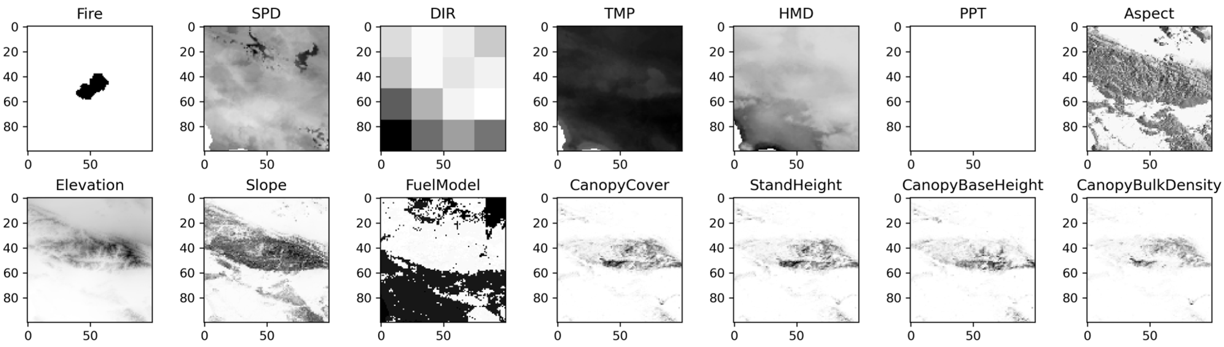
2.1. Observation-Based Model Inputs

We used model input settings in our CNN fire spread models that were similar to the model input setting of the semi-empirical FARSITE fire behavior model [15], including 14 input features in 4 groups for fire, terrain, fuel, and weather conditions. The predictands were fire polygons at the next timesteps (next-step prediction) or final timesteps (recursive prediction). The model input data were collected from multiple sources, as listed below:
Observational fire data: The daily progression of 735 large wildfires (fire size ≥ 4 km2) during the period 2012–2020 in California were derived from VIIRS satellite observations at a spatial resolution of ~375 m and a 12 h temporal resolution [25]. This object-based FEDS dataset contains the direct serialization of all fire objects, core fire properties, and vector geometries at each timestep, and it was used as one of model inputs to predict fire polygons in next-step prediction as well as a ground truth to evaluate the predicted results.
Terrain data: Three topographic variables (i.e., Aspect, Elevation, and Slope) at a 30 m spatial resolution were collected from the LANDFIRE program [26].
Fuel data: Five fuel variables (i.e., FuelModel, CanopyCover, StandHeight, CanopyBulkDensity, and CanopyBaseHeight) at a 30 m spatial resolution were also collected from the LANDFIRE program [27]. Among these fuel variables, FuelModel is short for the 13 Anderson Fire Behavior Fuel Models (FBFM13), which represent distinct distributions of fuel loading among surface fuel components, size classes, and fuel types. The other four variables represent forest canopy characteristics such as canopy cover, canopy height, canopy bulk density, and canopy base height, respectively. The LANDFIRE fuel products were updated on a roughly biennial basis. We used the most recent fuel products before each observed fire event to capture vegetation dynamics and prior fuel disturbances in the model.
Weather data: Four daily weather variables (i.e., TMP: maximum air temperature; HMD: relative humidity; PPT: precipitation; and SPD: wind speed) at a 1 km spatial resolution were developed through the NEX-GDM program [28] and collected from the NASA GeoNEX data portal [29]. Note that these NEXGDM weather data do not provide wind direction. We collected 10 m u-/v-components of wind from the ERA5 hourly reanalysis product [30] at a spatial resolution of 0.25° from the Copernicus Climate Change Service website and then derived the surface wind direction (DIR: wind direction) as a complement.
After data collection, we pre-processed all the input data and resampled them to the same 1 km resolution on a daily basis. For example, the data at higher raw spatial resolutions (e.g., the terrain and fuel variables) were aggregated from 30 m to 1 km using a spatial mean for continuous variables or a spatial mode for categorical variables, while other data at lower raw spatial resolutions (e.g., u-/v-components of wind) were interpolated to the same 1 km resolution using the bi-linear interpolation method. The vectorized FEDS fire-tracking data were rasterized as binary raster images, with 1 for burned pixels and 0 for non-burned pixels. Other input data were scaled from 0 to 1 before feeding them into the models. We then extracted and cropped these pre-processed data to images measuring 100 × 100 pixels (i.e., 100 km × 100 km tiles) with centers located around the ignition points of corresponding fires. The static inputs (i.e., terrain and fuel) were concatenated to the dynamically varying inputs (i.e., fire and weather) at each timestep. Figure 1 shows an example of processed model inputs at one timestep.

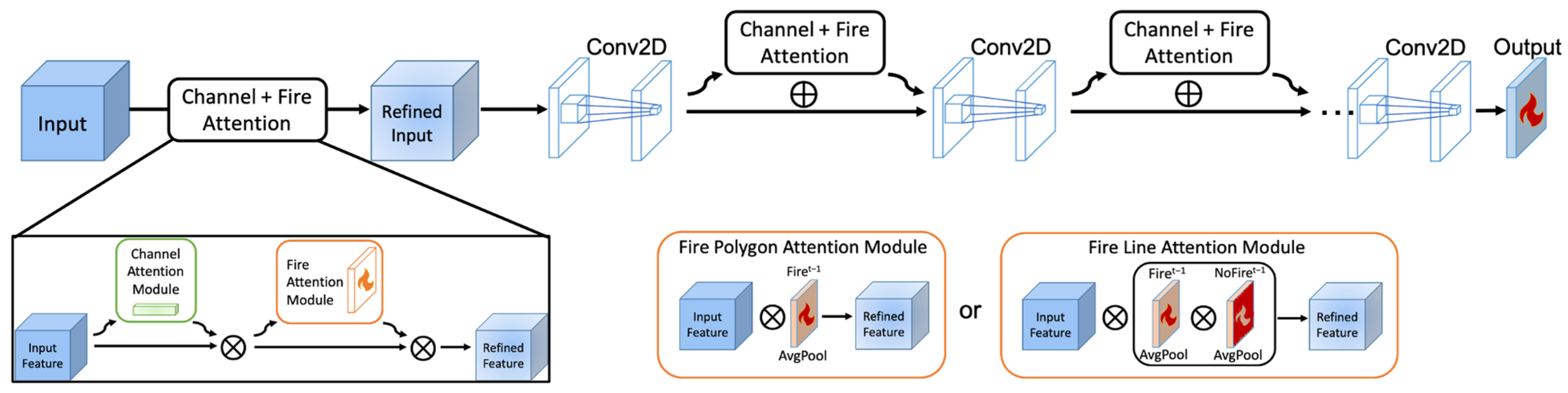
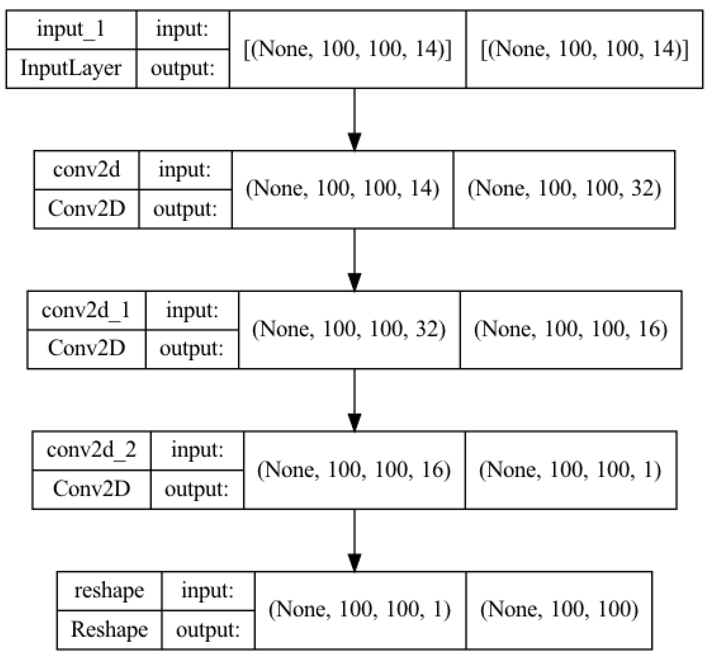
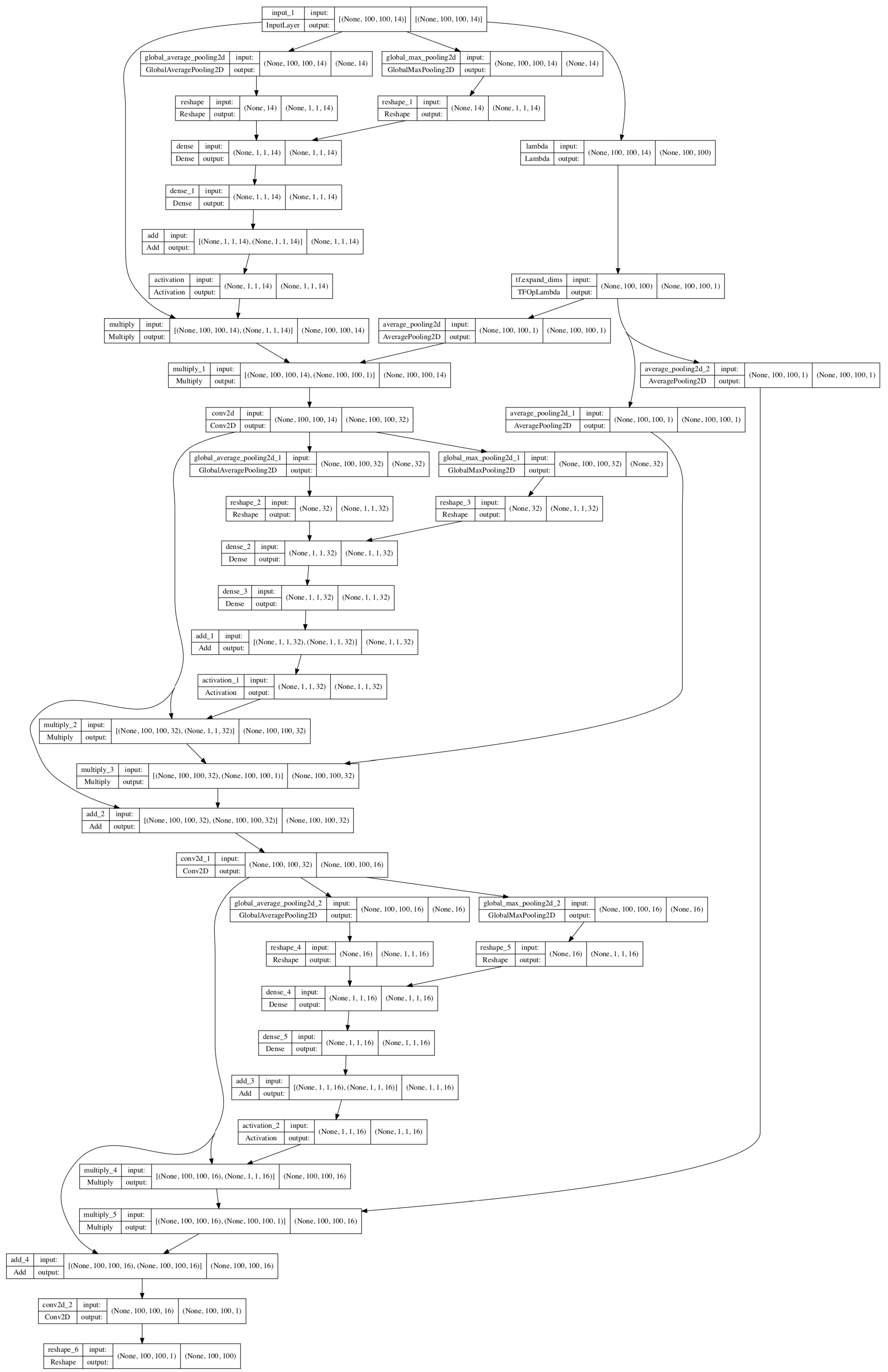
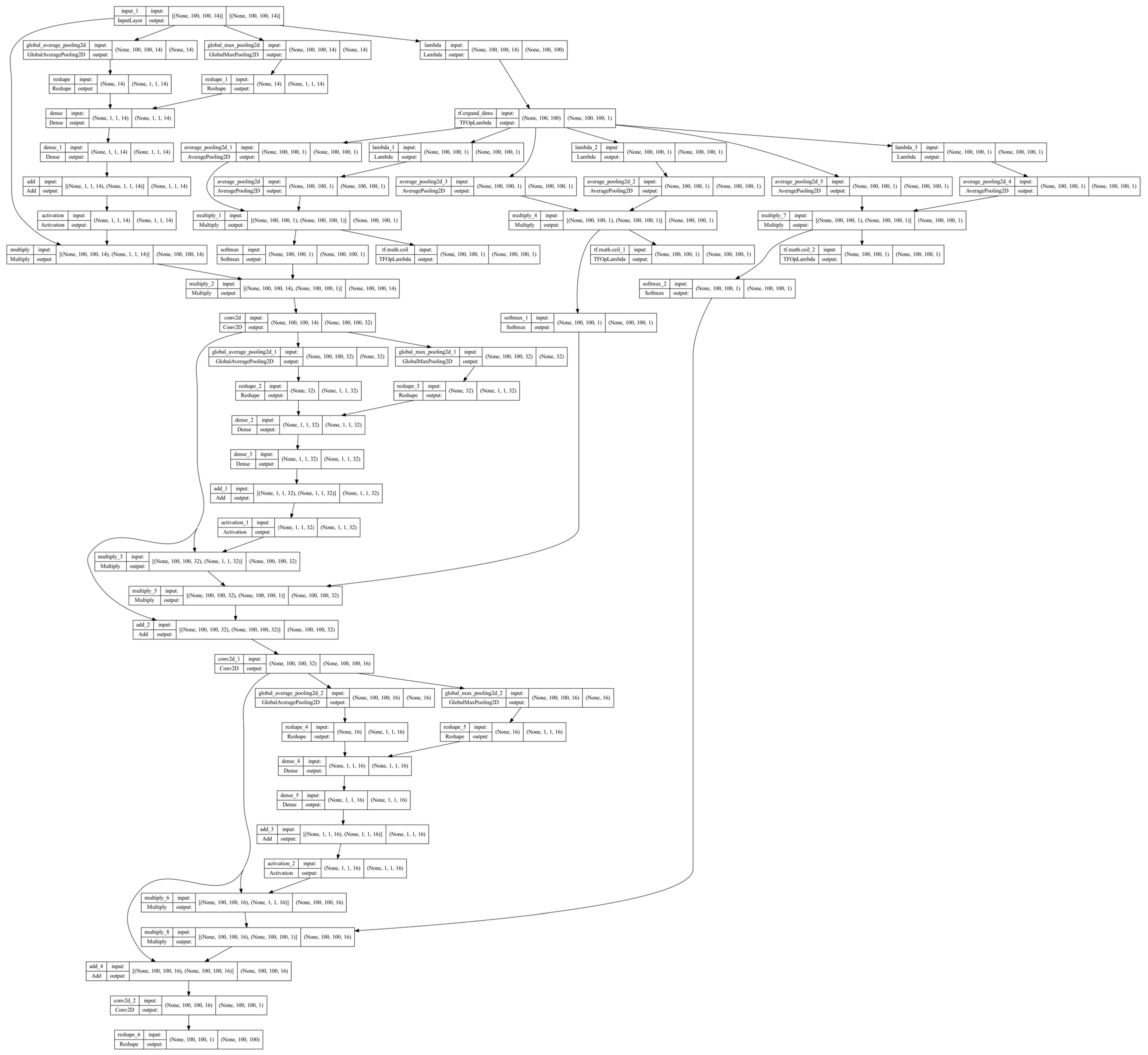
2.2. Model Architectures

We developed three fire spread models by integrating different fire attention modules with a multi-layer CNN architecture via skip connections (Figure 2). The fire and channel attention modules were adopted and improved from a “Convolutional Block Attention Module” (CBAM) [31] to enhance the feature representation in the CNNs at both the spatial and channel levels. The fire attention modules apply spatial attention to different fire areas to adjust 2D weights in the input feature maps in a spatially heterogeneous way during model training and inferencing. The following two fire attention modules are available as options: a module that concentrates on entire fire polygons from previous timesteps (FirePolyAttn: Fire Polygon Attention Module) and another module that specifically focuses on fire frontlines along the edges of fire polygons at previous timesteps (FireLineAttn: Fire Line Attention Module). These two fire attention modules draw inspiration from physical fire spread processes and are implemented by utilizing average pooling across different areas of input fire polygons from previous timesteps. Specifically, the fire polygon attention module employs average pooling over entire fire polygons, assigning higher weights to interior areas and lower weights to the edges of the fire polygons (Figure 3a). Conversely, the fire line attention module performs average pooling over both fire polygons and the residual areas outside of the fire polygons, respectively, followed by the multiplication of the pooling results to accentuate the edge areas of each fire polygon (Figure 3b). The channel attention module is the same as the original one in CBAM, which adjusts weights for different input features in a spatially homogeneous way. It uses the global average and max pooling to capture the most salient features in each channel and then uses the resulting 1D attention weights to focus on important channels. By implementing different attention modules in a basic CNN architecture, we developed three different fire spread models: CNN_NonAttn, without any attention module, CNN_FirePolyAttn, with the channel and fire polygon attention modules, and CNN_FireLineAttn, with the channel and fire line attention modules. Figure A1, Figure A2 and Figure A3 show their architecture graphs, followed by more details about the calculation of attention weights in Appendix A.
All the three CNN models employ a 3 × 3 kernel size and utilize “same” padding to maintain consistent spatial dimensions between the inputs and outputs of each layer. A rectified linear activation (ReLU) function is applied to the hidden layers, while a sigmoid function is used for the output layers. It is worth noting that these CNN models, with or without distinct fire attention modules, predict fire spread in different ways. For instance, CNN_NonAttn and CNN_FirePolyAttn directly predict the entire fire polygon for next timesteps ( Y ^ f i r e t + 1 ) based on model inputs at previous timesteps ( X f i r e t ) (Figure 3a), while CNN_FireLineAttn first predicts incremental changes in burned pixels between two consecutive timesteps ( Y ^ f i r e ) and then derives fire polygons at the next timesteps by adding the predicted changes in burned pixels to the fire polygon inputs from previous timesteps ( Y ^ f i r e t + 1 = X f i r e t + Y ^ f i r e ) (Figure 3b). The distinction in model prediction approaches significantly impacts the learning capabilities of these models, as evidenced by the evaluation results presented below.

2.3. Model Training, Validation, and Testing Methods

As previously mentioned, we adopted distinct prediction strategies for model training, validation, and testing. Next-step prediction was used for model training and validation, while recursive prediction was used for model testing. For model training and validation in next-step prediction, we used pairs of input data for 623 large wildfires which occurred during the 2012–2019 period in the FEDS data. Each pair represents data from two consecutive days coincident with fire observations. The data from the first day in the pair are considered dynamical model inputs X d y n _ v a r t (dyn_var indicates fire or weather variables) that exhibit spatiotemporal variations during fire simulations. These dynamical inputs were then concatenated with the static model inputs X s t a _ v a r (sta_var indicates terrain or fuel variables), which remain constant during fire simulations, resulting in complete model inputs comprising all 14 input features (Figure 1).
In next-step prediction, the observed fire polygons at the second timestep ( Y f i r e t + 1 ) in the pair serve as the ground truth for validating the model outputs ( Y ^ f i r e t + 1 ). The total 4788 pairs of consecutive frames from the 623 fires occurring in 2012–2019 were shuffled and split at a 9:1 ratio for model training and validation, respectively. To explore the influence of the training sample size on model performance, we employed a data augmentation technique by rotating all the input data by 90 degrees for three repetitions. The rotated data were then concatenated with the original non-rotated data to generate additional training samples. Once the model training and validation were completed, we used the first ( X f i r e t 0 ) and final frames ( Y f i r e t n ) of 103 large wildfires that lasted for at least two days in 2020 to test the well-trained model in the recursive prediction of continuous fire progression processes. It is worth noting that the chronological order of the model training and testing datasets is important for fire spread models because of the memory effect resulting from the impacts of previous fires on fuel input data such as reduced fuel loading and changes in fuel types after burning. This memory effect in fuel data, as one of the model inputs, can persist for several years and continuously influence future fire behavior in the years following historical fires. Regular updates to fuel data would aid the model in capturing and adapting to this memory effect in its fuel inputs.
Among all the model inputs, the fire feature is unique since its data sources are different between next-step prediction and recursive prediction. In next-step prediction, all fire inputs ( X f i r e t ) were from the VIIRS-derived satellite observations, which are one day earlier than the model outputs ( Y ^ f i r e t + 1 ). In recursive prediction, we only used VIIRS-derived fire ignition points at the very first timestep ( X f i r e t 0 ) as initial model inputs to predict model outputs at the second timestep ( X f i r e t 0 Y ^ f i r e t 1 ). We then repeated this next-step prediction process recursively by using model outputs from previous timesteps as new model inputs to sequentially predict fire in next days until the last day of each fire, as observed in the FEDS fire-tracking data ( Y ^ f i r e t 1 Y ^ f i r e t 2 Y ^ f i r e t n ).
For a model comparison, we used a simple persistent model assuming static fire shapes between two consecutive timesteps ( Y ^ f i r e t + 1 = X f i r e t ), the semi-empirical FARSITE fire behavior model [15], and a convolutional autoencoder model from Huot et al., 2021 [24] as the benchmarks. The autoencoder model showed the best performance in comparison with an additional three architectures presented in Huot et al., 2021 [24]. The model inputs for the autoencoder model are identical to the CNN models, with the only difference being that their spatial dimensions are cropped to images measuring 96 × 96 pixels to suit the autoencoder model’s requirements. The FARSITE model also uses the LANDFIRE fuel and terrain data, but at a considerably higher original resolution of 30 m. As for the weather inputs used in the FARSITE simulations, they were obtained from the ground weather stations nearest to the selected two fires. More detailed model information and the simulation settings of the autoencoder and FARSITE models are provided in Appendix A.
All the model simulations were evaluated using four metrics: recall, precision, F-1, and a precision–recall area under the curve (PR_AUC) score [32] if applicable. Here, the recall score represents the misdetection rate of the model (i.e., a higher recall value indicates a lower misdetection rate with fewer false negatives), the precision score represents the false alarm rate (i.e., a higher precision value indicates a lower false alarm rate with fewer false positives), and F-1 and PR_AUC represent combinations of the above two scores. The equations of evaluation metrics are provided below.
R e c a l l = T P T P + F N
P r e c i s i o n = T P T P + F P
F - 1 = 2 × R e c a l l × P r e c i s i o n R e c a l l + P r e c i s i o n = T P T P + 1 2 × F P + F N ,
here, TP stands for true positives, FN stands for false negatives, and FP stands for false positives. All these variables are calculated at the pixel level, with a true positive defined as an actually burned pixel that was correctly predicted to be positive, a false negative defined as an actually burned pixel that was incorrectly predicted to be negative, and a false positive defined as an actually non-burned pixel that was erroneously predicted to be positive. Table A1 shows the corresponding confusion matrix for this binary classification problem of fire spread prediction. In Table 1, all the metric scores were calculated by comparing the predicted fires ( Y ^ f i r e t n ) with the observed fires ( Y f i r e t n ) at the final timesteps of each fire and then averaging the value over the 103 large wildfires in 2020. Similarly, Table A2 lists the metric scores which were first calculated at each timestep of all wildfires in 2020 and then averaged over all the timesteps of their lengths of duration.
Since the binary fire data are highly imbalanced over the cropped 100 × 100 tiles, especially during the early stages of fire propagation after ignition (e.g., 1 ignited pixel vs. 9999 unburned pixels at fire ignition), we used a focal Tversky loss (FTL) function [33] to address this issue when training the models. This FTL function is a generalization of the Tversky loss based on the Tversky index (TI). By tuning hyperparameters such as α , β , and γ in the function, we can adjust the sensitivity of the model to different misclassification errors such as false negatives (FN) and false positives (FP).
F T L = 1 T I γ ,
T I = T P T P + α × F N + β × F P   , w h e r e   α + β = 1 .
Considering that the misdetection of active fires would cause more serious damage than a false alarm in practice, we set a larger α than β in the TI during model training to give a higher weight to recall than precision in our models. For simplicity, we used the same hyperparameter setting ( α = 0.75, β = 0.25, γ = 1.0) in the FTL for all the models trained in this paper.

3. Results

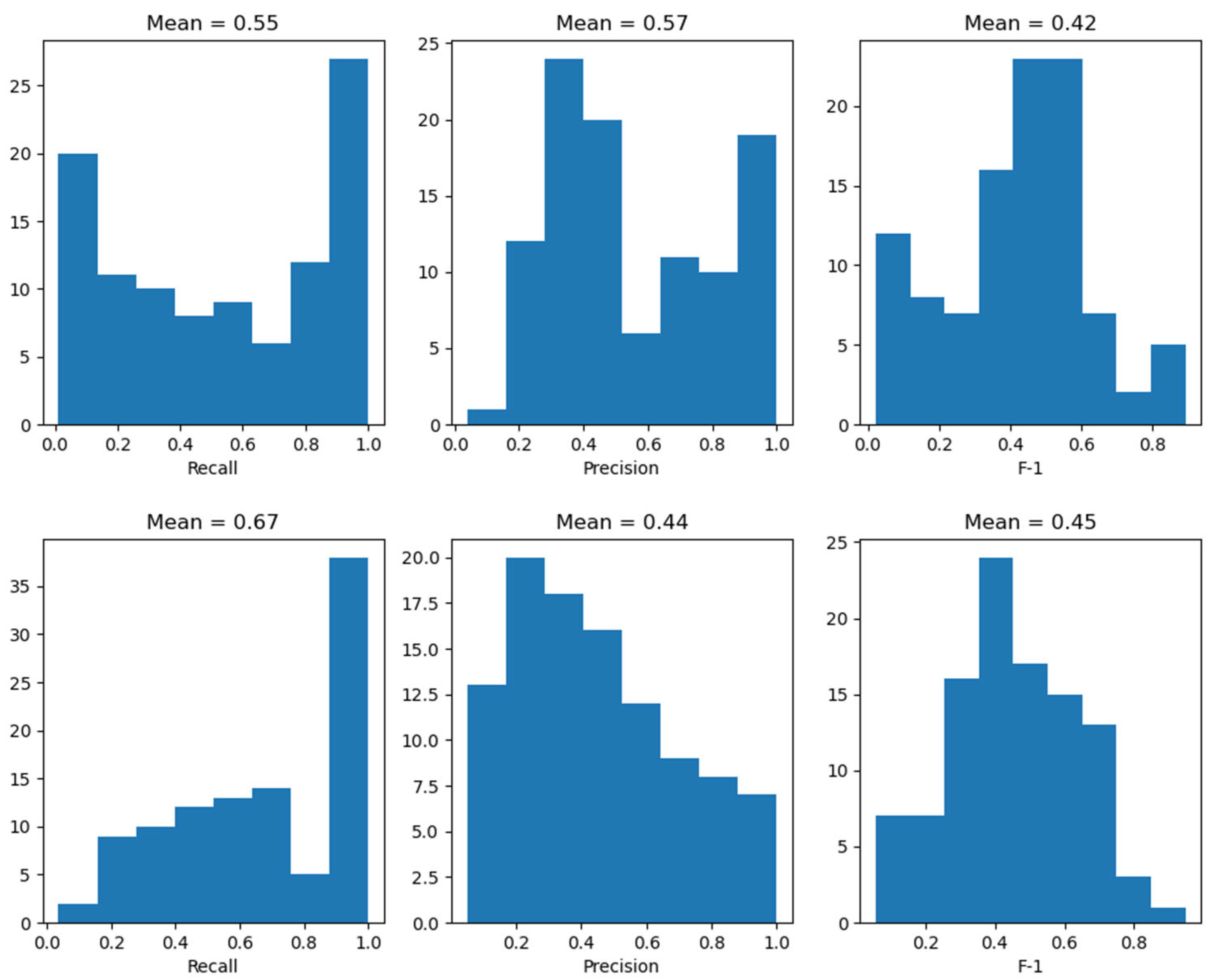
3.1. Metric Scores of Fire Spread Models

The distinction between model prediction approaches, as mentioned earlier, has a substantial impact on the learning proficiency of each model, particularly given the non-shrinking characteristics of fire. This is because an area burned by fire can only either monotonically increase or remain the same from one step to the next. Given the relatively short time interval of a single day in next-step prediction, it is very likely that fire polygons change marginally over two consecutive days ( Y f i r e = Y f i r e t + 1 X f i r e t 0 ) or even remain the same ( Y f i r e t + 1 = X f i r e t ) due to slow spread rates or human suppression. In this case, a persistent model with no predictability at all performs well given its static assumption ( Y ^ f i r e t + 1 = X f i r e t ). However, the persistent model fails completely in recursive prediction due to the accumulation of modeling errors throughout fire progression. This limitation is clearly demonstrated by the large differences in the recall and F-1 scores of the persistent model for next-step and recursive prediction in Table 1. The almost zero recall and F-1 scores of the persistent model in recursive prediction suggest that this model misses many burned grid cells in fire observations, although its precision scores remain the highest of 1 thanks to its conservativeness ( Y ^ f i r e t n = X f i r e t 0 ). Hence, considering the disparate outcomes observed for the persistent model between next-day prediction and recursive prediction, it is prudent to regard recursive prediction as a more useful and practical evaluation measure for fire simulation.
Interestingly, the CNN_NonAttn model shows similar performance to the persistent model, with good scores in next-step prediction but significantly degraded scores in recursive prediction, suggesting that the CNN_NonAttn model learns to become a passive persistent model during its training process in next-step prediction. This results in the same failure in its recursive prediction during model testing. The other two CNN models with fire attention modules (i.e., CNN_FirePolyAttn and CNN_FireLineAttn) show greatly improved modeling performances, as suggested by their much higher recall and F-1 scores for recursive prediction, with more aggressive fire spread behavior in CNN_FireLineAttn (i.e., higher recall but lower precision) and more conservative fire spread behavior in CNN_FirePolyAttn (i.e., higher precision but lower recall). The distinct characteristics of these two models can be attributed to the fire attention modules integrated within them. The fire line attention module highlights incremental changes in fire pixels, aligning with its more aggressive fire spread behavior and resulting in higher recall scores, while the fire polygon attention module emphasizes the consistency of fire polygons between two consecutive timesteps, aligning with its more conservative fire spread behavior and resulting in higher precision scores. More importantly, these two fire attention models outperform the much deeper and more complex autoencoder model with two orders of magnitude more model parameters for both the next-step and recursive prediction of the 103 large wildfires. This conclusion remains consistent and robust when assessing the average metric scores of the model simulations for fire perimeters at each timestep, rather than solely focusing on the final perimeters of all the tested wildfires (Table A2). Such promising results suggest that the attention mechanism plays a significant role in enabling the learning of complex fire behavior using relatively simpler and lightweight models.
We also assessed the influence of the size of the model training samples by comparing the modeling performance of the same attention-based fire models trained with and without data augmentation. This technique generally enhances the advantages of each model. For instance, the CNN_FireLineAttn_R model trained with augmented model input data demonstrates increased recall and PR-AUC scores in the recursive prediction of most fires, while also showing a decrease in precision (Figure 4), which aligns with its characteristics of more aggressive fire spread behavior, as discussed earlier. Similarly, the CNN_FirePolyAttn_R model exhibits improved precision at the expense of lower recall after data augmentation, although the improvement is less pronounced (Table 1). Considering the greater importance of high recall (fewer misdetections) over high precision (fewer false alarms), the improvement observed in the CNN_FireLineAttn_R model is highly valuable for reducing potential fire losses in practical applications. Next, the CNN_FireLineAttn_R model, hereafter referred to as CNN, was employed to investigate the spatial distributions and temporal variations in fire simulations, which were then compared with the FARSITE model simulations and the VIIRS observations.

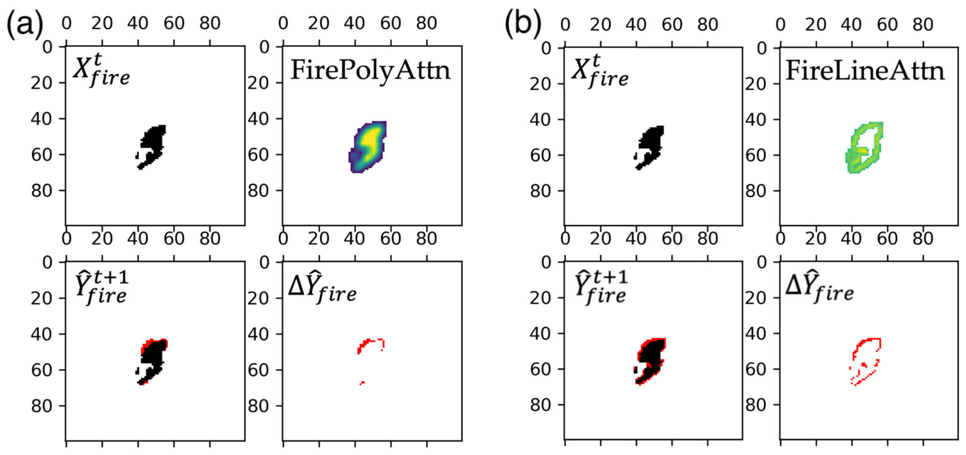
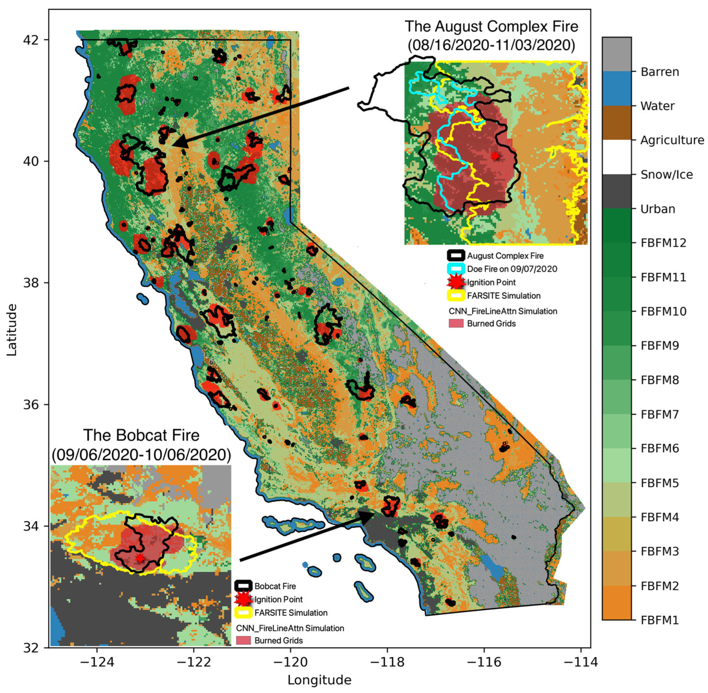
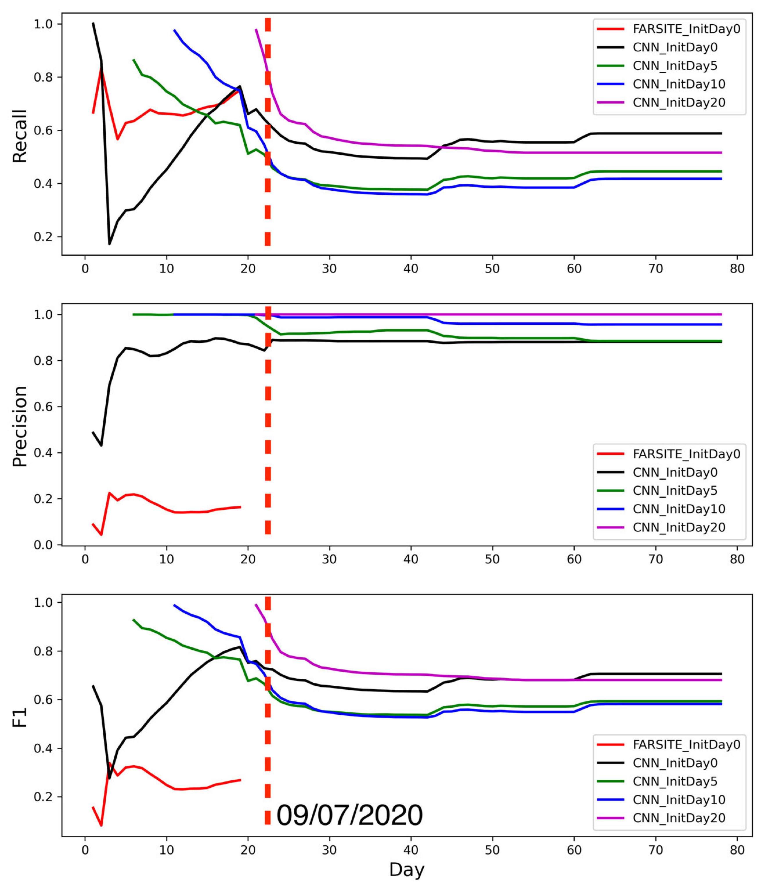
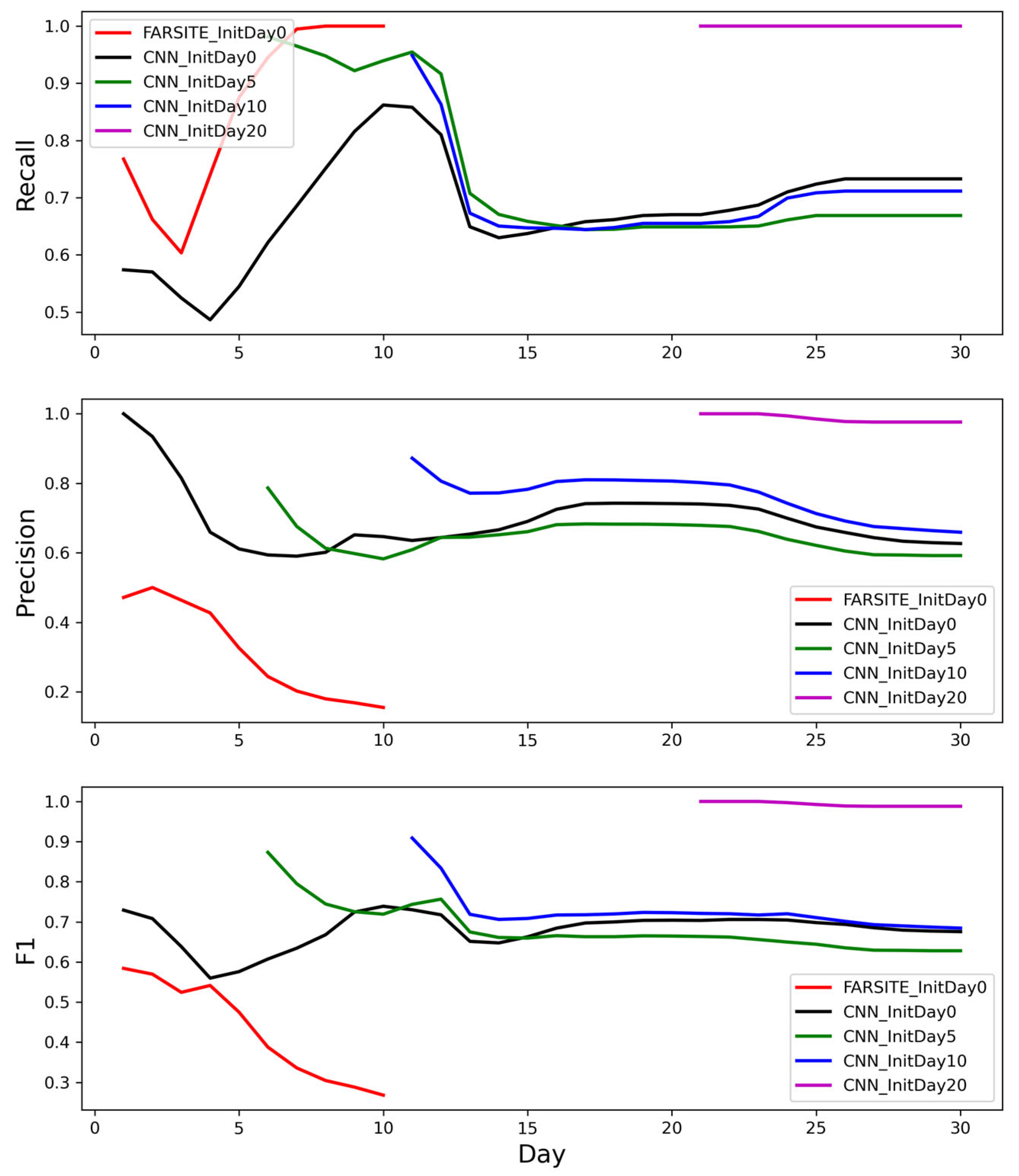
3.2. Spatial Distributions and Temporal Variations in Fire Simulations

The 2020 fire season resulted in nearly 10,000 registered fires and a total burned area of 17,419 km2, a record high in California’s modern history since the 1800s [34]. Here, we compare our recursive fire prediction results to the 103 large wildfires recorded by the VIIRS fire-tracking dataset in 2020. These wildfires lasted at least 2 days, with final fire sizes of no less than 4 km2. Additionally, we select two large wildfires to showcase the modeling performance of daily fire progression throughout the entire life cycle of each fire. The first example is the August Complex fire in northern California, which is a fire complex consisting of more than 30 individual fires. The August Complex fire and its main component, the Doe fire, are the largest fire complex and the single-largest wildfire in California’s recorded history, respectively, and they burned more than 4000 km2 in three months [35]. The second example is the Bobcat fire in southern California, which is one of the largest fires on record in Los Angeles County and burned more than 460 km2 [36].
Figure 5 illustrates the comparison of the final fire polygons of the 103 large wildfires in 2020 based on the VIIRS satellite observations and the CNN model simulations. The insets in the figure provide an enlarged view of the comparison between the CNN and FARSITE model simulations for the two selected large wildfire examples. Note that the August Complex fire originated as multiple separate fires initiated by lightning strikes on 16–17 August 2020, while the corresponding FARSITE and CNN fire simulations were initialized from a single ignition point (the red star in Figure 5) on the first day of the Doe fire as the main component of the August Complex fire. The CNN fire simulation extended for the same duration as the VIIRS observations to capture the entire length of the fires, while the FARSITE simulation for the August Complex fire was limited to the first 20 days. This is because the FARSITE simulation (the yellow line in Figure 5) produced results that were considerably larger than the observations, even surpassing the boundary of the 100 km × 100 km model domain after this time period. To ensure a fair comparison with the fire simulations, the perimeter of the Doe fire on 7 September 2020, prior to its merging with other fires such as the Elkhorn fire and the Hopkins fire of the fire complex, is also depicted on the map (the cyan line in Figure 5). After fire merging, the observed final burn scar of the August Complex fire exceeds the boundary of the 100 km × 100 km tile centered around the ignition point of the Doe fire. This can be solved by beginning fire simulations from each ignition point of the individual fires of the fire complex in practical applications.
Considering the extensive occurrence of fires throughout California, the 103 wildfires selected for the model evaluation exhibit diverse burning conditions in terms of fuel types, terrain, and weather. For example, the dominant vegetation type in the August Complex fire region is a Mediterranean California mesic mixed conifer forest and woodland, which is mainly characterized by quick surface and ground fires with frequent crowning and spotting causing difficulties for fire control (FBFM10). In comparison, the dominant vegetation types in the Bobcat fire region are southern California dry mesic chaparral and mixed evergreen woodland, which are mainly characterized by low intensity surface fires (FBFM5). Such diversity poses great challenges for the fire spread model in effectively learning various fire behavior and progression characteristics. Figure 5 shows that the CNN model generally captures the spatial patterns of most of the fires in 2020, with relatively larger discrepancies for those fires with larger sizes. This might be attributable to larger accumulative biases as all the recursive fire simulations begin from the ignition day of each fire. The large modeling biases are more significant in the FARSITE simulation results for the two large wildfire examples shown in the insets. The FARSITE final perimeters are much larger than both the CNN simulations and the VIIRS observations, especially in the August Complex fire simulation that exceeds the boundary of the model domain. Considering the much shorter simulation length of the FARSITE model, these results imply an overestimation of the fire spread rates in the FARSITE model. Moreover, the actual simulation cost of FARSITE is also significantly higher than the CNN model. FARSITE took 1020 s and 366 s to finish the 20-day simulation of the August Complex fire and the 10-day simulation of the Bobcat fire, respectively, which are 2~3 orders of magnitude slower than the CNN model. The much higher computational efficiency of the CNN model is essential for massive fire event simulations and fire risk assessments using the Monte Carlo approach.
To illustrate the temporal variations in modeling performance during fire progression, we also present the time series of the three metric scores throughout the simulations of the two large wildfire examples (Figure 6 and Figure 7). In order to further examine the influence of model initialization on the simulation results, the time series of the CNN model was started on different initialization days, including the ignition day (day 0), the fifth day (day 5), the tenth day (day 10), and the twentieth day (day 20) after ignition. For comparison, the time series of the FARSITE simulations starting from the ignition day (day 0) are also included. The results show drastically fluctuating modeling scores during the early stage of fire progression. This might result from rapid expansion and eruptive fire behavior during the early fire growth stage. Then, the fluctuations in these scores gradually become less volatile and flatten out in the end. This change can be attributed to relatively stable fire behavior due to human suppression or natural burnout during the late stage.
In the August Complex fire example, the recall and precision scores of the CNN model vary in a negatively correlated way during the first few days after ignition. Its recall score then recovers quickly, while its precision score remains relatively stable. Such nonlinear fluctuations in recall and precision lead to the highest peak at around 20 days in its F-1 score as the combination of the above two scores. Note that this peaking time coincides well with the merging time of the Doe fire with other separate fire incidents of the August Complex fire. Since the ignition points for the other fires in the fire complex are missing in this simulation, the modeling performance degrades gradually and finally becomes stable after the first 30 days since the ignition of the Doe fire. This is consistent in all the time series that began on different initialization days, although the modeling scores, especially the precision scores, are slightly higher in those simulations that were started on later initialization days, like day 20, due to their more precise model inputs from the later fire observations. In comparison, the metric scores of the FARSITE model show overestimated results that are consistent with its spatial pattern, characterized by relatively high recall scores but much lower precision and F-1 scores throughout its simulation.
In the Bobcat fire case, the results are similar to the August Complex fire except for the greatly improved modeling performance in the simulation initialized on day 20. The simulations initialized before day 20 all show nonlinear large fluctuations in modeling scores that reach similar stable levels after the first thirteen days. This change suggests fairly slow rates of fire spread due to minimal active burning during the later stage of the fire. The highest scores in the simulation initialized on day 20 are attributed to the most up-to-date model input of the initial fire polygon during this fire decay stage. In comparison, the FARSITE model achieves the highest recall score of 1 at a cost of continuously decreasing the precision and F-1 scores after the first seven days, suggesting an overestimated fire simulation result that is consistent with its spatial pattern in Figure 5.

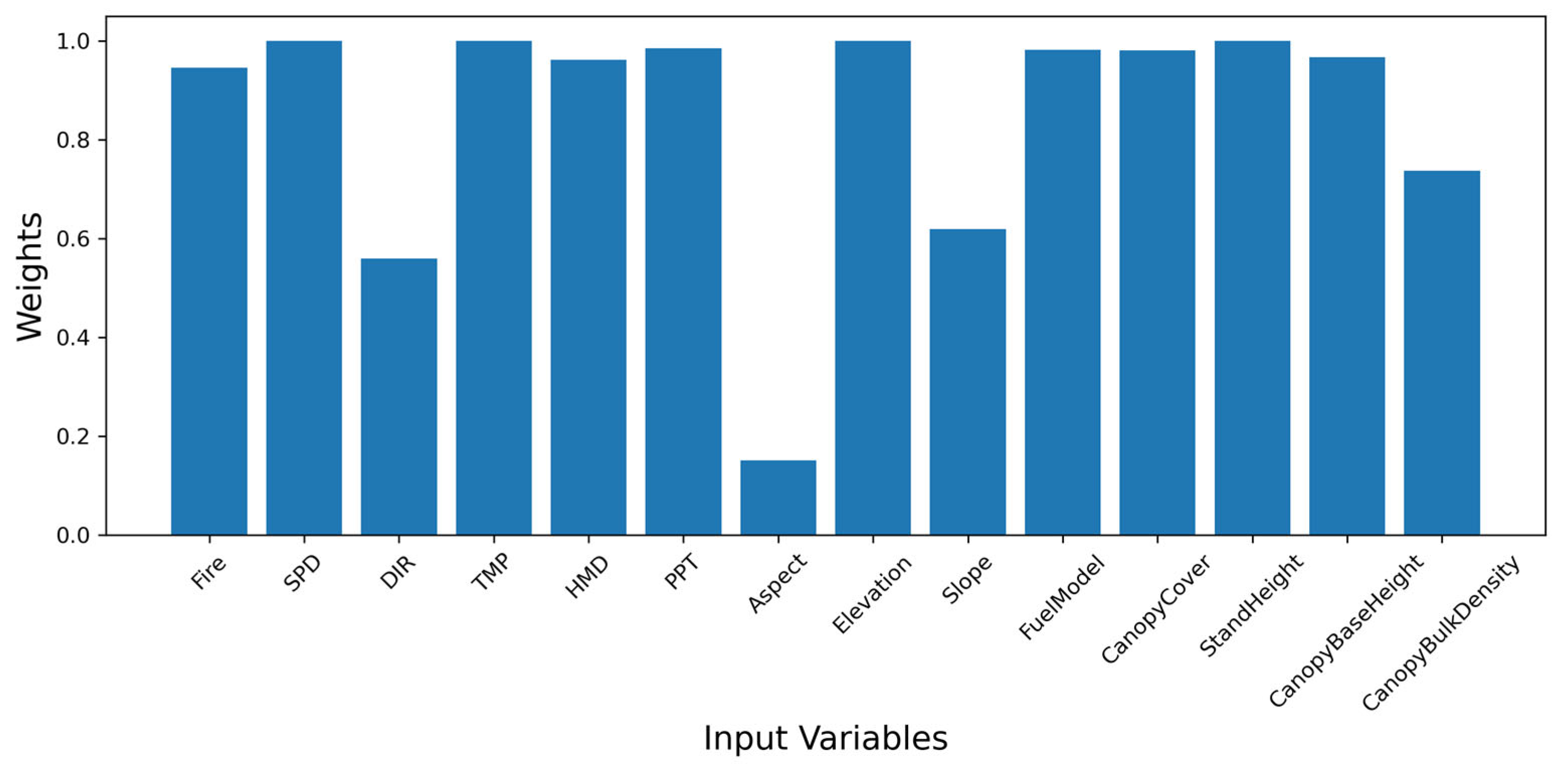
3.3. Feature Importance of Fire Simulations

The evaluation results presented above clearly demonstrate the benefits of incorporating the attention modules into the CNN fire spread models for modeling complete fire events through recursive prediction. Moreover, these attention modules also improve the model interpretability, which was often limited in previous date-driven fire models. By applying spatial and channel attention, the weights assigned to each model input feature can dynamically adapt to highlight critical spatial regions and channels as fire shapes change during fire progression, effectively minimizing the loss function. Therefore, the values of these weights can be interpreted as the relative importance or significance of each feature in influencing the modeling accuracy of the attention-based fire spread models. Larger weights indicate a higher degree of importance of the corresponding input features in specific regions, while smaller weights indicate a lesser degree of importance.
While the interpretation of channel-wise and spatial-wise attention weights in our attention-based fire spread models is generally consistent with that in the CBAM, there is a key difference in the spatial attention modules. In our models, the locations with positive spatial weights were pre-designed and prescribed based on an input fire perimeter map in the fire attention modules (see examples in Figure 3) rather than dynamically learned, as in the CBAM. This improvement was motivated by the understanding of physical fire spread processes because fire spread is more significantly influenced by localized environmental conditions around actively burning areas as opposed to remote conditions.
Regarding channel-wise attention, Figure 8 shows the averaged weights for each input feature of the CNN model based on the 103 wildfires in 2020. Initially, all input variables had equal weights of one, indicating no discrimination. However, during model training, the model adjusted these weights to minimize the loss function. It is observed that aspect has the lowest weight, followed by wind direction, slope, and canopy bulk density (Figure 8). The remaining input variables have similar weights that are close to the default value of one. While all the aforementioned factors associated with local terrain, fuel, and weather conditions can influence fire spread, it is challenging for the model to learn the complex effects of these variables at finer scales due to the relatively coarse model resolution of 1 km. The downscaled resolution of 1 km smooths out the fine details of terrain variables such as aspect and slope over complex terrains, potentially reducing their weights in the model to minimize the negative impact of noisy model inputs on fire simulations. Similarly, the moderate weight assigned to wind direction may be attributed to the limited capability of low-resolution raw data to accurately represent fine details of wind fields and their heterogeneous impacts on fire spread (see an example in Figure 1).

4. Discussion

The promising modeling results of recursive fire prediction demonstrate the high value of our attention-based fire spread models for practical applications such as short-term fire spread prediction and long-term fire risk assessment using the Monte Carlo approach. This improvement results from both the high-resolution fire-tracking dataset with abundant fire progression information for model training and the attention-based modeling architecture. Fire spread mainly occurs in actively burning regions such as fire frontlines, a factor which is captured well by the fire line attention module of our attention-based spread models to aid in learning continuous fire progression from high-resolution fire-tracking data.
As discussed earlier, the recently developed ML-/DL-based fire spread models [21,22,23,24] were primarily trained to predict fire spread over short timeframes (hours to days) rather than to simulate complete fire events. On the other hand, while traditional semi-empirical fire behavior models like FARSITE [15] and FlamMap [16] can simulate continuous fire progression at a higher spatiotemporal resolution, they have higher computational costs and require more model-tuning efforts to address potential modeling biases. It is noted that the considerably larger FARSITE simulation results may be attributed to the overdried fuel moisture estimates resulting from insufficient weather condition information from limited ground observation stations. Although these biases could be partially alleviated by manually adding fuel moisture adjustment factors in the FARSITE simulations, it is a heuristic and empirical approach to compensate. For a direct comparison between all model simulations, the optional fuel moisture adjustment factors were not used in the FARSITE simulations in this study. It is essential to note that the comparison with FARSITE was limited to two fire cases. Additionally, each of these models exhibits its unique advantages and disadvantages, and improved modeling performance can be achieved via fine-tuning in both semi-empirical and data-driven fire models, making them suitable for various practical applications based on specific needs.
The attention-based fire spread models, particularly the one incorporating the fire line attention module, as proposed in this study, achieve both balanced modeling performance and high computational efficiency in simulating complete fire events. This capability is highly advantageous for practical applications such as active fire prediction and fire risk assessment. However, the current 1 km model resolution is insufficient for accurately assessing fine-scale fire risks at the property level. In the future, the data-driven fire models can be further improved by taking the following steps:
(1)
Increasing the sample size and resolution for model training and testing. Currently, there are 735 fires from 2012 to 2020 available for model training and evaluation. Although this dataset can be augmented by data rotation, more training samples at higher spatiotemporal resolutions across more diversified landscapes and fire regimes could benefit the improvement of modeling performance, as we saw in the experiments of this study. Meanwhile, the data quality of the corresponding fuel, terrain, and weather conditions influencing fire spread should also be improved to provide sufficient information for models to learn complex fire behavior.
(2)
Adding new features as model inputs to take into account human effects on fire control and suppression. The model inputs considered in this study are natural factors representing terrain, fuel, and weather conditions. However, human activity and land segmentation such as road and stream networks can also affect fire spread in multiple ways. The human suppression effect is particularly significant in WUI areas given the high prioritization of protecting people via firefighting activities. Currently, such a suppression effect is implicitly learned by the model from observed fire progression. More explicit model input features associated with human effects might further improve the modeling capability in this regard.
(3)
Refining the model architectures with improved model interpretability. The current attention modules, especially the fire line attention module, enable the model to focus on actively burning areas that are critical for fire spread. This learning approach is also consistent with actual burning processes guided by the laws of combustion chemistry and physics. Further refinement can be informed by a more comprehensive consideration of nonlinear physical fire progression processes in the model to improve modeling performance and interpretability simultaneously.
(4)
Integrating the model with other complementary models, such as fire ignition [37], duration, and vulnerability models, for comprehensive fire risk assessment. Recognizing that fire spread is part of the entire burning process, it is essential to incorporate this model into a broader modeling framework to simulate complete fire events, encompassing all burning processes from ignition to burnout. This integrated modeling approach allows for scenario analysis in short-term fire spread prediction and fire risk assessment at broader spatiotemporal scales, such as generating large numbers of simulated fire events using Monte Carlo approaches and estimating fire losses with a consideration for spatially heterogeneous vulnerability. Given the scarcity of extreme fire events in observed history, this capability to model catastrophic extreme events is particularly beneficial for tail risk analysis in the insurance industry.

5. Conclusions

We have developed multiple fire spread models that incorporate various attention mechanisms and conducted a comprehensive evaluation for both next-step prediction and recursive prediction. The attention-based CNN models were compared to a deeper and more complex autoencoder model and the widely used semi-empirical FARSITE fire behavior model in terms of computational accuracy and efficiency. The evaluation results demonstrate that the inclusion of the attention modules and data augmentation techniques significantly improves the modeling performance of the CNN models. Among the models tested, the CNN model with the fire line attention module, which was trained using augmented input data, achieved the most balanced performance, as measured by the F-1 and PR-AUC scores. This highlights the effectiveness of the attention mechanism in capturing complex fire behavior across diverse landscapes and fire regimes. These attention-based fire spread models provide a solid foundation for various applications, including short-term fire spread prediction and long-term fire risk assessment, to enhance fire risk assessment and management capabilities.

Author Contributions

Conceptualization, Y.Z., Y.L. and S.L.; methodology, Y.Z.; software, Y.Z. and A.P.; validation, Y.Z. and M.S.; data curation, Y.Z., M.S., Y.C. and N.A.; data analysis, Y.Z., M.S., Y.L., Y.C., N.A. and P.G.; writing—original draft preparation, Y.Z.; writing—review and editing, Y.L., Y.C. and N.A.; visualization, Y.Z.; project administration, S.L. All authors have read and agreed to the published version of the manuscript.

Funding

This research received no external funding.

Institutional Review Board Statement

Not applicable.

Informed Consent Statement

Not applicable.

Data Availability Statement

The VIIRS FEDS data used for model training and evaluation are available on figshare at https://doi.org/10.6084/m9.figshare.c.5601537.v1 (accessed on 31 May 2022). The fuel and terrain data used for model training are available on the LANDFIRE website: https://landfire.gov (accessed on 10 March 2022). The NEXGDM and ERA5 weather data used for model training are available on the NASA GeoNEX data portal website: https://data.nas.nasa.gov/geonex/geonexdata/NEX-GDM/ (accessed on 10 March 2022) and the Copernicus Climate Change Service (C3S) Climate Data Store (CDS) website: https://cds.climate.copernicus.eu/cdsapp#!/dataset/reanalysis-era5-single-levels?tab=overview (accessed on 10 March 2022), respectively.

Acknowledgments

We are thankful to the editors and three reviewers for their constructive comments and suggestions to improve the quality of the manuscript.

Conflicts of Interest

The authors declare no conflict of interest.

Appendix A

All the CNN models in this work were developed in the Keras API of TensorFlow 2.8. Figure A1, Figure A2 and Figure A3 show graphs of the model architectures for all the three CNN models in the main text.
Figure A1. The graph of the CNN_NonAttn model.
Fire 06 00289 g0a1
Figure A2. The graph of the CNN_FirePolyAttn model.
Fire 06 00289 g0a2
Figure A3. The graph of the CNN_FireLineAttn model.
Fire 06 00289 g0a3
Both the CNN_FirePolyAttn and CNN_FireLineAttn models share the same channel attention module, which was computed in the same way as in Woo et al., 2016 [31], as follows:
M c F = σ ( M L P A v g P o o l F + M L P ( M a x P o o l ( F ) ) ) ,
where M c R C × 1 × 1 is a 1D channel attention map, F R C × H × W is a 3D input feature map, σ denotes the sigmoid function, A v g P o o l and M a x P o o l denote the average and max pooling operations, and M L P denotes a shared network composed of a multi-layer perceptron with one hidden layer.
In the CNN_FirePolyAttn model, the 2D fire polygon attention map M f i r e _ p o l y R 1 × H × W is computed as follows:
M f i r e _ p o l y F f i r e t 1 = σ A v g P o o l F f i r e t 1 ,
where F f i r e t 1 R 1 × H × W is a 2D binary fire feature map generated from the last timestep as input, and σ denotes a rescaling function that rescales the weights into the [0, 1] range.
In the CNN_FireLineAttn model, the 2D fire line attention map M f i r e _ l i n e R 1 × H × W is computed as follows:
M f i r e _ l i n e F f i r e t 1 = σ A v g P o o l F f i r e t 1 A v g P o o l 1 F f i r e t 1 ,
where denotes element-wise multiplication, and F f i r e t 1 and σ are the same as in M f i r e _ p o l y .
After obtaining these attention maps, we then multiply them with input feature maps ( F ) sequentially to generate refined feature maps ( F ) as follows:
F = M c F F ,   F = M f i r e _ p o l y F f i r e t 1 F   or   F = M f i r e _ l i n e F f i r e t 1 F .
In addition to the CNN models, we also used a persistent model, an autoencoder model [24], and the FARSITE fire behavior model [15] for model comparison and benchmarking. The persistent model is simple and straightforward and assumes unchanging fire shapes between two consecutive timesteps, which leads to identical fire polygons throughout its simulation. The autoencoder model first encodes the input features into a bottleneck feature representation and then decodes them through up-sampling. We used the same number of filters (32, 64, 128, 256, 256) as the modeling setting selected in Huot et al. [24]. The 100 × 100 pixel input features were cropped to 96 × 96 pixel tiles by dropping the two pixels around the boundary of the input images for down-sampling and up-sampling in the autoencoder model. We then trained and evaluated this autoencoder model in the same way as the CNN models. The FARSITE model is different from the other models implemented in this study because it is a two-dimensional semi-empirical model that simulates fire growth and the behavior of surface and crown fires based on Huygen’s principle of wave propagation and the Rothermel fire spread equations. The spotting feature was disabled in the FARSITE simulations in this study. To simulate the two large wildfires in the main text, we used the LANDFIRE terrain and fuel input data at the original 30 m resolution for FARSITE simulations. The weather inputs were prepared based on the in-situ observations of the two remote automatic weather stations (RAWSs) closest to the two fires (the Mendocino Pass station for the August Complex fire and the Tanbark station for the Bobcat fire).
After the model simulations, we used the confusion matrix in Table A1 to calculate metric scores for model evaluation. These scores were calculated for each timestep of the 103 fires in 2020 after their ignition days. The average scores for final timesteps of these fires are listed in Table 1 of the main text, while the average scores for all timesteps of the same fires are listed in Table A2 herein.
Table A1. Confusion matrix for the binary classification of fire prediction in this study.
Prediction TruthPrediction False
Ground truthTPFN
Ground falseFPTN
Table A2. The averaged evaluation results of fire spread models in next-step and recursive prediction for all timesteps of the 103 wildfires in 2020. The highest scores for each metric are highlighted in bold.
MetricsModel
Parameters
Next-Step PredictionRecursive Prediction
Model NameRecallPrecisionF-1RecallPrecisionF-1
Autoencoder5.5M0.680.720.650.380.740.40
CNN_NonAttn8.8k0.671.00.710.080.980.13
CNN_FirePolyAttn12k0.840.860.810.490.670.43
CNN_FireLineAttn12k0.900.690.710.630.510.41
CNN_FirePolyAttn_R *12k0.820.870.810.450.710.43
CNN_FireLineAttn_R *12k0.880.710.740.700.460.47
* Models trained with augmented input data via data rotation.

References

  1. Dennison, P.E.; Brewer, S.C.; Arnold, J.D.; Moritz, M.A. Large wildfire trends in the western United States, 1984–2011. Geophys. Res. Lett. 2014, 41, 2928–2933. [Google Scholar] [CrossRef]
  2. Iglesias, V.; Balch, J.K.; Travis, W.R. US fires became larger, more frequent, and more widespread in the 2000s. Sci. Adv. 2022, 8, eabc0020. [Google Scholar] [CrossRef]
  3. Strader, S.M. Spatiotemporal changes in conterminous US wildfire exposure from 1940 to 2010. Nat. Hazards 2018, 92, 543–565. [Google Scholar] [CrossRef]
  4. Burke, M.; Driscoll, A.; Heft-Neal, S.; Xue, J.; Burney, J.; Wara, M. The changing risk and burden of wildfire in the United States. Proc. Natl. Acad. Sci. USA 2021, 118, e2011048118. [Google Scholar] [CrossRef] [PubMed]
  5. Zhuang, Y.; Fu, R.; Santer, B.D.; Dickinson, R.E.; Hall, A. Quantifying contributions of natural variability and anthropogenic forcings on increased fire weather risk over the western United States. Proc. Natl. Acad. Sci. USA 2021, 118, e2111875118. [Google Scholar] [CrossRef] [PubMed]
  6. Westerling, A.L.; Hidalgo, H.G.; Cayan, D.R.; Swetnam, T.W. Warming and earlier spring increase western US forest wildfire activity. Science 2006, 313, 940–943. [Google Scholar] [CrossRef] [PubMed] [Green Version]
  7. Abatzoglou, J.T.; Williams, A.P. Impact of anthropogenic climate change on wildfire across western US forests. Proc. Natl. Acad. Sci. USA 2016, 113, 11770–11775. [Google Scholar] [CrossRef] [Green Version]
  8. Williams, A.P.; Abatzoglou, J.T.; Gershunov, A.; Guzman-Morales, J.; Bishop, D.A.; Balch, J.K.; Lettenmaier, D.P. Observed impacts of anthropogenic climate change on wildfire in California. Earth’s Future 2019, 7, 892–910. [Google Scholar] [CrossRef] [Green Version]
  9. Balch, J.K.; Bradley, B.A.; Abatzoglou, J.T.; Nagy, R.C.; Fusco, E.J.; Mahood, A.L. Human-started wildfires expand the fire niche across the United States. Proc. Natl. Acad. Sci. USA 2017, 114, 2946–2951. [Google Scholar] [CrossRef]
  10. Radeloff, V.C.; Helmers, D.P.; Kramer, H.A.; Mockrin, M.H.; Alexandre, P.M.; Bar-Massada, A.; Butsic, V.; Hawbaker, T.J.; Martinuzzi, S.; Syphard, A.D. Rapid growth of the US wildland-urban interface raises wildfire risk. Proc. Natl. Acad. Sci. USA 2018, 115, 3314–3319. [Google Scholar] [CrossRef] [Green Version]
  11. Busenberg, G. Wildfire management in the United States: The evolution of a policy failure. Rev. Policy Res. 2004, 21, 145–156. [Google Scholar] [CrossRef]
  12. Moritz, M.A.; Batllori, E.; Bradstock, R.A.; Gill, A.M.; Handmer, J.; Hessburg, P.F.; Leonard, J.; McCaffrey, S.; Odion, D.C.; Schoennagel, T.; et al. Learning to coexist with wildfire. Nature 2014, 515, 58–66. [Google Scholar] [CrossRef] [PubMed]
  13. Sullivan, A.L. Wildland surface fire spread modelling, 1990–2007. 1: Physical and quasi-physical models. Int. J. Wildland Fire 2009, 18, 349–368. [Google Scholar] [CrossRef] [Green Version]
  14. Sullivan, A.L. Wildland surface fire spread modelling, 1990–2007. 2: Empirical and quasi-empirical models. Int. J. Wildland Fire 2009, 18, 369–386. [Google Scholar] [CrossRef] [Green Version]
  15. Finney, M.A. FARSITE, Fire Area Simulator—Model Development and Evaluation; Research Paper RMRS-RP-4; US Department of Agriculture, Forest Service, Rocky Mountain Research Station: Fort Collins, CO, USA, 1998.
  16. Finney, M.A. An Overview of FlamMap Fire Modeling Capabilities. In Fuels Management—How to Measure Success: Conference Proceedings; Andrews, P.L., Butler, B.W., Eds.; U.S. Department of Agriculture, Forest Service, Rocky Mountain Research Station: Fort Collins, CO, USA, 2006; pp. 213–220. [Google Scholar]
  17. Li, F.; Levis, S.; Ward, D.S. Quantifying the role of fire in the Earth system—Part 1: Improved global fire modeling in the Community Earth System Model (CESM1). Biogeosciences 2013, 10, 2293–2314. [Google Scholar] [CrossRef] [Green Version]
  18. Lautenberger, C. Wildland fire modeling with an Eulerian level set method and automated calibration. Fire Saf. J. 2013, 62, 289–298. [Google Scholar] [CrossRef]
  19. Mandel, J.; Beezley, J.D.; Kochanski, A.K. Coupled atmosphere-wildland fire modeling with WRF 3.3 and SFIRE 2011. Geosci. Model Dev. 2011, 4, 591–610. [Google Scholar] [CrossRef] [Green Version]
  20. Jiang, W.L.; Wang, F.; Fang, L.; Zheng, X.; Qiao, X.; Li, Z.; Meng, Q. Modelling of wildland-urban interface fire spread with the heterogeneous cellular automata model. Environ. Model. Softw. 2021, 135, 104895. [Google Scholar] [CrossRef]
  21. Hodges, J.L.; Lattimer, B.Y. Wildland fire spread modeling using convolutional neural networks. Fire Technol. 2019, 55, 2115–2142. [Google Scholar] [CrossRef]
  22. Radke, D.; Hessler, A.; Ellsworth, D. FireCast: Leveraging Deep Learning to Predict Wildfire Spread. In Proceedings of the IJCAI 2019, Macao, China, 10–16 August 2019. [Google Scholar]
  23. Khennou, F.; Ghaoui, J.; Akhloufi, M.A. Forest fire spread prediction using deep learning. In Proceedings of the Geospatial Informatics XI, Online, 12–17 April 2021; p. 11733. [Google Scholar]
  24. Huot, F.L.; Hu, R.L.L.; Ihme, M.; Wang, Q.; Burge, J.; Lu, T.; Hickey, J.; Chen, Y.F.; Anderson, J. Deep learning models for predicting wildfires from historical remote-sensing data. arXiv 2021, arXiv:2010.07445v3. [Google Scholar]
  25. Chen, Y.; Hantson, S.; Andela, N.; Coffield, S.R.; Graff, C.A.; Morton, D.C.; Ott, L.E.; Foufoula-Georgiou, E.; Smyth, P.; Goulden, M.L.; et al. California wildfire spread derived using VIIRS satellite observations and an object-based tracking system. Sci. Data 2022, 9, 249. [Google Scholar] [CrossRef] [PubMed]
  26. LANDFIRE Topographic Products. Available online: https://landfire.gov/topographic.php (accessed on 10 March 2022).
  27. LANDFIRE Fuel Products. Available online: https://landfire.gov/fuel.php (accessed on 10 March 2022).
  28. Hashimoto, H.; Wang, W.; Melton, F.S.; Moreno, A.L.; Ganguly, S.; Michaelis, A.R.; Nemani, R.R. High-resolution mapping of daily climate variables by aggregating multiple spatial data sets with the random forest algorithm over the conterminous United States. Int. J. Climatol. 2019, 39, 2964–2983. [Google Scholar] [CrossRef]
  29. NASA GeoNEX Data Portal. Available online: https://data.nas.nasa.gov/geonex/geonexdata/NEX-GDM/ (accessed on 10 March 2022).
  30. Hersbach, H.; Bell, B.; Berrisford, P.; Biavati, G.; Horányi, A.; Muñoz Sabater, J.; Nicolas, J.; Peubey, C.; Radu, R.; Rozum, I.; et al. ERA5 Hourly Data on Single Levels from 1940 to Present. Copernicus Climate Change Service (C3S) Climate Data Store (CDS). 2023. Available online: https://cds.climate.copernicus.eu/cdsapp#!/dataset/reanalysis-era5-single-levels?tab=overview (accessed on 10 March 2022).
  31. Woo, S.; Park, J.; Lee, J.Y.; Kweon, I.S. CBAM: Convolutional block attention module. In Proceedings of the European Conference on Computer Vision (ECCV) 2018, Munich, Germany, 8–14 September 2018. [Google Scholar]
  32. Branco, P.; Torgo, L.; Ribeiro, R.P. A survey of predictive modeling on imbalanced domains. ACM Comput. Surv. (CSUR) 2016, 49, 1–50. [Google Scholar] [CrossRef] [Green Version]
  33. Abraham, N.; Khan, N.M. A novel focal tversky loss function with improved attention u-net for lesion segmentation. In Proceedings of the 2019 IEEE 16th International Symposium on Biomedical Imaging (ISBI 2019), Venice, Italy, 8–11 April 2019. [Google Scholar]
  34. Safford, H.D.; Paulson, A.K.; Steel, Z.L.; Young, D.J.; Wayman, R.B. The 2020 California fire season: A year like no other, a return to the past or a harbinger of the future? Glob. Ecol. Biogeogr. 2022, 31, 2005–2025. [Google Scholar] [CrossRef]
  35. August Complex Fire. Available online: https://en.wikipedia.org/wiki/August_Complex_fire (accessed on 24 January 2023).
  36. Bobcat Fire. Available online: https://en.wikipedia.org/wiki/Bobcat_Fire (accessed on 24 January 2023).
  37. Liu, Y.; Le, S.; Zou, Y.; Sadgedhi, M.; Chen, Y.; Andela, N.; Gentine, P. A Simplified Machine Learning Based Wildfire Ignition Model from Insurance Perspective. In ICLR 2023 Workshop on Tackling Climate Change with Machine Learning. 2023. Available online: https://www.climatechange.ai/papers/iclr2023/23 (accessed on 20 June 2023).
Figure 1. Examples of processed model input data for the Bobcat fire 10 days after its ignition. SPD: wind speed; DIR: wind direction, TMP: maximum air temperature; HMD: relative humidity; PPT: precipitation. The FuelModel variable represents distributions of fuel loading among surface fuel components, size classes, and fuel types. Note that there is no precipitation in this example, and DIR has a much coarser resolution than other input features.
Fire 06 00289 g001
Figure 2. Model architectures of the attention-based fire spread models. The fire attention modules are illustrated in the boxes.
Fire 06 00289 g002
Figure 3. Examples of fire prediction using different attention modules. (a) CNN_FirePolyAttn with the fire polygon attention module (top-right) that uses X f i r e t (top-left) to predict Y ^ f i r e t + 1 (bottom-left) directly. Y ^ f i r e (bottom-right) is derived by subtracting X f i r e t from Y ^ f i r e t + 1 in this case; (b) CNN_FireLineAttn, with the fire line attention module (top-right) that first uses X f i r e t (top-left) to predict Y ^ f i r e (bottom-right) and then derives Y ^ f i r e t + 1 (bottom-left) by adding Y ^ f i r e to X f i r e t . In both (a,b), the black color denotes burned fire pixels, the red color highlights the fire pixel changes between X f i r e t and Y ^ f i r e t + 1 , and the color gradient denotes spatial weights in the two fire attention modules.
Fire 06 00289 g003
Figure 4. Histograms of the recall, precision, and F-1 scores of the CNN_FireLineAttn models trained without (top) and with (bottom) data augmentation for the recursive prediction of the final fire polygons of the 103 wildfires in 2020.
Fire 06 00289 g004
Figure 5. Comparison of final fire perimeters from the VIIRS satellite observations (black lines) and the CNN_FireLineAttn_R simulations (red polygons) for the 103 wildfires in 2020. Two examples of large wildfires, the August Complex fire and the Bobcat fire, with corresponding ignition points (red stars), intermediate VIIRS observations (cyan lines), FARSITE simulations (yellow lines), and FBFM fuel models (color shading) are enlarged in the insets, respectively. FBFM1–12 represent different fuel types in the 13 Anderson Fire Behavior Fuel Models.
Fire 06 00289 g005
Figure 6. Time series of recall, precision, and F-1 scores of the August Complex fire simulations by the FARSITE and CNN models initialized with fire observations on different days. The red dashed line denotes the date before the Doe fire merged with the Elkhorn fire and the Hopkins fire (see the cyan polygons in Figure 5).
Fire 06 00289 g006
Figure 7. Time series of recall, precision, and F-1 scores of the Bobcat fire simulations by the FARSITE and CNN models initialized with fire observations on different days.
Fire 06 00289 g007
Figure 8. The averaged weights for the model input variables in the channel attention module.
Fire 06 00289 g008
Table 1. The averaged evaluation results of fire spread models in both next-step and recursive prediction for final fire perimeters of the 103 wildfires in 2020. The highest scores for each metric are highlighted in bold.
MetricsModel
Parameters
Next-Step PredictionRecursive Prediction
Model NameRecallPrecisionF-1PR-AUCRecallPrecisionF-1PR-AUC
Persistent model00.791.00.82N/A **0.041.00.08N/A **
Autoencoder5.5 M0.710.740.690.600.310.760.380.06
CNN_NonAttn8.8 k0.791.00.820.980.040.990.080.03
CNN_FirePolyAttn12 k0.880.930.890.980.400.720.410.07
CNN_FireLineAttn12 k0.910.810.830.950.550.570.420.08
CNN_FirePolyAttn_R *12 k0.870.930.890.980.350.760.390.06
CNN_FireLineAttn_R *12 k0.900.790.820.920.670.440.450.24
* Models trained with augmented input data via data rotation. ** Not available.
Disclaimer/Publisher’s Note: The statements, opinions and data contained in all publications are solely those of the individual author(s) and contributor(s) and not of MDPI and/or the editor(s). MDPI and/or the editor(s) disclaim responsibility for any injury to people or property resulting from any ideas, methods, instructions or products referred to in the content.

