Article

Field-Scale Physical Modelling of Grassfire Propagation on Sloped Terrain under Low-Speed Driving Wind

by
Jasmine Innocent
1,
Duncan Sutherland
2 and
Khalid Moinuddin
1,*
1
Institute for Sustainable Industries and Liveable Cities, Victoria University, Melbourne, VIC 3030, Australia
2
School of Science, University of New South Wales, Canberra, ACT 2610, Australia
*
Author to whom correspondence should be addressed.
Fire 2023, 6(10), 406; https://doi.org/10.3390/fire6100406
Submission received: 3 July 2023 / Revised: 4 October 2023 / Accepted: 10 October 2023 / Published: 20 October 2023
(This article belongs to the Special Issue Understanding and Managing Extreme Wildland Fires)

Abstract

:
Driving wind and slope of terrain can increase the rate of surface fire propagation. Previous physical modelling under higher driving wind (3–12.5 m/s) on slopes (Innocent et al., IJWF, 2023, 32(4), pp. 496–512 and 513–530) demonstrated that the averaged rate of fire spread (RoS) varied from that of empirical models. This study investigates the potential for better agreement at lower wind velocities (0.1 and 1 m/s), since empirical models are typically developed from experimental studies conducted under benign wind conditions. The same physical model WFDS is used. The results are analysed to understand the behaviour of various parameters (RoS, fire isochrone progression, fire intensity, flame dynamics, and heat fluxes) across different slopes. The RoS–slope angle relationship closely fits an exponential model, aligning with the findings from most experimental studies. The relative RoSs are aligned more closely with the Australian and Rothermel models’ slope corrections for 0.1 and 1 m/s, respectively. The relationship between flame length and fire intensity matches predictions from an empirical power–law correlation. Flame and plume dynamics reveal that the plume rises at a short distance from the ignition line and fire propagation is primarily buoyancy-driven. The Byram number analysis shows buoyancy-dominated fire propagation at these lower wind velocities. Convective heat fluxes are found to be more significant at greater upslopes. The study confirmed that “lighter & drier” fuel parameters accelerated the fire front movement, increasing the RoS by approximately 57–60% compared to the original parameters. Overall, this study underscores the nuanced interplay of wind speed, slope, and other factors in influencing grassfire behaviour, providing valuable insights for predictive modelling and firefighting strategies.

1. Introduction

Fire behaviour is influenced by various topographical, weather, and fuel parameters. Wind speed and terrain slope of the terrain are two major determinants of the rate of fire spread (RoS). The slope of the terrain can greatly affect fire behaviour, potentially increasing or decreasing the rate at which the fire spreads, depending on whether the slope ascends or descends. Wind is an important weather parameter that significantly impacts fire propagation. When wind and slope factors are combined, they can produce distinct variations in fire behaviour based on different combinations of the two. In our previous two-part paper [1,2], the effect of higher wind velocities (3, 6, and 12.5 m/s) on grassfire propagation on various sloped (−30° to +30°) terrain was investigated. In [1], the detailed motivation of the overall study is presented along with model set-up, validation studies, and sensitivity analysis. The comparisons of RoS with the existing empirical models on sloped terrain at higher wind velocities were presented in [1]. The present paper emphasizes the impact of lower wind speeds of 0.1 and 1 m/s on fire propagation on sloped terrain. In our study, we use a physical model WFDS (Wildland–Urban Interface Fire Dynamics Simulator), version 9977 [3], compatible with FDS (Fire Dynamic Simulator) version 6.0 [4]. Insight from three-dimensional physical modelling can enhance our understanding of fire propagation physics and contribute to refinement of the empirical and semi-empirical fire models used by fire and emergency services [3,5,6,7,8,9,10].
Empirical or semi-empirical models within operational platforms are commonly used to predict quasi-steady RoS in real time. Some models also estimate flame height and fire intensity. The RoS flat terrain influenced by driving wind, or on a slope without wind, serves as the baseline for these models. Then slope and/or wind corrections are either added or multiplied to obtain the RoS for sloped terrain. Commonly used empirical models based on Australian grassfire experiments for no slope, driven by wind, are the McArthur models MKIII and MKV [11,12] and the CSIRO model proposed by Cheney et al. [13]. Noble et al. [14] introduced equations for the Mark III and Mark V versions of McArthur’s grassland fire danger meter. The RoS is proposed as a function of the fire danger index (FDI), as presented in Equation (1).
R o S = C 1   f C , T , H , U 10 , W k m / h
where U 10 is the open wind speed at 10 m above the ground, T is the air temperature (°C), H is the relative humidity in percent, C is the curing index, W (tonnes/ha) is the fuel load, and C 1 is an empirical constant.
The CSIRO empirical fire spread model by Cheney et al. [13] incorporates a fuel load coefficient in determining RoS, which is given by Equation (2):
R o S = { 0.054 + 0.209 U 10 M C   , U 10 5   k m / h , 1.1 + 0.715 U 10 5 0.844 M C   , U 10 > 5   k m / h   }   ,
where M and C are the coefficients of fuel moisture and curing, respectively.
Further details of these models (Equations (1) and (2)) can be found in Moinuddin et al. [15]. These three models use a multiplicative slope correction [14], as shown in Equations (3) and (4).
Uphill ,   R o S c o r r = R o S   e 0.069 γ s  
Downhill ,   R o S c o r r = R o S   e 0.069   γ s
where RoS is the fire-spread rate involving only wind and R o S c o r r includes both wind and slope. γ s is the effective slope of the terrain expressed in degrees. These multiplicative models suggest an approximate doubling of RoS for every 10° increase in upslope. This correction is deemed valid up to ±20° slope [6,12].
The Rothermel surface fire spread model [16] is a semi-empirical model extensively used in US fire management systems. In the additive Rothermel models [16], the R o S c o r r is defined by Equation (5):
R o S c o r r = R o S 0   ( 1 + ϕ w i n d + ϕ s l o p e )
where R o S 0 is the fire spread rate when there is no wind and slope involved. ϕwind and ϕslope are the factors for wind and slope, respectively. This model is considered applicable up to 0–37° upslope angles. There are two versions of the Rothermel model—“original” and “modified” [17,18]. The packing ratio and surface-to-volume ratio are the two important components of the model for R o S 0 . The “modified” model incorporates an extinction index, which is a function of heat of vaporisation and fuel moisture content [18]. The details of R o S 0 , ϕwind, and ϕslope for Rothermel models can be found in [17,18,19]. The detailed equations for both “original” and “modified” models are presented in supplementary document, Annexure A.
In previous work [1], it was suggested that the traditional approach of calculating the rate of fire spread for a flat surface based on wind, and then adjusting for slope, might not be accurate. Observations in [1,2] highlighted dynamic fire behaviour especially when observing time series data of R o S (For simplicity, from now on, RoS is used for fire-spread rate irrespective of wind or slope involvement). The results of high velocity cases [1] indicated a second-order polynomial relationship between the quasi-steady R o S and slope angle, which was also the case when Rothermel RoS values were plotted against the slope. The slope factor in R o S c o r r in Australian empirical correlations (Equations (3) and (4)) appears to be exponential. These correlations likely stem from laboratory slope studies conducted under very low wind conditions. For upslopes, the slope factor (in terms of relative RoS values) simulated in WFDS more closely aligns with predictions from the Rothermel models than the Australian correlations.
In [1], we presented a comprehensive literature review. Since then, a few new studies have emerged. Cruz et al. [20] analysed a relatively large and diverse dataset of rate of fire spread observations and developed a rule of thumb, for swiftly assessing (in places where a fire behaviour prediction model may not be existent) the spread potential of grassfire burning under critical burning conditions. They estimated that the forward rate of spread is approximately 20% of the average 10 m open wind speed (U10). This 20% rule of thumb is likely to represent a worst- or near-worst-case scenario for fire spread where FMCs are low (<6%) and open winds are strong (>30 km/h). Bishe et al. [21] developed a two-dimensional quasi-physical model that examined heat transfer (radiative and convective) to predict a fire’s rate of spread on flat terrain. They also performed a comprehensive sensitivity analysis of their model to the major parameters (such as temperature, humidity, wind speed, specifications of fuel) that influence fire propagation. They validated the rate of spread results of their semi-physical model against the Australian grassland experiments F19 and C064 of Cheney et al. [22], and also compared their results with the WFDS results of Mell et al. [3]. However, these two studies did not include slope scenarios.
In our previous work [2], we also investigated flame characteristics, interactions between the plume and terrain, heat transfer mechanisms, and the mode of fire propagation. The flame and plume behaviour analysis for higher wind velocities in [2] demonstrated that the flame and near-flame appeared to be rising, even though the plume was attached. With higher wind velocities, flame behaviour could be different from the overall plume behaviour and the Byram number [23] based on U 10 captured the behaviour of plume, not the flame.
The Byram convection number, Nc, (presented as Equation (6)) is a dimensionless parameter used to classify the mode of fire propagation as either wind-driven or buoyancy-driven [24,25].
N c = 2 g Q U 10 R o S 3 g C p T ,
where RoS is in m/s, Q = fire line intensity (kW/m), T = ambient temperature (K), g = acceleration due to gravity (9.8 m/s2), g = gas density (1.2 kg/m3), C p = specific heat of the air (1.0 kJ/kg/K). However, as Nc is dimensionless, discretion is available in choosing the velocity at any relevant height to analyse the mode of fire propagation.
Morvan and Frangieh [25] conducted an extensive analysis of wildfire experimental data from both field- and laboratory-scale studies found in the literature. Their aim was to comprehend the role of RoS and wind velocity on fire propagation. Through the Byram number analysis, they investigated the existence of two regimes of fire propagation (wind-driven fire vs plume-dominated fire) and hypothesized that heat transfer in buoyancy-driven fires is dominated by radiation, where convection takes precedence in wind-driven fires. They further postulated that a fire is buoyancy-driven when Nc > 10, and wind-driven when Nc < 2. Fires with intermediate Nc values are neither buoyancy-driven nor wind-driven. [26].
Fire intensity is a key parameter of wildfire risk. Generally, it is estimated using Byram’s fire intensity [23] model (Equation (7)):
Q = H × w × R o S
where H is the heat of combustion of the fuel (kJ/kg) and Q is the intensity (kW/m). While some studies define w as the total fuel load (kg/m²), others refer to it as the total fuel consumed. There is no empirical value available as to what percentage or fraction of fuel load can be considered consumed. In [1], by drawing a least square regression line between the intensity vs RoS (outputted by the physical model), we attempted to identify what proportion of the total fuel load that aligns with Byram’s intensity equation. In this paper, we extend the analysis to lower wind velocity cases.
In our earlier work [2], we examined various empirical correlations between fire line intensity (Q) and flame length (L) (listed in Alexander and Cruz [27]) for high wind velocity cases. We found that the correlation of Anderson et al. [28] for Douglas-fir slash (expressed in Equation (8)), fits best with our high wind velocity flame length data.
L = 0.0447 Q 0.67
The primary novelty of this paper lies in the investigation of the effect of low wind speeds on grassfire behaviour, whether at these lower wind speeds, the slope factor is closer to the Australian empirical correlations. It is followed by testing whether Equations (7) and (8) fit data from both high and low velocities. These are complemented by analyses based on Equation (6) for the mode of propagation as well as obtaining a relationship between Q and pyrolysis width. A qualitative examination of flame dynamics, coupled with both qualitative and quantitative analyses of heat flux data, will enrich our understanding of their roles in shaping fire behaviour.

2. Simulation Methodology, Parameters, and Variables

Although the simulations presented build upon our previous papers [1,2], we provide a concise description of the numerical methodology. For a comprehensive understanding of the simulation setup, model reliability, and accuracy, readers should refer to [1,2,15]. We conducted four sets of simulations with low driving wind velocities, U10 (velocity at 10 m height), of 0.1 and 1 m/s, as outlined in Table 1.
One simulation set (Set 1) is executed at a wind velocity of 0.1 m/s (virtually windless) and three sets (Sets 2, 3, and 4) at 1 m/s. The latter corresponds to 0.95 m/s prior to the ignition line. Sets 3 and 4 with varied domain sizes and “lighter & drier” fuel parameters, respectively, aim to analyse fire isochrone progression with these two different scenarios and to further investigate any distinction in the RoS. Simulations are performed with two domain sizes: “original” (360 × 120 × 60 m) and “larger” (480 × 180 × 80 m). Sets 1 and 2 employ the original domain size 360 × 120 × 60 m, as illustrated in Figure 1, while Sets 3 and 4 utilise the larger domain. All simulation sets feature a burnable grass plot section of 80 × 40 m.
The simulation incorporated the slope by adjusting the components of gravitational force in the x- and z-direction. A linear pyrolysis sub-model was adopted to model the thermal degradation of vegetation. The boundary fuel (BF) sub-model was chosen to model the grass, in line with the field-scale simulation detailed Moinuddin et al. [15]. At the domain inlet, the wind velocity was introduced as a wall-of-wind as an atmospheric boundary layer profile (e.g., varied with height) [1] and turbulence was incorporated using the synthetic eddy methodology (SEM) as proposed by Jarrin et al [29]. Once the flow field was fully developed, a 40 m wide and 1 m deep fire line was ignited instantaneously, aligned with the leading edge of the burnable grass width (refer to Figure 1). In our previous works [9,15], we explored two distinct methods to generate turbulence, which were used to validate WFDS against C064 grassfire experimental outcome of Cheney et al. [22]. However, this study did not investigate the effects of prolonged velocity fluctuations or gusting, which could be a focus for future research. The validation studies of Sánchez-Monroy et al. [30] and Moinuddin et al. [9,15] demonstrated that WFDS version 9977 is a reliable research tool. It is apt for analysing the interplay between wind and slope on fire propagation across vegetative fuel beds, and this version is used for this study.
The grid, ignition fire intensity, and domain sensitivity studies were conducted in [1] to examine the RoS’s responsiveness to grid size and numerical boundary conditions. Grid-converged results were obtained in terms of fire front location as a function of time using a 0.25 × 0.25 × 0.25 m grid. Similarly, a prescribed ignitor line fire of 1000 kW/m2 was selected.
The “original” fuel considered in [1,2] is kerosene grass (Eriachne burkittii) [3], defined by its thermophysical, pyrolysis, and combustion parameters, presented in Table 2. It is to be noted that in WFDS, the mass loss rate (and as such HRR, etc.) has an artificial limiting value for numerical stability and the limiting value used is based on the validation conducted by Moinuddin et al. [15] on flat grounds. When simulations were conducted with lower wind velocities, using the identical fuel parameters (fuel height and load) as the higher wind velocity scenarios [1], the fire’s progression was not self-sustaining, leading to its eventual extinction. Thus, for simulations with lower wind speeds, we increased both the fuel height and load. A grass height of 0.6 m (the maximum height of “Surface fuel layers”, as classified in AS3959 [31]) and fuel load of 0.85 kg/m2 (triple the fuel load, in line with the increase in fuel height) are adopted in these simulations. Two sets of fuel parameters are used: “original” (Sets 1, 2, and 3) and “lighter & drier” (set 4). For the latter (Set 4), the ambient temperature is increased to 50 °C and relative humidity is reduced to 10% along with a reduced fuel moisture content, fuel density, and fuel load, as presented in Table 2. The fuel bulk density is maintained the same as is used in the other three sets of simulations. Arguably, a combination of increased ambient temperature and reduced fuel moisture content, relative humidity, and fuel load can significantly impact the rate of fire spread and heat release rate (HRR).

3. Postprocessing Methodology

We employed MATLAB (https://mathworks.com, assessed on 1 June 2017) [36], a numeric computing software for postprocessing the simulation data. A suite of MATLAB scripts was crafted to extract various parameters from the raw simulation output.

3.1. Isochrones, Pyrolysis Width, and Fire Propagation

For these simulations, fire contours, also known as isochrones, are identified as the region on the boundary (the fire perimeter representing the contours of the boundary temperature) where boundary temperature surpasses the vegetation’s pyrolysis temperature of 400 K. By postprocessing the time-averaged boundary temperature outputs, we derived these fire contours. Utilizing the relevant MATLAB script, we are able to produce yield isochrones at multiple time intervals, alongside the associated pyrolysis width (or head fire width) and the fire front edges (location of the leading edge of the isochrone). Further details about determining the isochrones can be found in [10,15].
From an operational perspective, the RoS is one of the most important parameters. The averaged RoS is calculated in two ways. The first way is to calculate quasi-steady RoS from the fire front location when steady-state conditions (the region in the plot where the fire front appears to be progressing at a constant rate) are reached. This involves applying a linear least squares approximation to the fire front’s progression plots for each scenario. The slope of these linear regressions represented the quasi-steady RoS for every case. For all scenarios, the R² value approximated to ~0.99 during the quasi-steady phase, affirming the accuracy of the derived values.
In [1], we delved deep into the dynamic behaviour of fire inclusive of dynamic RoS values. Utilizing the standard first-order forward finite difference, we extracted the rate of spread progression over time at every second. The same analysis technique (proposed by Sutherland et al. [10]) is adopted in this study to derive dynamic RoS for all scenarios. Then, the dynamic RoS values (RoS(t)) during the quasi-steady period are averaged to obtain the dynamic-averaged RoS.
It was observed that there was negligible difference between the quasi-steady RoS and the dynamic-averaged RoS.
To introduce uncertainty to the averaged RoS calculation, two methods are employed: (1) marking the maximum and minimum dynamic values as whiskers (i.e., upper bound and lower bound) and (2) incorporating error bars based on RoS fluctuations. To provide uncertainty estimates using the second method, we calculated error bars from dynamic RoS values and fitted these onto the quasi-steady RoS data to depict confidence bounds. The error bar or margin of error is ascertained for a 95% confidence interval using Equations (9) and (10). The complete RoS data series (RoS(t)) is used to calculate the length of the error bar. A 95% confidence interval is a range of values above and below the point estimate within which the true value in the population is likely to lie with 95% confidence. The other 5% is the possibility that the true value is not within the confidence interval.
M e a n ,   μ = A B S R o S t q R o S N ,
l e n g t h   o f   e r r o r   b a r = μ + 1.96 N   μ R o S t q R o S 2 N ,
where N = number of data points, RoS(t) = time series of RoS (RoS values at every instant in time), and qRoS = quasi-steady RoS.

3.2. Visualisation of Plume Contours

To visualise the plume contours, a dedicated MATLAB script was developed. This script analyses instantaneous temperature slice output files obtained from physical modelling. The representing temperature contours across all scenarios are extracted through burnable grass plot’s geometric centreline around 40 s post-ignition. We acknowledge that fire behaviour can vary as it progresses. It is pivotal to interpret these contours with caution, as they represent indicative turbulent plume behaviour at the instant.

3.3. Determination of Flame Length

Another MATLAB script was devised to compute the flame length from instantaneous centreline HRR data. By analysing the geometric centreline HRR data at every time step, a binary image is formed using 99% of the maximum observed HRR value as the threshold value. The data inside the threshold contour takes the value one and the data outside the threshold contour takes the value zero. Following [37], an ellipse is fitted to the binary image at every time level using the MATLAB function regionprops. The ellipse is constrained so that the second moment of the ellipse is equal to the second moment of the nonzero region of the image. The flame length is inferred from the major axis of the fitted ellipse, symbolising the distance from the flame base’s centre to the flame tip.

3.4. Determination of Heat Flux

To understand the role of radiative and convective heat transfer on sloped terrains, the convective and radiative heat flux boundary data obtained from the simulation are analysed using yet another MATLAB script. The script extracted the contours of heat fluxes and the total heat flux data (radiative and convective), ahead of the fire front at each instant in time. The averaged heat flux data, at every cell, in time, impinging over the unburnt fuel is analysed to obtain the contours (both radiative and convective) at different times as the fire front moves through the grass plot. The heat flux data are derived based on the trailing edge (or pyrolysis rear) of the pyrolysis region, as the fire front moves from left to right through the burnable grass plot. Since there is no physically meaningful threshold for the heat fluxes, the data are normalised to lie in the range from 0 to 1 and the 0.5 value contour is plotted. That is, 50% of the heat transfer occurs inside the contour.

4. Results and Discussion

4.1. Progression of Isochrones and Pyrolysis Width

This section analyses and discusses the fire isochrones and the pyrolysis width (or head fire width) results from the four sets of simulations.
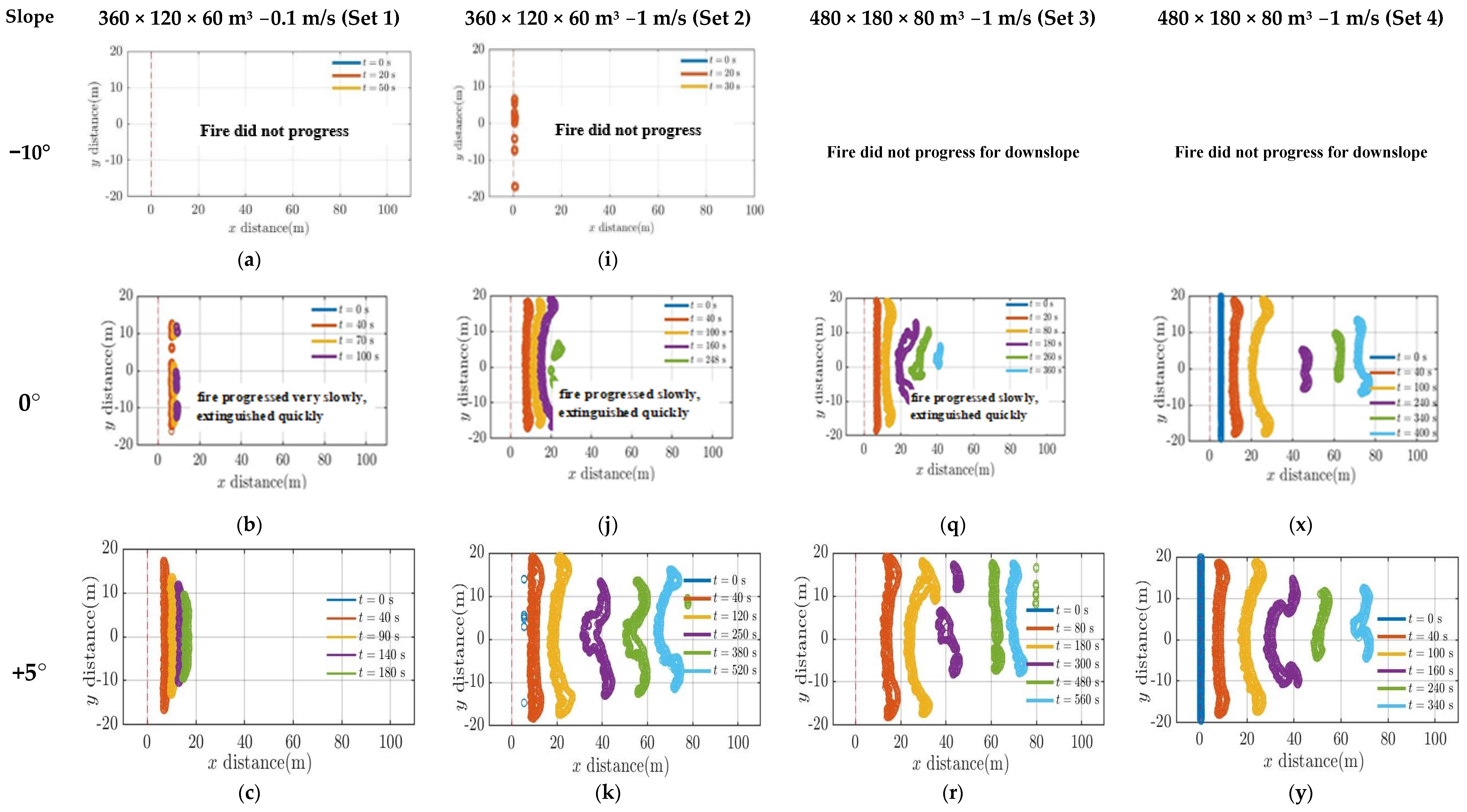
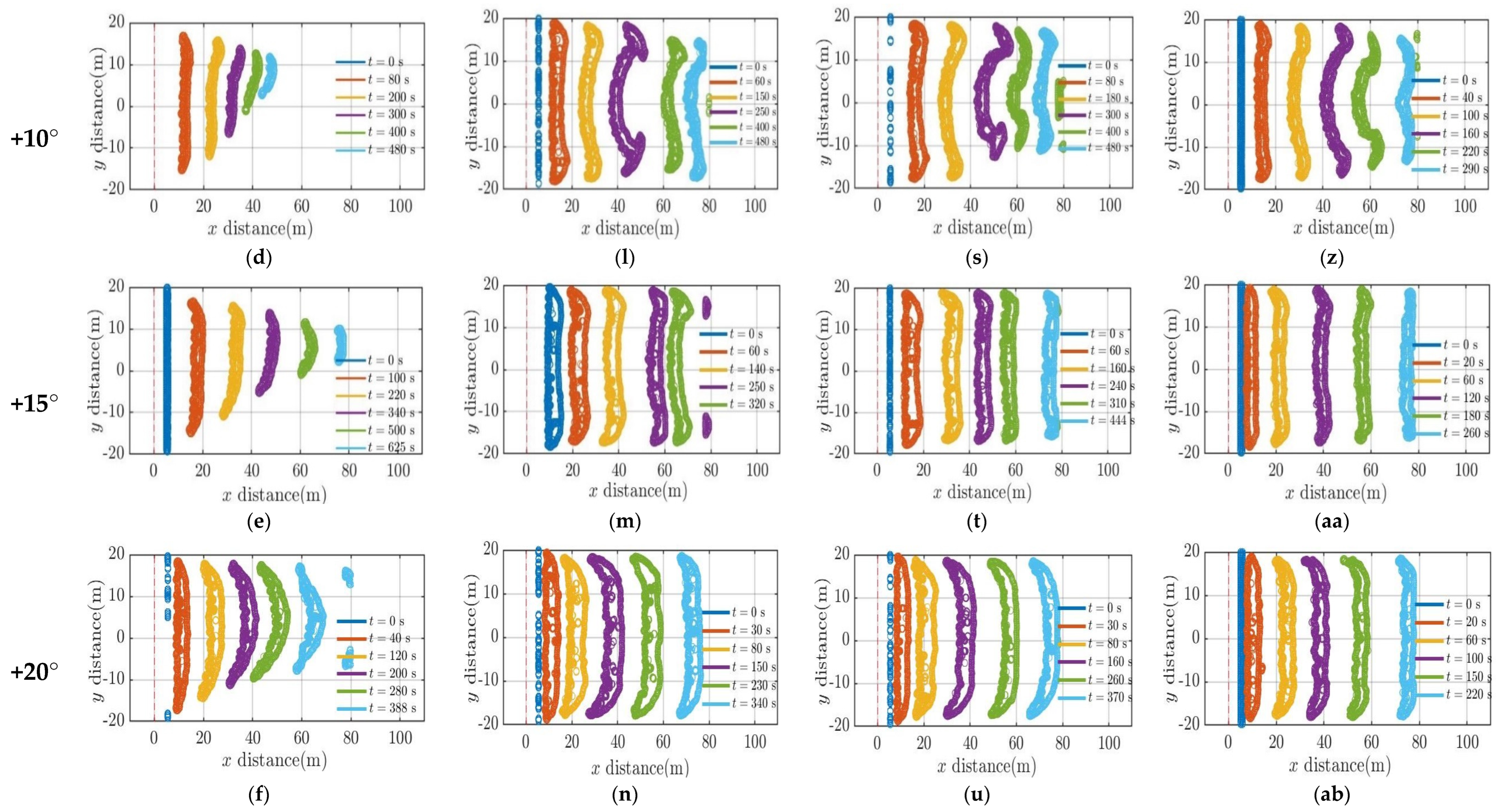
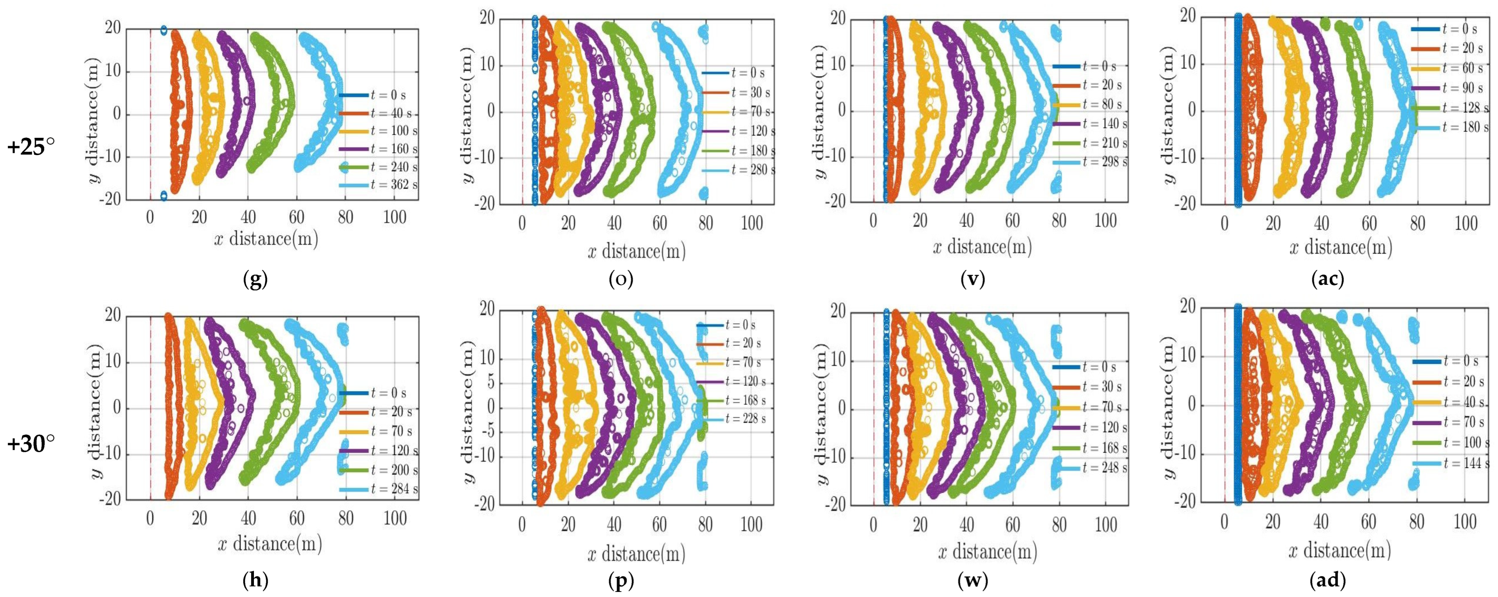
Isochrones sketch out fire’s evolution (the instantaneous leading and trailing boundaries of fire front), as it progresses though the grass plot. These are plotted at different times after ignition in Figure 2. It can be observed that the fire isochrones did not progress for downslope –10°. As observed with downslopes at 3 m/s [1], these lower wind velocities may not be sufficient to drive the fire front as it moves downslope, and the fire is extinguished instantly. Hence, steeper downslopes are not simulated, and downslopes are not discussed further in this paper. Again, for 0° and lower upslopes (0°, +5° at 0.1 m/s and 0° at 1 m/s), the fire isochrones progressed very slowly and extinguished much earlier as evident in the frames (Figure 2a,b,h,o).
As the slope angle increases, the pyrolysis width expands and reaches the end of the burnable grass plot earlier. Notably, for the same slope angle, an uptick in wind velocity accelerates the pyrolysis front, enabling it to traverse the grass plot at a faster pace. This observation is aligned with findings from the higher velocity scenarios discussed in [1], which highlighted that the pyrolysis front travels more quickly with an increase in wind velocity and slope angle.
At gentler slope angles, fire isochrones show an inward shape pattern (up to +10° for 0.1 m/s and up to +15° for 1 m/s cases) rather than assuming a typical convex shape. This could be attributed to the formation of vortices at the fire’s extremities, promoting faster propagation at the edges than at the central region. In higher wind cases [1], the driving wind dominates moulding the fire into the typically expected parabolic shape. Understanding the different shapes of fire line curvature can be a potential topic for future studies. As the slope angle increases (in some cases as the isochrones travel downstream), the contours evolve into a more pointed convex curve that is sharper at higher upslopes. This agrees with the experimental studies conducted by Dupuy et al. [38] with no wind. They observed that on +20° and +30° upslope fires, the fire isochrones changed to a pointed V-shape, in contrast to the smoother curvatures seen on flat terrains. While our simulation settings (the geometry, boundary conditions, length of the fuel bed, and fuel type) differed from those of Dupuy et al. [38], it is evident (in Figure 2) that fire contours tend to become sharper with increased upslope. Furthermore, the fire isochrone patterns generally concur with the experimental observation of Tihay et al. [39], who noted a V-shaped pattern in a +20° slope fuel bed in no-wind conditions.
Comparing the domain sizes (Set 2 and Set 3), we did not observe any notable variations in fire isochrone patterns. Again, comparing Set 3 and 4 simulations, which had varied fuel parameters, the fire isochrones generally demonstrated similar progression patterns. However, we noted longer fire propagation for lower slope angles (0° and +5°) with “lighter & drier” fuel (Set 4). Again, Set 4 shows slightly more convex curvatures and a thinner pyrolysis width.
Pyrolysis width can be indicative of fire line intensity, making its analysis useful for operational modelling. Figure S1 of the supplementary document (Annexure A) charts the pyrolysis width over time for all simulation sets. Generally, the pyrolysis width increases as the fire front progresses from the ignition line, then plateaus or reaches a quasi-steady state and finally decreases. However, for high upslopes (+25° and +30°), the values fluctuate, and the plateau is observed only for a short period of time. Generally, as the upslope angle increases, the width of the plateau decreases, and its magnitude or value increases. The pyrolysis widths for +5° and +10° are lower compared to other slope cases, consistent with Figure 2, where the isochrones are moving very slowly at lower slope angles and the fire is extinguished relatively quickly.
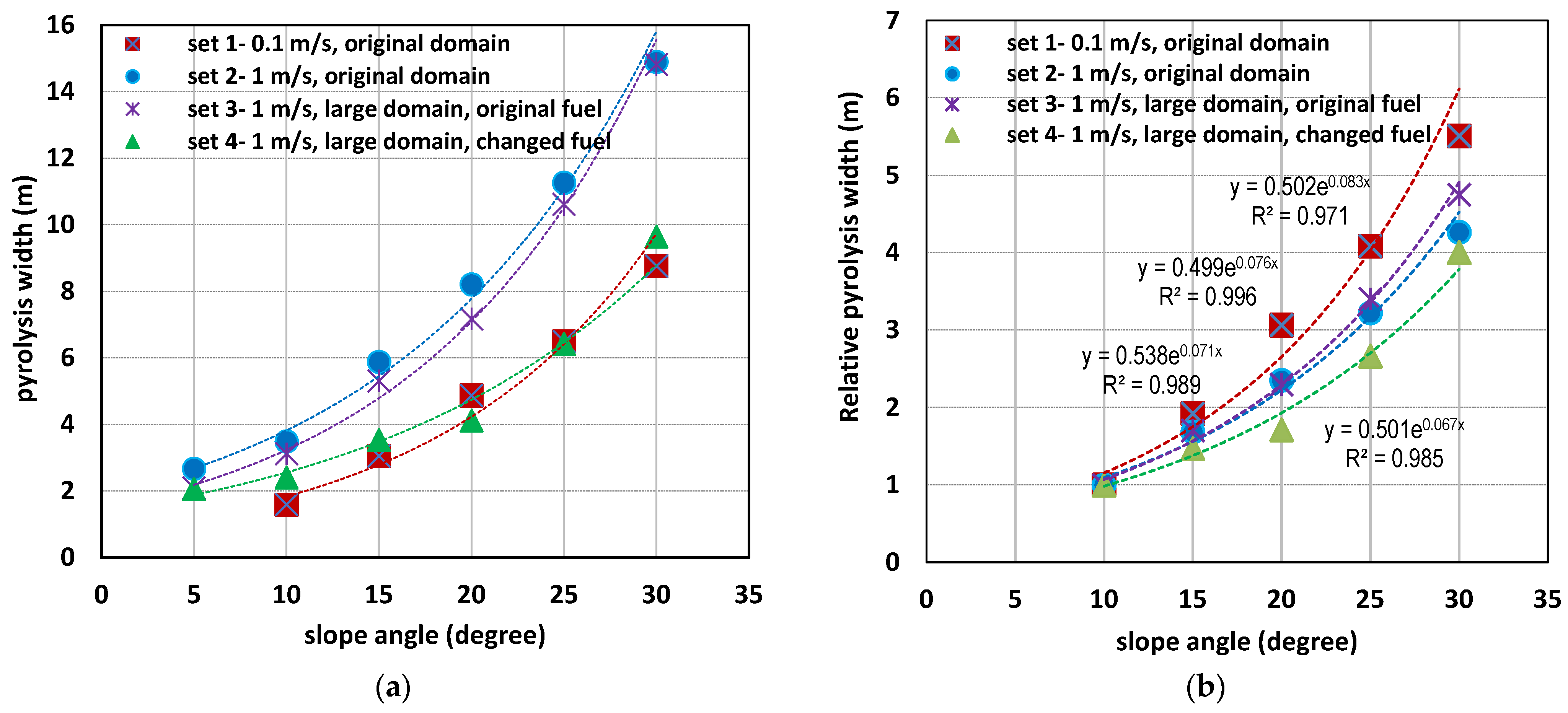
Figure 3a shows the quasi-steady pyrolysis width vs slope angle for across all simulation sets. The quasi-steady pyrolysis width values are extracted within an approximate range of 40 to 200 s post-ignition for Sets 1, 2, and 3 and 20 to 120 s for Set 4. Notably, for +25° and +30° slopes, pyrolysis width values are approximate as the fire front reaches the end of the burnable grass plot more quickly, attaining peak values much earlier. Lower slope angles consistently displayed reduced pyrolysis width values, with Set 2 showing a considerable decrease of around 75% when transitioning from a +10° to a +30° slope.
The relationship between pyrolysis width and slope angle can be constructed as a linear, exponential, or second-order polynomial for all four sets of simulations. The coefficient of determination R2 exceeds 0.95 for all these relationships with the exception in linear relationship for Set 4, where R2 = 0.88. Generally, the pyrolysis width was found to approximately double at every +10° increase in upslope, across all four sets, suggesting an exponential trend. It is to be noted that doubling of RoS at every +10° increase in slope is considered as a rule of thumb for Australian empirical models. Therefore, in Figure 3a, only exponential trend lines are displayed.
Comparing the pyrolysis width of the two domain sizes (Sets 2 and 3)—both having identical driving wind velocities and fuel characteristics—the values remain closely aligned across all slope angles. The expanded domain size has insignificant effect on pyrolysis width, mirroring the similar fire isochrones pattern observed in Figure 2 for Sets 2 and 3. The pyrolysis width with changed fuel (comparing Sets 3 and 4), with the same driving wind velocity and domain size, reveals fuel characteristics’ significant influence on pyrolysis width. Pyrolysis width is consistently narrower with “lighter & drier” fuel parameters across all slope angles. As anticipated, elevated ambient temperature combined with reduced relative humidity of air, fuel moisture content, and fuel load contribute to this reduction.
We then obtained the relative pyrolysis width for each scenario by normalizing the actual pyrolysis width against the pyrolysis width of the scenario with a +10° slope within the same set. Since the fire did not progress for lower slope angles (0° and +5° at 0.1 m/s and 0° at 1 m/s), a +10° slope is chosen as the base to determine the relative pyrolysis width instead of a 0° slope. The relative pyrolysis width vs slope angle profiles are plotted in Figure 3b. Much like the pattern observed with quasi-steady pyrolysis width vs slope angle, an exponential relationship (R2 value shown in the figure) can be constructed between relative pyrolysis width and slope angle. The value of the coefficient is ~0.5 for all four curves and the exponent lies between 0.067 and 0.083. A stronger slope effect is observed for 0.1 m/s wind velocity cases (Set 1) compared with 1 m/s cases (Sets 2, 3, and 4) and the difference widens as the slope angle increases. This may be associated with longer residence times with the slower velocity. Generally, the pyrolysis width effect is found to be identical for 1 m/s wind velocity cases (Sets 2 and 3).
It is often considered that pyrolysis width is a reflection of fire size or fire intensity. In the following subsection, we attempt to establish a relationship between pyrolysis width and fire intensity.

4.2. Heat Release Rate (HRR) and Fire Intensity

The time series of HRR obtained from all four simulation sets of simulations are presented in Figure S2 of Annexure A.
Byram’s fire intensity [23] Q (kW/m) is calculated by dividing the HRR values (kW) by the fireline length (m). The instantaneous fireline length, running across the width of the fire isochrone plots (isochrones shown in Figure 2), is measured every 20 s following the method demonstrated in Figure 9 of [1]. As for no slope and lower upslope angles, the fire eventually extinguished at these lower wind velocities; it was not possible to measure meaningful fire front lengths (Figure 2). Hence, 0°, +5°, and +10° at 0.1 m/s and 0°, +5° at 1 m/s are not included in the fire intensity (Q) plots in Figure 4. Again, at the lower upslope angle +10°, the fire isochrones did not attain a convex curvature, and hence, the measured fire front lengths for +10° for the four sets are approximate. Q values as a function of time are presented in Figure S3 of Annexure A for all sets of simulations. The HRR and Q generally increase upon ignition, then decrease for a while and surge again. Once the ignition source is removed, the fire intensity starts decreasing. However, with increased pyrolysis, the intensity starts to increase again. For all four sets, the HRR (and hence Q) increases with slope angle, attains a peak value, and then reaches a quasi-steady state.
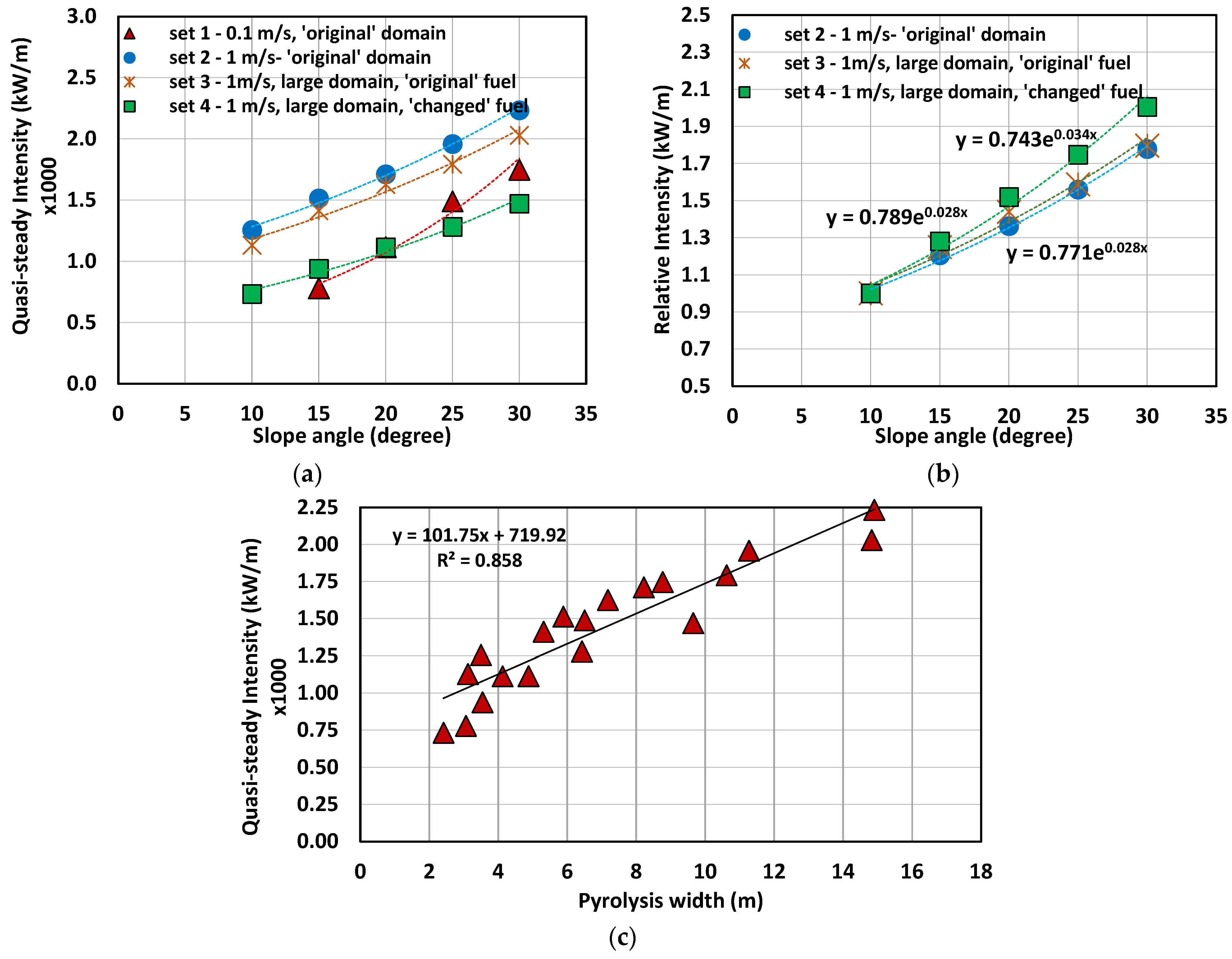
The averaged Q values extracted from the quasi-steady region are plotted in Figure 4a. The Q value increases with the driving wind velocity and slope angle when the fuel characteristics are the same. For 1 m/s cases (Sets 2, 3, and 4), the quasi-steady Q values increase by approximately 30–50% at every +10° increase in slope, whereas the increase is approximately 60–90% for 0.1 m/s cases.
Upon comparing the Q values between the two domain sizes (Sets 2 and 3), no significant difference is observed across all slope angles, mirroring the observation with pyrolysis width (Figure 3a). When comparing Sets 3 and 4, the Q values decrease with the “lighter & drier” fuel characteristics as also reflected in the pyrolysis width (Figure 3a).
The relationship between Q and slope angle can be constructed as a linear, exponential or second-order polynomial, as we observed for the pyrolysis width results. For all three types of relationships, the R2 value exceeds 0.97, indicating a strong fit. Given the negligible difference observed in the R2 values among these relationships, an exponential relationship is deemed to represent the correlation between Q and slope angle, akin to that with pyrolysis width, as reasoned in Section 4.1. The exponential trend lines (for visual representation only) are shown in Figure 4a.
Figure 4b shows the relative intensity (quasi-steady intensity on any slope divided by quasi-steady intensity at +10° slope) vs slope angle only for 1 m/s cases. A slightly stronger effect of slope on the relative intensity is observed for the “lighter & drier” fuel. Generally, the values of the coefficient and exponents are ~0.75 and ~0.03, respectively. We observe a much smaller exponent for the relative intensity compared to the relative pyrolysis width.
The quasi-steady intensity vs pyrolysis width is plotted in Figure 4c. Constructing a linear relationship through the least square approximation method, an R2 value of approximately 0.86 is observed. Alternatively, a logarithmic relationship can be formed, yielding an R2 value of around 0.89. However, given the uncertainties inherent in simulations, it is reasonable to assert that these two parameters are linearly correlated.

4.3. Fire Front Locations, Dynamic RoS, and RoS Calculations

This section discusses the RoS calculations and their correlation with slope angles. The RoS values obtained from WFDS simulations are then compared with the results from various empirical models: McArthur MK III and MK V, CSIRO, and Rothermel “Original” and “Modified” models. Subsequently, relative RoS (defined as the RoS on any slope divided by RoS at a reference slope) from WFDS are compared with the Australian slope function (rule of thumb) and the Rothermel model variations.

4.3.1. Fire Front Locations

Figure 5a,b depict the fire front location for Set 1 and 2 simulations, respectively. Figure 5c shows fire front locations for Set 2 and 3 simulations in a single plot, comparing the original and large domain sizes while conserving the same driving wind velocity (1 m/s) and fuel characteristics. In Figure 5d, fire front locations for Sets 3 and 4 (original and “lighter & drier” fuel, respectively), while preserving the same driving wind velocity (1 m/s) and domain size, are presented to demonstrate the effect of fuel characteristics on fire front propagation. Continuous lines represent the fire front locations with the original domain size and original fuel parameters and the dashed lines represent those of the larger domain and changed (“lighter & drier”) fuel parameters.
As anticipated, the fire front advances faster with a steeper slope. With the reduction in wind velocity, the fire front travels more slowly, consistent with observation from the higher wind velocity cases [1], as corroborated by fire isochrones in Figure 2. Upon comparing the different domain sizes (Figure 5c), for +15° and +20°, the fire front location with the original domain is found to be slightly ahead (by about 2–4 m) of the larger domain, at approximately 100 s post-ignition. Generally, irrespective of domain size, the fire front location remains nearly identical at any given time for a specific slope angle. As echoed in the pyrolysis width findings (Figure 3), enlarging domain sizes exert minimal impact on the fire front locations.
Examining the effect of the fuel characteristics (Figure 5d), at any given time, the fire front travels faster with the “lighter & drier” fuel (lower density, fuel moisture content, and fuel load) and the difference widens as the fire front progresses through the grass plot. Shortly after ignition (around 50–100 s), the fire front location with “lighter & drier” fuel is farther by approximately 30–45% compared to the original fuel.

4.3.2. Dynamic RoS

Following the methodology detailed in Section 3, the rate of spread data are obtained as a function of time with frequency at every second. Dynamic RoS values obtained from the current study are plotted in Figure S4a–d in Annexure A for all simulation sets. The plots show spikes (random fluctuations) in RoS values as the fire front moves on, and the maximum values are observed with +30°.

4.3.3. Averaged RoS

Utilizing the analysis technique applied to higher wind velocity cases [1] (as outlined in Section 3), averaged RoS values are calculated for all scenarios. Figure S5 of the supplementary document presents averaged RoS (both quasi-steady and dynamic-averaged) as a function of slopes, accompanied by whiskers (indicating the upper and lower bounds of dynamic RoS values, serving as a method to display uncertainty in the averaged RoS values). The empirically derived RoS values from different operational models (MK III and MK V, CSIRO, Rothermel Original, and Rothermel Modified models) are also presented in Figure S5a–c as well as in Figure 6 below alongside the RoS values obtained from this study’s WFDS simulations.
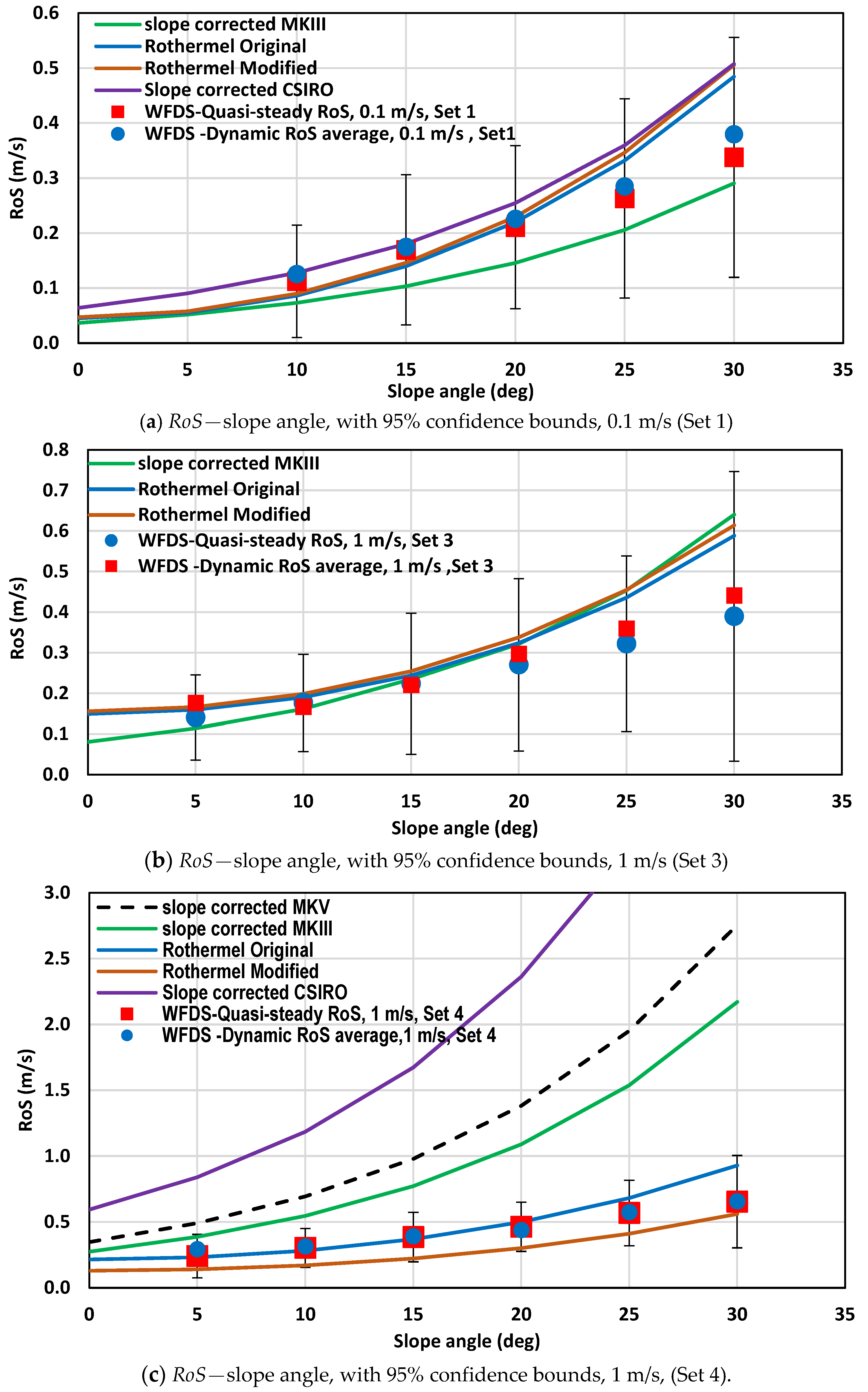
Adhering to the methodology detailed in Section 3.1, uncertainty estimates are calculated and represented as error bars in Figure 6. The length of each error bar around the data point signifies the confidence bounds surrounding the quasi-steady RoSs. Referring to Figure S5a in the supplementary document, the significantly higher MK V values are not shown in Figure 6a and both the MK V and CSIRO values are not shown in Figure 6b.
Figure 6a shows that the quasi-steady and dynamic averaged RoS values obtained from this study are close (with some differences) to slope-corrected MK III and CSIRO model values as well as both Rothermel (Original and Modified) values. The difference ranges from ±0.04 m/s (at +10°) to ±0.17 m/s (at +30°).
Figure 6b for 1 m/s shows that this study’s quasi-steady and dynamic averaged RoS values are quite aligned to slope-corrected MK III and both Rothermel values for slope angles up to +25°, and slightly lower for +30°. However, the CSIRO model values were higher across all slope angles and quite close to dynamic maximum values (as shown in Figure S5b in the supplementary document).
Figure 6c for 1 m/s with changed (“lighter & drier”) fuel parameters reveals that the quasi-steady and dynamic averaged RoS values obtained from this study are closer to the Rothermel Original values for all slope angles up to +25° (slightly lower for +30°) and slightly higher than the Modified Rothermel values for all slope angles.
Both the Original and Modified Rothermel model values align more closely to the quasi-steady and dynamic average RoS values for both lower driving wind velocities. Alongside the findings in [1], this reaffirms that under strong wind influence, Rothermel models exhibit minimal slope effect, and as the wind velocity diminishes, a greater slope effect is observed.
Figure 6a,b, with original fuel parameters, show that the error bar (representing 95% confidence interval) encapsulates all the presented empirical model values for all slopes: CSIRO, MK III, and both the Rothermel model values for 0.1 m/s, and MK III and both the Rothermel model values for 1 m/s. Figure 6c for 1 m/s cases, with “lighter & drier” fuel parameters, shows that both the Rothermel model values are within the error bar range for all slope angles. MK V and CSIRO model values fall outside the error bar range for all slope cases while the MK III model value only for +5° slope is within the range.
Generally, for “original” fuel parameters, the error bar fitted on the WFDS quasi-steady RoS data envelop most of the presented slope-corrected empirical model values. For “lighter & drier” fuel parameters, only the Rothermel model values are found within the error bar range.
For both lower wind velocities, the correlation between quasi-steady RoS and slope angles aligns more closely with an exponential relationship (R2 values are shown in the plots, Figure S5 of the supplementary document). As observed in [1], the relationship for 3 m/s scenarios can also be developed as exponential. This implies that the RoS vs slope angle relationship transitions to an exponential fit at lower wind velocities. It is plausible that as the driving wind velocity decreases, the relationship morphs into an exponential one, resonating with the exponential correlation reported in most of the experimental studies conducted with negligible or very low wind speeds [14,40,41]. The exponential relationship between RoS and slope angle are summarized in Table 3.
Australian practitioners often use a “rule-of-thumb” stating that the RoS of fire doubles for every 10° upslope increase or halves with every 10° increase in negative slope ([6,42]). Table 4 shows the RoS (WFDS quasi-steady) percentage changes at every +10° slope (derived from Figure S5) for this study’s simulations.
Within the confines of this study’s simulations, for 0.1 m/s wind velocity, the quasi-steady RoS values increase by 55% to 87% for every 10° increase in upslope. For 1 m/s (both Sets 3 and 4), the range is ~45–60%. Generally, it is observed that the difference in RoS values for every 10° increase upslope narrows as the slope angle increases. The fire isochrones did not progress for downslopes at the lower wind velocities, and therefore it is not possible to comment on the negative slope scenario at very low wind speed.

4.3.4. Relative

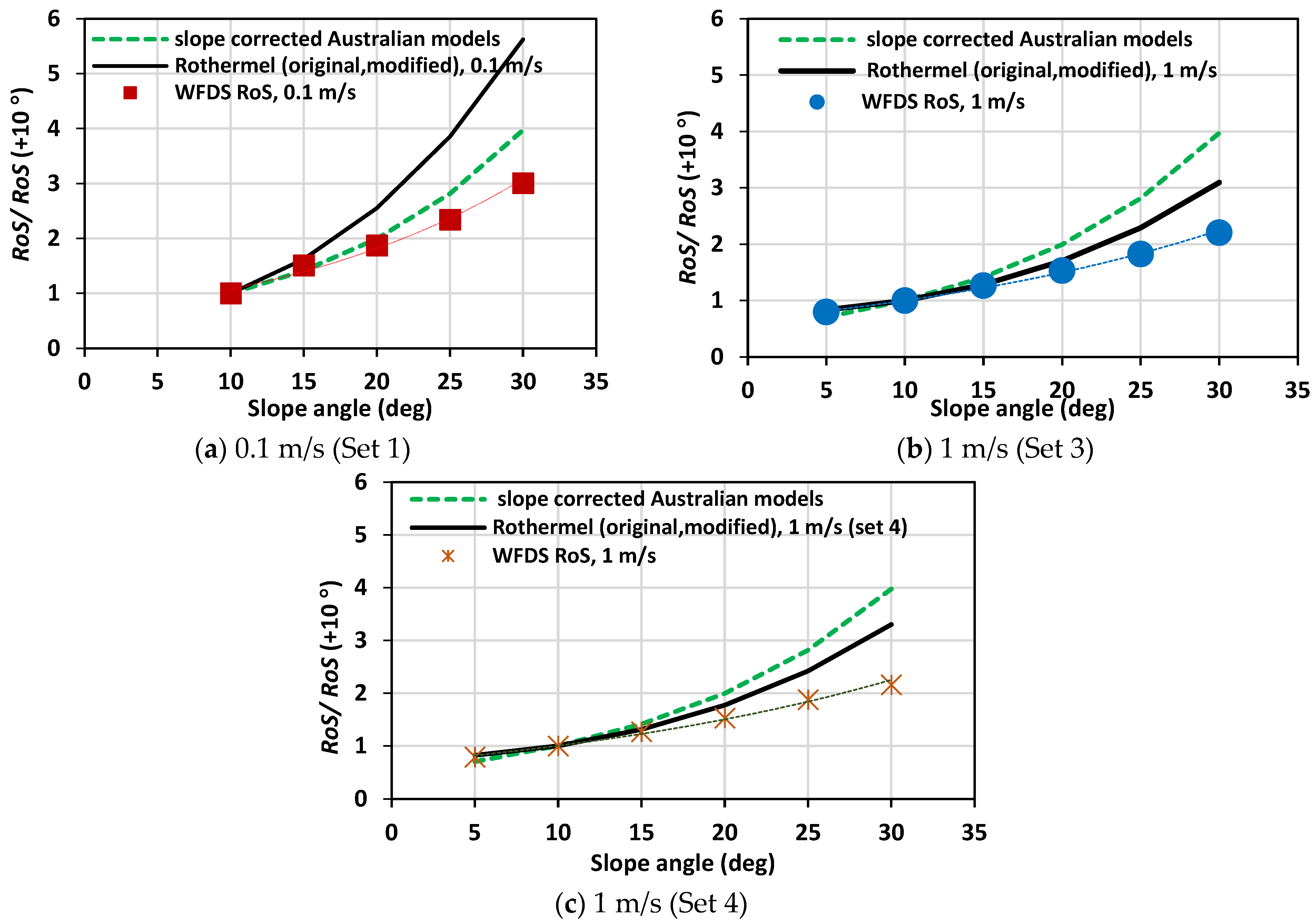
Figure 7 presents the relative RoS (RoS on any slope divided by RoS at +10°) from WFDS modelling (from Figure 6) compared with the Australian slope function (rule of thumb) and Rothermel model variations. Since the fire front did not progress at lower slope angles (0° and +5°) for some sets, and did not reach steady state conditions, we based the relative RoS on a +10° slope as the reference rather than the 0° slope.
In the context of higher wind velocities discussed in [1], the relative RoS remains constant for the Australian model slope function. Australian models MK III, MK V, and CSIRO models consistently produce identical relative RoS values across all sets due to their inherent multiplicative nature. Both the Original and Modified Rothermel models produce consistent values for each wind speed, whereas WFDS-relative RoS results return separate values.
Interestingly, the Rothermel model exhibits a pronounced slope effect at these lower wind velocities. This contrasts with the results obtained for higher wind velocity cases [1], where the Rothermel model showed minimal slope influence. The Australian models’ slope function under low or near-zero wind velocities (Figure 7a) aligns more closely with the WFDS quasi-steady results than it does at higher wind velocities (see Figure S6 in the supplementary document) [1]. For the 1 m/s wind velocity (Figure 7b), the Rothermel model’s relative RoS is closer to WFDS values than the Australian models. The relative RoS follows the same trend for both the original and “lighter & drier” fuel characteristics, as demonstrated in Figure 7b,c.
Mendes-Lopes et al. [43] deduced from their experiments that the strongest influence on RoS is by far wind velocity, followed by fuel moisture content, then slope. The Rothermel model results corroborate this, emphasizing wind’s stronger influence than slope on RoS. In general, our WFDS-relative RoS result sat the lower driving wind velocities of 0.1 and 1 m/s, nearer to the relative RoS functions predicted by the empirical slope corrections of Australian and Rothermel models.
The relationship between WFDS-relative RoS and slope angle can be construed as both a second-order polynomial and exponential function, as shown in Table 5, with R2 > 0.99 for both functions at both wind velocities. The trend lines for the exponential relationship (as the Australian slope correction is exponential) between relative RoS and slope are shown in Figure 7.

4.3.5. Fire Intensity Q as a Function of RoS

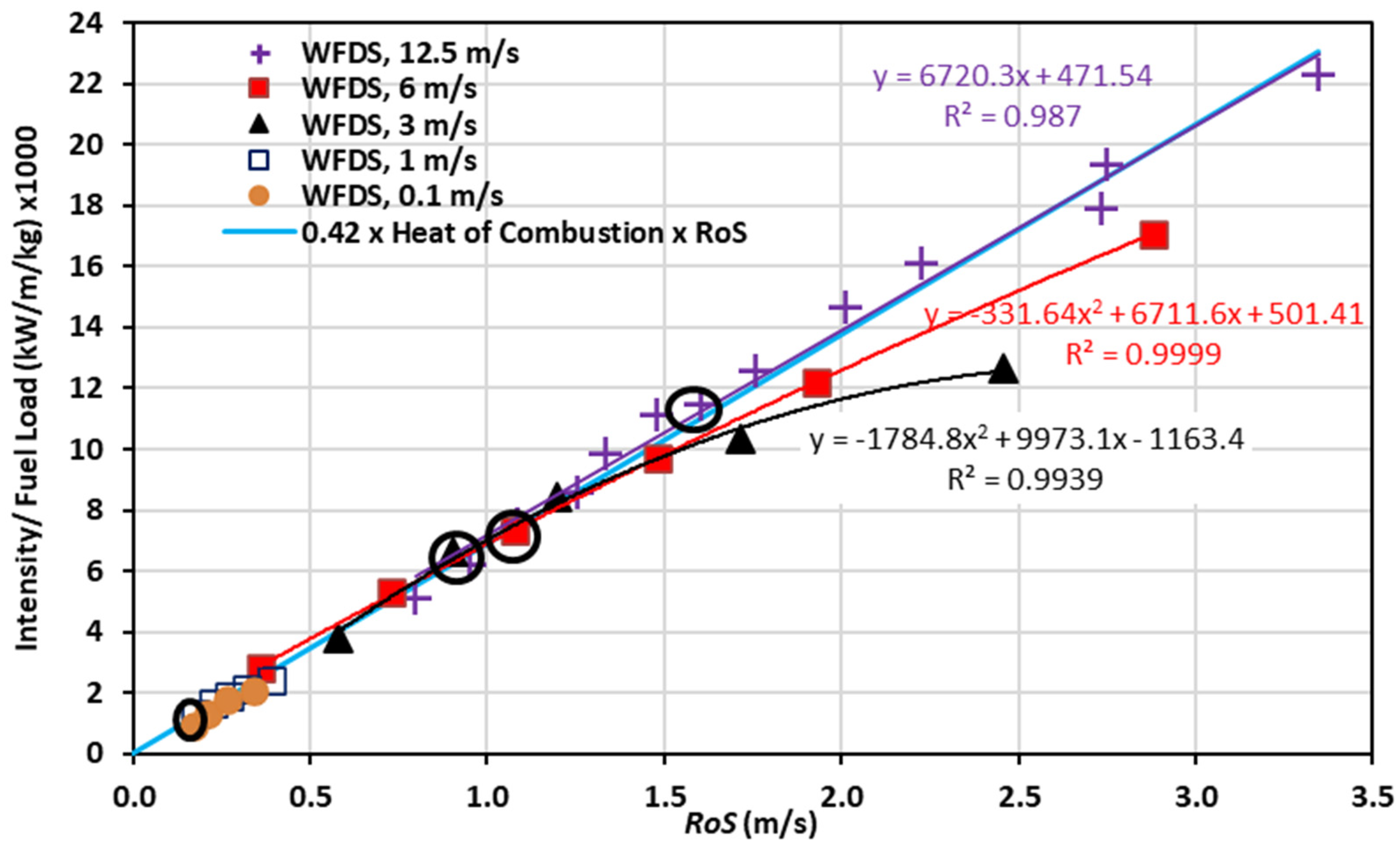
In Figure 8, the Q values obtained for all five wind velocities (0.1, 1, 3, 6, and 12.5 m/s) are normalised with the respective fuel loads and plotted against the corresponding RoS values. The fuel load for higher wind velocities of 3, 6, and 12.5 m/s was 0.283 kg/m2 [1], while the load for the lower wind velocities of 0.1 and 1 m/s (Sets 1 and 3) in this study is 0.85 kg/m2 (Table 2). Black circles in the plot denote values at no-slope cases for all wind velocities. As stated in Section 3.1, the fire front did not progress for 0°, +5°, and +10° at 0.1 m/s and 0°, +5° at 1 m/s and hence the related data were not included in the analysis.
In Figure 8, when data points across five velocities are considered, a linear correlation emerges, suggesting a linear relationship governed by the formula, Q/fuel load = 0.42 × heat of combustion × RoS for all cases, except upslopes ≥+20° at 6 and 3 m/s wind velocities. Therefore, in general, with ~42% fuel consumption, Byram’s intensity (Equation (7)) can be—Q = 0.42 × fuel load × heat of combustion × RoS—satisfied.

4.4. Plume and Flame Dynamics at Lower Wind Velocities

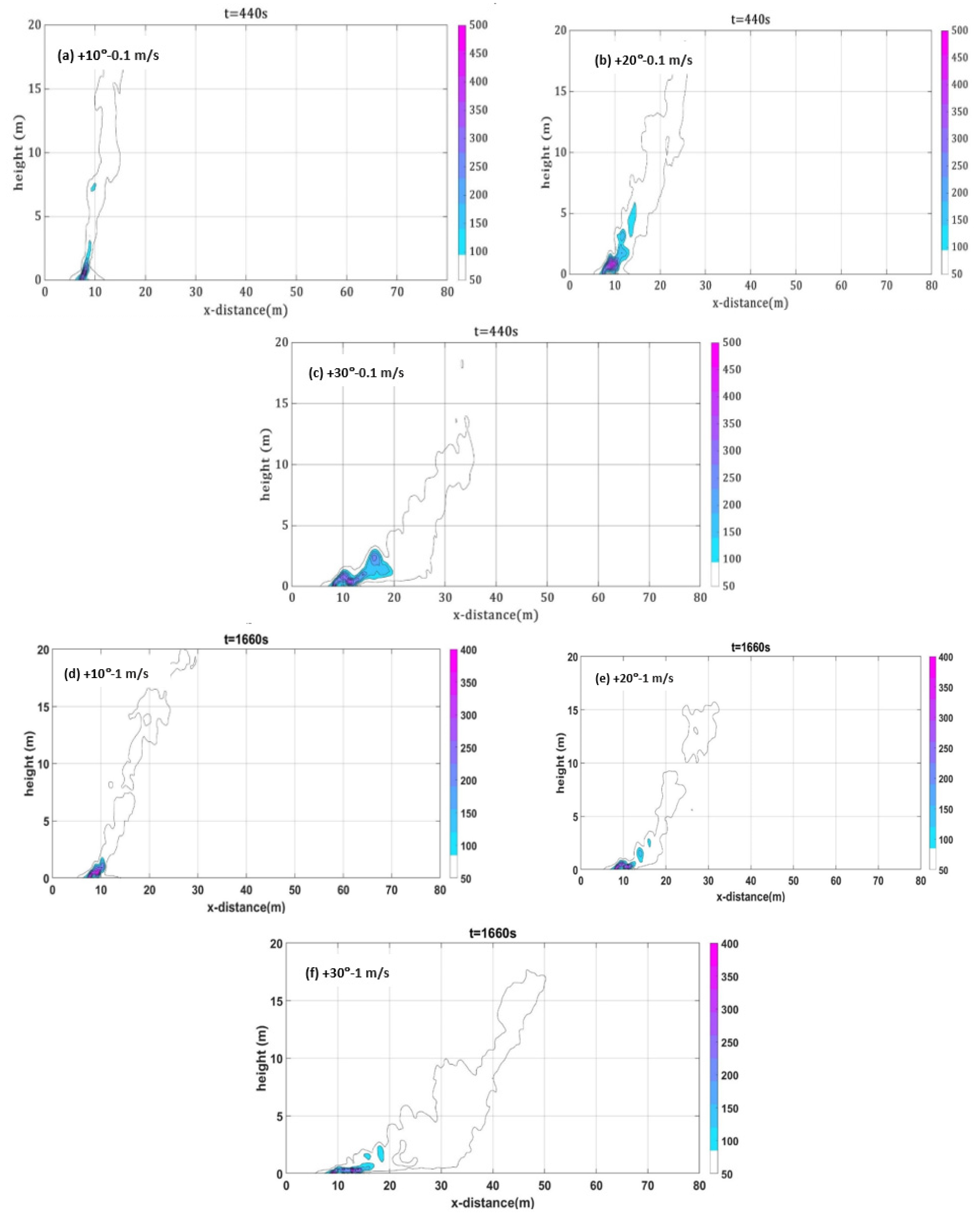
Figure 9 captures the temperature contours, representing plumes, for each slope case at the same time (40 s after ignition) as the fire advances though the burnable grass plot in the x-direction. The plume’s colour shading represents air temperature (in K, indicated in the colour bar). These plots provide a snapshot of the plume’s behaviour at that specific moment revealing whether it is attached to the ground or up-rising.
Plumes (instantaneous) emanating from the fire front for +10°, +20°, and +30° at wind velocity 0.1 m/s are shown in Figure 9a–c and at 1 m/s are shown in Figure 9d–f. For both low wind velocities, the plume rises from the ground near the ignition line for +10° slope, and for higher upslopes, the buoyant plume leans towards the ground for a longer distance. As the slope angle decreases, the plume detachment occurs closer to the ignition line. The plume is leaned more towards the ground at +30° (Figure 9c,f) compared with lower slope angles.
Previous studies [2] indicated that even on a −10° slope with 12.5 m/s wind, the plume is leaned (leading to its attachment) to the ground, whereas on the same slope with 3 m/s, the plume is only partially attached to the ground, and it is generally rising. This suggests that higher wind leads to inclination even on downslopes. Like Dold and Zinoviev [44] and Sharples [6], we observe in Figure 9a–c that with almost no wind, steeper slopes cause greater plume inclinations.
Combining higher wind and higher velocity, one expects a more pronounced inclination of the plume toward the ground. However, no significant eruption is detected in our simulations. For a given slope angle, the plume rises from the ground earlier at 0.1 m/s than at 1 m/s, though a minimal difference is observed. Generally, a distinct detached or rising plume is evident for upslopes at both wind velocities. When compared with the higher wind velocities presented in [2], for any given slope angle, the plume rises much sooner from the ignition line.
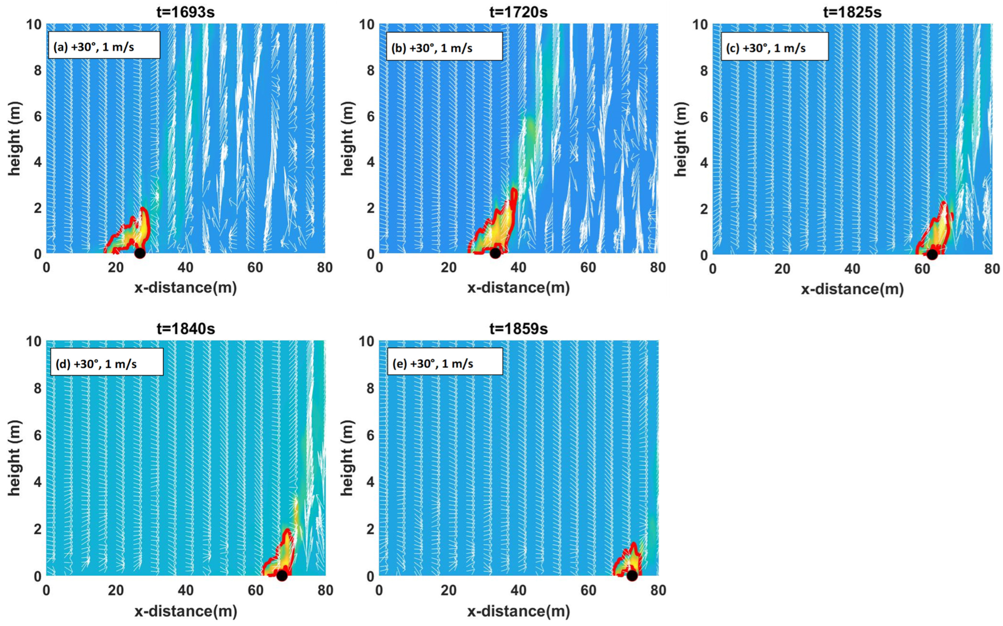
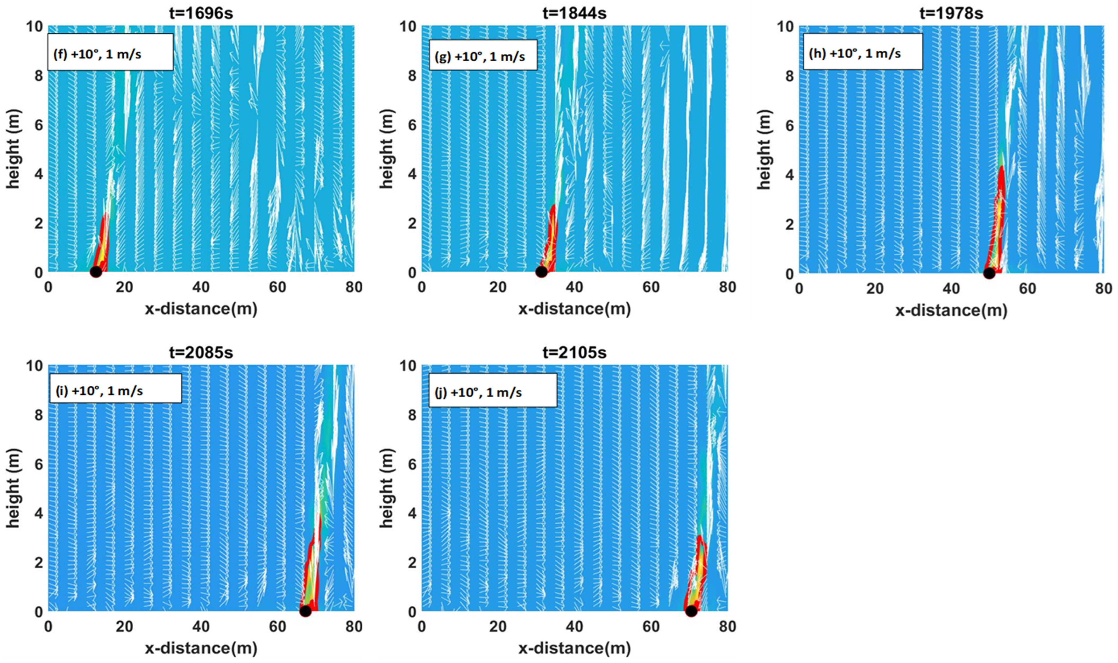
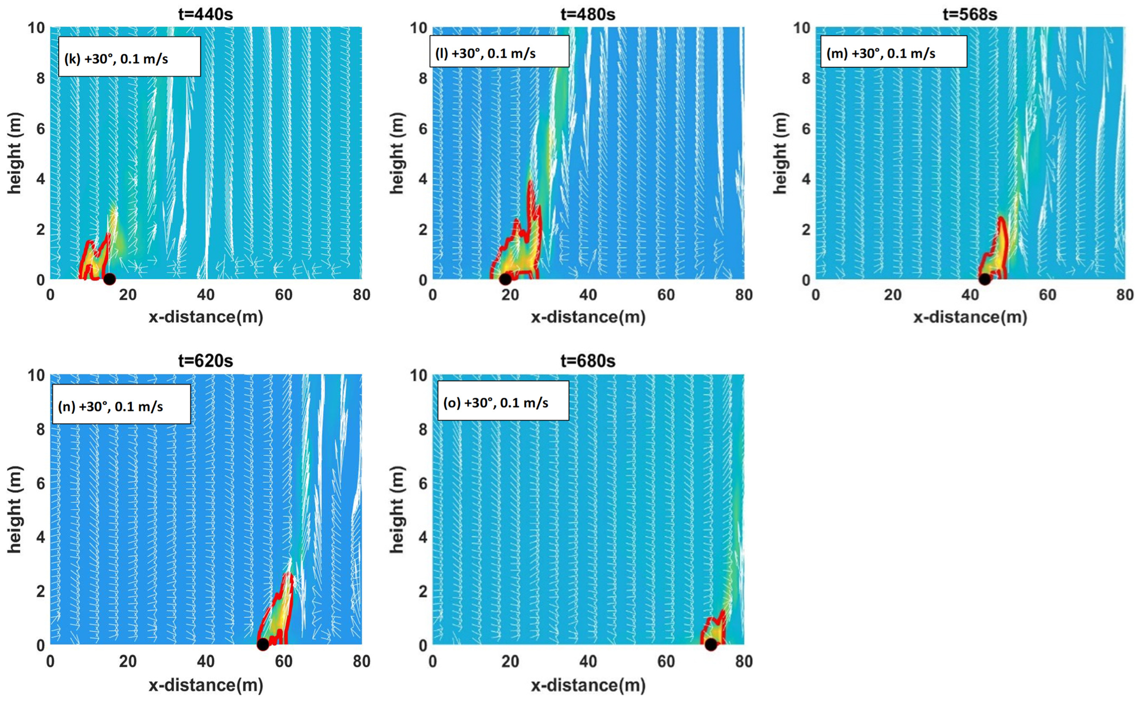
The flame contours, temperature contours, detachment location, and velocity vectors are visualized in Figure 10 to understand flame behaviour. Streamwise and vertical components of wind velocity U and W, HRR and temperature data taken through the centreline of the burnable grass plot, are used to obtain the velocity quiver plots along with flame and temperature contours. As for higher wind velocity cases [2], the flame envelopes are determined from the minimum threshold temperature of 400 K to the maximum temperature of the flame.
Figure 10 shows flame contours (red) with temperature contours shaded in the background (yellow) along with detachment locations (black dots) and wind vectors (white arrows) for both the wind velocities (Sets 1 and 3) at slope angles +30° and +10°. The detachment location shown in these frames is where the plume lifts off from the ground at that time frame. Figure S7 in the supplementary document shows these contours for +20° slope at 0.1 and 1 m/s. Comparing Sets 2 and 3, like other parameters, we noticed minimal variation in flame contour patterns, leading us to exclude Set 2 from Figure 10.
For a wind velocity of 1 m/s at the steepest slope angle, +30° (Figure 10a–e), the near-flame is vertical, and the flame-perturbed velocity vector is inclined upward. A buoyancy-dominated flame is observed as the fire progresses. The fire establishes itself and then becomes attached for a very short time, which leads to rapid intensification and a buoyancy-dominated fire. The plumes (represented by temperature contours) emanating from the grass plot are also rising (and vertical). This is consistent with the graphical representation of the plume plotted in Figure 9d–f. With lower slope angles, the flame points more directly upwards (is more vertical) and is taller compared with the higher slope angles, as evident in Figure 10f–j. The flame is more vertical at +10° compared with that for steeper upslopes. For +30°, the flame appears to be attached for a very short period earlier in the fire progression (two-sided wind entertainment can be seen into the plume, but not into the flaming zone), prior to rising.
The 0.1 m/s plots generally mirror the 1 m/s trend; flames are clearly vertical (rising) and for lower slope angles, the flame is more vertical but becomes wider at the steepest slope +30°. However, for a given slope angle, the flame is wider for 1 m/s cases compared with 0.1 m/s. With 0.1 m/s, the plume emanating from the grass plot also rises vertically, consistent with the graphical representation of the plume plotted in Figure 9a–c. Flame detachment is more pronounced in the +10° cases at 0.1 m/s (shown in Figure 10p–t).
It is evident from the flame and plume contours presented in Figure 10 that, for lower driving wind velocities, the flame dynamics, as well as the plume, appear detached or up-rising. Fire propagation is clearly within the plume or buoyancy-dominated regime. In the following section, Byram number (Nc) analysis is performed to quantify the mode of fire propagation as wind-driven or buoyancy-driven.

4.5. Mode of Fire Propagation

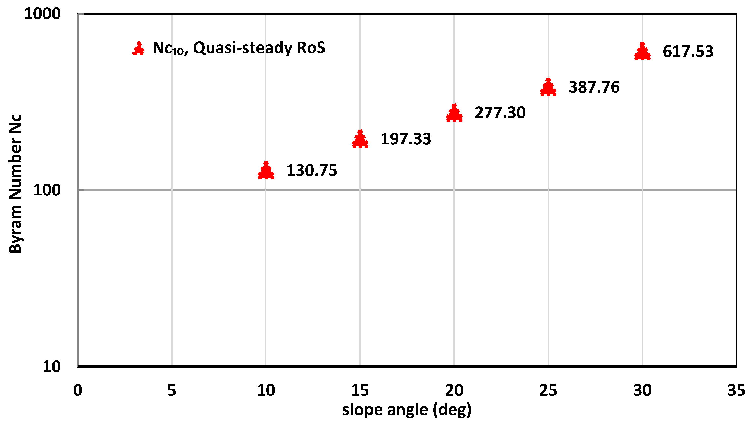
Byram number, Nc, is calculated using Equation (6) [25] for cases with all slope angles, at 1 m/s wind velocity (simulation Set 3). Only results with 1 m/s cases are presented in Figure 11, as meaningful values could not be obtained with 0.1 m/s wind velocity cases (with RoS values higher than U10, the denominator term (U10RoS)3 in Equation (6) gives negative values, resulting in negative Nc values). Different Nc values can be obtained using wind velocity at different reference heights and either dynamic or quasi-steady RoS, but none are significant enough to change the classification of the mode of fire propagation.
It is worth noting that the Nc typically describes forces that are nominally perpendicular. However, wind and slope can incline flame towards the surface. Past studies used Nc for assessing whether fire propagation is wind-driven or plume-driven. Therefore, it is rational to use Nc for slope cases. However, caution needs to be exercised in interpreting the Nc values obtained in this study for steep upslope cases.
Given the large Nc values (Figure 11), all scenarios can be classified as buoyancy-driven, yet we observed attached flames for slope angles ≥ +20°. This agrees with flame and plume contours presented in Figure 9 and Figure 10 that for ≥+20° slopes, the flame and plume were found to be attached to the ground for a short period before transiting into a buoyancy-driven propagation. This indicates that Byram number analysis may not be sufficient to determine the mode of fire behaviour in greater upslopes. In contrast, the higher wind velocity cases presented in [2] demonstrated that, for the highest wind velocity of 12.5 m/s, the flame and near-surface flame appeared to be rising even though the plume was attached. For wind velocities of 12.5 and 6 m/s, the flame was found to be buoyancy-dominated near the ground, tended towards wind-dominated for a very short time, and then transited to a buoyancy-dominated regime as the fire progressed. The flame behaviour was found to be different from the overall plume behaviour [2].

4.6. Flame Length

Figure S8a,b in Annexure A plots flame length over time for wind velocities of 0.1 (Set 1) and 1 m/s (Set 3), respectively. Given the fire’s dynamic nature, flame lengths fluctuate and display irregular patterns. As observed for higher wind velocities, the highest flame length is at +30° slope and the flame length decreases as the slope angle decreases. For 1 m/s wind velocity, the flame length for every +10° increase in slope increases by approximately 40–70%, and for 0.1 m/s, it increases by approximately 64–90%. This observation is consistent with the plume contour view in Figure 9, when increased upslopes lean the plume more towards the ground, making the plume’s attachment likelier. Like pyrolysis width (observed in Figure 3), protracted quasi-steady states are more apparent at gentler slopes.
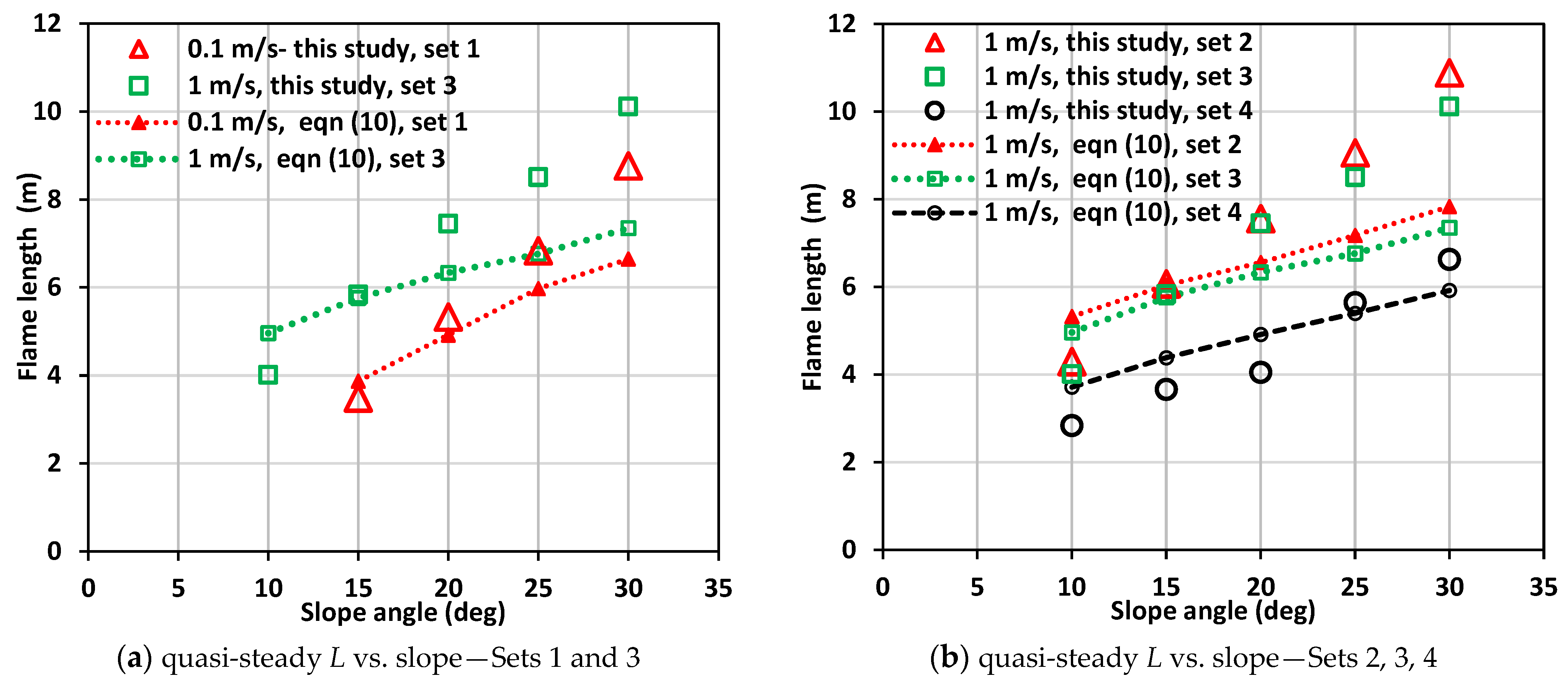
The flame lengths (L) extracted from the quasi-steady region are plotted in Figure 12a,b; for Set 1 and Set 3 in Figure 12a; and for Sets 2, 3, and 4 in Figure 12b. For steeper upslopes, where no clear quasi-steady state exists, the flame length is averaged over a short period at the peak of the length. Comparing the wind velocities (Sets 1 and 3), for a given slope angle, the flame length is generally lower for the lower wind velocity, 0.1 m/s. This mirrors the high velocity findings in [2], which showed the flame length decreased with wind velocity.
Upon comparing flame lengths between two domain sizes (Sets 2 and 3)—with the same driving wind velocity and fuel characteristics—the flame lengths are nearly the same across all slopes. This was also observed for pyrolysis width, fire front, and HRR. Evaluating flame lengths with “lighter & drier” fuel characteristics (comparing Sets 3 and 4) indicates that fuel characteristics significantly influence the flame length. Flames are shorter with changed fuel parameters across all slope angles. As observed in Figure 4, Set 4 simulations produced lower intensity, which resulted in lower flame length. The decreased fuel load is likely the reason for this result.
The corresponding flame lengths derived using Equation (8) are also presented in Figure 12. For the “lighter & drier”, the agreement with WFDS results reasonably well. The agreement is not as good for the original fuel, especially on higher slopes. If modifying the exponent from 0.67 to 0.7 in Equation (8), it yields a better alignment for simulations with the original fuel and slopes ≥+20°.
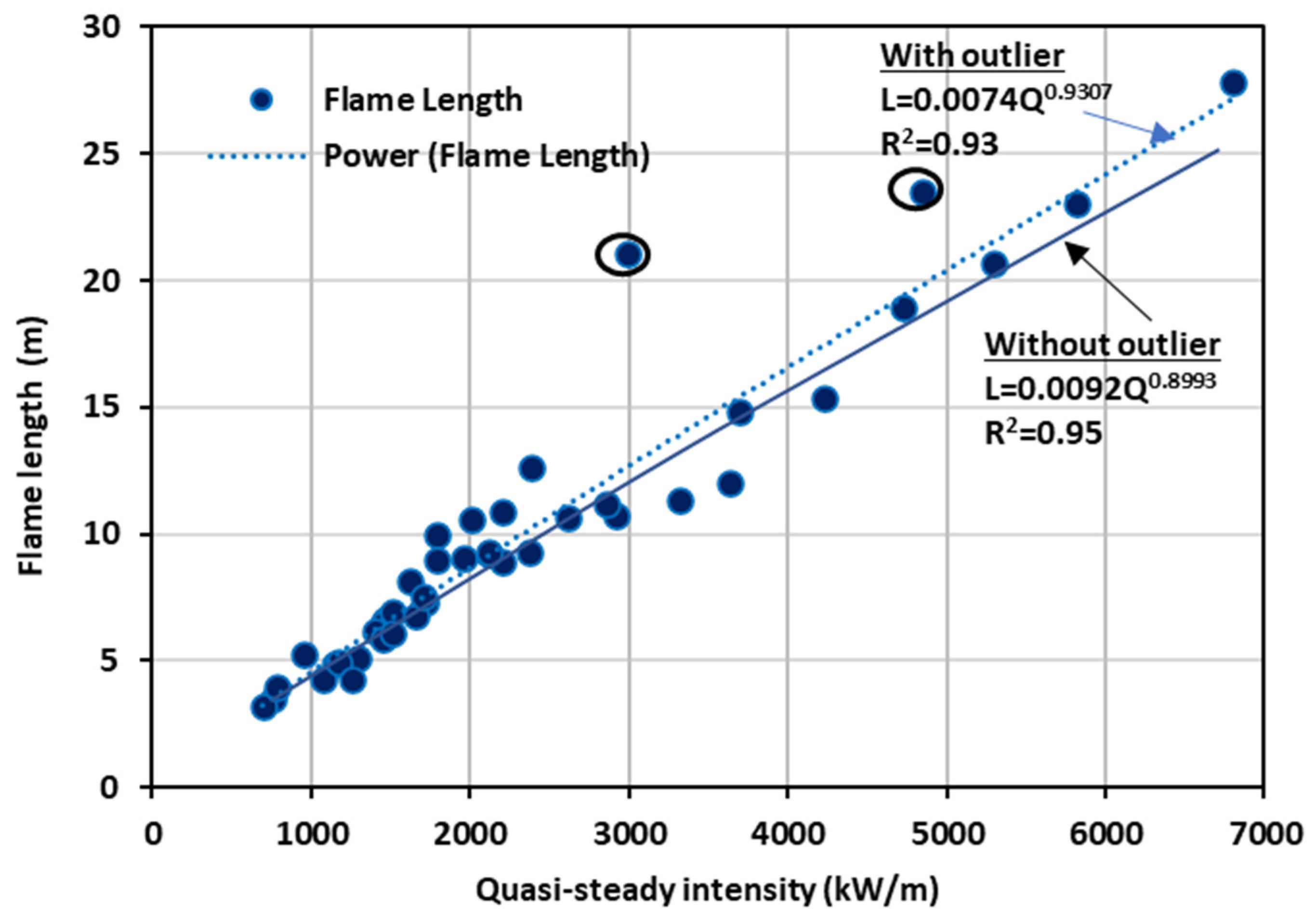
In Figure 13, all simulated L values against Q values for all five velocities, including the values from 12.5, 6, and 3 m/s cases [2], are presented to investigate the correlation for a larger set of wind conditions. A power–law relationship is found to exist when all wind velocities are merged and analysed, in broad agreement with the correlations reported by various experimentalists.

4.7. Heat Fluxes

Following methodology detailed in Section 3, heat flux contour plots, derived from the convective and radiative heat flux boundary data, are presented in Figure 14. Data for scenarios with slope angles of +30°, +20, and +10° at driving wind velocities of 0.1 m/s (Set 1) and 1 m/s (Set 3) are displayed in Figure 14a–c and Figure 14d–f, respectively.
For both lower wind velocities, radiative heat flux contours (red lines) overlap convective heat flux contours (blue lines) for all slope angles. For steeper upslopes, +30° and +20°, radiative heat fluxes are found to lie ahead of convective heat fluxes for both wind velocities where largely buoyancy-driven fire propagation occurs as demonstrated in the Nc analysis in Section 4.5. The same trend is noted for +10° slope as well, though not as predominantly as observed with higher slope angles. The leading or lagging of the fire front by radiative heat flux provides information about where heat transfer occurs as the fire front moves and does not necessarily mean that the total heat flux is dominated by the radiative heat flux.
The total radiative and convective heat fluxes ahead of the fire front are presented in Figure S9 of Annexure A for 0.1 (set 1) and 1 m/s (Set 3) wind velocity. Both the convective and radiative heat fluxes increase with slope angle as well as with the driving wind velocity increases. This is consistent with observations for the higher wind velocities presented in [2]. Evaluating the time series, it is observed that upon establishment of sustained fire fronts, heat fluxes increase as the fire front progresses from the ignition line, then reach a quasi-steady state and finally decrease.
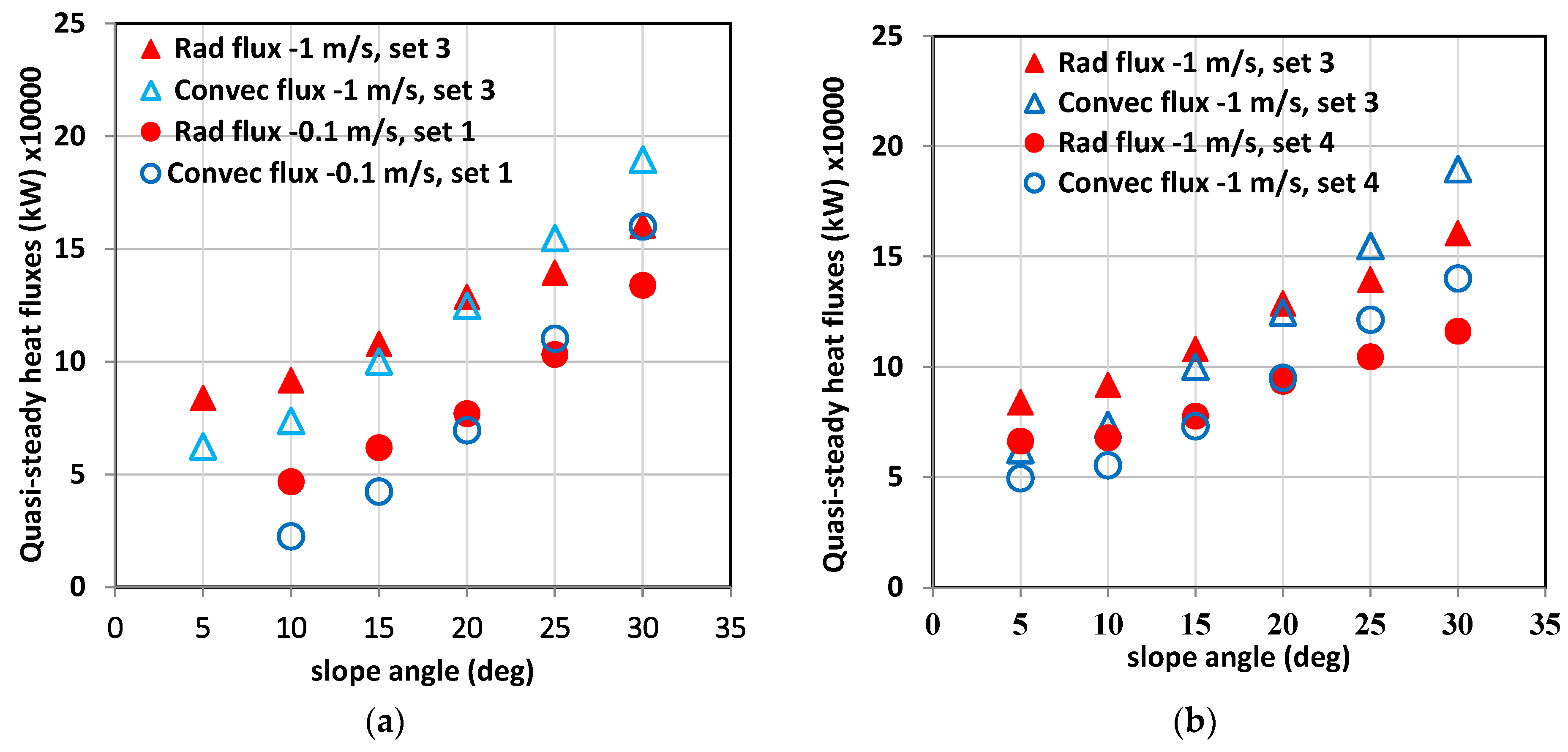
The radiative and convective heat flux values extracted from the quasi-steady region are plotted against slope angles in Figure 15. Heat flux values for wind velocities 0.1 (Set 1) and 1 m/s (Set 3) are presented in Figure 15a, extracted from about 60–300 s for slope angles up to +20° and from about 120–250 s for higher slope angles +25° and +30°. The heat flux values with Set 2 simulations are nearly the same as those with Set 3 (same fuel parameters and wind velocity, different domain size) and therefore Set 2 results are not presented. In Figure 15b, the heat flux values from Set 3 and 4 simulations (original and changed fuel characteristics) are presented. These values are extracted from about 50–200 s for slope angles up to +20° and from about 50–150 s for higher slope angles of +25° and +30°.
From Figure 15, it is evident that for all sets, the total radiative heat flux surpasses the convective heat flux for up to +20° slope. The difference between the fluxes narrows as the slope angle increases, and for higher slopes +25° and +30°, the total convective heat flux overtakes the radiative heat flux. For the +30° slope, the convective heat flux is approximately 20% higher than the radiative heat flux for all sets of simulations. For steeper upslopes, the plume attaches to the ground over a longer distance, resulting in increased convective heat transfer despite the Nc suggesting that all these fires are buoyancy-dominated. Although the boundary conditions, the scale of the fuel bed and fuel type were different, results from this study largely align with the heat flux results observed by Tihay et al. [39] in their experimental investigation (under the no-wind condition). Their heat flux measurements showed that, for a 20° slope, convection represented the major fraction of heat transfer (between 61.1% and 74.9% of the total heat transfer). Similarly, Sánchez-Monroy et al. [30], from their laboratory scale simulation, reported that for no-wind conditions on slopes above +30°, convective heat flux is larger.
For higher wind velocity scenarios [2] the difference between the fluxes decreased as the wind velocity decreased and both fluxes were equally significant at lower driving wind velocity of 3 m/s compared with higher wind velocities. Again, the contour plot of heat fluxes showed that the convective heat fluxes are more relevant at higher upslopes. The results presented in Figure 15 reinforce that at lower wind velocities, the convective heat flux is more relevant at higher slope angles. These results are consistent with the studies of Sánchez-Monroy et al. [30] and Dupuy et al. [38].

5. Summary and Conclusions

In this study, we investigated the intricate dynamics of grassfire propagation, particularly on sloped terrains influenced by low-speed driving winds. Utilizing physical modelling, our exploration highlighted the combined effect of slope and wind on grassfire behaviour at driving wind velocities of 0.1 and 1 m/s. Additionally, we examined variations in domain sizes and fuel characteristics.
Our findings indicate that, generally, the fire isochrones demonstrated similar progression patterns across different velocities, domain size, and fuel characteristics. However, isochrones obtained from “lighter & drier” fuel parameters showed slightly more convex curvatures and thinner pyrolysis widths (or head fire width). Note that simulations with “lighter & drier” were associated with increased ambient temperature and reduced FMC. Similar to our previous studies involving higher wind velocities on sloped terrain [1,2], here also we observe that the fire intensity (Q) rose with the driving wind velocity, given constant fuel characteristics. For a given slope angle, the fire intensity (Q) increased with driving wind velocity, given constant fuel characteristics. However, with the “lighter & drier” fuel, the Q values decreased, similar to the trend noted for pyrolysis width. We noted that fire intensity is directly correlated with pyrolysis width. One of our pivotal observations pertains to the rate of spread (RoS) values, which, when averaged, provided a means to compare with empirical models. A noteworthy finding is the alignment of our quasi-steady and dynamic averaged RoS values with slope-corrected values from renowned empirical models like MK III, CSIRO, and both Rothermel variants. This suggests a promising degree of consistency and reliability in our results compared to established empirical models, especially when considering the error bars and confidence bounds.
Furthermore, our data suggest a transition towards an exponential relationship between RoS and slope angles at lower wind velocities. This resonates with the exponential relationship reported in most of the experimental studies conducted with negligible or very low wind speeds. Similar exponential pyrolysis width–slope and fire intensity–slope relationships were observed.
Our analyses of plume behaviour exhibited a clearly detached or rising plume for upslopes at both these lower wind velocities. Compared with higher wind velocity cases for any given slope angle, the plume was found to rise at a much shorter distance from the ignition line. The Byram number analysis demonstrated that fire propagation was clearly within the buoyancy-dominated regime for these lower wind velocities, whereas near-surface flame dynamics with higher wind velocities were difficult to characterise using the Byram number. With “lighter & drier” fuel characteristics, shorter flame lengths were obtained, as these cases produced lower intensity. For both wind velocities, the flame lengths obtained from this study for <+20° were in reasonably good agreement with the values predicted by the empirical “flame length—intensity” model of Anderson et al. [28].
The contours of the heat fluxes demonstrated that at lower wind velocities, convective heat fluxes are more significant at higher upslope angles. For both wind velocities, the total radiative heat flux surpassed the convective heat flux up to a +20° slope. However, for steeper upslopes, the converse is true.
Overall, this study together with [1,2] provides valuable insights into surface fire behaviour under various combinations of wind, slope, and fuel conditions. Such insights can assist in the improvement of current operational models and thus improve bushfire modelling approaches so that risks and losses associated with bushfires can be reduced. In this series of study, we used WFDS’ boundary fuel model, which may contribute to not spreading fire on downslopes or low upslopes. Future studies might benefit from using the fuel element model, although it may demand significantly more computing power.

Supplementary Materials

The following supporting information can be downloaded at: https://www.mdpi.com/article/10.3390/fire6100406/s1.

Author Contributions

Conceptualization, K.M., D.S. and J.I.; methodology, K.M., D.S. and J.I.; software, D.S. and J.I.; validation, K.M. and D.S.; formal analysis, D.S. and J.I.; investigation, J.I.; resources, K.M.; data curation, K.M., D.S. and J.I.; writing—original draft preparation, J.I.; writing—review and editing, K.M. and D.S.; visualization, D.S. and J.I.; supervision, K.M. and D.S.; project administration, K.M. All authors have read and agreed to the published version of the manuscript.

Funding

This research received no external funding.

Data Availability Statement

Data will be made available when requested.

Conflicts of Interest

The authors declare no conflict of interest.

Abbreviations

AS3959Australian Standard 3959
BFboundary fuel
CFDcomputational fluid dynamics
CSIROCommonwealth Scientific and Industrial Research Organization
FDSFire Dynamic Simulator
FMCfuel moisture content
FEfuel element
GFDIGrassland Fire Danger Index Meter
H R R heat release rate
LESlarge eddy simulation
RoSrate of spread
SEMsynthetic eddy methodology
WFDSWildland–Urban Interface Fire Dynamics Simulator

References

  1. Innocent, J.; Moinuddin, K.; Sutherland, D.; Khan, N. Physics-based simulations of grassfire propagation on sloped terrain at field-scale: Motivations, model reliability, rate of spread and intensity. Int. J. Wildland Fire 2022, 32, 496–512. [Google Scholar] [CrossRef]
  2. Innocent, J.; Sutherland, D.; Khan, N. Moinuddin, Physics-based simulations of grassfire propagation on sloped terrain at field-scale: Flame dynamics, mode of fire propagation and the heat fluxes. Int. J. Wildland Fire 2022, 32, 513–530. [Google Scholar] [CrossRef]
  3. Mell, W.; Jenkins, M.; Gould, J.S.; Cheney, N.P. A physics-based approach to modelling grassland fires. Int. J. Wildland Fire 2007, 16, 1–22. [Google Scholar]
  4. McGrattan, K.B.; Forney, G.P.; Hostikka, S.; McDermott, R.; Weinschenk, C. Fire Dynamics Simulator, User’s Guide, 6th ed.; Original Version 2013, Revised Version 6.3.2 in 2015; NIST Special Publication: Gaithersburg, MD, USA, 2013; p. 1019. [Google Scholar] [CrossRef]
  5. Morvan, D.; Accary, G.; Meradji, S.; Frangieh, N.; Bessonov, O. A 3D physical model to study the behavior of vegetation fires at laboratory scale. Fire Saf. J. 2018, 101, 39–52. [Google Scholar]
  6. Sharples, J.J. Risk Implications of Dynamic Fire Propagation, A Case Study of the Ginninderry Region; Preliminary Report, June 2017; Ginninderra Falls Association: New South Wales, Australia, 2017. [Google Scholar]
  7. Hilton, J.E.; Miller, C.; Sharples, J.J.; Sullivan, A.L. Curvature effects in the dynamic propagation of wildfires. Int. J. Wildland Fire 2016, 25, 1238–1251. [Google Scholar]
  8. Hoffman, C.M.; Canfield, J.; Linn, R.R.; Mell, W.; Sieg, C.H.; Pimont, F.; Ziegler, J. Evaluating Crown Fire Rate of Spread Predictions from Physics-Based Models. Fire Technol. 2015, 52, 221–237. [Google Scholar]
  9. Moinuddin, K.; Khan, N.; Sutherland, D. Numerical study on effect of relative humidity (and fuel moisture) on modes of grassfire propagation. Fire Saf. J. 2021, 125, 103422. [Google Scholar]
  10. Sutherland, D.; Sharples, J.J.; Moinuddin, K.A.M. The effect of ignition protocol on grassfire development. Int. J. Wildland Fire 2020, 29, 70. [Google Scholar] [CrossRef]
  11. McArthur, A.G. Weather and Grassland Fire Behaviour. In Forestry and Timber Bureau; Department of National Development, Commonwealth: Canberra, Australia, 1966. [Google Scholar]
  12. McArthur, A.G. Fire Behaviour in Eucalypt Forests. In Forestry and Timber Bureau; Department of National Development, Commonwealth: Canberra, Australia, 1967. [Google Scholar]
  13. Cheney, N.P.; Gould, J.S.; Catchpole, W.R. Prediction of Fire Spread in Grasslands. Int. J. Wildland Fire 1998, 8, 1–13. [Google Scholar] [CrossRef]
  14. Noble, I.R.; Gill, A.; Barry, G. McArthur’s fire-danger meters expressed as equations. Aust. J. Ecol. 1980, 5, 201–203. [Google Scholar]
  15. Moinuddin, K.; Sutherland, D.; Mell, W. Simulation study of grass fire using a physics-based model: Striving towards numerical rigour and the effect of grass height on the rate-of-spread. Int. J. Wildland Fire 2018, 27, 800–814. [Google Scholar] [CrossRef]
  16. Rothermel, R.C. A Mathematical Model for Predicting Fire Spread in Wildland Fuels; General Technical Report INT-115; Intermountain Forest and Range, USDA Forest Service: Ogden, UT, USA, 1972. [Google Scholar]
  17. Andrews, P.L. The Rothermel Surface Fire Spread Model and Associated Developments: A Comprehensive Explanation; General Techncial Report RMRS-GTR-371; United States Department of Agriculture, Forest Service: Washington, DC, USA, 2018. [Google Scholar]
  18. Wilson, R. Reexamination of Rothermels Fire Spread Equations in No-Wind and No-Slope Conditions; Research Paper INT-434; United States Department of Agriculture, Forest Service: Washington, DC, USA, 1990. [Google Scholar]
  19. Weise, D.; Biging, G. A Qualitative Comparison of Fire spread model incorporating wind and slope effects. For. Sci. 1997, 43, 170–180. [Google Scholar]
  20. Cruz, M.; Alexander, M.E.; Kilinc, M. Wildfire Rates of Spread in Grasslands under Critical Burning Conditions. Fire 2022, 5, 55. [Google Scholar] [CrossRef]
  21. Bishe, E.M.; Afshin, H.; Farhanieh, B. Modified Quasi-Physcial Grassland Fire Spread Model: Sensitivity Analysis. Sustainability 2023, 15, 13639. [Google Scholar] [CrossRef]
  22. Cheney, N.; Gould, J.; Catchpole, W. The Influence of Fuel, Weather and Fire Shape Variables on Fire-Spread in Grasslands. Int. J. Wildland Fire 1993, 3, 31–44. [Google Scholar] [CrossRef]
  23. Byram, G. Combustion of Forest Fuels. In Forest Fire: Control and Use; Davis, K.P., Ed.; McGraw-Hill: New York, NY, USA, 1959; pp. 61–89. [Google Scholar]
  24. Mell, W.; Simeoni, A.; Morvan, D.; Hiers, J.K.; Skowronski, N.; Hadden, R.M. Clarifying the meaning of mantras in wildland fire behaviour modelling: Reply to Cruz et al. (2017). Int. J. Wildland Fire 2018, 27, 770–775. [Google Scholar] [CrossRef]
  25. Morvan, D.; Frangieh, N. Wildland fires behaviour: Wind effect versus Byram’s convective number and consequences upon the regime. Int. J. Wildland Fire 2018, 27, 636. [Google Scholar] [CrossRef]
  26. Dupuy, J.-L.; Maréchal, J. Slope effect on laboratory fire spread: Contribution of radiation and convection to fuel bed preheating. Int. J. Wildland Fire 2011, 20, 289–307. [Google Scholar] [CrossRef]
  27. Alexander, M.E.; Cruz, M.G. Interdependencies between flame length and fireline intensity in predicting crown fire initiation and crown scorch height. Int. J. Wildland Fire 2012, 21, 95–113, Supplementary Erratum in Int. J. Wildland Fire 2021, 30, 70. [Google Scholar] [CrossRef]
  28. Anderson, H.; Brackebusch, A.P.; Mutch, R.W.; Rothermel, R.C. Mechanisms of Fire Spread Research Progress Report No. 2; Research Paper INT-28; US Forest Service: Washington, DC, USA, 1966. [Google Scholar]
  29. Jarrin, N.; Benhamadouche, S.; Laurence, D.; Prosser, R. A synthetic-eddy-method for generating inflow conditions for large-eddy simulations. Int. J. Heat Fluid Flow 2006, 27, 585–593. [Google Scholar] [CrossRef]
  30. Sánchez-Monroy, X.; Mell, W.; Torres-Arenas, J.; Butler, B.W. Fire spread upslope: Numerical simulation of laboratory experiments. Fire Saf. J. 2019, 108, 102844. [Google Scholar] [CrossRef]
  31. AS 3959-2018; Construction of Buildings in Bushfire Prone Area. Australian Standard: Sydney, Australia, 2018.
  32. Overholt, K.J.; Cabrera, J.; Kurzawski, A.; Koopersmith, M.; Ezekoye, O.A. Characterization of Fuel Properties and Fire Spread Rates for Little Bluestem Grass. Fire Technol. 2014, 50, 9–38. [Google Scholar] [CrossRef]
  33. Abu Bakar, A. Characterization of Fire Properties for Coupled Pyrolysis and Combustion Simulation and Their Optimised Use. Ph.D. Thesis, Victoria University, Melbourne, Australia, 2015. [Google Scholar]
  34. Morvan, D.; Dupuy, J.L. Modeling the propagation of a wildfire through a Mediterranean shrub using a multiphase formulation. Combust. Flame 2004, 138, 199–210. [Google Scholar] [CrossRef]
  35. Cheney, N.P.; Gould, J.S. Fire Growth in Grassland Fuels. Int. J. Wildland Fire 1995, 5, 237. [Google Scholar] [CrossRef]
  36. Davis, T.; Sigmon, K. MATLAB Premier, 7th ed.; Chapman & Hall/CRC: Boca Raton, FL, USA, 2005; Available online: www.dbeBooks.com (accessed on 1 June 2017).
  37. Cobian-Iñiguez, J.; Aminfar, A.; Weise, D.R.; Princevac, M. On the Use of Semi-empirical Flame Models for Spreading Chaparral Crown Fire. Front. Mech. Eng. 2019, 5, 50. [Google Scholar] [CrossRef]
  38. Dupuy, J.L.; Mare’chal, J.; Portier, D.; Valette, J.-C. The effects of slope and fuel bed width on laboratory fire behaviour. Int. J. Wildland Fire 2011, 20, 272–288. [Google Scholar] [CrossRef]
  39. Tihay, V.; Morandini, F.; Santoni, P.-A.; Perez-Ramirez, Y.; Barboni, T. Combustion of forest litters under slope conditions: Burning rate, heat release rate, convective and radiant fractions for different loads. Combust. Flame 2014, 161, 3237–3248. [Google Scholar] [CrossRef]
  40. Beck, J.A. Equations For The Forest Fire Behaviour Tables For Western Australia. CALM Sci. 1995, 1, 325–348. [Google Scholar]
  41. Pimont, F.; Dupuy, J.L.; Linn, R.R. Coupled slope and wind effects on fire spread with influences of fire size: A numerical study using FIRETEC. Int. J. Wildland Fire 2012, 21, 828–842. [Google Scholar] [CrossRef]
  42. Sullivan, A.L.; Sharples, J.J.; Matthews, S.; Plucinski, M.P. A downslope fire spread correction factor based on landscape-scale fire behaviour. Environ. Model. Softw. 2014, 62, 153–163. [Google Scholar] [CrossRef]
  43. Mendes-Lopes, J.M.C.; Ventura, J.M.P.; Amaral, J.M.P. Flame characteristics, temperature–time curves, and rate of spread in fires propagating in a bed of Pinus pinaster needles. Int. J. Wildland Fire 2003, 12, 67. [Google Scholar] [CrossRef]
  44. Dold, J.W.; Zinoviev, A. Fire eruption through intensity and spread rate interaction mediated by flow attachment. Combust. Theory Model. 2009, 13, 763–793. [Google Scholar] [CrossRef]
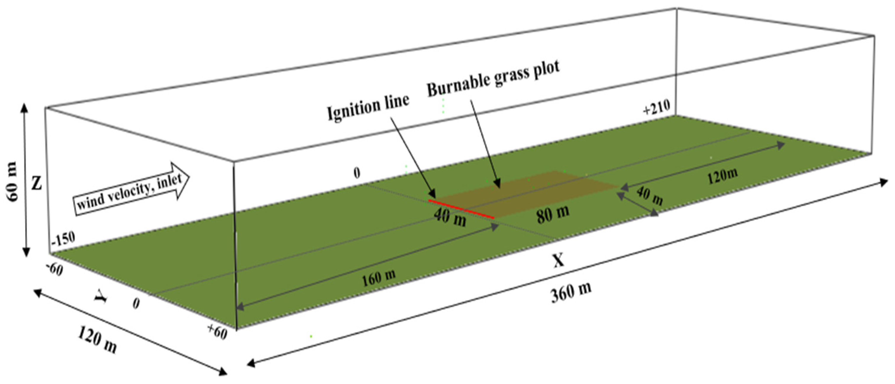
Figure 1. The geometry of the original domain (360 × 120 × 60 m3): The burnable grass plot is 80 × 40 m (olive green region). The same boundary conditions are followed for the larger domain of 480 × 180 × 80 m3.
Fire 06 00406 g001
Figure 2. Progression of isochrones. Frames (ah) original domain at 0.1 m/s (Set 1); Frames (ip) original domain at 1 m/s (Set 2); Frames (qw) large domain, original fuel parameters at 1 m/s (Set 3); and Frames (xad) large domain, changed (“lighter & drier”) fuel at 1 m/s (Set 4).
Fire 06 00406 g002aFire 06 00406 g002bFire 06 00406 g002c
Figure 3. (a) Quasi-steady pyrolysis width vs. slope angle; (b) relative pyrolysis width vs. slope.
Fire 06 00406 g003
Figure 4. Fireline intensity vs. time: (a) quasi-steady intensity vs slope angle; (b) relative intensity vs. slope angle; (c) quasi-steady intensity vs. pyrolysis width.
Fire 06 00406 g004
Figure 5. Fire front location vs. time: (a) Set 1, original domain at 0.1 m/s; (b) Set 2, original domain at 1 m/s; (c) Sets 2 and 3, original and larger domain, at 1 m/s; (d) Sets 3 and 4, original and changed (“lighter & drier”) fuel parameters, at 1 m/s.
Fire 06 00406 g005
Figure 6. RoS—slope angle: WFDS quasi-steady RoS values fitted with a margin of error (95% confidence bounds): (a) at 0.1 m/s (Set 1); (b) at 1 m/s, original fuel parameters (Set 3); (c) at 1 m/s, changed (“lighter & drier”) fuel parameters (Set 4,whiskers look smaller than (a-b) because of the large y-axis range).
Fire 06 00406 g006
Figure 7. Comparison of slope effect: RoS/RoS (+10°) between WFDS results and empirical model values (a) at 0.1 m/s (Set 1); (b) at 1 m/s (Set 3); (c) at 1 m/s (Set 4).
Fire 06 00406 g007
Figure 8. Quasi-steady fire intensity (Q)/fuel load as a function of RoS.
Fire 06 00406 g008
Figure 9. (ac) Plume contour, upslopes at 0.1 m/s (Set 1): +10°, +20°, +30°. (df) Plume contour, upslopes at 1 m/s (Set 3): +10°, +20°, +30°. Plumes emanating from grass plot at +10°, +20°, and +30° upslopes, at wind velocities 0.1 and 1 m/s (Sets 1 and 3).
Fire 06 00406 g009
Figure 10. (ae): +30° at 1 m/s (Set 3). (fj): +10°at 1 m/s (Set 3). (ko): +30°at 0.1 m/s (Set 1). (pt): +10°at 0.1 m/s (Set 1). Flame contour (red) with temperature contour (yellow) in the background along with detachment location (black dot) and wind vector plots (white arrows) at various times.
Fire 06 00406 g010aFire 06 00406 g010bFire 06 00406 g010cFire 06 00406 g010d
Figure 11. Byram convective number (Nc) vs slope angle, derived using quasi-steady RoS, based on U10 at driving wind velocity of 1 m/s; termed as Nc10 in the figure.
Fire 06 00406 g011
Figure 12. (a) Quasi-steady flame length L vs slope with empirically derived values for at 0.1 m/s (Set 1) and at 1 m/s (Set 3); (b) quasi-steady L vs slope with empirical values for Sets 2, 3, and 4 at 1 m/s.
Fire 06 00406 g012
Figure 13. All simulated flame length (L) values against Q values for all five wind velocities: 12.5, 6, 3, 1, and 0.1 m/s.
Fire 06 00406 g013
Figure 14. Instantaneous heat flux contours are taken at different times as the fire front moves through the grass plot: “rad” and “conv” represent radiative and convective heat fluxes, respectively.
Fire 06 00406 g014
Figure 15. Quasi-steady heat fluxes vs slope angles (a) Quasi-steady heat fluxes at 0.1 and 1 m/s—same fuel parameters (Sets 1 and 3); (b) Quasi-steady heat fluxes at 1 m/s—original and “lighter & drier” fuel parameters (Sets 3 and 4).
Fire 06 00406 g015
Table 1. List of simulations.
Slope Angle (Degree) Domain Size:
360 × 120 × 60 M
Domain Size:
480 × 180 × 80 M
Burnable grass plot 80 × 40 m
Wind velocity0.1 m/s, Set 11 m/s, Set 21 m/s, Set 31 m/s, Set 4
Fuel parametersOriginalOriginalOriginalChanged
–10°
+5°
+10°
+15°
+20°
+25°
+30°
Table 2. Thermophysical, pyrolysis, and combustion parameters for grassfire modelling.
Input ParametersValues UsedSource and Reason
Sets 1–3Set 4
Fuel—grass Grass type: kerosene (Eriachne burkittii) [3,15,22]
Heat of combustion16,400 kJ/kg16,400 kJ/kgBluestem grass [32]
Soot yield0.008 g/g0.008 g/gWhite pine (Australian Radiata pine) [33]
Vegetation drag coefficient0.125 assuming vegetation elements are spherical [34]
Vegetation load0.85 kg/m20.31 kg/m2
Vegetation height0.6 m0.6 m
Vegetation moisture content0.0650.024Experimental, Cheney et al. [3,22,35]
Surface area-to-volume ratio of vegetation9770/m 9770/m Experimental, Cheney et al. [3,22,35]
Vegetation char fraction0.170.17Average of Cheney and Gould [22] and Bluestem grass [32]
Vegetation element density440 kg/m3160 kg/m3Australian Radiata pine (Abu Bakar 2015) [33],
hay or straw density
Ambient temperature32 °C50 °CExperimental ([22]), Cheney and Gould [24]
Relative humidity40%10%Experimental [3,22,35]
Emissivity0.990.99Cheney and Gould (1995), [22]
Pyrolysis temperature400–500 K400–500 KMorvan et al. [34]
Degree of curing100%100%Assuming vegetation 100% cured
Heat of pyrolysis200 kJ/kg200 kJ/kgWhite pine (Australian Radiata pine) [33]
Table 3. RoS vs slope angle relationship.
RoSPattern0.1 m/s, Set 11 m/s,
Set 3, Original Fuel
1 m/s (Set 4),
“Lighter & Drier” Fuel
EquationR2Equation R2EquationR2
Dynamic RoS, averageExponential0.0752e0.054x0.9980.1263e0.0411x0.9780.235e0.034x0.984
Quasi-steady RoSExponential0.0711e0.0528x0.9900.1179e0.0405x0.9970.2025e0.0404x0.992
Table 4. RoS percentage changes at every +10° slope.
Slope AngleDriving Wind Velocity
0.1 m/s1 m/s
Set 1Set 3Set 4
+5° to +15°87%60%60%
+10° to +20°87%55%53%
+15° to +25°55%45%50%
+20° to +30°59%45%44%
Table 5. WFDS-relative RoS vs slope angle relationship.
Pattern0.1 m/s, Set 11 m/s, Set 31 m/s, Set 4
Equation R2Equation R2Equation R2
Exponential0.6326e0.0528x0.9900.6675e0.0405x0.9970.6693e0.0404x0.992
Polynomial0.0012x2 + 0.0496x + 0.42240.9950.0007x2 + 0.0309x + 0.62530.9990.0005x2 + 0.0383x + 0.5820.998
Disclaimer/Publisher’s Note: The statements, opinions and data contained in all publications are solely those of the individual author(s) and contributor(s) and not of MDPI and/or the editor(s). MDPI and/or the editor(s) disclaim responsibility for any injury to people or property resulting from any ideas, methods, instructions or products referred to in the content.