Article

Beads and Globules from Fires: Can They Be Differentiated through Metallurgical Analysis Based on Machine Learning Algorithms?

1
Institute of Public Safety Research, Department of Engineering Physics, Tsinghua University, Beijing 100084, China
2
Disaster Accident Investigation Technology Center, Tsinghua University, Beijing 100084, China
3
China Guangdong Nuclear Testing Technology Co., Ltd., Suzhou 215000, China
*
Author to whom correspondence should be addressed.
Fire 2022, 5(4), 123; https://doi.org/10.3390/fire5040123
Submission received: 17 July 2022 / Revised: 16 August 2022 / Accepted: 16 August 2022 / Published: 19 August 2022

Abstract

:
Electrical apparatuses are prone to faults, which generally causes fires. During such fires, the identification of resolidified copper beads on wires has a strong influence on the direction of the fire investigation. There are four kinds of resolidified beads formed on copper conductors that have been through the fire with and without voltage, namely, ‘cause’ beads (CB), ‘victim’ beads (VB), overload globules (OG), and fire melting globules (FG). First, to improve the identification’s objectivity and quantifiability, we used various morphologic parameters of crystals and porosities to express metallurgical microcharacteristics, such as Ar-G, As-G, An-G, Dm-G, R-G, FD-G, Fm-G, Ar-G, As-P, An-P, Dm-P, R-P, FD-P, Fm-P, P3-P, and Cu2O. Then, several machine learning classifiers were developed to predict the melted beads based on metallurgical morphologic parameters by using SVM, BP neutral network (BPNN), AdaBoost, bagging, and random forest (RF), respectively. Models were trained and tested based on the sample set, consisting of 560 samples which were collected from real room fires. ACC/F1 of the RF model were 0.894/0.805, respectively, which are superior to SVM, BPNN, AdaBoost, and bagging. For the RF classifier, the recall rates of CB, VB, OG, and FG were 92.5%, 67.5%, 100%, and 97.5%, respectively, indicating that RF has best potential to predict OG and FG. The variable importance was analyzed to distinguish key features, and the results revealed that Cu2O has highest impact on bead classification. We cannot find much promise with this method that uses multiple metallurgical and morphological parameters for distinguishing between CB and VB. It is confirmed that no machine learning classifiers combined with metallurgical analysis could do this work well in this paper. Thus, we strongly recommend that other evidence for investigation in the room fire should also be considered to cover the shortage of this kind.

1. Introduction

As one of the great disasters of social economy, fire has long been an important problem which requires solving and studying [1,2]. Electrical faults, such as a short circuit or an overload condition, often pose ignition hazards in the easily flammable and environment in daily activities. In order to sum up the lessons learned from fire accidents and to prevent the same accidents from happening again, there is critical need for researchers to investigate the cause of fires accurately and efficiently [3]. In fires, it is known to many investigators that the presence of a rounded mass of resolidified copper means the copper conductor was energized at the time of the fire. However, the tests performed by others demonstrated that beads of resolidified copper may be present on conductors known not to have been energized [4]. In the 2017 edition of NFPA 921, “Guide for Fire and Explosion Investigations”, there are four main resolidified beads formed on copper conductors with and without voltage, namely beads called ‘cause’ beads and ‘victim’ beads, which do or do not start the fires, respectively, and globules that are either caused by overload or by fire melting conditions. Identifying how the resolidified copper beads found in fires were formed plays a crucial role in helping investigators to determine if specific conductors were energized and initiated the fire. An important question for fire investigators is whether these four kinds of beads on copper conductors can be distinguishable from one another.
This question is so critically important to uncovering the truth about fires which has long puzzled investigators and electrical fire researchers. Thus, scholars around the world have begun a difficult quest to find the solution. Henderson et al. [5]. proposed carbon content analysis to identify ‘cause’ beads and ’victim’ beads. The results showed that the carbon content technique is of no value in distinguishing these two kinds of beads. Babrauskas [6] presented some physical and chemical testing methods to distinguish beads that were associated with causing a fire, or were produced as a result of a fire resulting from another cause. He found that relying on the beads’ external shape, surface smoothness, surface roughness, or size was not useful to discriminate ‘cause’ beads and ’victim’ beads. Moreover, unfortunately, energy-dispersive X-ray spectrometry (EDS) was proven insufficient in identifying these two kinds of beads. Wright et al. [4]. had observed both the appearance by stereo microscope and internal microstructures by metallurgical microscopy of beads and globules. It was proposed that beads and globules were similar in appearance, as the surfaces all have fine, rounded, porous structures typical of a solidified solid, but fortunately they could be differentiated by the sharp line of demarcation in their microstructure. NFPA 921 (2017) in Section 9.10.3.2 states that “Beads can be differentiated from globules, which are created by non-localized heating such as overload or fire melting. Beads are characterized by the distinct and identifiable line of demarcation between the melted and the adjacent un-melted portion of the conductor”.
Traditional metallurgical analysis could be used to discriminate beads and globules, but there are still some crucial limitations during its practical use. In the process of investigating electrical fires, resolidified copper beads have most frequently been observed. After metallurgical analysis, it may be concluded that those rounded masses of resolidified copper are beads or globules. However, to determine the cause of fire further, it is difficult to differentiate between ‘cause’ beads and ‘victim’ beads or to identify globules generated by overload or fire attack. This is because the presence of microstructures of beads or globules have close similarity in morphology. Thus, qualitative and semi-quantitative metallurgical analyses, which are mainly relied upon to differentiate the beads or globules at present, have affected the objectivity and accuracy of the prediction results. Therefore, the research in quantitative metallography discrimination of rounded masses of resolidified copper is a pragmatic need for fire investigators.
Methods in computer science offer new methods for microstructure classification. In these approaches, different algorithms and various microstructural parameters are used to build a classification model. DeCost and Holm [7] have applied “the bag of features” to create genetic microstructural signatures that can be used to automatically find relationships in large and diverse microstructural image data sets. Chowdhury et al. [8] have further expanded upon the work presented by DeCost and Holm. Multiple computer vision and machine methods were investigated for microstructure recognition. In addition, they concluded that deep learning algorithms could successfully be applied to micrograph recognition tasks. Bangaru et al. [9] presented a machine learning-based image segmentation method for microstructure analysis. In this work, the results showed that the Random forest (RF) classifier is suitable for microstructure analysis using scanning electron microscopy. Although quantitative microstructural analysis has achieved many advances with the development of computer vision and machine learning, replacing human expertise-based skills by means of computer is still the most challenging part of the process [10]. Hence, a better solution would involve a novel method to meet the fire investigation need. Although there are few researches at present on intelligent quantitative analysis approaches to the determination of metallurgical microstructures, what predecessors in the field have done has laid a solid foundation for exploration of this novel method.
Machine learning has been successfully applied in both fire science [11] and safety areas [12]. For example, ANNs were used to predict forest fires using meteorological data [13], and IV-SVM was used to set up a fire recognition model [14]. Considering our task is to identify the resolidified copper beads in one of four specific categories, some special machine learning methods with advantages of classification were chosen to set up discrimination models. Support vector machine (SVM) is considered in this work because of its simplicity and efficiency. At present, SVM has been a widely used classification and recognition algorithm derived from the statistical learning theory [15,16]. SVM models with different kernel functions can not only solve the classification problems of general data but can also meet the needs of multi-classification problems with small samples and nonlinear characteristics [17]. It is popular in classifying microstructures due to the advantage of its having stronger robustness than other machine learning methods. DeCost and Holm [7] have trained an SVM model in combination with visual features to classify microstructures into one of seven groups with greater than 80% accuracy over five-fold cross-validation. Hence, there is a possibility to use it in discriminating melted beads found in fire scenes. BP (back propagation) neural network is a classic neural network learning algorithm which is also considered in this work. It performed well in stock price pattern classification [18], wear debris classification [19] and identification of bridge grouting compactness [20].
Ensemble methods have been proven to be effective tools for solving multi-label classification tasks [21], and this is why we also considered them as tools to perform beads classification, mainly including boosting, bagging and Random forest. The AdaBoost (the abbreviation of Adaptive Boosting), formulated by Yoav Freund and Robert Schapire [22], is a popular boosting algorithm in ensemble schemes, which perform exceptionally well in classifying soils [23], rock mass [24], and Alcoholic EEG signals [25]. Bagging classifier was used, as it can easily handle higher dimensional data and missing data points and maintains accuracy for missing data. Thus, it is successfully used in the classification of chicken, beef and mutton tissues [26], determinations of COVID-19 CXR images [27], and predictions of credit scoring [28]. Additionally, the Random forest classifier is one of the most successful ensemble learning techniques used for large-sized classification and skewed problems [29]. The Random forest is an ensemble of decision trees, and each tree returns a classification result. Due to its best classification and recognition performance, it has been applied in many different fields, such as heart diseases diagnosis [30], flight departure delay prediction [31], and HCV detections [32].
In our approach, several machine learning algorithms were used to try to meet the challenge of identifying metallurgical images of resolidified copper beads extracted in fires. The task of the discrimination relied on machine learning models previously mentioned. The input and the output were seventeen-dimensional parameter vectors and the bead class labels respectively. The seventeen-dimensional parameters were selected to describe the morphology of the grains and the porosities of the melted beads with the help of Image Pro-Plus 6.0 (IPP 6.0) software. We not only proposed different discrimination models based on different learning algorithms, but also carried out a comparison among them on the accuracy (ACC) and the F1-measure (F1), and then determined a better approach. The rest of this paper is organized as follows: The metallurgical data collection method is introduced in Section 2. In Section 3, several machine learning models are built based on the metallurgical dataset exacted in Section 2, and the prediction results are discussed. In Section 4, the final conclusion is drawn.

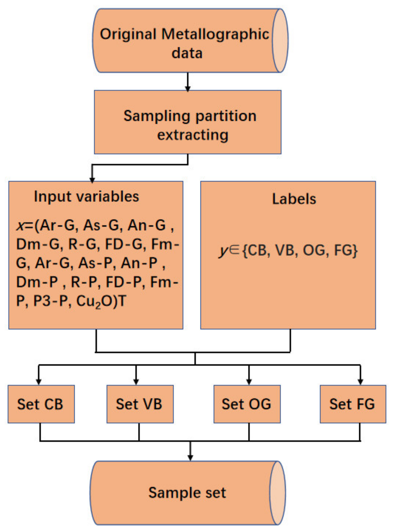
2. The Metallurgical Data Collection

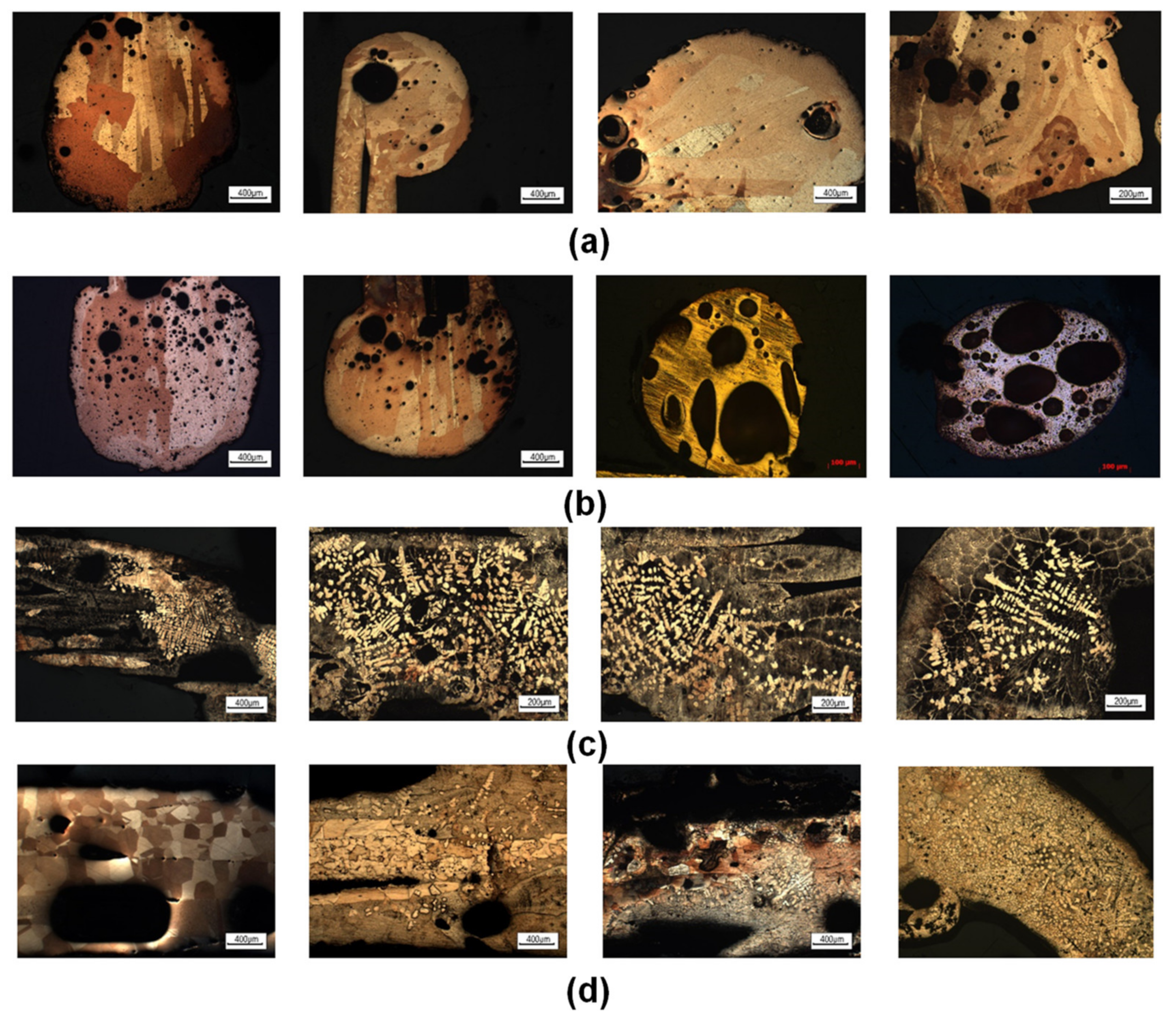
2.1. Experiment Conditions and Metallurgical Image Dataset

In order to establish identification models for analyzing and classifying the metallurgical microstructures of ‘cause’ beads (CB), ‘victim’ beads (VB), overload globules (OG), and fire-melting globules (FG), this process requires a large dataset comprising metallurgical microstructures with different vision angles and at different magnifications. To obtain such a dataset, we collected the resolidified copper beads’ metallurgical images from the Physical Evidence Appraisal Center (PEAC) of China People’s Police University for nearly 10 years, which are used for bead classification as a case study. In such room fires, the copper conductors were exposed to electrical faulting or flames and resolidified as beads or globules. Then we obtained a dataset with 634 images, which was comprised of metallurgical images of CB, VB, OG, and FG. After the filtering process, the dataset containing 560 samples was prepared for analysis. Images were held out into two datasets randomly: a training dataset and a test dataset, corresponding to the models’ training and testing, respectively.
As a result, the training dataset was comprised of micrographs of CB, VB, OG, and FG, which in total included 400 samples, 100 samples for each class. The test dataset was comprised of 160 samples with 40 samples for each class. The examples of metallurgical images of CB, VB, OG, and FG are provided in Figure 1. Columnar crystals and porosities are clearly observed in the metallurgical microstructures of CB and VB. Dendritic morphologies and equiaxed crystals appear in the micrographs of OG and FG. Sometimes, the morphologic characteristics of resolidified copper beads are very similar, which makes it difficult to rely on the quantitative determination of expert prior knowledge traditionally. With the developments of computer vision and machine learning, replacing the experience-based judgment with computer-led processes and realizing the metallurgical microstructures’ automatic discriminations are urgently needed, which will assist investigators to better establish an evidence chain.

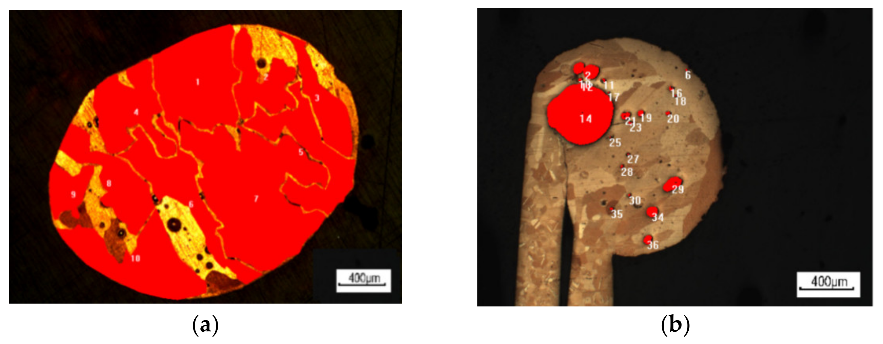
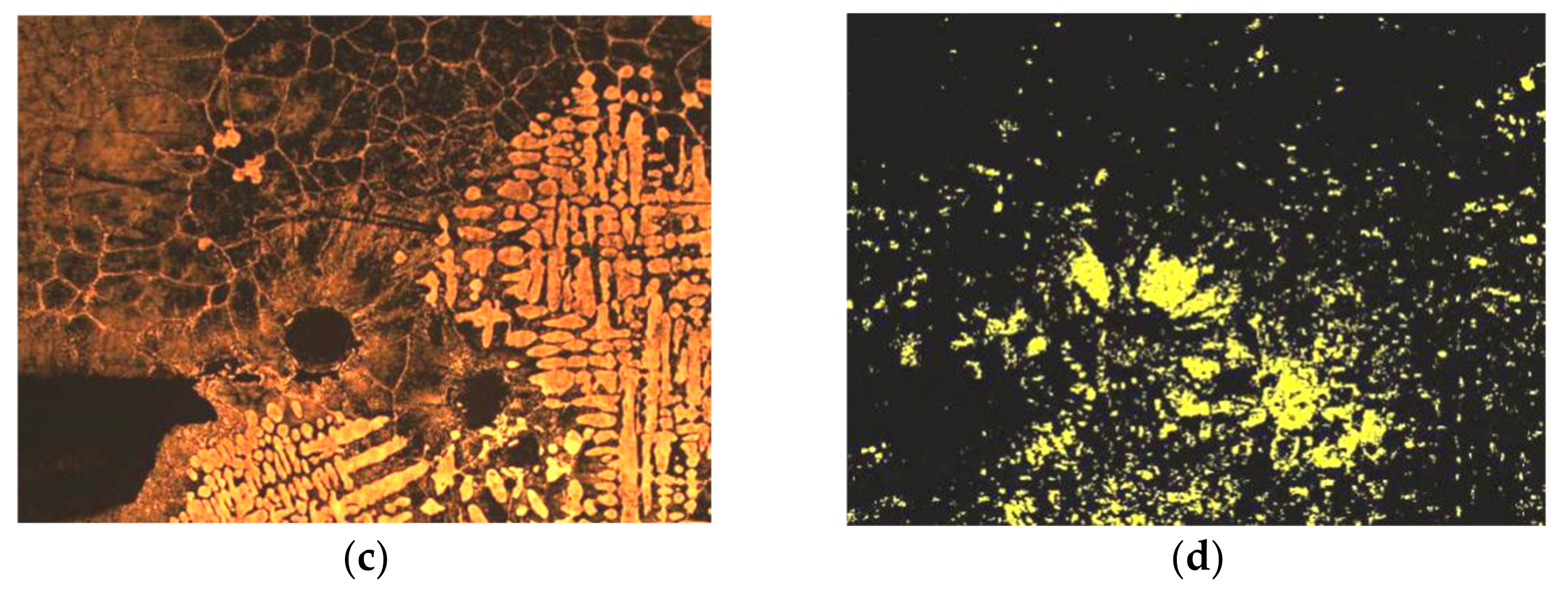
2.2. Selection of Input Variables

The performance of the machine learning model is affected by the number of input variables. Thus, extraction of parameters is the foundation of the determination, and thereby the first step of all procedures. Deng et al. [33] analyzed the metallurgical structures of CB under different short-circuit currents. They found that a strong current was required for Cu2O formation. As the temperature rose, the small grains gradually aggregated and grew, and the dendrites Cu2O and eutectic (Cu + Cu2O) began to form. Hence, Cu2O content was selected as an important dimension of a resolidified copper sample. Based on a real electrical fire, Yu et al. [34] also analyzed the metallographic structure of the arc copper beads, and the average diameter, perimeter, and area of the grains were studied. Li et al. [35] investigated the process and mechanism of breakdown-induced cable insulation exposed to conductor heating caused by overload. Kinds of metallographic microstructure of arc beads were found during a test, such as dendritic segregation structure, equiaxed recrystallized grains and cylindrical crystals. Zhang et al. [36] developed a series of experiments on the glowing contact triggered by poor electrical contacts. They also found that CuO-dominant, Cu2O-dominant, and Cu2O-CuO mixed modes are found in different parts of metallurgical structures. According to NFPA 921, the morphologic structures of grains and porosities are the valid indicators of the resolidification process in fire, thus they may be chosen to describe the characteristics of metallurgical images. The size and shape of grains and porosities vary depending on the solidification behaviors, thus microstructures of melted beads vary widely. Hence, the microstructures of the grains and the porosities are interesting parts of a metallurgical structure. With the help of IPP6.0, we selected seventeen dimensional parameters to represent the morphologic structures of samples mathematically, as shown in Table 1.
The parameters such as area, angle, aspect, diameter (mean), feret (average), fractal dimension, roundness, and perimeter could cover the microstructures of the grains and their porosities comprehensively. The solidification process of beads or globules is a phase-changing process determined by kinetic conditions. When copper solidified, Cu2O formed a grain-like eutectic distribution at the grain boundary, which indicates the heat-treating process of copper conductors in fire. Therefore, we selected the content of Cu2O as one of the important parameters to reflect the recrystallization oxidation degree. The metallurgical microscope was applied to take photographs under the polarized field and IPP6.0 was used for a binary extraction and the measurement of Cu2O content [33]. Each parameter was measured five times in parallel, then averaged. The measurement processes are shown in Figure 2.
The input vectors x derived from metallurgical images had seventeen dimensional parameters. In order to simplify the data processing and to ensure the convergence rate of operation, the input vectors of the training dataset and the test dataset were normalized by the Z-score method into dimensionless variables. Corresponding to this, the output vectors were set which contained the samples’ labels, namely the CB, the VB, the OG, and the FG. Based on these input vectors and output vectors, the models were trained, validated, and tested. Figure 3 shows the data preprocessing procedure. Finally, a dataset with 560 samples was established, in which the number of samples for each class was equal.

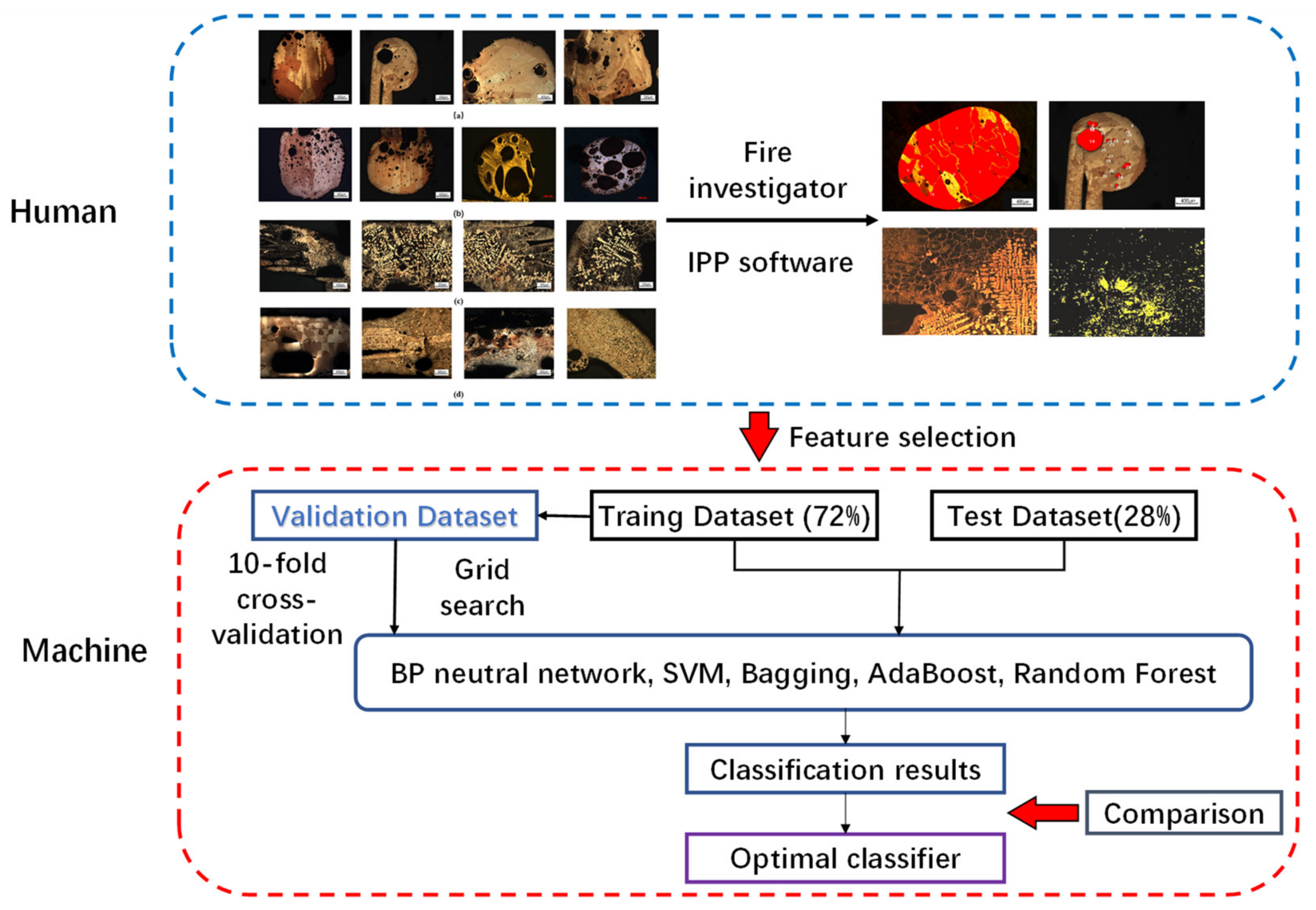
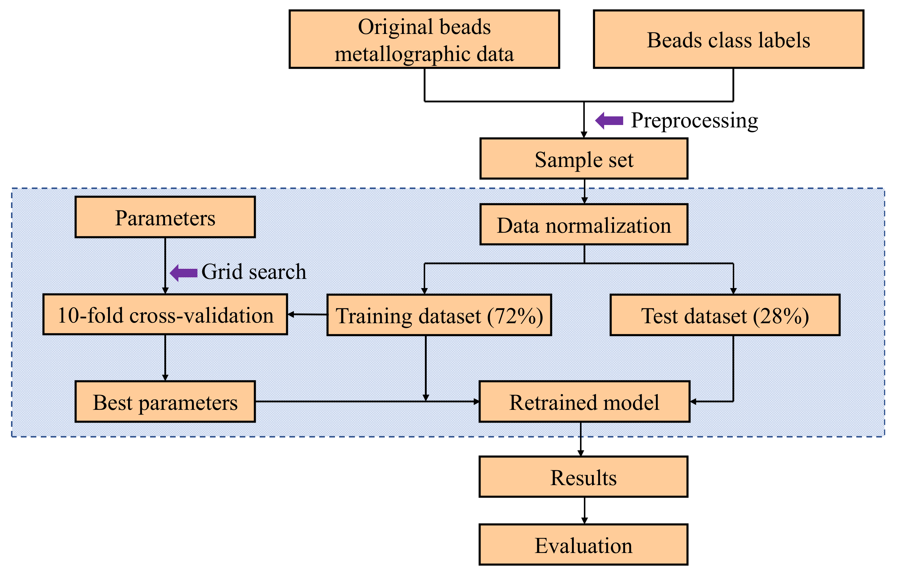
3. Development of Classification Model

Model Training and Evaluation

To obtain a classifier which could perform the bead classification task well, SVM, BP neutral network (BPNN), AdaBoost, bagging, and random forest (RF) were adopted in this research to build such classification models. Then, a comparison was done to choose an optimal one. A flowchart of the bead classification method proposed is shown in Figure 4. In this way, IPP software was used first to select special parameters from each metallurgical image of melted beads which cover the microstructures of grains and porosities comprehensively. Then, the whole dataset was randomly divided into two datasets, namely the training dataset and the test dataset. Then, the five different machine learning algorithms mentioned above were used to set up different bead identification models. Ultimately, the classification results were compared and analyzed, and the model that performed best was identified.
In order to perform this research well, 28% of the whole dataset was used as the test dataset randomly, then the remaining 72% of the metallurgical dataset was kept as the training dataset. The model was trained via 10-fold cross validation, i.e., the training dataset was approximately divided into 10 mutually exclusive subsets, and during each run, the kth subset (10%) was taken as the validation set, while the remaining nine subsets were taken as the training set. Then, the model was evaluated with the average performance of all 10 runs to ensure the stability of the validation results. To obtain the optimal model, the grid search method was utilized during the 10-fold cross-validation process to enumerate the combination of hyperparameters with specified discrete values, as shown in Table 2. After grid-searching, hyperparameters were obtained to make an optimal model which was used to perform the prediction task. A flowchart of model training and testing is shown in Figure 5. Accuracy (ACC) and F1-measure (F1) are adopted as evaluation criteria of the model, and were calculated as follows:
A C C = i = 1 n D i , i / i = 1 n j = 1 n D i , j
F 1 = 1 n F 1 i
F 1 i = 2 P i R i P i + R i
P i = D i , i k = 1 n k , i
R i = D i , i k = 1 n i , k
where D represents the confusion matrix, D i , j represents the number of samples with real class i and predicted class j, F 1 i , P i , and R i represent the F1-measure, accuracy, and recall (R) of class i, respectively, and n represents the number of classes. The values of ACC and F1 ranged from 0 to 1, with 1 representing the best model performance and 0 the poorest.

4. Results and Discussion

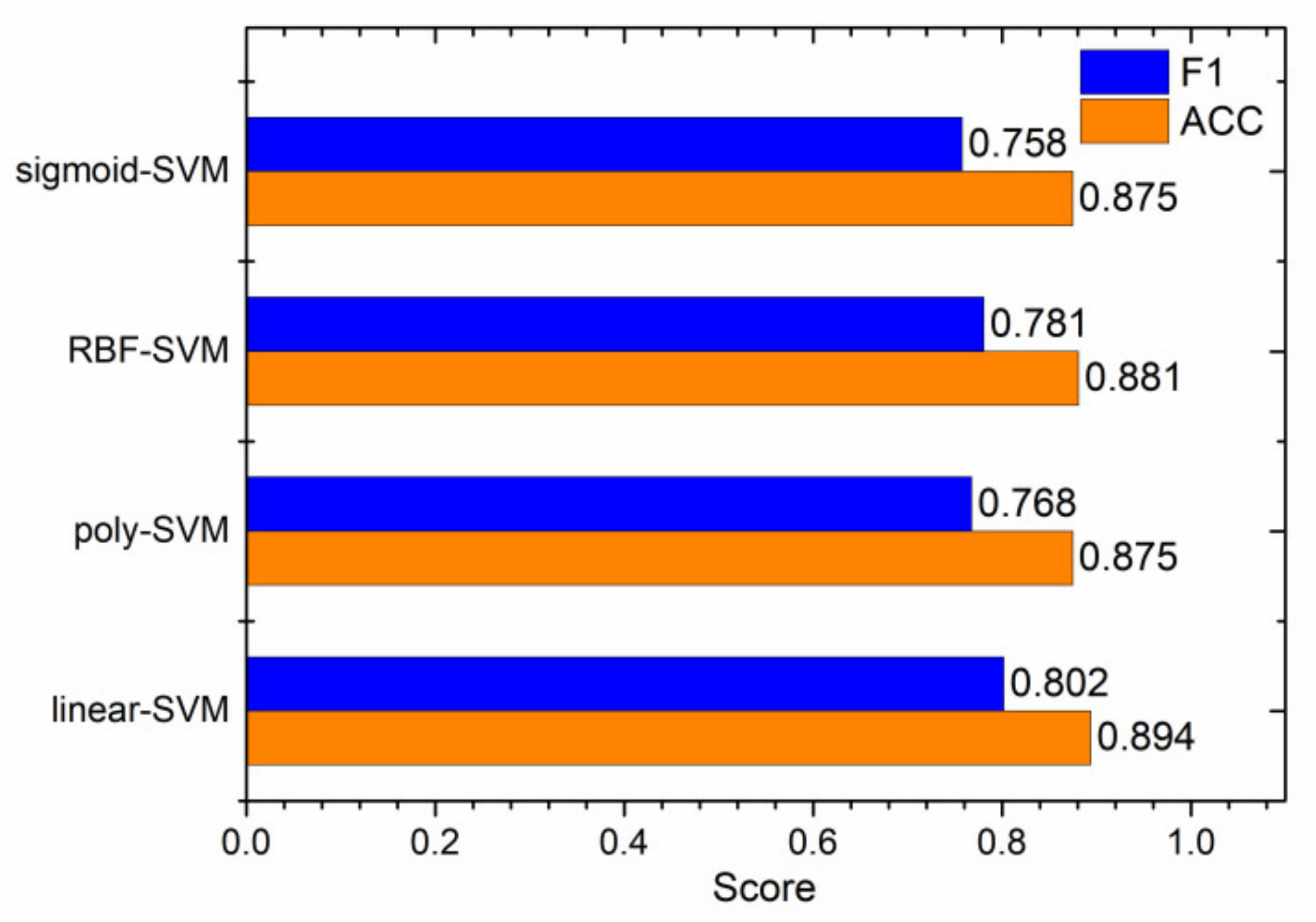
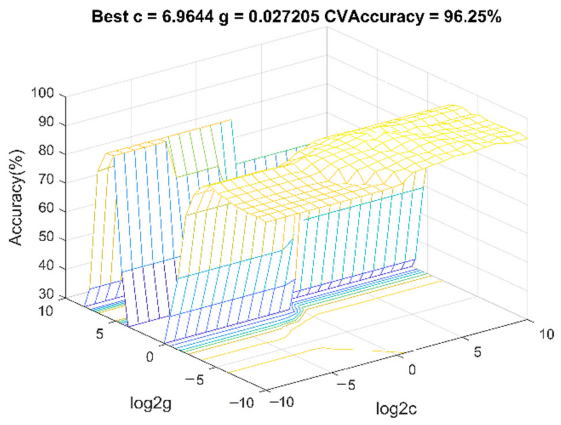
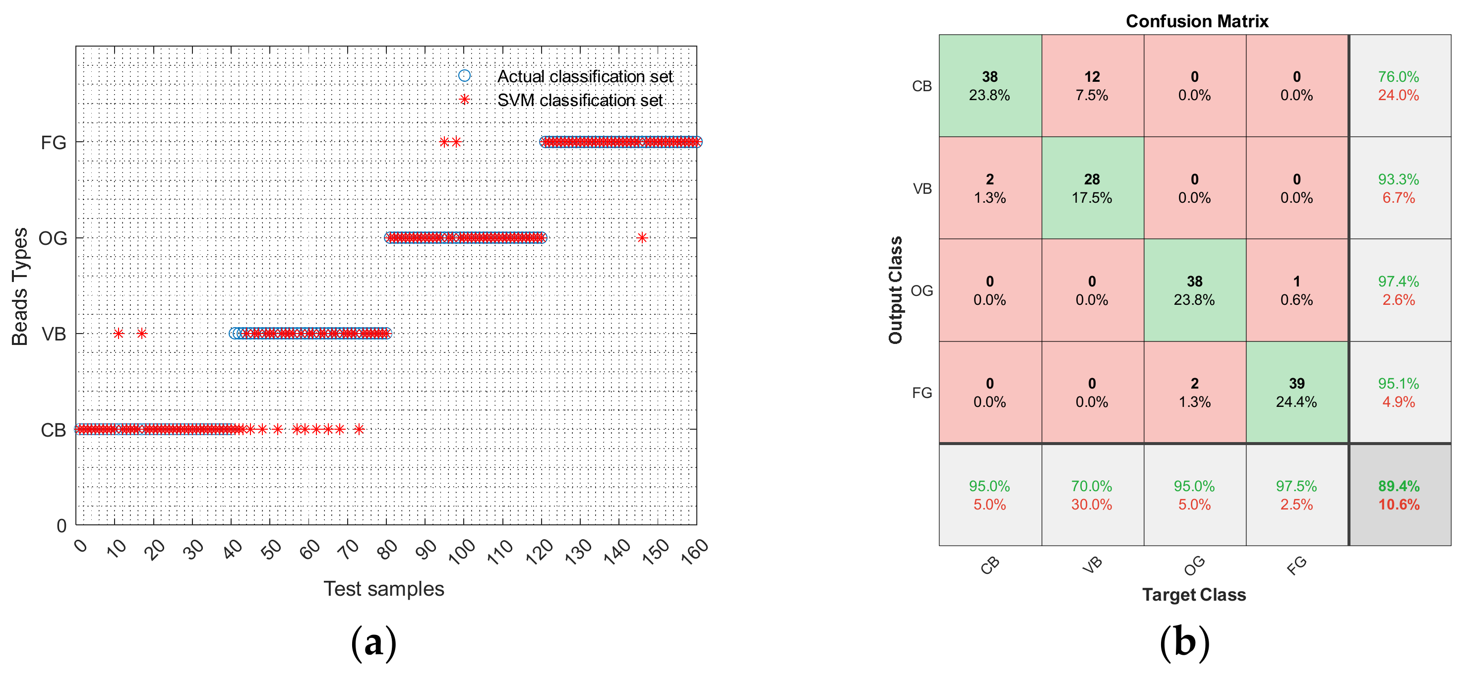
4.1. Prediction Results of SVMs

The primary target of SVM models is to maximize the margin among all these classes. SVM is a supervised classifier with a special kernel function to find the best hyperplane that separates the training samples of targeted classes. In this work, linear kernel function, polynomial kernel function, RBF kernel function, and sigmoid kernel function were carried out to find the best hyperplane. Firstly, the input vectors of the training dataset were found to determine the optimal penalty parameter c and kernel function width g by using the grid search method. At the same time, the 10-fold cross-validation method was performed to validate the model’s performance. The ACC/F1 of linear-SVM, poly-SVM, RBF-SVM, and sigmoid-SVM were 0.894/0.802, 0.875/0.768, 0.881/0.781, and 0.875/0.758, respectively, as shown in Figure 6. The performance of linear-SVM exceeded that of other SVM models.
Figure 7 shows the results of linear-SVM hyper-parameters selection by using the grid search method. It was determined that c was 6.96 and g was 0.03, with the 10-fold cross-validation accuracy of 96.25%.
Figure 8a represents the classification results of the linear-SVM model. Evidently, none of the beads were classified into globules. However, seventeen prediction errors occurred. Namely, there were three CB samples misclassified into VB, while thirteen VB samples were misclassified in CB. Additionally, one FG sample was classified into OG. The confusion matrix in Figure 8b graphically shows the linear-SVM classification performance with respect to each individual class. The vertical axis corresponds to the class predicted by the SVM classifiers, and the horizontal axis corresponds to the actual class of each test sample. The recall rates of CB, VB, OG, and FG are 0.975, 0.625, 1, and 0.975, respectively. This is principally because columnar crystal structures and porosities appear in both VB and CB, which leads to difficulty in differentiating them due to their similar morphological characteristics. In addition, the recrystallization processes of VB and CB are similar because they are both arc beads, which determines that these two groups of copper beads have similar levels of Cu2O. The misclassification between OG and FG is because dendritic morphologies occasionally appear in FG microstructures. In contrast, no beads were classified as globules, and no globules were differentiated as beads.

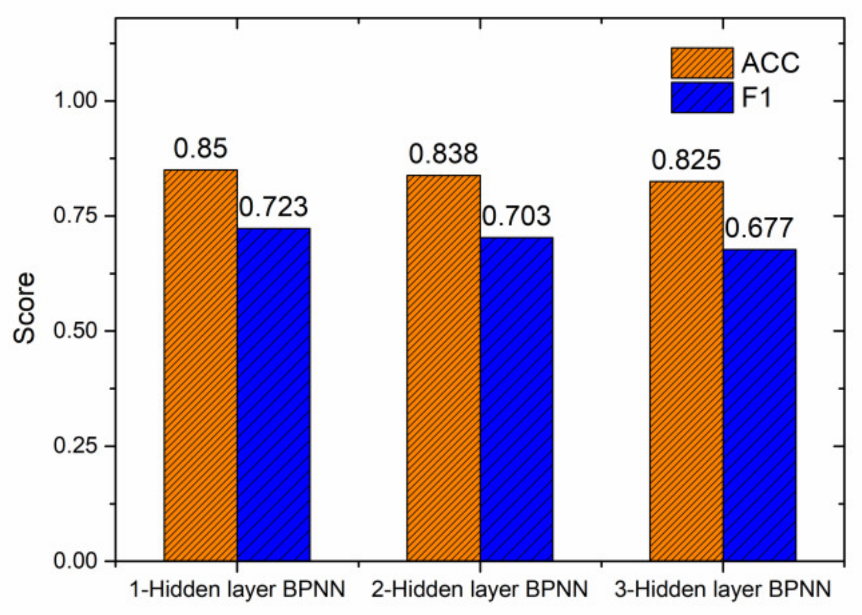
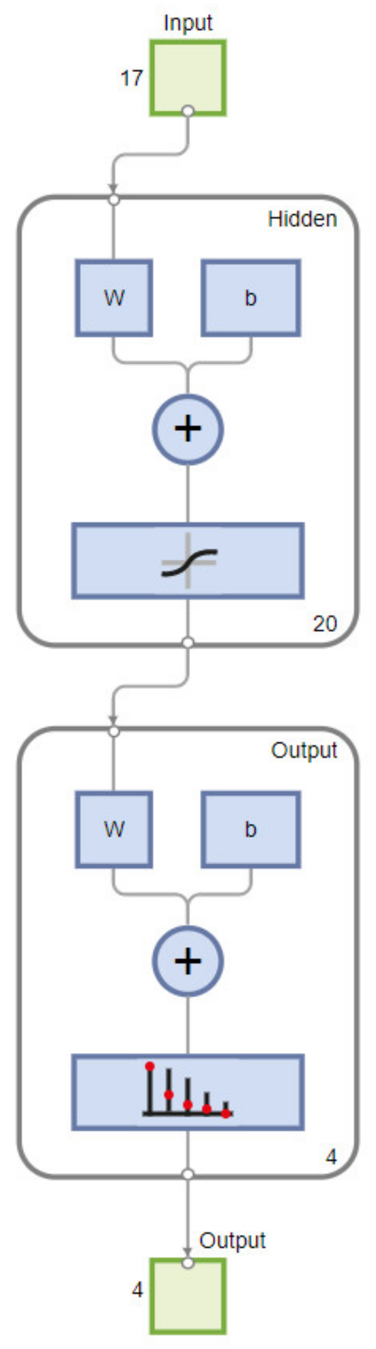
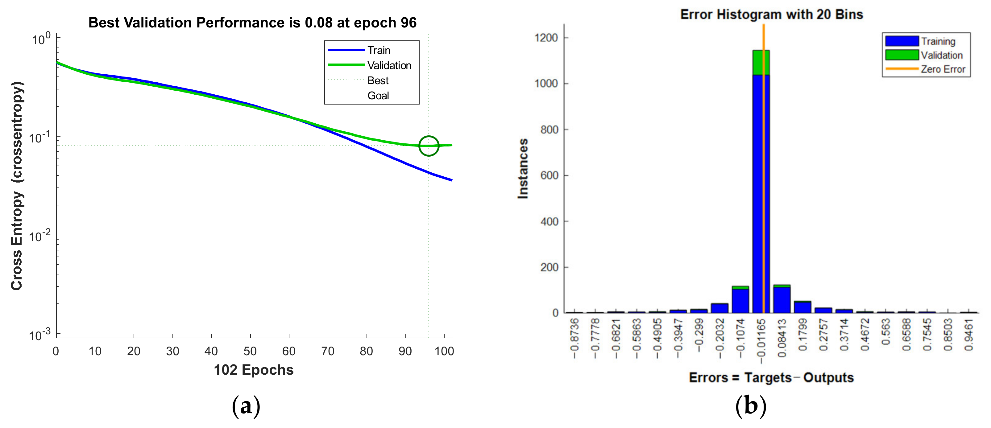
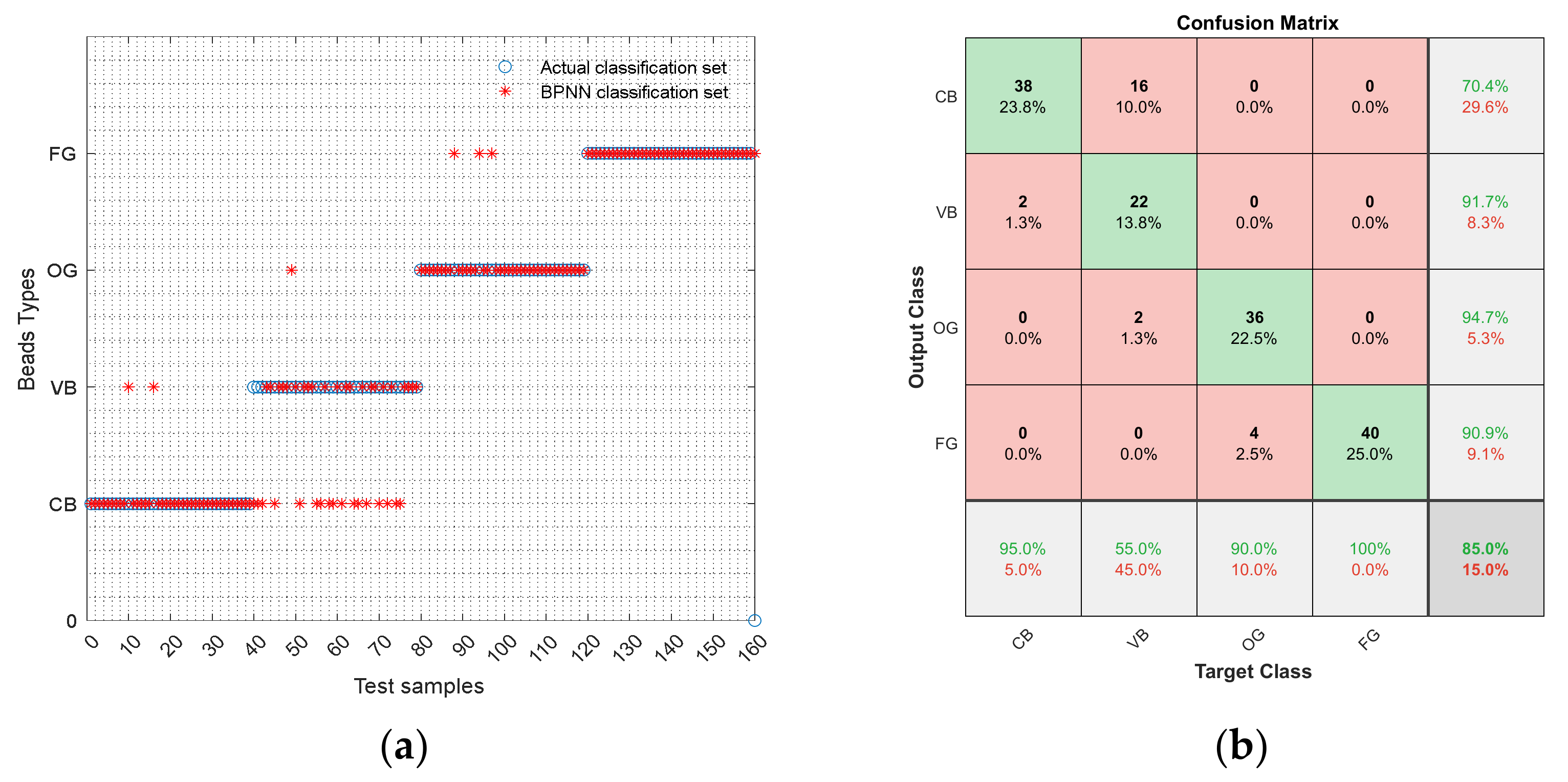
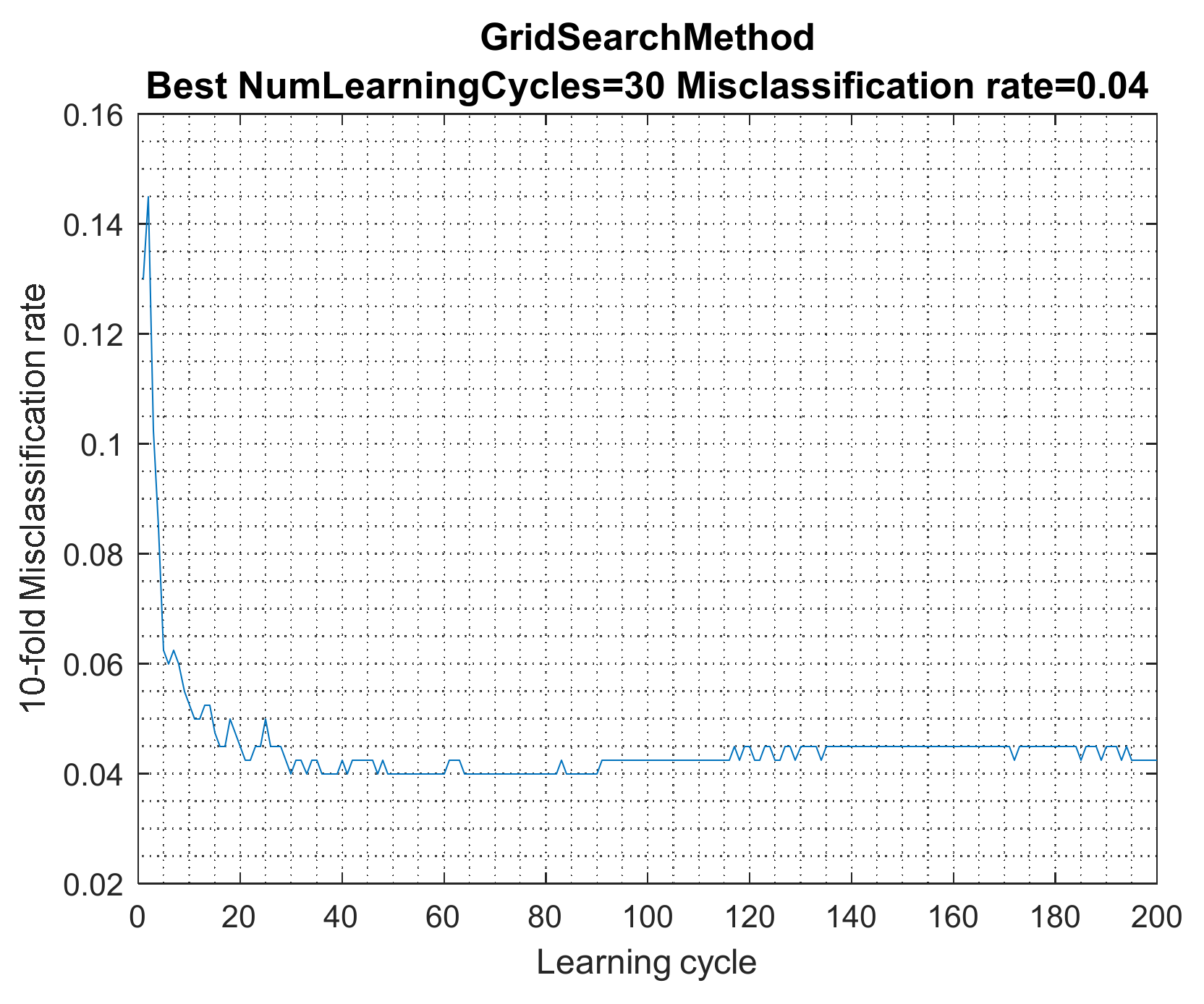
4.2. Prediction Results of BPNN

BPNN has been widely used in prediction works such as ash melting characteristic temperature [37], landslide [38], and PM 2.5 mass concentration [39]. Hence, it was also considered in this paper for the task of performing bead predication. The training function of the BPNN is a gradient-descending function based on a momentum and an adaptive learning rate. The learning algorithm of the connection weights and the threshold values is a momentum-learning algorithm based on gradient descending. The performance of the BPNN is affected by the number of hidden layers, hidden layer size, train function, and transfer function. To obtain the optimal model, the grid search method was utilized to evaluate the combination of parameters with special discrete values, as shown in Table 2. The process of parameters selection and model validation is shown in Figure 5. 10-fold cross-validation was also performed on the training dataset, combined with the grid search method, to select proper parameters of the model. Early stopping was used as the stop criteria in the BPNN model. It means that in the process of network training, if cross-entropy validation curve does not decrease for 6 consecutive iterations, training process is stopped.
After grid search and model validation, we found that when the values of the number of hidden layers, the nodes of hidden layer, the train function, and the transfer function were 1, 20, traingdx, and logsig, respectively, a BPNN model could perform this work well. It is worth mentioning that, in terms of this fire investigation issue, the validation accuracy could not increase by adding hidden layers. More hidden layers may even lead to an over-fitting issue. The ACC/F1 of 1-Hidden layer BPNN, 2-Hidden layer BPNN, and 3-Hidden layer BPNN were 0.850/0.723, 0.838/0.703, and 0.825/0.677, respectively, as shown in Figure 9. Evidently, the performance of 1-Hidden layer BPNN exceeded those of other multi-Hidden layer BPNN models.
Hence, the 3-layer BPNN was ultimately adopted in this paper, whose diagram is shown in Figure 10. Figure 11a shows the process of the grid search and validation. The model’s 10-fold validation misclassification rate was 0.08. Figure 11b clearly demonstrates the error histogram during the cross-validation. Evidently, all of the errors were quite low and fell between the range of −0.8736 to 0.9401, but most of the errors fell between the range of −0.299 to 0.2757 where high bars could be clearly seen.
Figure 12a demonstrates the classification results of the BPNN algorithm. Distinctly, it is found that there were twenty-four prediction errors of BPNN model. Namely, there are two CB samples misclassified in VB, while sixteen VB samples were misclassified in CB. Additionally, there were two VB samples misclassified in OG. Moreover, four OG samples were misclassified in FG. Figure 12b shows the BPNN’s classification performance. The recall rates of CB, VB, OG, and FG are 0.95, 0.55, 0.90, and 1, respectively. Unfortunately, BPNN does not distinguish VB from VB well.

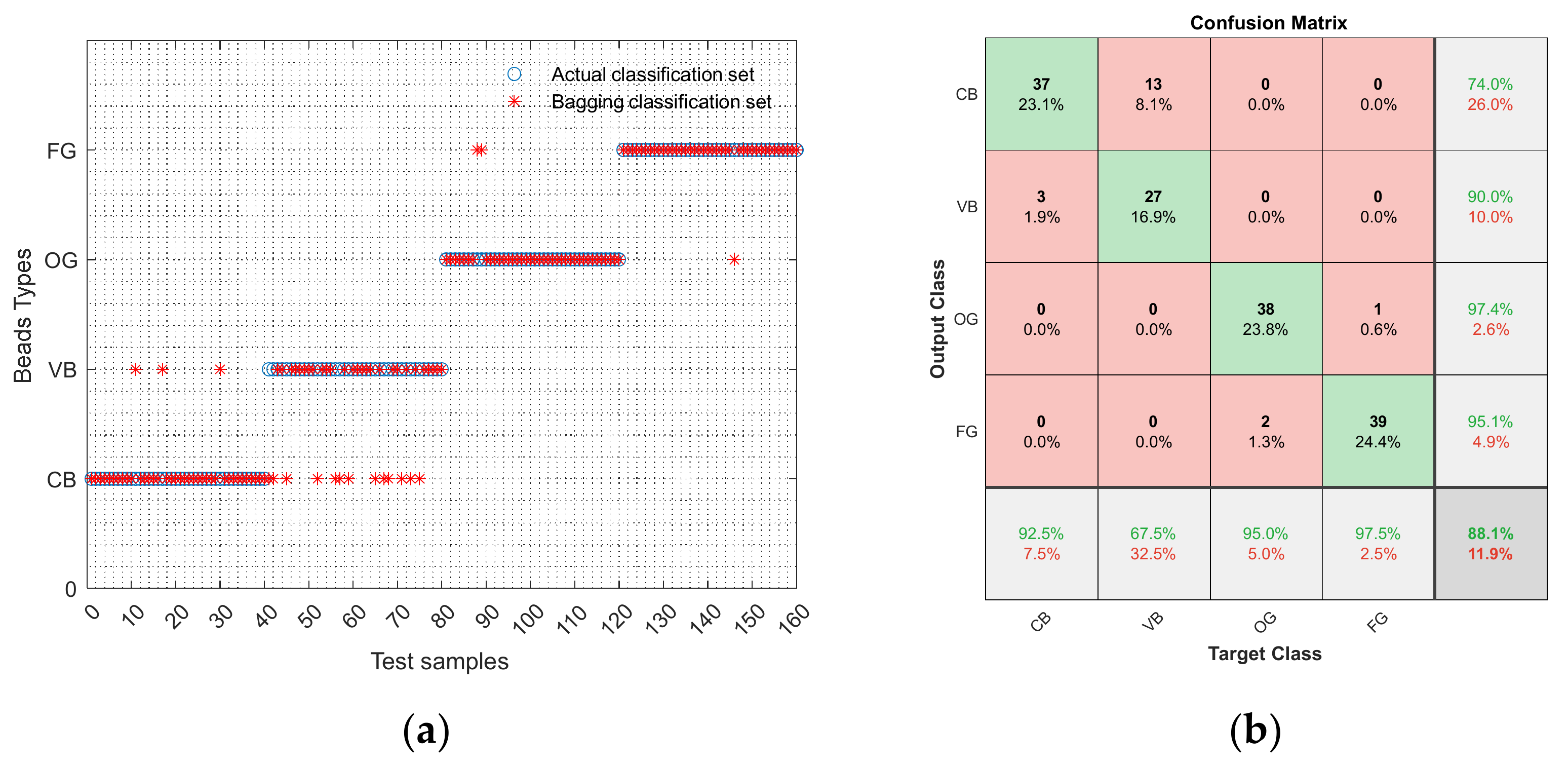
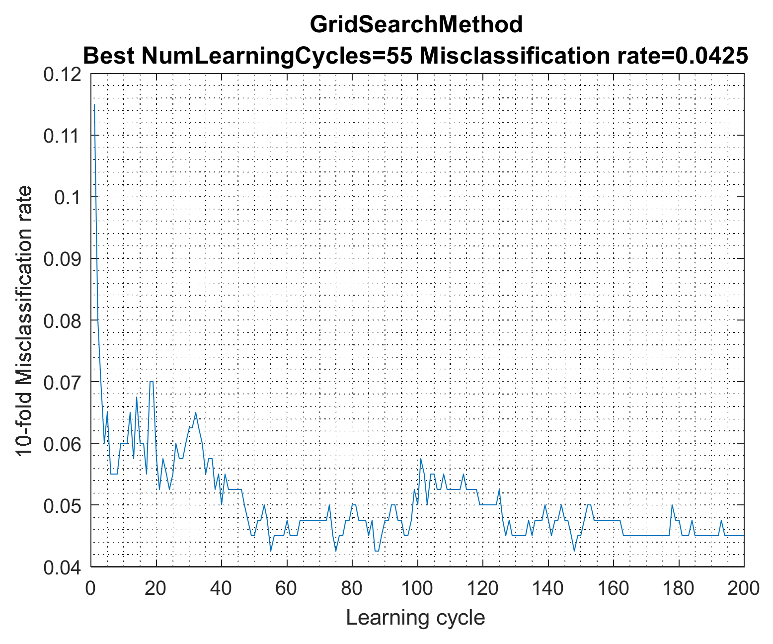
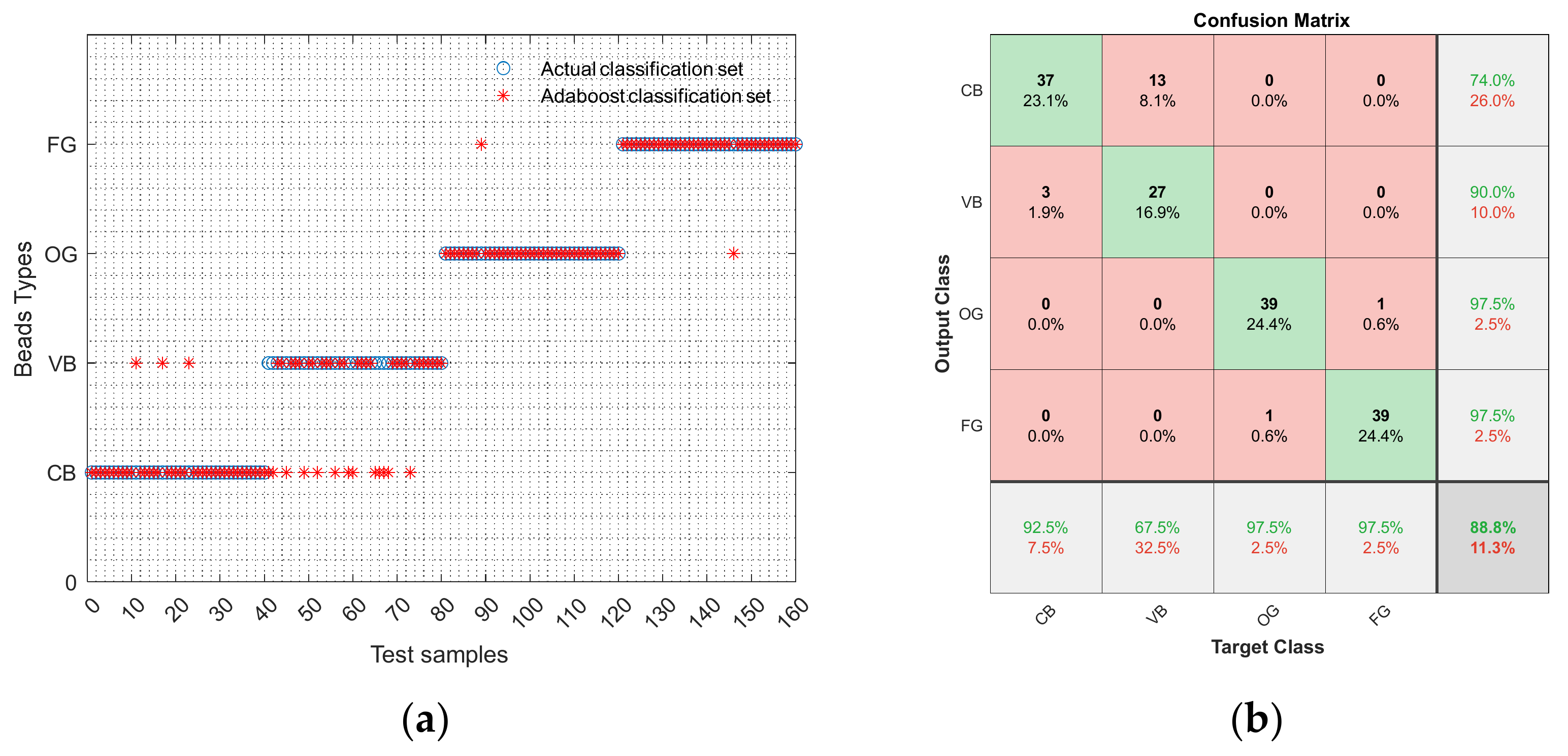
4.3. Prediction Results of Bagging and AdaBoost

This study also adopted AdaBoost and bagging as the classifiers to perform this prediction task. Bagging and boosting yield N learners by generating additional data in the training stage. N new training data sets are produced by random sampling with replacement from the original set. In the case of bagging, any element has the same probability of appearing in a new data set. However, for boosting the observations are weighted, AdaBoost is a genetic iterative supervised learning algorithm that combines weak hypotheses in a much more accurate master hypothesis. AdaBoost M2 algorithm [22] was used in this work.
The decision tree algorithm was used as the base classifier for these two kinds of classifiers, and the models were trained and validated via 10-fold cross-validation by using the same process as shown in Figure 5. The performances of both AdaBoost and bagging are affected by the number of base classifiers, namely the NumLearningCycles in these two algorithms. In this work, due to a relatively small training dataset, we used some default values of parameters of the decision tree. For the bagging algorithm, the maximal number of decision splits (MaxNumSplits) was 399, while for AdaBoost, MaxNumSpilts was 10. For bagging and AdaBoost, minimum observations per leaf (MinLeafSize) was set as 1. In order to find a proper value of NumLearningCycles of bagging and AdaBoost, the grid search method was used. Figure 13 shows the grid search results of bagging; it was found that when NumLearningCycles was 30, bagging had the lower 10-fold misclassification rate of 0.04.
Figure 14a shows the prediction performance of bagging. There were nineteen prediction errors. Moreover, there were three VB samples misclassified as CB samples, while thirteen VB samples were wrongly divided into CB. In addition, two OG samples were falsely classified as FG, and one FG sample was misclassified in OG. Figure 14b shows the classification performance of the bagging. The recall rates of CB, VB, OG, and FG are 92.5%, 67.5%, 95%, and 97.5%, respectively.
Figure 15 demonstrates the grid search results of AdaBoost, showing that when NumLearningCycles was 55, the 10-fold misclassification rate was 0.0425.
As shown in Figure 16a, it is clear that there were eighteen prediction errors. Namely, there were three CB samples misclassified as VB samples. At the same time, thirteen VB samples were misclassified as CB samples. It is worth noting that only one OG sample was determined in FG class and one FG sample was misclassified as an OG sample. AdaBoost’s classification performance is shown in Figure 16b. The recall rates of CB, VB, OG, and FG are 92.5%, 67.5%, 97.5%, and 97.5%, respectively. In conclusion, the AdaBoost algorithm has a good performance in predicting OG and FG.
The ACC/F1 of bagging and AdaBoost were 0.881/0.781 and 0.888/0.793, respectively. Clearly, AdaBoost achieved a better performance than bagging in predicting OG with the recall rate of 0.975. For CB, VB, and FG, these two classifiers have the same prediction ability with the recall rates of 0.925, 0.675 and 0.975, respectively. Besides, AdaBoost and bagging both have poor performance in predicting VB. Principally, it is because the metallurgical microstructures of CB and VB are similar. Through metallurgical analysis, it can be observed that the morphological characteristics of copper grain crystals and pores in CB and VB are difficult to distinguish. If there is no definite boundary between different classes, the model cannot accurately identify the samples. Hence, differentiating between CB and VB is still a challenge in the fire investigation field.

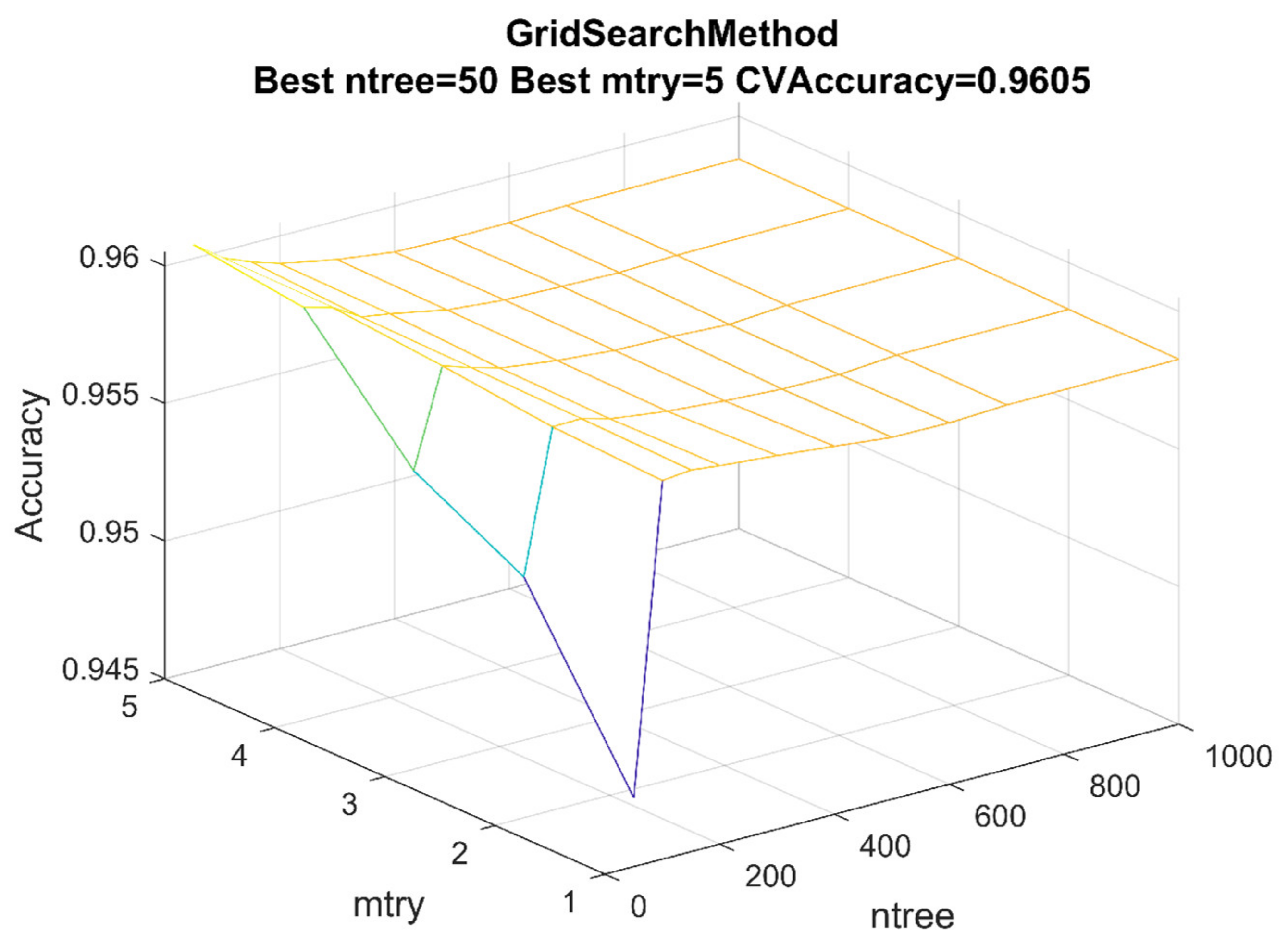
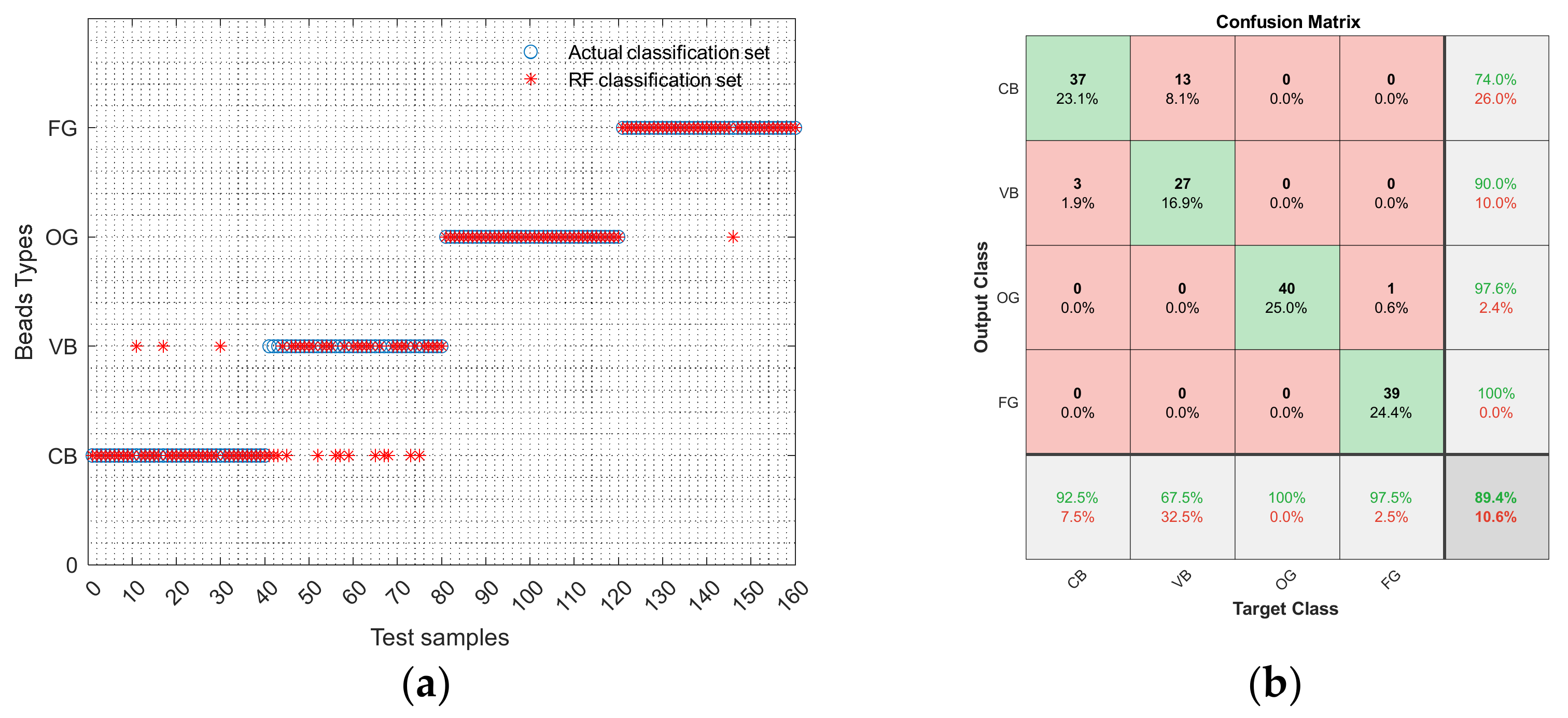
4.4. Prediction Results of RF

RF is an ensemble learning algorithm that performs by constructing a multitude of decision trees at training time and outputting the class. Moreover, it is an extension of bagging that also randomly selects subsets of features used in each data sample.
Here, we employed the RF as the classifier to differentiate the melted copper beads. Each CART-decision tree in the RF was built using a bootstrap sample with replacement from the original data, which helped to reduce the variance of the algorithm and avoided over-fitting. In this RF algorithm, 10-fold cross-validation was performed using the training dataset, and the test dataset was used to test. The model’s training, validation, and test process are shown in Figure 5. According to the statistical mechanism of RF, the most important parameters include mtry and ntree, which have a significant impact on the prediction performance. These two parameters, mtry (i.e., the number of input variables randomly chosen at each spilt) and ntree (i.e., the number of trees to grow for each forest) were determined by the grid search method, shown in Figure 17. When ntree and mtry were 50 and 5, respectively, the model’s validation performance was best.
As shown in Figure 18a, there are three CBs misclassified as VBs, while thirteen CBs were divided into VB class wrongly. One FG sample was classified as OG class. Notably, all OG samples were predicted appropriately. The confusion matrix of RF was as shown in Figure 18b. In general, RF had the better predication performance, with a high accuracy rate at 89.4%. For CB, VB, OG, and FG, the recall rates were 92.5%, 67.5%, 100%, and 97.5%, respectively. The above evidence shows that RF has great potential to differentiate the resolidified copper beads found in fire. Through the ACC/F1 comparison between bagging (0.881/0.781) and RF (0.894/0.805), it was revealed that the performance of RF exceeded that of bagging.
However, it can be observed that RF also has a poor ability to distinguish VBs from CBs. In summary, the main reason for this is that the morphological difference between CB and VB is nonapparent. Unfortunately, relying on metallurgical data alone will not assist fire investigators in determining resolidified copper beads that do or do not start a fire. Other evidence of investigation in an electrical fire is strongly recommended, such as video surveillance information, trace of the fire, and a witness statement.

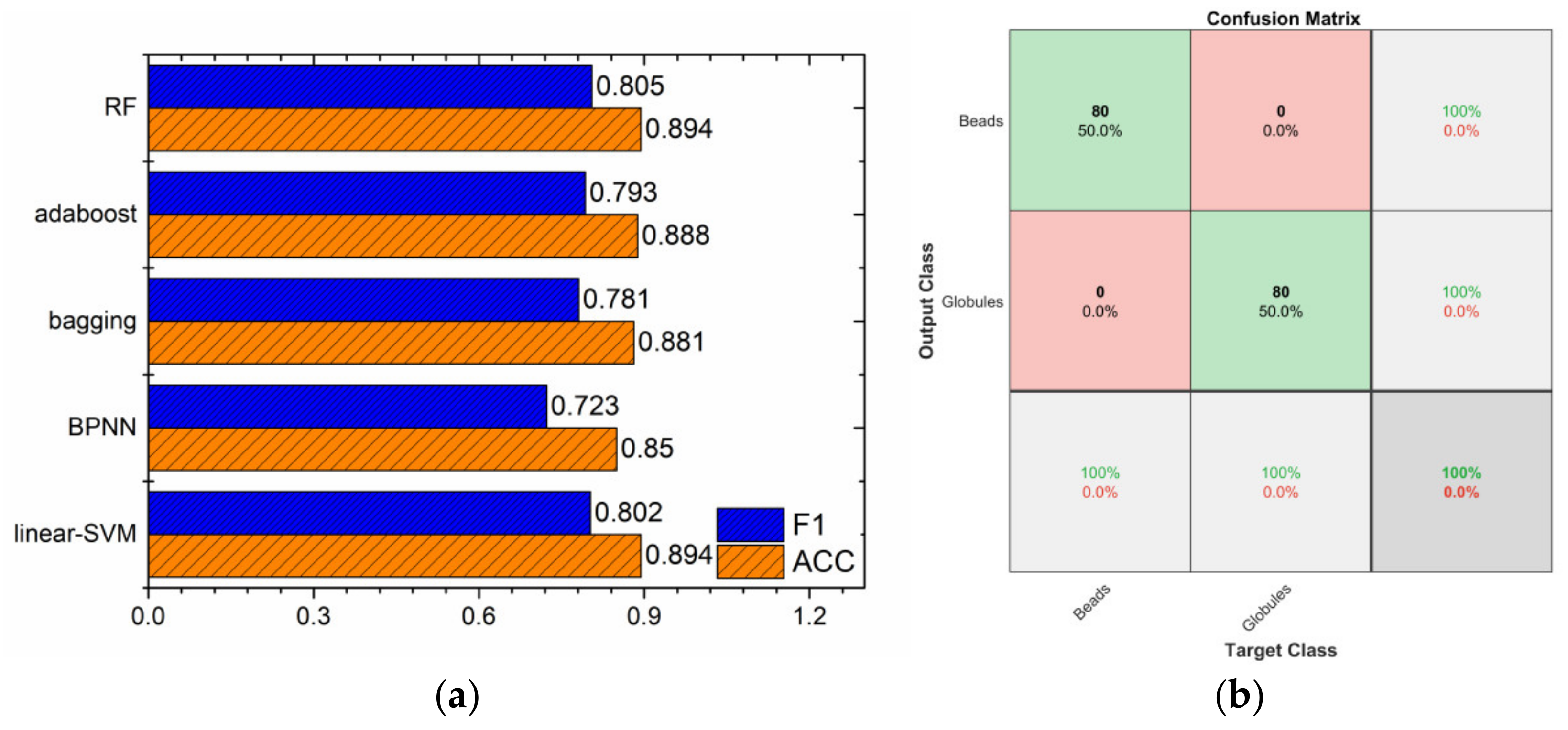
4.5. Performance Comparison among Classifiers

In this work, several excellent machine learning classifiers have been adopted to carry out the resolidified copper beads classification missions using the same dataset. All models were developed using the same process in Figure 5. Figure 19a represents the comparison results of model performance. Distinctly, the ACC/F1 of linear-SVM, BPNN, bagging, AdaBoost, and RF were 0.894/0.802, 0.850/0.723, 0.881/0.781, 0.888/0.793, and 0.894/0.805, respectively. The performance of RF exceeded that of other models. It is worth mentioning that the misclassification between CB and VB is because columnar crystal structures and porosities appear in both of them. In addition, the recrystallization processes of VB and CB are similar, which determines that these two groups of copper beads have similar levels of Cu2O. Furthermore, the misclassification between OG and FG is because dendritic morphology occasionally appears in FG microstructures. Fortunately, linear-SVM, bagging, AdaBoost, and RF used in this work could completely distinguish between beads and globules, so that prediction accuracy for both of them reached 100%, as shown in Figure 19b.

4.6. Variable Importance Analysis

In a developed decision tree, the variable importance measure (VIM) reflects the degree to which a specific attribute affects the classification results. In terms of CART, the VIM of the input variable α , calculated via Equation (6), is determined by its contribution to the reduction of the GI of the sample set during the entire process of tree generation. The importance score of a variable in the RF model is defined as Equation (7) in this study:
V I M a = 1 S i = 1 N a S i Δ G I S i , a
S c o r e a = V I ¯ M a V I ¯ M m a x
where S represents the sample set of root nodes, and S i represents the sample set of the ith nodes, split at attribute α . N a represents the total number of nodes, split at attribute α , V I ¯ M a represents the averaged V I M a of each CART in RF model, and V I ¯ M m a x represents the maximum of VIM. The higher the score, the more important the representative variables. As shown in Figure 20, the mean value of the Cu2O has the highest score, followed by the Ar-G, then the An-G, while the variables with the lowest score are As-G. From the results above, it could be inferred that Cu2O has a relatively high impact on bead classification. Some parameters like As-G, As-P, Dm-P, R-P, Fm-G, and P3-P have a relatively low impact on the prediction results of the model. The reason is that, for these four kinds of melted beads, sometimes they may appear to have relatively similar metallurgical characteristics due to complex fire environments. Therefore, the size and shape of grains and porosities may show similar microstructures, leading to low importance scores of such parameters. While the Cu2O reflects the oxidation degree of beads’ recrystallization notably, consequently it has a significant impact on differentiating resolidified copper beads.

5. Conclusions

According to the formation process, resolidified beads on copper conductors that have been through a fire have four categories: the CB, the VB, the OG, and the FG. Determining the types of resolidified copper beads is extremely essential in investigating the cause of an electrical fire. Unfortunately, Babrauskas has examined the published studies comprehensively, and found no promise with any of the methods that have been proposed for differentiating between ‘cause’ and ‘victim’ beads [40]. Hence, we attempted to propose a new novel approach to solving difficult problems in resolidified copper bead classification. To improve the judgement’s objectivity and quantifiability, we used various morphologic parameters of crystals and porosities based on metallurgical analysis, such as Ar-G, As-G, An-G, Dm-G, R-G, FD-G, Fm-G, Ar-G, As-P, An-P, Dm-P, R-P, FD-P, Fm-P, P3-P, and Cu2O. Due to a large number of parameters in the input vector, it is difficult to detect this manually. Therefore, this study developed several machine learning classifiers to predict the melted beads by using SVM, BPNN, AdaBoost, bagging, and RF. Models were trained and tested based on the sample set consisting of 560 samples, which were collected from real room fires. After the metallurgical microstructures recording process, seventeen parameters were selected as the input variables, and the four bead classes (CB, VB, OG, and FG) were taken as output variables. The main findings can be summarized as follows.
  • Among the machine learning classifiers used in this work, RF has the great potential to differentiate among melted beads. ACC/F1 of RF model were 0.894/0.805, respectively, which are better than SVM, BPNN, AdaBoost, and bagging. For RF classifier, the recall rates of CB, VB, OG, and FG were 92.5%, 67.5%, 100%, and 97.5%, respectively, indicating that RF has best potential to predict OG and FG. It is also worth noting that the RF used in this work could completely distinguish between beads and globules.
  • Through variables importance measure analysis, it is concluded that Cu2O has a relatively high impact on bead classification, while some parameters like As-G, As-P, Dm-P, R-P, Fm-G, and P3-P have relatively low impacts on the prediction results of the model.
  • More importantly, we cannot find much promise with this method that uses multiple metallurgical and morphological parameters proposed in this paper for distinguishing between CB and VB. It is confirmed that none of machine learning classifiers used in this paper combined with metallurgical analysis could do this work well.
Such evidence indicates that relying on metallurgical data alone will not adequately assist fire investigators to determine resolidified copper beads that do or do not start a fire. Thus, we strongly recommend the consideration of other evidence of investigation in the room fire to cover the shortage of this kind.

Author Contributions

Conceptualization, G.W., T.C. and Z.W.; investigation, W.M.; writing—original draft preparation, G.W. and Z.G.; writing—review and editing, Z.W.; project administration, G.W. and T.C.; funding acquisition, T.C. All authors have read and agreed to the published version of the manuscript.

Funding

This work was supported by the National Science Foundation of China (Nos. 71971126, 71673163), the National Key R&D Program (No. 2019YFC0810800) and the Anhui Provincial Key R&D Program (No. 2022m07020012).

Institutional Review Board Statement

Not applicable.

Informed Consent Statement

Not applicable.

Data Availability Statement

Not applicable.

Conflicts of Interest

The authors declare that they have no known competing financial interest or personal relationships that could have appeared to influence the work reported in this paper.

References

  1. Hossain, M.D.; Hassan, M.K.; Akl, M.; Pathirana, S.; Rahnamayiezekavat, P.; Douglas, G.; Bhat, T.; Saha, S. Fire Behaviour of Insulation Panels Commonly Used in High-Rise Buildings. Fire 2022, 5, 81. [Google Scholar] [CrossRef]
  2. Silva-Junior, C.H.; Buna, A.T.M.; Bezerra, D.S.; Costa, O.S., Jr.; Santos, A.L.; Basson, L.O.D.; Santos, A.L.S.; Alvarado, S.T.; Almeida, C.T.; Freire, A.T.G.; et al. Forest Fragmentation and Fires in the Eastern Brazilian Amazon–Maranhão State, Brazil. Fire 2022, 5, 77. [Google Scholar] [CrossRef]
  3. Xie, D.; Wang, W.; Lv, S.; Deng, S. Visual and oxide analysis for identification of electrical fire scene. Forensic Sci. Int. 2018, 285, e21–e24. [Google Scholar] [CrossRef] [PubMed]
  4. Wright, S.A.; Loud, J.D.; Blanchard, R.A. Globules and Beads: What Do They Indicate About Small-Diameter Copper Conductors that Have Been Through a Fire? Fire Technol. 2015, 51, 1051–1070. [Google Scholar] [CrossRef]
  5. Henderson, R.; Manning, C.; Barnhill, S. Questions Concerning the use of Carbon Content to Identify “Cause” vs. “Result” Beads in Fire Investigations. Fire Arson Investig. 1998, 48, 26–27. [Google Scholar]
  6. Babrauskas, V. Fires due to electric arcing: Can ‘cause’ beads be distinguished from ‘victim’ beads by physical and chemical testing. In Proceedings of the Fire and Materials: Eighth International Conference, San Francisco, CA, USA, 27–28 January 2003. [Google Scholar]
  7. DeCost, B.L.; Holm, E.A. A computer vision approach for automated analysis and classification of microstructural image data. Comput. Mater. Sci. 2015, 110, 126–133. [Google Scholar] [CrossRef]
  8. Chowdhury, A.; Kautz, E.; Yener, B.; Lewis, D. Image driven machine learning methods for microstructure recognition. Comput. Mater. Sci. 2016, 123, 176–187. [Google Scholar] [CrossRef]
  9. Bangaru, S.S.; Wang, C.; Hassan, M.; Jeon, H.W.; Ayiluri, T. Estimation of the degree of hydration of concrete through automated machine learning based microstructure analysis—A study on effect of image magnification. Adv. Eng. Inform. 2019, 42, 100975. [Google Scholar] [CrossRef]
  10. Gupta, S.; Sarkar, J.; Kundu, M.; Bandyopadhyay, N.; Ganguly, S. Automatic recognition of SEM microstructure and phases of steel using LBP and random decision forest operator. Measurement 2020, 151, 107224. [Google Scholar] [CrossRef]
  11. Jain, P.; Coogan, S.C.P.; Subramanian, S.G.; Crowley, M.; Taylor, S.W.; Flannigan, M.D. A review of machine learning applications in wildfire science and management. Environ. Rev. 2020, 28, 478–505. [Google Scholar] [CrossRef]
  12. Jiao, Z.; Hu, P.; Xu, H.; Wang, Q. Machine learning and deep learning in chemical health and safety: A systematic review of techniques and applications. ACS Chem. Health Saf. 2020, 27, 316–334. [Google Scholar] [CrossRef]
  13. Al-Kahlout, M.M.; Ghaly, A.M.A.; Mudawah, D.Z.; Abu-Naser, S.S. Neural network approach to predict forest fires using meteorological data. Int. J. Acad. Eng. Res. IJAER 2020, 4, 68–72. [Google Scholar]
  14. Chen, Y.; Xu, W.; Zuo, J.; Yang, K. The fire recognition algorithm using dynamic feature fusion and IV-SVM classifier. Clust. Comput. 2019, 22, 7665–7675. [Google Scholar] [CrossRef]
  15. Vapnik, V.N. An overview of statistical learning theory. IEEE Trans. Neural Netw. 1999, 10, 988–999. [Google Scholar] [CrossRef]
  16. Bradley, P.S.; Mangasarian, O.L. Massive data discrimination via linear support vector machines. Optim. Methods Softw. 2000, 13, 1–10. [Google Scholar] [CrossRef]
  17. Wang, S.; Liu, S.; Che, X.; Wang, Z.; Zhang, J.; Kong, D. Recognition of polycyclic aromatic hydrocarbons using fluorescence spectrometry combined with bird swarm algorithm optimization support vector machine. Spectrochim. Acta Part A Mol. Biomol. Spectrosc. 2020, 224, 117404. [Google Scholar] [CrossRef]
  18. Yu, Z.; Qin, L.; Chen, Y.; Parmar, M. Stock price forecasting based on LLE-BP neural network model. Phys. A Stat. Mech. Its Appl. 2020, 553, 124197. [Google Scholar] [CrossRef]
  19. Wang, S.; Wu, T.; Shao, T.; Peng, Z. Integrated model of BP neural network and CNN algorithm for automatic wear debris classification. Wear 2019, 426–427, 1761–1770. [Google Scholar] [CrossRef]
  20. Liu, H.; Liu, J.; Wang, Y.; Xia, Y.; Guo, Z. Identification of grouting compactness in bridge bellows based on the BP neural network. Structures 2021, 32, 817–826. [Google Scholar] [CrossRef]
  21. Rokach, L.; Schclar, A.; Itach, E. Ensemble methods for multi-label classification. Expert Syst. Appl. 2014, 41, 7507–7523. [Google Scholar] [CrossRef]
  22. Freund, Y.; Schapire, R.E. A Decision-Theoretic Generalization of On-Line Learning and an Application to Boosting. J. Comput. Syst. Sci. 1997, 55, 119–139. [Google Scholar] [CrossRef]
  23. Pham, B.T.; Nguyen, M.D.; Nguyen-Thoi, T.; Ho, L.S.; Koopialipoor, M.; Quoc, N.K.; Armaghani, D.J.; Van Le, H. A novel approach for classification of soils based on laboratory tests using Adaboost, Tree and ANN modeling. Transp. Geotech. 2021, 27, 100508. [Google Scholar] [CrossRef]
  24. Liu, Q.; Wang, X.; Huang, X.; Yin, X. Prediction model of rock mass class using classification and regression tree integrated AdaBoost algorithm based on TBM driving data. Tunn. Undergr. Space Technol. 2020, 106, 103595. [Google Scholar] [CrossRef]
  25. Prabhakar, S.K.; Rajaguru, H. Alcoholic EEG signal classification with Correlation Dimension based distance metrics approach and Modified Adaboost classification. Heliyon 2020, 6, e05689. [Google Scholar] [CrossRef]
  26. Yousaf, M.S.; Ahmad, I.; Khurshid, A.; Ikram, M. Machine assisted classification of chicken, beef and mutton tissues using optical polarimetry and Bagging model. Photodiagn. Photodyn. Ther. 2020, 31, 101779. [Google Scholar] [CrossRef]
  27. Ashour, A.S.; Eissa, M.M.; Wahba, M.A.; Elsawy, R.A.; Elgnainy, H.F.; Tolba, M.S.; Mohamed, W.S. Ensemble-based bag of features for automated classification of normal and COVID-19 CXR images. Biomed. Signal Process. Control 2021, 68, 102656. [Google Scholar] [CrossRef]
  28. Louzada, F.; Anacleto-Junior, O.; Candolo, C.; Mazucheli, J. Poly-bagging predictors for classification modelling for credit scoring. Expert Syst. Appl. 2011, 38, 12717–12720. [Google Scholar] [CrossRef]
  29. Breiman, L. Random Forests. Mach. Learn. 2001, 45, 5–32. [Google Scholar] [CrossRef]
  30. Roshan, E.; Kattan, M. Random forest swarm optimization-based for heart diseases diagnosis. J. Biomed. Inform. 2021, 115, 103690. [Google Scholar]
  31. Guo, Z.; Yu, B.; Hao, M.; Wang, W.; Jiang, Y.; Zong, F. A novel hybrid method for flight departure delay prediction using Random Forest Regression and Maximal Information Coefficient. Aerosp. Sci. Technol. 2021, 116, 106822. [Google Scholar] [CrossRef]
  32. Jadhav, D.A. An enhanced and secured predictive model of Ada-Boost and Random-Forest techniques in HCV detections. Mater. Today Proc. 2021, 51, 186–195. [Google Scholar] [CrossRef]
  33. Deng, J.; Li, Y.; Lü, H.-F.; Wang, W.-F.; Bai, L.; Shu, C.-M. Metallurgical analysis of the ‘cause’arc beads pattern characteristics under different short-circuit currents. J. Loss Prev. Process. Ind. 2020, 68, 104339. [Google Scholar] [CrossRef]
  34. Yu, Z.; Chen, S.; Deng, J.; Xu, X.; Wang, W. Microstructural characteristics of arc beads with overcurrent fault in the fire scene. Materials 2020, 13, 4521. [Google Scholar] [CrossRef]
  35. Li, Y.; Sun, Y.; Gao, Y.; Sun, J.; Lyu, H.-F.; Yu, T.; Yang, S.; Wang, Y. Analysis of overload induced arc formation and beads characteristics in a residential electrical cable. Fire Saf. J. 2022, 131, 103626. [Google Scholar] [CrossRef]
  36. Zhang, J.; Chen, T.; Su, G.; Li, C.; Zhao, F.; Mi, W. Microstructure and component analysis of glowing contacts in electrical fire investigation. Eng. Fail. Anal. 2022, 140, 106539. [Google Scholar] [CrossRef]
  37. Liang, W.; Wang, G.; Ning, X.; Zhang, J.; Li, Y.; Jiang, C.; Zhang, N. Application of BP neural network to the prediction of coal ash melting characteristic temperature. Fuel 2020, 260, 116324. [Google Scholar] [CrossRef]
  38. Zhang, Y.-G.; Tang, J.; Liao, R.-P.; Zhang, M.-F.; Zhang, Y.; Wang, X.-M.; Su, Z.-Y. Application of an enhanced BP neural network model with water cycle algorithm on landslide prediction. Stoch. Environ. Res. Risk Assess. 2021, 35, 1273–1291. [Google Scholar] [CrossRef]
  39. Chen, Y. Prediction algorithm of PM2.5 mass concentration based on adaptive BP neural network. Computing 2018, 100, 825–838. [Google Scholar] [CrossRef]
  40. Babrauskas, V. Arc beads from fires: Can ‘cause’ beads be distinguished from ‘victim’ beads by physical or chemical testing? J. Fire Prot. Eng. 2004, 14, 125–147. [Google Scholar] [CrossRef]
Figure 1. Examples of metallurgical micrographs used for parameters extraction and classification. Micrographs shown in (ad) are cross-sectional views of CB, VB, OG and FG respectively.
Fire 05 00123 g001
Figure 2. Examples of metallurgical microstructural parameters extraction and measurement by IPP 6.0. Micrographs shown in (ad) are views of grains selected by IPP, porosities selected by IPP, a bright-field of metallurgical structure, and a polarized-field after a binary extraction.
Fire 05 00123 g002aFire 05 00123 g002b
Figure 3. Flowchart of the data preprocessing procedure.
Fire 05 00123 g003
Figure 4. Flowchart of the bead classification method.
Fire 05 00123 g004
Figure 5. Flowchart of model training, testing, and evaluation.
Fire 05 00123 g005
Figure 6. Classification performances of linear-SVM, poly-SVM, RBF-SVM, and sigmoid-SVM.
Fire 05 00123 g006
Figure 7. The results of grid search method of linear-SVM.
Fire 05 00123 g007
Figure 8. The classification results and confusion matrix of RBF-SVM. Micrographs shown in (a,b) are views of the classification results and confusion matrix.
Fire 05 00123 g008
Figure 9. Classification performance of 1-Hidden layer BPNN, 2-Hidden layer BPNN, and 3-Hidden layer BPNN.
Fire 05 00123 g009
Figure 10. The BPNN network diagram used in this work.
Fire 05 00123 g010
Figure 11. The 10-fold misclassification rate and error histogram results of the grid search method. Micrographs shown in (a,b) are views of the misclassification rate and error histogram with 20 bins.
Fire 05 00123 g011
Figure 12. Identification results of the BP neutral network. Figures shown in (a,b) are the identification results of BPNN and its confusion matrix.
Fire 05 00123 g012
Figure 13. The results of the grid search method of bagging.
Fire 05 00123 g013
Figure 14. Identification results of bagging. Figures shown in (a,b) are the identification results of bagging and its confusion matrix.
Fire 05 00123 g014
Figure 15. The results of the grid search method of AdaBoost.
Fire 05 00123 g015
Figure 16. Identification results of AdaBoost. Figures shown in (a,b) are identification results of AdaBoost and its confusion matrix.
Fire 05 00123 g016
Figure 17. The results of the random forest grid search method.
Fire 05 00123 g017
Figure 18. Prediction results of random forest. Figures shown in (a,b) are identification results of random forest and its confusion matrix.
Fire 05 00123 g018
Figure 19. Classification performance comparison among machine learning methods. Figures shown in (a,b) are classifiers’ ACC/F1 values and confusion matrix of beads and globules of machine learning classifiers, respectively.
Fire 05 00123 g019
Figure 20. Importance scores of input variables.
Fire 05 00123 g020
Table 1. Metallurgical characteristics parameters of melted beads on stranded copper conductors.
No.TypeItemCodeImplication
1Parameters of grainsAreaAr-GReports the area of each object
(minus any holes)
2AngleAn-GReports the angle between the vertical axis and the major axis of the ellipse equivalent to the object (i.e., an ellipse with the same area, first and second degree moments), where 0° ≤ Angle° ≤ 180°
3AspectAs-GReports the ratio between the major axis and the minor axis of the ellipse equivalent to the object (i.e., an ellipse with the same area, first and second degree moments), as determined by Major Axis/Minor Axis. Aspect is always ≥1
4Diameter (mean)Dm-GReports the average length of the diameters measured at
two degree intervals joining two outline points and passing through the centroid
5Feret (mean)Fm-GReports the shortest caliper (feret) length
6Fractal DimensionFD-GReports the fractal dimension of the object’s outline
7RoundnessR-GReports the roundness of each object, as determined by the following formula: (perimeter2)/(4 × pi × area). Circular objects will have a roundness = 1; other shapes will have a roundness > 1
8Perimeter3P3-GReports a corrected chain code length of the object perimeter, not including holes
9Parameters of polesAreaAr-PThe same as before
10AngleAn-PThe same as before
11AspectAs-PThe same as before
12Diameter (mean)Dm-PThe same as before
13Feret (mean)Fm-PThe same as before
14Fractal DimensionFD-PThe same as before
15RoundnessR-PThe same as before
16Perimeter3P3-PThe same as before
17Cu2O ContentCu2O RatioCu2OThe proportion of Cu2O after content binary extraction and measurement in polarized-field under the magnification of 50×
Table 2. Optional parameter values in grid search.
ModelParameterOptional ValuesN
BP neutral networkNumber of hidden layers1, 2, 372
Hidden layer size[10 20 30]
Train functiontraingd, traingda, traingdm, traingdx
Transfer functionlogsig, tansig
SVMKernel functionpoly, linear, RBF, Sigmoid884
c2−2, 2−1.5, 2−1, 2−0.5, 1, 20.5, 21, 21.5, 22, 22.5,
23, 23.5, 24
g2−4, 2−3.5, 2−3, 2−2.5,2−2, 2−1.5, 2−1, 2−0.5, 1, 20.5, 21, 21.5, 22, 22.5,23, 23.5, 24
BaggingNumLearningCycles1–200200
AdaBoostNumLearningCycles1–200200
Random forestntree50, 100, 150, 200, 300, 400, 500, 600, 700, 100050
mtry1, 2, 3, 4, 5
N: Total number of models in the grid search.
Publisher’s Note: MDPI stays neutral with regard to jurisdictional claims in published maps and institutional affiliations.

