1. Introduction
The threat of increasing wildfire risk across the United States has been described by a number of studies that discuss both the increasing incidence of wildfire and the increasing threat to forests and communities [
1,
2,
3]. The implications of this growing risk threaten the economic stability, natural resources, and quality of life for the affected communities and local residents, and there are a number of resources (e.g.,
https://wildfireresearchcenter.org/, accessed on 13 June 2022;
https://wildfirerisk.org/, accessed on 13 June 2022) now available to assist communities in meeting those growing risks. Westerling et al. [
2] report that land management costs already exceeded USD 1 billion in costs nearly 10 years ago; however, a report from the Bureau of Land Management (BLM) and the Western Forestry Leadership Coalition (WFLC) highlighted the fact that this direct cost is simply a fraction of the larger economic costs of wildfires [
4]. The WFLC report highlighted the fact that, beyond the direct dollars spent on land management and suppression, there are additional direct costs (such as firefighting crews), indirect costs (extensive and long-term implications of lost tax revenue, land recovery, and dips in property value), rehabilitation costs (watershed restoration, short term emergency loans, etc.), and additional uncharacterized costs (including human costs). The report estimates that the cost of wildfires reported through direct costs may only account for about 3% of all costs incurred from wildfires. In fact, NOAA reports over USD 79.8 billion in costs associated with the occurrence of wildfires between the most recent 5-year period of recorded events (2018 and 2021), not accounting for much of the cost associated with land management or long-term indirect and additional costs [
5]. While the costs of wildfires have been exceedingly high in recent years, it is also growing at a rate that indicates its increasing impact on communities in the US, with the cost of the preceding 5 years of economic damages totaling only USD 8.5 billion (2012–2016) [
5]. This increase in damages is nearly 10-fold and represents the growing risk to communities, and residents in those communities. A number of commercial fire risk products have been developed and are in wide use in the insurance industry (e.g., Verisk’s “FireLine”
https://www.verisk.com/siteassets/media/downloads/underwriting/location/location-fireline.pdf, accessed on 1 June 2022), but these are statistically based solely upon past fires and related damages.
The growing risk has been linked to a series of different drivers in the literature. Some explanations have drawn on anthropogenic changes in industry-associated latent consequences, such as forest regrowth following a decline in logging in the late 19th century, which allowed for structural changes to the biomass (fuels) in those areas driven by the lack of the natural regulation from regularly occurring fires [
2]. Competing explanations focus on the impact of variability in climate conditions associated with the increasing risk of wildfires, including increasing variability in moisture conditions, increasing drought frequency, and warming temperatures [
6]. Finally, these explanations are further compounded by the fact that the areas most at risk of wildfires in direct relation to residential land uses have grown extensively in recent years [
7]. This interface, referred to as the wildlands–urban interface (WUI), has shown significant growth in the last 20 years, with Radeloff and colleagues [
7] reporting about an 8% growth in WUI area and a nearly 35% growth in population and housing units. In total, the research reports that half of all homes built in the 1990s, and about 40% in the 2000s, were built in the WUI. Recent statistical analyses at the property level have shown that 97% of home losses are found in the WUI [
8]. Such rapid growth in high-risk areas means that even more properties are at risk of wildfire. Beyond the impact on magnitude, the larger WUI populations simply mean there is more opportunity for fire as the vast majority are ignited by human cases [
9].
In response to the need to respond to this growing nationwide risk at the community level, the U.S. Federal Government supported the creation and publication of the publicly available Wildfire Risk to Communities (hereafter WRC; see WildfireRisk.org) [
10], which conveys the relative risk for communities based on a 270 m horizontal resolution analysis. The tool is primarily intended to provide insight for community level wildfire solutions in a way that allows for communities to understand their relative risk comparatively with other areas, so that resources can be allocated in a measured and efficient way, with the goal of combating economic and human loss from wildfires. Wildfire Risk to Communities’ estimates are based on fire simulations that incorporate the US Forest Service’s 2014 Landscape Fire and Resource Management Planning Tools database v2.0.0 [
11], with some modifications (Smail, personal comm. 2021), which provides open data describing the composition and state of fuels across the contiguous United States (CONUS). However, WRC’s focus is on community risk and actions to reduce those risks, and the metrics computed are not focused on individual properties and homes, nor does WRC include the impacts of climate change on future risk.
The development of the WRC tool served as a milestone in giving communities the ability to assess risk in their area and plan for resource allocation in relation to that risk. However, the developers of the tool acknowledge that it is a community level tool and should be used for community level purposes. This research aims to build upon the wildfire community’s considerable research on wildfire risk modeling [
12], and to complement the WRC community level tool with a high-resolution model developed specifically for the property level at a national scale, the First Street Foundation-Wildfire Model (FSF-WFM). Given the increase in wildfire occurrence and the subsequent economic consequences [
13], there remains a need to quantify the probable changes in wildfire exposure for US property owners and residents to provide to them with an improved awareness of their specific, property-level wildfire risk now and their expected risk in the future. The use of wildfire hazard estimates to provide property-level vulnerability estimates has been demonstrated in numerous studies, e.g., [
14,
15]. As the number of communities in the built environment suffering extensive losses grows (e.g., losses in the WUI exemplified by Gatlinburg, TN 2016; Paradise, CA 2018; Grand County, CO 2020; Boulder County, CO 2021), there is also a recognized need to describe the spread and risk of wildfire specifically within the WUI [
16]. The development of such a model is based on the unique risk each individual property faces, based on property-level characteristics, and can be scaled nation-wide to provide homeowners with mitigation solutions, such as those included in the “resilience pathways” described in [
17].
Building upon the WRC approach, the LANDFIRE database, climate projections, and existing open-source fire behavior models, the remainder of this document is designed to provide a transparent understanding of the framework and methodology that went into the development of the property-level wildfire model, taking an open science approach (
https://earthdata.nasa.gov/esds/open-science, accessed on 13 June 2022). This study does not attempt to provide quantitative comparisons between the outputs of the FSF-WFM and the WRC approaches. While comparisons may be useful in understanding the nuances of the fuels used and model implementations, any direct quantitative estimates of the differences are difficult to interpret, not just due to those differences, but also because the models were developed with different purposes in mind. Direct quantitative comparisons with the aforementioned property-level statistical models typically used in insurance applications may be useful, since they are more similar in purpose, but due to the proprietary nature of and costs associated with those models’ outputs, the authors do not currently have access to those outputs at a sufficiently large scale to conduct such a comparison. Any such comparisons of results may be the subject of a future study, but would specifically be a comparison of methodological differences of scale and purpose versus a comparison of accuracy of the models. To that point, the model described in this paper is specifically designed to measure property risk and should be thought of as complementary to the larger community risk products.
2. Model Development
The FSF-WFM approach is based on the application of a fire behavior model to explore the incidence, severity, and probability of wildfires that occur at a property-level resolution across CONUS. This general approach has been shown to be useful at large scales in the aforementioned WRC using FSim [
18], and on regional scales, such as the use of WyoFire [
19]. Here, we use an open-source wildfire behavior model, ELMFIRE (Eulerian Level Set Model of Fire Spread), which has likewise been shown to produce useful results in this type of application [
20], but also extends its use to estimate future wildfire hazards based on climate predictions.
The development of the FSF-WFM includes a series of steps associated with the integration of fuels, fire weather, and ignition locations into ELMFIRE. While each of these components will be explained in detail below, a definition/purpose of each component as they relate to the wildfire model is provided here for context.
Fuels: estimation of the fuels that support wildfires across the US at 30 m horizontal resolution, including assembly of new fuel estimates updated with disturbance descriptions for the previous 10 years and the conversion of buildings within the WUI into a burnable fuel type that allows the appropriate progression of wildfire throughout the WUI in the fire behavior model.
Fire weather: assembly of the weather data to drive the fire behavior model under a representative range of fire weather conditions for 2022 and 2052. Fire weather was derived from the National Oceanic and Atmospheric Administration’s (NOAA’s) surface weather reanalysis for 2011–2020 to create the 2022 hazard layers, and was driven by the same time series in 2052 with air temperature, precipitation, and humidity scaled to 2052 conditions, as represented by downscaled International Panel on Climate Change (IPCC) climate model ensemble results.
Ignition locations: identification of the likely ignition locations, temporal fire occurrence patterns, and conditions most likely for fire spread for future wildfires.
Fire behavior model: application of a fire incidence and landscape behavior model across the contiguous United States in a Monte Carlo simulation to build probabilistic estimates of 2022 and 2052 wildfire hazards in terms of burn likelihood, fire intensity, and spread of embers at 30 m horizontal resolution.
The resulting wildfire hazards product is based on the data sources listed, which were used to update the data to May 2021 (see
Appendix A).
2.1. Fuels
The wildfire hazard estimate is heavily dependent upon estimates of the type, quantity, age, and condition of the combustible fuels across the US. Version 2.0.0 of the canonical U.S. Forest Service (USFS) LANDFIRE [
11] fuels dataset at 30 m horizontal resolution is utilized as a baseline for provision of this fuel information, and is updated to characterize the risks in the present through the inclusion of all known disturbances from May 2021 to create a current fuels layer that is useful for assessing wildfire risk for the year 2022. One must note that not all disturbances were able to be adequately documented or described, and different US states exhibit different levels and styles of reporting. States with the highest fire risk in the Western and Southeastern US (e.g., California, Oregon, Arizona, Colorado, Washington, Idaho, and New Mexico) were prioritized to ensure their adequate inclusion in this study. These disturbances were incorporated as changes to surface and canopy fuels by modifying the geographically referenced LANDFIRE classifications, and include recent wildfires, prescribed burns, harvests, and other forest management practices, as reported by the data sources listed in
Appendix B. Modification of the fuel descriptions was carried out in accordance with the LANDFIRE fuel classes and methodologies, and is congruent with the LANDFIRE disturbance code schema, which consists of thematic three-digit code values corresponding to disturbance type, severity, and time since disturbance, respectively, per the LANDFIRE Fuel Disturbance Attribute Data Dictionary [
21]. A representation of the processes is shown in
Figure 1 that describes the methods used to create the fuels estimate for this study.
2.1.1. Disturbances
Disturbances from wildfires across CONUS were incorporated by using data shared by the Monitoring Trends in Burn Severity (MTBS) [
22] program, which maps the burn severity and extent of large fires across all lands in the US. At the time of analysis, the MTBS dataset included fires of an area larger than 500 acres through 2019. Therefore, for the year 2020, the MTBS dataset was augmented with data from all fires of size <500 acres from the National Interagency Fire Center (NIFC).
To ensure the consistency of fire severity characterizations between the MTBS and NIFC datasets, burn severity was informed by calculating the normalized burn ratio (NBR) [
23] for one pre-fire and one ninety-day-window post-fire cloud-filtered composite image corresponding to each fire. The pre-fire NBR was then subtracted from the post-fire NBR to create the relative difference normalized burn ratio (RdNBR) index [
23]. “Miller’s threshold” [
23] was then applied to the RdNBR image to create a five-class burn severity classification.
For non-wildfire disturbances, including harvest, fuel mitigation treatments, and prescribed burns, there are no uniform naming or reporting conventions for forest management practices across the U.S. and the quality of data entry varies considerably from state to state. To ensure that every feature is assigned a standardized disturbance class, all unique treatment names from every dataset were compiled for review by forestry field experts who are included in the authorship of this paper. Each unique disturbance name in the document was assigned a LANDFIRE disturbance type, and assigned the appropriate three digit LANDFIRE disturbance code that captures disturbance types, severity, and time since disturbance. A distribution associated with the types and severity of disturbances is reported in
Table 1.
The disturbance types most frequently found in our dataset and listed in
Appendix B were fire (disturbance type 1), mechanical add (disturbance type 2, when fuels are mechanically mowed or chipped and transitioned to surface fuels), and mechanical remove (disturbance type 3, when fuels are removed via cutting, felling, burning, or harvest). We assigned a disturbance type of “other” (disturbance type 8) to chemical treatments and grazing. We excluded treatments or activities included in the datasets that would not have impacted fuels (including but not limited to seeding, habitat restoration, and invasive species removal). Treatment disturbances, such as hand thinning, piling, prescribed fire, and other treatments where canopy cover is not altered were assigned a disturbance value of 1 (low severity); mechanical thinning and harvest were assigned a disturbance value of 2 (medium severity); and clear cuts were assigned a disturbance value of 3 (high severity). For wildfire disturbances, we followed the MTBS conventions, whereby fire severity class 2 are low severity, 3 are medium severity, and 4 are high severity classifications. Classes 1 (unburned/unchanged) and 5 (increased greenness) were considered undisturbed. The code for time-since-disturbance was determined based on the year of treatment and the LANDFIRE zone. Time-since-disturbance was categorized as 1 (disturbances that occurred in 2020), 2 (disturbances that occurred in 2015–2019), and 3 (disturbances that occurred in 2011–2014). Due to differences in overall fire risk topographies, for disturbances that occurred in the LANDFIRE Southeast Super Zone (Zones 46, 55, 56, 58, and 99), the time-since-disturbance categories are 1 (disturbances that occurred in 2020), 2 (disturbances that occurred in 2017–2019), and 3 (disturbances that occurred in 2011–2016). Finally, the treatment and wildfire layers were combined into a single disturbance layer using a priority ranking ruleset informed by LANDFIRE analysts (Smail, personal comm. 2021) to ensure the most fuels-relevant disturbance value is assigned in cases of spatial overlap.
Validation with the CONUS scale is most practically accomplished with remote sensing techniques. The Hansen Global Forest Change dataset [
24] provides a ‘loss year’ band that represents the year(s) when there was detectable canopy loss during the period 2000–2020 at the 30 m per pixel scale. We leveraged this band to create a forest loss bitmask for 2011–2020 and applied it to screen our final aggregate disturbance layer to remove false positives of moderate and high severity harvest [
24].
2.1.2. Fuel Layers
Using LANDFIRE v2.0.0 as the base, four canopy fuel layers (canopy cover, canopy height, canopy base height, canopy bulk density) and one surface fuel layer (40 Scott and Burgan Fire Behavior Fuel Model, hereafter FM40) [
25] were generated with an effective year of 2021 for use as inputs into the fire models. Fuels were only transitioned in areas that were disturbed between 2011 and 2020. Initial layers that represented lookup rulesets in the LANDFIRE Total Fuel Change Tool (LFTFCT) database were generated. First, canopy cover and height midpoint layers are derived from the LANDFIRE Fuel Vegetation Cover (FVC) and Fuel Vegetation Height (FVH) rasters based on the LFTFCT lookup table values. Next, using the new updated disturbance layer, a canopy guide layer was generated by using the LFTFCT master lookup table applied to unique combinations of the disturbance code, biophysical Settings (BPS), fuel vegetation cover (FVC), fuel vegetation height (FVH), and fuel vegetation type (FVT). The four canopy fuel layers are then generated using the following regression equation:
where C is the canopy cover midpoint, H is the canopy height midpoint, x and y are the scale factors, and b is an intercept value derived from a lookup of unique disturbance code and FVT combinations from the LFTFCT lookup table. For canopy cover and canopy height regressions, the cover and height midpoint values are derived from the initial FVC and FVH midpoint layers described above, while for canopy base height and canopy bulk density, the midpoint values are derived from the new canopy cover and height layers that were generated in the step described above. Additionally, canopy bulk density uses a ruleset to create two stand height coefficients from the canopy height midpoint value for pixels following the rules described in [
26]. Each canopy fuel regression output is post-processed to ensure values are within the LFTFCT’s valid value range (CC: 0–95; CH: 0–510; CBH: 0–100; CBD: 0–45), scaled properly, and binned, if necessary, to defined midpoint values [
21]. Finally, the LFTFCT canopy guide layer is applied to each layer using rulesets based on canopy cover thresholds [
21].
The FM40 surface fuel estimates are generated in the same way as the canopy guide, using the LFTFCT master lookup table applied to unique combinations of the disturbance code, BPS, FVC, FVH, and FVC. Products generated include the necessary LANDFIRE fuel and vegetation datasets for the workflow described here, derived fire severity, canopy cover and canopy height midpoint, as well as disturbance estimates. Included with the 2021 fuel profile used in this study are the following five updated 2021 fuel layers: FM40, canopy cover (CC), canopy height (CH), canopy base height (CBH), and canopy bulk density (CBD).
Figure 2 highlights the spatial location of the canopy and surface fuel updates across the CONUS, with
Figure 3 highlighting the update of surface fuels in a more local context.
2.1.3. WUI Surface Fuel Updates
Typically, homes and other buildings in the built environment, including the WUI, are classified as non-burnable fuels within LANDFIRE. However, in order to allow the estimate of wildfire hazards within the WUI under the full range of fire weather conditions, those properties within the WUI need to be replaced by a burnable fuel estimate to permit the wildfire behavior model to estimate how wildfire could move through the WUI more accurately.
The first step of developing the WUI fuel model was to derive a current map of WUI areas. WUI areas are defined by the following two factors: building density and the distance from wildland vegetation [
27]. We used the 2016 NLCD existing vegetation cover layer to identify areas of wildland vegetation, and derived our own building-density layer from MapBox building footprints (
Appendix A), following evidence from Caggiani et al. [
8] that such higher-resolution analyses enable more precise evaluations of wildfire risks. The WUI influence zone, WUI intermix, and WUI interface layers were defined as the following [
16]:
Influence zone is >75% land coverage of wildland vegetation within 1 mile of a residence.
Intermix is >1 residence per 40 acres and groups of residences larger than 50 acres, with >50% land coverage of wildland vegetation.
Interface is defined as >1 residence per 40 acres and groups of residences larger than 50 acres, with <50% land coverage of wildland vegetation, and within 1 mile of wildland vegetation.
Non-burnable pixels were converted to a burnable FM40 fuel type in the WUI intermix and interface only, as much of the WUI influence zone is already estimated as burnable in LANDFIRE and does not need to have non-burnable cells converted to burnable cells to enable the fire behavior model in those areas. Any unnecessary conversions within the influence zone could potentially result in biased fire behavior by changing the FM40 fuel types in those areas.
Properties within the WUI with a non-burnable classification in the 2021 fuel profile were replaced by an effective fuel type by estimating it from a statistical analysis of 549 historical fire perimeters in the WUI from 2014–2019 (see
Appendix C). These past fires were used to train a random forest machine learning algorithm to predict the appropriate fuel classification. One must note that the fuel layers do not take into account fuel estimates for the structures themselves in the WUI that could lead to increased house-to-house ignition probability; such an approach could be incorporated into a future effort. To convert non-burnable pixels in the WUI intermix and interface to allow the fire behavior model in those regions, we used a machine learning approach, as described below.
The 2021 FM40 fuel types derived in the fuel workflow (see
Figure 1) described above are used as the response variable. The training and testing datasets were composed of pixels in the WUI intermix and interface that were within the fire perimeters from our disturbance dataset (2011–2020) or within a 1 km buffer around the fire perimeter, in order to capture areas that remained unburned in those incidents. Other variables included vegetation products from LANDFIRE v2.0.0 [
11], Landsat data derived from 4-month composites encompassing each training fire’s ignition date (coastal, blue, green, red, NIR, NDVI, SWIR1, SWIR2, NDVI, MNDWI, BAI), GRIDMET data derived from 1-month composites encompassing each training fire’s fire ignition date (tmin, tmax, fm1000, vs, mndwi, erc, bi), topography variables from USGS (slope, elevation, aspect), building density per 1 km
2, the number of structures destroyed per fire, and fire severity. A random-forest model was trained only on burnable FM40 categories. The prediction area was limited to 2021 FM40 urban/developed (FM40 class 91) and agricultural (FM40 class 93) land in the WUI intermix and interface. We ran a stratified k-fold cross validation training using 10 folds for each dataset, with the training data split 80−20% in each run. The best model had a k-fold training accuracy of 73.0%, with a mean precision (true negative rate) of 76.4% and a mean recall (true positive rate) of 73.0%. Overall, k-fold training had a mean model accuracy of 71.2% (68.7–73.7% confidence interval). The overall training accuracy was 96.9%, with a training Kappa coefficient of 96.8%. For model testing, 30% of the sampled data was withheld. The independent validation dataset showed 71.7% accuracy, with a testing Kappa coefficient of 73.0%. A framework for documenting the classification process to replace non-burnable FM40 classes with burnable classes in the newly defined WUI is presented in
Figure 4, with feature importance highlighted in
Figure 5.
Overall, the vegetation, topographic, and weather variables had higher importance than the fire-related or building density-related variables in the model (
Figure 5). In general, non-burnable WUI intermix and interface pixels were frequently replaced with grass or grass-shrub fuel types (FM40 classes 101 and 121, and occasionally 103 in the southeast and 183 in the mid-Atlantic). The predicted pixels were replaced in the 2021 FM40 fuel layer to create the final 2021 FM40, with the surface fuel model updated for both disturbances and WUI areas (see
Figure 6, for example).
2.1.4. Vegetation Changes and Impacts on Fuels
Changes in the composition and volume of vegetation due to climate change’s impacts have been discussed in depth by a number of researchers, including Westerling et al. [
2], Radeloff et al. [
7], Krawchuk et al. [
28], and their importance to estimates of fire intensity has been discussed more recently in a review article by Bowman et al. [
29]. These studies typically examine those vegetative changes over time periods of 75 to 150 years, while the current study is focused on 30 years only. To investigate the size and scope of vegetation changes on a 30-year time period at 30 m horizontal resolution, we originally planned to utilize the Land Use and Carbon Scenario Simulator [
30], a Monte-Carlo based state-and-transition simulation model, to project changes to 14 carbon pools from 2021–2051. While we observed statistically significant changes in above ground modeled carbon pool volumes over 30 years across CONUS, we struggled to accurately translate this from those carbon pools to the canopy and surface vegetation classes needed to drive the fire behavior model we employ in this study. While research continues on this and several alternate ways of estimating the vegetation and fuel changes anticipated across CONUS over 30 years in a changing climate, we have elected to hold the fuel constant between the 2022 and 2052 simulations for the purposes of this study. Future wildfire exposure estimated by the model described in this study will then be independent of future vegetation changes, and will depend only on the future weather impacts on the fuel conditions and fire behavior alone.
3. Fire Weather and Climate Change
The primary inputs needed to drive the fire spread model are fuels, topography, and weather. This section details the integration of climate weather into the development of the larger FSF-WFM. The weather that can drive the growth and distribution of wildfire can be separated into the following two categories: (1) the weather before the onset of a wildfire that impacts fuel condition by making the fuels drier or wetter, and (2) the ‘fire weather’ that occurs at ignition, which can increase intensity and drive fire across the landscape. To represent a wide range of possible weather-driven fire conditions across the landscape within the simulations employed here, we used a decade of high spatial and hourly resolution weather data. Wind speed and direction, relative humidity, and temperature inputs were assembled from the Real Time Mesoscale Analysis (RTMA) dataset [
5], which provides hourly estimates of sensible weather variables on a 2.5 km grid for CONUS. The RTMA surface weather data reanalysis from 2011–2020 was augmented by Oregon State PRISM (Parameter-elevation Regressions on Independent Slopes Model) [
31] precipitation data to fill in gaps in the RTMA data. Ten years was chosen to represent a wide range of weather conditions, while overlapping the time period for which the fuel state is represented (i.e., LANDSFIRE 2016 augmented to 2020). While a 20- or 30-year time series would provide a more complete sampling of the possible meteorological conditions, the 10-year time series does include multiple La Niña and El Niño phases and allows for the computations to be completed in a reasonable span of time, given the available resources. Additionally, since this study does not set out to replicate or predict anomalously large or intense fires (e.g., plume fires) in a deterministic sense, the Monte Carlo approach used will deemphasize those extreme or infrequent conditions and instead emphasizes the much more frequent medium-large fires (i.e., larger than those that are easily suppressed, but smaller than the rare extreme fires).
To represent the 2052 weather, we have considered the 2048–2057 time series, created by scaling the hourly 2022 RTMA time series, to forecast 2052 conditions. To do this, we used the International Panel on Climate Change’s (IPCC) Fifth Coupled Model Intercomparison Project (CMIP5) ensemble results [
32] following the Representative Concentration Pathway 4.5 (RCP 4.5), as downscaled within the daily Multivariate Adaptive Constructed Analogs (MACA) v2 product [
33] to represent the expected weather conditions in 2052 across CONUS. The RCP 4.5 climate model results were chosen to be relatively conservative in outlook, and to be consistent with previous and similar work conducted for future flood risk authors [
34,
35].
Surface winds were held constant from the 2022 to the 2052 simulation period to preserve the realistic and high-resolution aspects of the NOAA RMTA time series in the future, to reduce uncertainties in future fire behavior and in recognition that future winds are likely to change far less significantly with climate change than other weather parameters [
32,
33]. The ELMFIRE fire behavior model is necessarily very sensitive to winds, and downscaled climate model results have difficulty resolving the local and orographic effects in the wind fields to a sufficient fidelity to support such fire models [
36]. Even if they captured the spatial variability adequately, the high-resolution winds generated by an atmospheric model driven by boundary conditions generated from the climate model outputs would still require extensive verification and validation to be able to use them for our simulations and justify the results. Since the goal is not to recreate any particular fire event, but to use the weather time series to support a range of conditions suitable for Monte Carlo simulation, we concluded that holding the winds constant from the 2011–2020 time series to drive 2052 fire behavior would be a reasonable approach.
With winds held constant, the other 2022 weather variables underwent scaling to create a 2048–2057 hourly times series used to derive the 2052 wildfire hazards. The MACAv2 downscaled CMIP5 RCP4.5 outputs at daily resolution were used to scale the RTMA hourly time series of air temperature, relative humidity, and precipitation by computing bias adjustments between the present-day 2022 and forecast 2052 conditions (
Appendix D). The biases were distributed throughout the day via gamma distribution to maintain the diurnal signal in precipitation and humidity, while allowing for the overall scaling to be representative of the climate change impacts on these variables. Extreme values in biases were adjusted inward (towards the center of the distributions) to allow for consistent statistics, while preserving the general climate variability. Air temperature adjustments at the hourly resolution were likewise adjusted with a simpler gaussian distribution that brought daily average values of the 2011–2020 RTMA hourly time series in line with the future 2048–2057 MACAv2 daily values.
The result for the 2052 weather time series is a 10-year duration, hourly resolution representation of the estimated future weather conditions at 2.5 km horizontal resolution that are characterized predominately by 1.7–2.8 deg C (3–5 deg F) average warmer temperatures across CONUS. This allows the impact of higher air temperatures from climate change on fuel conditions in 2052 to be largely isolated and evaluated, since winds and fuels are both held constant from 2022. The greatest deficiency of this approach is that it is not possible to evaluate the climate impacts of geographically coherent but temporally variable features, such as more severe or longer droughts, or greater incidences or intensities of atmospheric rivers or hurricanes. As such, these estimates are limited almost entirely to the effects caused by higher air temperatures on fuel conditions, and so must be considered an underestimate of the total possible effects of climate change on wildfire probability. Subsequent versions of this model are intended to address these deficiencies.
4. Ignition and Spatial Fire Occurrence Patterns
One of the primary indicators of where future fires will occur is informed through historical fire occurrence data. The spatial component of the fire occurrence model is built from the Fire Occurrence Database (FOD;
https://www.fs.usda.gov/rds/archive/Catalog/RDS-2013-0009.5, accessed on 1 June 2022) developed by the USDA Forest Service [
37,
38]. The FOD includes 27 years (1992–2018) of fire occurrence data, encompassing 2.17 million georeferenced wildfire records that total 165 million acres burned. Following the best practices for annualized burn probability modeling [
18], this database was filtered to remove small fires, defined as those that are less than 100 acres (Class A, B, and C fires). We acknowledge the choice of the 100 acre cutoff is somewhat arbitrary, and different thresholds (e.g., 300 acres [
18], 247 acres [
39]) have been used in other research and models, but was chosen as a convenient approximation of the typical scale of wildfires whose growth are often limited by human fire suppression activities.
A recognized best practice is to develop an ignition density grid using a kernel density tool [
18]. The ignition density kernel formula used (see equation below from [
40]) was implemented in the wildfire behavior model to generate the ignition density grid for this work, where r is the search radius (bandwidth) and di is the distance from point i to the centroid of a given cell.
Modeling Temporal Fire Occurrence Patterns
The previous section describes how the spatial fire occurrence is modeled, but it does not address when large fires may occur. One of the strongest predictors of temporal occurrence of both the number of large fires and acres burned is the National Fire Danger Rating System (NFDRS) Energy Release Component (ERC) percentile based on fuel model G, or ERC(G)’ [
41] (note ERC(G) refers to raw ERC values (Btu/ft2) and ERC(G)’ refers to ERC percentiles). ERC is 4% of the energy per unit area (Btu/ft2) that would be released during a fire. ERC depends on live and dead fuel loading by size class (as characterized by an NFDRS fuel model), as well as fuel moisture content of live and dead fuels. Although NFDRS fuel model G, which shows the best correlation with fire occurrence and burned area, contains loadings across all dead fuel size classes and live herbaceous/live woody loadings, it has a heavy loading in the 1000-hr size class. For that reason, ERC(G) is primarily a function of weather conditions over the preceding 45 days and can be thought of as a measure of intermediate to long-term dryness and as it is calculated solely from fuel moisture content, ERC is not a function of wind speed, slope, or spread rate.
Fire occurrence is normally assessed in terms of ERC percentile, as opposed to raw ERC (Btu/ft2), because ERC percentile shows better correlation with fire occurrence and size than raw ERC, since the same amount of precipitation that corresponds to wet conditions in one region may correspond to dry conditions in another region.
Figure 7 shows the number of large fires in the Western US as a function of ERC(G)’. The data in
Figure 7 are demonstrably well-fit (R
2 = 0.94) by the correlation in the equation above [
41], which is used in the wildfire behavior model to calculate fire occurrence from ERC(G)’.
5. Wildfire Behavior Model
In the development of the FSF-WFM, we employed the open-source wildfire behavior model, ELMFIRE, which is a highly parallelized model that was used to both simulate fire spread and quantify the wildland fire hazard via Monte Carlo simulations. ELMFIRE is a Rothermal-based, level set model used to track boundaries across the landscape based on the numerical solutions of [
42] and is fully described in Lautenberger [
43].
The overall fire hazard and probability modeling methodology, as shown graphically in
Figure 8 and described in this section, is based on the work of Finney et al. [
44], best practices described by Scott et al. [
18], and a relatively recent review of simulation-based burn probability modeling [
45]. Consequently, the contribution of this work is not developing new techniques or approaches to fire probability and hazard modeling, but rather implementing computationally efficient and scalable modeling techniques based on existing fire probability and hazard modeling paradigms pioneered by the aforementioned authors. These scalable computing techniques make it possible to conduct CONUS scale fire probability and hazard simulations at 30 m resolution in a reasonable amount of time, using commodity-style computational resources. The CONUS domain was subdivided into 48 km by 48 km tiles, which were likewise surrounded by 8 similar tiles in a 3 × 3 grid pattern, to aid in the distributed compute workflow.
Inputs to ELMFIRE include fuels, weather time series, and ignition locations. The ignition locations were based on historical (1992–2018) fire locations described in the previous section, and limited to fire sizes of greater than 100 acres. This limitation allows the implicit inclusion of the effect of human-driven fire suppression activities in the model output to create a “real world” estimate of fire exposure—i.e., wildfires that are actively prevented from growing large. For example, the State of Rhode Island has exhibited remarkable fire suppression over the past decades and has been able to eliminate all fires over 100 acres during the 1992–2018 time period, driving the effective burn probability in Rhode Island to zero for all properties in our simulations.
For each ignition location, a weather “draw” was randomly selected for that fire that would be carried forward many hours in simulation, and could extend anywhere in the 3 × 3 (144 × 144 km) tile domain. Those simulated fires that grew to sufficient size (100 acres) were tracked and the locations, fire length, and durations were noted. This process was repeated over 100 million times, and resulted in approximately 8–10 million tracked fires of significance per simulation (2022 and 2052). The result is a statistically well-characterized set of simulated wildfires, from which the probabilistic exposure of properties and buildings to wildfire hazard based on likelihood (i.e., burn probability), flame length (i.e., intensity), and ember cast may be derived. The likelihood of a 30 m pixel burning is the number of times that the pixel had ignited over the course of all the simulations. The flame length is a measure of fire intensity, captured as binned flame lengths (see
Table 2) over the distribution of all fires within the pixel, and may be expressed as the mean, median, or maximum flame length. The ember cast is a binned measure of the number of times embers, pushed ahead of a simulated fire by the fire weather time series, land in a pixel and results in an ignition of the fuels in that pixel.
5.1. Fire Spread Model
The 2D fire simulator ELMFIRE is used here to drive a stochastic fire spread analysis that is used to generate the CONUS burn probability and hazard estimates. ELMFIRE’s computational engine is similar to other two-dimensional fire simulators, such as FARSITE [
46], in that it calculates surface fire spread rate using the Rothermel surface spread model [
47,
48], assumes that each point along the fire front behaves as an independent elliptical wavelet [
49], with length to breadth ratio determined empirically [
48,
50], simulates transition from surface to crown fire using the Van Wagner criterion [
51] (with crown fire spread rates calculated from Cruz et al. [
52]), and models ember-driven ignition or “spotting” as a stochastic process with lognormal spotting distance distribution [
53,
54]. ELMFIRE tracks the fire front using a narrow band level set method [
55], a numerical technique for tracking curved surfaces on a regular grid.
To demonstrate how ELMFIRE simulates fire spread,
Figure 9 shows 24-h of fire progression from an individual ignition site. The black contour lines in
Figure 9a represent the fire front position at 2-h intervals.
Figure 9a also shows which parts of the burned area experienced surface fire (blue), passive crown fire (green), or active crown fire (red).
Figure 9b similarly shows fire perimeter contours and flame length variation within the fire perimeter. Flame length is highest in the areas that burn as heading fires or that experience crown fire and lowest in the areas that burn as a flanking, backing, or surface fire. In this example, the fire area after 24 h of spread is approximately 560 acres.
The Monte Carlo fire spread analysis conducted here involves running millions of fire spread simulations (similar to that shown in
Figure 9) sequentially over many years (2011–2021, and 2048–2057), and across all tiles in the CONUS domain. Each tile is a 144 km by 144 km tile within CONUS, consisting of a 48 km central tile surrounded by its eight neighboring tiles of the same size. For each year and tile, fuel, topography, and yearly weather, fuel moisture, and ERC percentile inputs are assembled. Starting at the beginning of the simulation year, ignition locations are determined using the spatial and temporal fire occurrence modeling techniques described earlier. Fires are ignited only in the central 48 km tile, but are allowed to spread into the adjacent eight tiles within the simulation. The progression of each fire is modeled for a randomized spread duration up to 7 days from the time of ignition, to roughly approximate the varying duration of the observed wildfires. For each pixel within the modeled fire perimeter, the burn incidence is recorded, and the binned distributions of discrete ember count and flame length are also recorded for each pixel. This ignition-burn-record process is repeated for each day in each simulation year, building up the probabilistic estimates of burn probability, flame length, and ember spread. Since fires can start in one tile and spread to adjacent tiles, each tile is post-processed concurrently with its eight neighbors.
The primary outputs after processing are conventional annualized wildfire hazard maps at 30 m resolution within CONUS, composed of the following elements:
Burn probability—an estimate of the likelihood that a region on the landscape burns in any single year during the simulation period.
Fire intensity—the distribution of conditional (i.e., upon burning) flame lengths for each pixel, within discrete flame length bins.
Exposure to embers—similar to fire intensity, a distribution of ember exposure per pixel to characterize the relative intensity of ember exposure from all modeled fires.
5.2. Validation
To validate the results from the fire behavior model, we compared the model fires against historical fires’ intensity and size in aggregate. Example results from a tile-by-tile comparison of modeled and historical fires are generated as each geographic tile is run, as shown below. The modeled fire sizes are larger than in the FOD because (a) there is no fire suppression element applied within ELMFIRE, and the (b) simulation end time was randomized. To partially compensate for these limitations, as stated previously, the ignition layer was limited to sources of historical fires that were a minimum of 100 acres. This assumes that suppression measures would be effective in keeping such fires small, and of short duration. The resulting comparison of the modeled fires’ sizes and intensities (
Figure 10) shows that the modeled fires without explicit suppression and with randomized durations up to 7 days are systematically larger than the observed wildfires. The area of non-zero burn probabilities in the resulting hazard layers should, therefore, be considered an overestimate of the likely range of wildfire spread, which creates distributions that err on the side of caution when understanding wildfire exposure (i.e., there are likely fewer false negatives). The introduction of active fire suppression within the model is the subject of further research and may be incorporated into future versions.
6. Results
The construction of a national-scale, property-specific wildfire hazard model using an open-source fire behavior model, driven by openly available inputs, has been proven possible by our development of the FSF-WFM. The ability to extend the wildfire hazard into the WUI by replacing nonburnable LANDFIRE fuel designations with estimates derived from historical fire behavior in WUI areas was also shown to be feasible. Using the model in a Monte Carlo simulation, driven by historical ignition locations across CONUS to provide 30 m-resolution hazards, it was shown to be practical using commodity-scale computing hardware. This same scheme was shown to be applicable to both current (2022) and future (2052) scenarios, given the future estimates of climate-adjusted weather conditions.
The results of the FSF-WFM model implementation are freely and publicly available through riskfactor.com, (accessed on 8 August 2022) and show property-by-property assessments of exposure to wildfire hazard.
Figure 11 shows a representative parcel from the over 143 million available, and shows the levels of resolution and discrimination among properties that are available. These results are summarized at the state level in
Table 3 and
Table 4, and
Figure 12A,B, which will be discussed in more detail below.
The spatial variability in the distributions of the hazard at 30 m resolution, including within the WUI and the prevalence of hazard in the Eastern as well the Western U.S., highlight the importance of understanding wildfire risk at a property level across CONUS. While this paper focuses on the methodology and defers a thorough analysis of results to a later study, we present some general results to provide the reader with a sense of feasibility of the FSF-WFM to address current and future wildfire exposure. Overall, the results estimate that 71.8 million properties have a burn probability of >0 in the current environment (2022) and that probability increases by 11% over the next 30 years, and grows to 79.8 million properties in CONUS in 2052. Many of those properties have low, but not zero, burn probabilities from the model so we choose to describe two general levels of wildfire hazard based on a cumulative burn probability of 3% over the 30-year period, which we label “any exposure”, and a cumulative likelihood of 10% over the 30-year period, which we label “major exposure”. When looking at those two categories, we find about 20.2 million properties in the CONUS being subject to “any exposure” and 5.9 million properties being at “major exposure” to wildfire over the 30-year period (2022–2052). These property counts represent about 15% and 5% of all property parcels in the CONUS, which further highlights the large exposure of properties in the US to wildfire exposure. For further context, flooding, which is generally referred to as the most widespread climate peril in the US, impacts about 21.8 million properties at the “any flood” level (equivalent to 6% 30-year aggregate) and about 14.6 million properties at the “significant flood” level (equivalent to 26% 30-year aggregate) [
56].
7. Any Exposure
Table 3 and
Figure 12A report the results of the model when applied against individual property structures and parcel centroids (on parcels without buildings). The results indicate that the top five states in regards to “any exposure” are Texas, Florida, California, North Carolina, and Alabama. In those 5 states alone, there are nearly 30 million properties with at least a 1% cumulative probability over the next 30 years of being impacted by a wildfire.
Figure 12A (upper) further illustrates that the distribution of properties “any exposure” of wildfire are disproportionately located in Texas, California, and the Southeastern US. When taking into account “any exposure” of wildfire relative to the total housing stock in
Figure 12A (lower), the Mountain West states of Montana, Idaho, Wyoming, and Utah emerge as a cluster of disproportionate potential impact, along with New Mexico, Oklahoma, Mississippi, and Alabama across the southern tier of the country. The Midwest and Northeast are relatively lower in regards to “any exposure” to wildfire over the next 30 years, which is expected given the climate conditions that generally drive the peril.
7.1. Major Exposure
Table 4 and
Figure 12B report the results for only those properties at “major exposure” to wildfire (3% cumulative likelihood over the 30-year period). When only looking at this subset of properties, California stands out as having the most exposure, with over 2.5 million properties in this category. Texas, Florida and Arizona, at 1.7, 1.5, and nearly 1 million properties at “major exposure”, respectively, together with California, account for over 6.5 million properties that meet the threshold of having at least 3% cumulative wildfire exposure over the next 30 years.
Figure 12B (upper) highlights the fact that when shifting from “any exposure” to “major exposure”, the majority of that exposure is held in the Western US, with Florida, Mississippi, New Jersey, and North Carolina standing out as states in the eastern half of the country with higher levels of exposure than the surrounding areas.
Figure 12B (lower) shifts that impact slightly when accounting for the exposure as a proportion of properties in the state. Using that metric, Arizona, Utah, and Wyoming carry the most exposure to wildfire hazard, followed by their western neighbors, California and Nevada.
The estimated geographic distribution of change in wildfire exposure due to climate change is shown in
Figure 13. The percentage increase between the current year and 30 years into the future in the average burn probabilities of properties with at least 0.03% risk is at least 100% in many of the counties across the country. The annual burn probability of 0.03% corresponds to at least a 1% cumulative likelihood over a 30-year period. With higher burn probabilities, a higher incidence of losses is expected over time, as properties are exposed more often to wildfires.
Finally, a fire factor risk assessment was created on a property-level basis across CONUS. Property parcel geometries are provided by the Lightbox public-record property boundaries database. Building footprint geometries are defined by Mapbox. First Street performed a geometric intersection to match parcels to building footprints. Footprints that cross parcel boundaries were subdivided, such that no footprint geometry crosses parcel boundaries. Since some parcels intersect multiple footprint geometries, the building footprint with the largest area was designated the primary footprint.
To evaluate the exposure to wildfire flames and embers, each hazard layer was queried at the geometric centroid of each building footprint and parcel. For scoring purposes, at properties with a building footprint, the statistic at the primary footprint centroid was recorded; for parcels without a building footprint, the parcel centroid was recorded. The assignment of a 30-year, climate-adjusted aggregated wildfire risk score was then computed by calculating the likelihood and nature of exposure through burn probabilities in and belongingness to an ember zone for a building or parcel as representative of the risk for each property for 2022 and then for 2052, and then linearly interpolating this across that 30-year period.
The annual risk, as defined by burn probability in and belongingness to an ember zone for each year, was summed across the 30-year period and was used to derive the total chance of exposure over that 30-year period, which includes climate change effects. The fire factor scoring rubric is included in
Table 5.
7.2. Assumptions and Limitations
The wildfire hazard estimates from the methodology described in this research paper offer insights into the current and future wildfire exposure at 30 m resolution across CONUS, using widely accepted input layers from LANDFIRE and using the Rothermal-based ELMFIRE fire behavior model that has already undergone peer-review and validation. The resulting estimates of wildfire hazard exposure provide a first view of national level, high precision, property-level exposure estimates across the US in a framework that takes into account both current and future changing exposure to wildfire. The results identify at least some level of exposure in many places that are generally not thought of as having a wildfire problem, but they also underscore the fact that there is a tremendous amount of “major exposure” in the Western US, and specifically in the WUI areas in California and the Mountain West States. These insights are intended to complement the work carried out by the WRC program by providing a property-level equivalent to the community level tool already in the public domain, using similar but independent Rothermel-based fire behavior modeling. Nevertheless, there are a number of acknowledged limitations in our methodology, many of which have already been noted, but the implications of which are discussed in the following list:
Lack of explicit fire suppression: since the fire behavior model ELMFIRE does not explicitly include suppression effects, the model tends to overestimate the size and intensity of wildfires, which leads to an overestimate of the extent of wildfire exposure.
Variable length of wildfire burn time: ELMFIRE randomizes the length of the time for each modeled wildfire, leading to overestimates in the size and intensity of wildfires. The amount of time and the number of simulated fires needed to drive the Monte Carlo simulation towards stable statistics varies geographically across the model domain.
Extremely large fires: the simulation method does not capture the behavior of extremely large fires, since the fire weather forcing the simulation is not coupled with the fire behavior model.
House to house ignition: while the replacement of the non-burnable fuels in the LANDFIRE representation of the WUI with estimates of burnable fuels allows wildfires to propagate through the WUI more accurately, the ignition and subsequent contribution to wildfire by the buildings/houses themselves to the hazard within the WUI is not yet included in FSF-WFM.
Vegetation changes: the vegetation between 2022 and 2052 was held constant, although it is anticipated that changes in vegetation composition and density, and thus fuels, will be driven to some degree by climate change. Keeping the 2022 fuels constant for the assessment of 2052 future exposure underestimated the total possible changes due to the climate, but focuses attention on the direct effects of the climate and future weather on the state of those fuels, which has significant implications for wildfire ignitions, intensity, and spread.
Future weather approximation: A comprehensive sensitivity analysis to the bias-adjustment techniques used for climate adjustment is warranted. In addition, the high quality of the winds in the 2048–2057 simulations (the same as the 2011–2022 observations) is an advantage over using modeled winds, but is nevertheless an assumption. Most importantly, since the length and severity of droughts captured in the 2011–2020 time series do not change for the 2048–2057 simulation, the possible impact of those droughts, as they increase in frequency and severity, is unresolved.
Incomplete fuels/disturbances for fuel updates: disturbances are not evenly reported across the US, and some areas (e.g., private lands in the Eastern US) are not well known.
Ignition locations: using only historical fire ignition locations limits the possible impact of climate change on plausible fire locations, and the omission of random lightning strikes leaves some areas under-sampled. Additionally, a nuance of the decision to build the ignition density surface from only >100 acre fire occurrence data is that ignition density will be zero in areas that have not experienced fires >100 acres, even if those areas have experienced fires <100 acres. Dillon et al. [
39] noted that in areas where management strategies have previously been successful at limiting large fire occurrence, burn probability modeling based only on large fire occurrence may underestimate burn probability. For that reason, Dillon et al. [
39] developed an ignition density surface weighted as 98% large fire occurrence and 2% small fire occurrence, and such an approach could likely be used in future work.
No future land use changes: to focus on the impacts of climate change on the existing parcels under future wildfire exposure, we have elected to keep the built environment constant, and to assume no changes in land use or condition. This simplifying assumption is useful for its stated purpose, but we also recognize that changes in land use will also precipitate changes in likely future ignition locations, WUI locations, fuel conditions and types.
8. Discussion and Concluding Points
The methodology presented computes the physical hazard associated with wildfire incidence for the contiguous United States at 30 m resolution, and is expressed through hazards quantifying burn probability, flame length, and ember spread for the years 2022 and 2052, based on 10-year representative Monte Carlo simulations of wildfire behavior. This methodology uses updated fuels estimates that integrate known disturbances, current and estimated future weather characteristics that are useful for understanding aggregate wildfire exposure at a high resolution, and uses a model of wildfire behavior that integrates ignition, time of burn, and spread. This work does not develop new techniques or approaches to fire probability and hazard modeling, but rather integrates several existing methods and implements a computationally efficient and scalable modeling techniques to allow for new high-resolution, CONUS-wide hazard generation—all based on existing data, fire science, and hazard modeling paradigms developed by others in the wildfire science community. We have extended these approaches to estimate not only updated, current wildfire hazards but also extending those to estimate climate change’s future impacts on these hazards.
The methodology for the augmentation of the US Forest Service’s LANDFIRE-based estimates of fuel types, densities, and conditions at a 30 m resolution is presented using an open-source, Rothermel-based wildfire behavior model, ELMFIRE, for computation. The replacement of non-burnable fuel types in LANDFIRE that represent the built environment within the wildland–urban interface (WUI), with fuel inputs from the results of machine-learning estimates trained on data from historical fires, allow the propagation of wildfire through the WUI in a way that more closely resembles the observed conditions, and often results in non-zero burn probabilities for these areas. This serves as a notable improvement and opportunity for future fire models to replicate such an approach to improve their modeling. The wildfire hazard derivation overall is heavily dependent upon the updated LANDFIRE 2016 fuel layers, and significant effort was undertaken to assemble all known disturbances throughout 2020. Combined, this provides a repeatable methodology for future research looking to incorporate current fuel estimates, when annually updated LANDFIRE data are not available.
Other inputs required for ELMFIRE include topography from the USGS National Elevation Database, and weather (winds, air temperatures, humidity, and precipitation), for which the 2011–2020 NOAA RTMA hourly time series was selected. This 10-year time series provided an adequate range of possible weather conditions for the Monte Carlo simulation, where ELMFIRE was run approximately 100 million times to produce an estimate of the 2022 wildfire hazards for CONUS. To enable an estimate of the future hazard, this same hourly time series was bias-adjusted using MACAv2 daily downscaled IPCC CMIP5 RCP4.5 climate model ensemble results. Since accurate winds are crucial to the accurate prediction of wildfire behavior, and winds have a direct and significant influence on ELMFIRE results, we elected to hold winds constant between the 2022 and 2052 simulations, and bias-adjust only air temperature, humidity, and precipitation. This choice reduced the uncertainties introduced into the hazards from the fire behavior model, and instead focuses on the impact of climate change on the condition of the fuels for the 2048–2057 Monte Carlo simulations. Vegetation was likewise held constant between the 2022 and 2052 Monte Carlo simulations, as a reasonable but conservative approximation over 30 years’ time. The differences in wildfire hazards in the 2052 estimates are then based solely upon climate’s impact on the state of the fuels and generally hotter, drier conditions are thought to influence greater burn probabilities in the 2052 estimates. Due to the vegetation being held constant, these 2052 estimates should be considered conservative estimates of future wildfire exposure.
Fire ignition locations for the simulations were kept the same for 2011–2020, as for the 2048–2057 Monte Carlo simulations, and were created from the historical origins of significant fires greater than 100 acres. This lower limit on fire size was used to implicitly account for fire suppression activities that are not currently modeled in ELMFIRE. Over 100 million fires were modeled for each simulation period, and 8–10% of those model fires grew and were tracked at 30 m resolution across the landscape for up to 7 days apiece. Outputs were aggregated to create burn probability, flame length, and ember spread hazard estimates at 30 m horizontal resolution for CONUS. These hazard estimates are conducive to the assessment of the exposure of US properties to wildfire flames and/or embers. Comparisons with historical wildfire intensities and sizes show that the lack of explicit fire suppression effects in the FSF-WFM produces overestimates of fire sizes and intensities, so the resulting wildfire hazards should be considered to be conservative overestimates. Comparisons to historical wildfire losses and the US Forest Service’s WFC products generally show consistency at the state and community levels, but additional validation using historical losses at the building level should be undertaken in the future. The FSF-WFM wildfire hazards will produce fewer false negatives of risk assessments at the property level, and when combined with specific building vulnerability, could be used to provide similarly conservative estimates of climate-adjusted wildfire losses at the building level.
Wildfire hazards are estimated to be non-zero for 71.8 million of the over 140 million properties in CONUS, and will include an additional 11% properties over the next 30 years, due to climate change impacts on fuel conditions. While most of the overall wildfire risk is associated with properties west of 100 degrees W longitude in the American West, much of the change in wildfire exposure is observed east of the Mississippi River in areas not normally associated with large wildfire exposure. Over 5.9 million properties are found to have a “major” aggregate wildfire exposure of 10% over the 30-year analysis period from 2022–2052, which invites further investigation at the hyper-local level to discover ways to mitigate that exposure. Since the fuels and winds have been held the same between 2022 and 2052 in our simulations, the implication is that any increase in wildfire exposure is due to the future weather’s increased impacts on fuel conditions. Thus the influence of climate change on fuel conditions is the primary cause of the estimated increase in wildfire exposure throughout the country.
The FSF-WFM represents the first national-scale, property-level wildfire exposure model that has been developed using a geographically-consistent approach. The ability to consistently assess wildfire exposure, and thus risk for every property across the CONUS, should give local, state, and national government decision makers another data tool to help guide the allocation of resources, allow property owners to better assess their risk and implement meaningful solutions to reduce that risk, and provide financial markets with the opportunity to price risk into the cost of property more effectively through insurance, mortgage, and other financial products.
Author Contributions
Conceptualization, E.J.K. and D.S.; methodology, D.S., M.A., J.R.P., C.L., C.R.L., K.D.W., G.W.J. and O.M.D.; software, C.L., K.D.W., B.M., G.W.J., K.M.; validation, G.W.J., C.R., K.M., A.M., H.H. and M.B.; formal analysis, C.L., C.R.L., M.A.; investigation, B.W., J.R.P., B.M., M.B., K.L., H.H., A.M., F.C.; resources, J.R.P., M.A., O.M.D.; data curation, N.F., C.R., C.R.L.; writing—original draft preparation, E.S., J.R.P., E.J.K., C.R.L. and C.L.; writing—review and editing, E.S.; visualization, C.R.L., C.L., M.A., N.F. and J.R.P.; supervision, D.S.; project administration, E.J.K., M.A. and D.S.; funding acquisition, E.J.K. All authors have read and agreed to the published version of the manuscript.
Funding
This research received no external funding, and was entirely supported by the philanthropic donors to the First Street Foundation. Cloud compute credits in support of this research were graciously provided through Amazon Web Services by the Amazon Sustainability Data Initiative (ASDI).
Institutional Review Board Statement
Not applicable.
Informed Consent Statement
Not applicable.
Data Availability Statement
The resulting FSF-WFM hazard layers and associated property-specific vulnerability and economic assessments will be freely and publicly available for noncommercial use at
https://riskfactor.com, (accessed on 8 August 2022). The public availability of this climate information is meant to inform the public, enable new research efforts on wildfire risk, level the playing field with private commercial interests that already have access to this kind of information, and help address the privatization of climate impact information.
Acknowledgments
The authors are grateful for the philanthropic support provided to the First Street Foundation to enable this research. We are also thankful for the helpful comments from three anonymous reviewers of this manuscript. The First Street Foundation Wildfire Model is the product of a collaborative partnership between the First Street Foundation and the Pyregence Consortium, which includes the Spatial Informatics Group (SIG), Reax Engineering, and Eagle Rock Analytics. The Pyregence Consortium is grateful for the California Energy Commission’s support [EPC-18-026] of the Consortium that paved the way for this new study. The authors thank Jeff Knickerbocker (SIG) for his compute and hardware support, and Teal Dimitrie, Jean-Pierre Wack and Alecio O’Day for their project management of the Pyrgence Consortium’s efforts. Special gratitude is extended to the following individuals who provided valuable insights related to the FSF-WFM and its inputs: Janice Cohen of the National Center for Atmospheric Research; LeRoy Westerling and John Abatzoglou of the University of California Merced; Mark Finney, Gregory Dillion, Karen Short, and Eva Karau of the Rocky Mountain Research Station; Joel Reynolds, Marybeth Keifer, and Windy Bunn of the National Park Service; Ben Sleeter and Nathan Wood from the U.S. Geological Survey; Joshua Picotte, Tobin Smail, and Inga La Puma of the LANDFIRE team. The authors are grateful to Ana Pinheiro-Privette from the Amazon Sustainability Data Initiative for her support of their compute and data services workloads on AWS.
Conflicts of Interest
The authors declare no conflict of interest.
Appendix A. Data Sources Used in the Development of the FSF-WFM
Appendix B. Treatment Disturbance Inputs
Appendix C. Fires Used to Estimate Fuels in WUI Areas
| Incident Name | State | Ignition Date | Lat. | Long. | Acres Burned | Total Structures Damaged | Total Structures Destroyed | Total Structures Threatened |
| Shockey | CA | 9/23/2012 | 32.618 | −116.335 | 2667 | 10 | 45 | 125 |
| Bastrop County Complex | TX | 9/4/2011 | 30.13 | −97.235 | 31,838 | 0 | 1709 | 1160 |
| Pine Creek | OR | 7/14/2014 | 44.808 | −120.273 | 31,033 | 0 | 0 | 16 |
| Highway 613 Fire | MS | 10/31/2014 | 30.507 | −88.526 | 635 | 0 | 0 | 30 |
| Carlton Complex | WA | 7/14/2014 | 48.248 | −119.96 | 276,091 | 0 | 471 | 1103 |
| Mills Canyon | WA | 7/8/2014 | 47.626 | −120.297 | 21,952 | 0 | 3 | 571 |
| Anaconda | UT | 7/20/2014 | 40.562 | −112.237 | 1142 | 0 | 0 | 30 |
| High Range | ID | 8/3/2014 | 45.743 | −116.493 | 5328 | 0 | 3 | 30 |
| Happy Camp Complex | CA | 8/14/2014 | 41.707 | −123.196 | 118,491 | 2 | 6 | 767 |
| Knf Beaver | CA | 7/30/2014 | 41.89 | −122.871 | 34,274 | 0 | 6 | 235 |
| Snag Canyon | WA | 8/3/2014 | 47.167 | −120.475 | 12,508 | 1 | 22 | 279 |
| Johnson Bar | ID | 8/3/2014 | 46.096 | −115.614 | 15,170 | 0 | 0 | 57 |
| Rain | ID | 8/3/2014 | 45.583 | −115.185 | 4772 | 0 | 0 | 4 |
| Assayii Lake | NM | 6/13/2014 | 36.032 | −108.844 | 13,176 | 0 | 5 | 50 |
| Slide | AZ | 5/20/2014 | 35.009 | −111.802 | 22,698 | 0 | 0 | 350 |
| French | CA | 7/28/2014 | 37.294 | −119.36 | 14,534 | 0 | 0 | 106 |
| Way | CA | 8/18/2014 | 35.735 | −118.461 | 3947 | 12 | 12 | 1500 |
| Eiler | CA | 7/31/2014 | 40.799 | −121.558 | 30,967 | 0 | 30 | 755 |
| Taylor Mountain Road | UT | 7/5/2014 | 40.531 | −109.573 | 2965 | 3 | 3 | 50 |
| Triple G | FL | 5/9/2015 | 26.118 | −81.591 | 736 | 0 | 0 | 0 |
| Grand Lake | FL | 4/19/2015 | 25.75 | −80.455 | 1368 | 0 | 0 | 11 |
| Lime Hill | OR | 8/5/2015 | 44.37 | −117.33 | 12,210 | 0 | 5 | 4 |
| Dry Gulch | OR | 9/12/2015 | 44.829 | −117.139 | 18,369 | 0 | 0 | 507 |
| Mann | ID | 8/18/2015 | 44.263 | −116.84 | 1527 | 0 | 0 | 30 |
| Mm43 Hwy 52 | ID | 6/25/2015 | 43.977 | −116.4 | 11,022 | 2 | 0 | 10 |
| Celebration | ID | 6/6/2015 | 43.26 | −116.497 | 7281 | 0 | 0 | 0 |
| Soda | ID | 8/10/2015 | 43.319 | −116.861 | 282,888 | 1 | 1 | 145 |
| Sleepy Hollow | WA | 6/28/2015 | 47.455 | −120.375 | 3238 | 27 | 35 | 0 |
| I-90 | WA | 7/19/2015 | 47.013 | −119.959 | 1397 | 0 | 0 | 20 |
| Highway 8 | WA | 8/4/2015 | 45.802 | −120.184 | 35,296 | 0 | 0 | 350 |
| Brown Ranch | TX | 8/11/2015 | 29.993 | −100.428 | 17,881 | 0 | 3 | 22 |
| County Line 2 | OR | 8/12/2015 | 44.829 | −121.412 | 68,189 | 0 | 7 | 1452 |
| Roosa Gap | NY | 5/3/2015 | 41.638 | −74.421 | 2747 | 0 | 0 | 11 |
| Pipeline 1 | PA | 5/3/2015 | 41.123 | −75.677 | 666 | 0 | 0 | 0 |
| North | CA | 7/17/2015 | 34.372 | −117.474 | 4366 | 5 | 23 | 700 |
| Gilmore Gulch | WA | 7/5/2015 | 46.16 | −116.964 | 8074 | 0 | 0 | 11 |
| Tucannon | WA | 8/29/2015 | 46.359 | −117.678 | 2809 | 0 | 0 | 140 |
| Ridge Road | ND | 4/14/2015 | 48.079 | −103.09 | 3390 | 0 | 0 | 0 |
| Powerline | OK | 1/26/2015 | 35.364 | −95.884 | 1183 | 0 | 0 | 11 |
| Highway | CA | 4/19/2015 | 33.907 | −117.624 | 1212 | 0 | 0 | 252 |
| Z Bar 7 | OK | 3/31/2015 | 36.664 | −96.149 | 5908 | 0 | 0 | 0 |
| 2230 Road | OK | 4/4/2015 | 36.454 | −96.158 | 2650 | 0 | 6 | 0 |
| Wf West End 2015 | TX | 2/13/2015 | 29.588 | −94.341 | 6590 | 0 | 0 | 0 |
| Razor Fire | PA | 4/18/2015 | 40.779 | −75.682 | 728 | 0 | 0 | 4 |
| Boars Hammock | FL | 4/26/2015 | 26.885 | −81.253 | 790 | 0 | 0 | 0 |
| Tallgrass East | KS | 4/14/2015 | 38.41 | −96.525 | 1745 | 0 | 0 | 0 |
| Wf Texas Point Northeast | TX | 10/4/2015 | 29.705 | −93.93 | 4635 | 0 | 0 | 0 |
| Greenwood | OK | 3/23/2015 | 36.054 | −96.319 | 5774 | 0 | 0 | 0 |
| West Prong | OK | 3/24/2015 | 36.413 | −96.064 | 3676 | 0 | 1 | 500 |
| Trail 12 | FL | 5/5/2015 | 28.788 | −82.366 | 1041 | 0 | 0 | 0 |
| Station | WY | 10/11/2015 | 42.882 | −106.18 | 9845 | 94 | 46 | 392 |
| Big Spring Branch | WV | 11/17/2015 | 37.701 | −81.825 | 1044 | 0 | 0 | 0 |
| Little Horse Creek | WV | 11/17/2015 | 38.132 | −81.851 | 1145 | 0 | 0 | 0 |
| Little Jerrell | WV | 11/18/2015 | 37.985 | −81.646 | 1193 | 0 | 0 | 0 |
| Trace Fork | WV | 11/14/2015 | 37.434 | −81.934 | 784 | 0 | 0 | 0 |
| Kearny River | AZ | 6/17/2015 | 33.068 | −110.92 | 1543 | 5 | 5 | 50 |
| Willow | AZ | 8/8/2015 | 34.837 | −114.544 | 6084 | 40 | 31 | 710 |
| Goodell | WA | 8/11/2015 | 48.683 | −121.227 | 6624 | 0 | 0 | 50 |
| Stouts Creek | OR | 7/30/2015 | 42.859 | −122.985 | 27,570 | 0 | 0 | 645 |
| Route Complex | CA | 7/31/2015 | 40.601 | −123.541 | 35,444 | 0 | 2 | 475 |
| Grenade | CA | 4/29/2015 | 33.404 | −117.514 | 1776 | 0 | 0 | 0 |
| River Complex | CA | 7/31/2015 | 40.914 | −123.364 | 78,531 | 0 | 0 | 506 |
| Solimar | CA | 12/26/2015 | 34.303 | −119.342 | 1083 | 0 | 0 | 103 |
| Cuesta | CA | 8/17/2015 | 35.356 | −120.612 | 2415 | 0 | 1 | 339 |
| Parkhill | CA | 6/20/2015 | 35.367 | −120.424 | 1795 | 5 | 18 | 100 |
| Tassajara | CA | 9/19/2015 | 36.391 | −121.589 | 1085 | 1 | 21 | 0 |
| Lowell | CA | 7/25/2015 | 39.212 | −120.869 | 2633 | 1 | 3 | 1800 |
| Tesla | CA | 8/19/2015 | 37.636 | −121.594 | 2508 | 0 | 1 | 0 |
| Lumpkin | CA | 9/11/2015 | 39.527 | −121.327 | 1137 | 0 | 0 | 200 |
| Wragg | CA | 7/22/2015 | 38.481 | −122.069 | 8455 | 5 | 2 | 700 |
| Rocky | CA | 7/29/2015 | 38.91 | −122.45 | 96,125 | 8 | 96 | 6959 |
| Valley | CA | 9/12/2015 | 38.788 | −122.613 | 77,507 | 95 | 2019 | 9150 |
| Rough | CA | 7/31/2015 | 36.852 | −118.884 | 146,369 | 0 | 4 | 1536 |
| Washington | CA | 6/19/2015 | 38.642 | −119.699 | 18,485 | 0 | 2 | 251 |
| Butte | CA | 9/9/2015 | 38.266 | −120.592 | 72,894 | 48 | 901 | 6400 |
| Corrine | CA | 6/19/2015 | 37.179 | −119.5 | 1064 | 0 | 3 | 250 |
| Willow | CA | 7/25/2015 | 37.282 | −119.479 | 5990 | 0 | 0 | 455 |
| Cape Horn | ID | 7/5/2015 | 47.998 | −116.521 | 1505 | 1 | 14 | 309 |
| Slide | ID | 8/14/2015 | 46.096 | −115.382 | 13,509 | 0 | 0 | 29 |
| I-90 Sprague | WA | 8/1/2015 | 47.314 | −117.934 | 1771 | 0 | 0 | 2 |
| Carpenter Rd. | WA | 8/15/2015 | 48.05 | −118.091 | 62,488 | 0 | 43 | 1005 |
| Lawyer 2 | ID | 8/11/2015 | 46.23 | −116.108 | 11,378 | 0 | 0 | 25 |
| Municipal | ID | 8/15/2015 | 46.469 | −116.19 | 1969 | 5 | 11 | 302 |
| Woodrat | ID | 8/11/2015 | 46.167 | −115.771 | 6513 | 0 | 0 | 81 |
| Tepee Springs | ID | 8/12/2015 | 45.318 | −116.116 | 94,878 | 0 | 6 | 1410 |
| Eagle | OR | 8/11/2015 | 45.028 | −117.373 | 14,502 | 0 | 1 | 52 |
| Canyon Creek Complex | OR | 8/12/2015 | 44.301 | −118.85 | 109,786 | 100 | 54 | 722 |
| Black Canyon | WA | 8/14/2015 | 47.976 | −120.053 | 61,379 | 0 | 0 | 0 |
| First Creek | WA | 8/14/2015 | 47.929 | −120.244 | 7971 | 22 | 19 | 556 |
| Chelan Complex | WA | 8/14/2015 | 47.912 | −119.846 | 21,774 | 1 | 55 | 2948 |
| West Fork Fish Creek | MT | 8/14/2015 | 46.909 | −114.804 | 14,495 | 0 | 5 | 372 |
| North Star | WA | 8/13/2015 | 48.415 | −118.94 | 218,547 | 0 | 1 | 4225 |
| Marble Valley | WA | 8/14/2015 | 48.404 | −117.892 | 3431 | 22 | 41 | 326 |
| Renner | WA | 8/14/2015 | 48.758 | −118.193 | 13,975 | 0 | 0 | 120 |
| Blue Creek | WA | 7/20/2015 | 46.037 | −118.08 | 5990 | 0 | 12 | 250 |
| 9 Mile | WA | 8/13/2015 | 48.971 | −119.296 | 5052 | 0 | 10 | 80 |
| Limebelt | WA | 8/14/2015 | 48.507 | −119.694 | 137,098 | 0 | 0 | 20 |
| Hidden Pines | TX | 10/13/2015 | 30.081 | −97.183 | 3807 | 2 | 141 | 406 |
| Tunk Block | WA | 8/14/2015 | 48.478 | −119.339 | 180,111 | 0 | 145 | 3000 |
| Liberty Hill | LA | 10/13/2015 | 32.345 | −92.907 | 711 | 0 | 3 | 12 |
| Lake | CA | 6/17/2015 | 34.147 | −116.762 | 30,421 | 0 | 4 | 7390 |
| Sunland | WA | 5/29/2016 | 47.045 | −119.99 | 1940 | 0 | 0 | 20 |
| 16 Mile | PA | 4/20/2016 | 41.199 | −75.149 | 7896 | 9 | 11 | 287 |
| Bear Town | PA | 4/20/2016 | 41.181 | −75.222 | 649 | 0 | 0 | 0 |
| Sams Point Fire-Verkeerder Fire | NY | 4/23/2016 | 41.681 | −74.343 | 1929 | 0 | 0 | 7 |
| Road 10 | WA | 8/2/2016 | 47.23 | −119.357 | 2750 | 0 | 8 | 87 |
| Elmer City | WA | 9/11/2016 | 47.978 | −118.942 | 5619 | 0 | 1 | 140 |
| Rocky Mtn Fire 2016 | VA | 4/16/2016 | 38.31 | −78.665 | 9299 | 0 | 0 | 337 |
| Fifteen Mile | OR | 7/1/2016 | 45.638 | −121.006 | 4044 | 0 | 0 | 45 |
| Range 12 | WA | 7/30/2016 | 46.495 | −119.869 | 167,604 | 0 | 0 | 250 |
| County Line Road Fire | NC | 3/10/2016 | 35.011 | −79.513 | 1704 | 0 | 0 | 0 |
| Mcbee Command | WA | 7/15/2016 | 46.249 | −119.519 | 1813 | 0 | 0 | 20 |
| Cellar Mountain | VA | 3/17/2016 | 37.93 | −79.128 | 737 | 0 | 0 | 8 |
| South Ward Gap | WA | 7/31/2016 | 46.177 | −119.825 | 4184 | 0 | 2 | 100 |
| Kahlotus | WA | 8/22/2016 | 46.645 | −118.633 | 9386 | 0 | 4 | 30 |
| Starbuck | WA | 7/18/2016 | 46.527 | −118.087 | 2414 | 0 | 0 | 0 |
| Eades Hollow | VA | 11/21/2016 | 37.775 | −78.851 | 1564 | 0 | 0 | 17 |
| Rattlesnake | OR | 7/24/2016 | 44.835 | −121.118 | 9296 | 0 | 0 | 41 |
| Table Rock | ID | 6/30/2016 | 43.591 | −116.131 | 2481 | 1 | 2 | 100 |
| Cottonwood Ca | SD | 10/16/2016 | 43.905 | −101.862 | 41,775 | 0 | 2 | 0 |
| Clifton | ID | 8/23/2016 | 42.159 | −112.01 | 2356 | 0 | 0 | 20 |
| Henrys Creek | ID | 8/21/2016 | 43.447 | −111.765 | 52,988 | 0 | 8 | 125 |
| Salvage | ID | 6/24/2016 | 42.8 | −114.669 | 1847 | 1 | 0 | 11 |
| Rock | NV | 7/29/2016 | 39.871 | −119.896 | 2387 | 0 | 0 | 800 |
| Metz | CA | 5/22/2016 | 36.387 | −121.217 | 3826 | 0 | 0 | 5 |
| Bug Creek | AZ | 6/28/2016 | 34.294 | −112.117 | 1184 | 0 | 0 | 105 |
| Longview | AZ | 6/6/2016 | 31.633 | −110.548 | 1105 | 0 | 0 | 40 |
| Ridge | AZ | 5/25/2016 | 31.529 | −110.338 | 1391 | 0 | 0 | 53 |
| Crutch | TX | 3/23/2016 | 35.615 | −101.117 | 45,052 | 0 | 4 | 0 |
| Optima | OK | 12/16/2016 | 36.692 | −101.09 | 5084 | 0 | 0 | 0 |
| Poplar | NC | 3/31/2015 | 36.106 | −82.337 | 768 | 0 | 0 | 3 |
| Chestnut Knob | NC | 11/6/2016 | 35.619 | −81.657 | 6418 | 0 | 0 | 417 |
| Horton | NC | 11/22/2016 | 36.146 | −81.568 | 1480 | 0 | 0 | 325 |
| Bench Bluff | TN | 11/12/2016 | 35.594 | −85.242 | 1715 | 0 | 0 | 0 |
| Pinnacle Mountain | SC | 11/9/2016 | 35.055 | −82.721 | 7869 | 0 | 1 | 1136 |
| Rd 80 | KS | 3/17/2016 | 38.164 | −96.391 | 63,061 | 0 | 0 | 0 |
| Bar-Dew Lake | OK | 3/19/2016 | 36.828 | −96.039 | 14,806 | 0 | 0 | 62 |
| Bear | OK | 2/17/2016 | 36.309 | −96.17 | 5966 | 0 | 0 | 80 |
| Pawnee Cove | OK | 2/18/2016 | 36.228 | −96.411 | 3418 | 0 | 50 | 200 |
| Pharoah | OK | 2/18/2016 | 35.535 | −96.097 | 13,579 | 0 | 14 | 50 |
| Sand Creek | OK | 2/18/2016 | 35.3 | −96.104 | 3839 | 0 | 0 | 170 |
| Double Header | OK | 3/6/2016 | 35.35 | −96.083 | 1413 | 0 | 0 | 15 |
| Katie | OK | 3/6/2016 | 35.258 | −96.099 | 1573 | 2 | 0 | 35 |
| Mustang | OK | 3/6/2016 | 36.669 | −96.025 | 10,060 | 0 | 0 | 82 |
| Hall Horn | OK | 3/16/2016 | 36.557 | −96.298 | 5180 | 0 | 0 | 0 |
| Walker | OK | 3/19/2016 | 36.354 | −96.235 | 2340 | 0 | 0 | 0 |
| Varsity | OK | 4/7/2016 | 35.728 | −96.439 | 1216 | 0 | 0 | 55 |
| Burmac | KS | 3/23/2016 | 38.087 | −97.668 | 10,668 | 12 | 11 | 0 |
| Burley Hill | KS | 4/5/2016 | 39.016 | −96.645 | 16,381 | 1 | 0 | 0 |
| Quinton Fire | OK | 2/17/2016 | 35.14 | −95.399 | 1219 | 0 | 0 | 5 |
| Mason Fire | OK | 2/19/2016 | 35.261 | −95.473 | 1915 | 0 | 0 | 0 |
| Round Prairie Road Fire | OK | 2/19/2016 | 34.677 | −95.173 | 2858 | 0 | 0 | 0 |
| Cyclops | AL | 11/5/2016 | 33.845 | −87.033 | 660 | 0 | 0 | 4 |
| Mount Pleasant | VA | 11/19/2016 | 37.738 | −79.178 | 11,001 | 0 | 0 | 120 |
| Gap | CA | 8/27/2016 | 41.856 | −123.036 | 33,940 | 0 | 14 | 160 |
| Willard | CA | 9/11/2016 | 40.378 | −120.749 | 2828 | 0 | 7 | 625 |
| Kewa Fire | WA | 8/2/2016 | 48.183 | −118.284 | 1985 | 0 | 5 | 90 |
| Cayuse Mtn | WA | 8/22/2016 | 47.847 | −118.038 | 9744 | 0 | 23 | 1535 |
| Hart | WA | 8/21/2016 | 47.822 | −118.125 | 2819 | 20 | 40 | 605 |
| Whit | WY | 8/2/2016 | 44.409 | −109.361 | 12,731 | 0 | 8 | 165 |
| Cliff Creek | WY | 7/17/2016 | 43.296 | −110.382 | 36,131 | 0 | 1 | 135 |
| Chimney | CA | 6/1/2016 | 35.855 | −118.025 | 1477 | 0 | 0 | 24 |
| Erskine | CA | 6/23/2016 | 35.569 | −118.334 | 48,066 | 75 | 286 | 2500 |
| Cedar | CA | 8/16/2016 | 35.791 | −118.571 | 29,191 | 0 | 12 | 2599 |
| Slate | CA | 10/4/2016 | 36.082 | −118.556 | 2121 | 0 | 0 | 0 |
| Meadow | CA | 10/30/2016 | 35.975 | −118.579 | 4346 | 0 | 0 | 0 |
| Pioneer | ID | 7/18/2016 | 44.139 | −115.585 | 189,596 | 0 | 6 | 465 |
| Roaring Lion | MT | 7/31/2016 | 46.177 | −114.248 | 8096 | 3 | 66 | 2347 |
| Spokane Complex | WA | 8/22/2016 | 47.492 | −117.289 | 6839 | 2 | 17 | 303 |
| Sherpa | CA | 6/15/2016 | 34.497 | −120.033 | 7549 | 0 | 5 | 271 |
| Rey | CA | 8/18/2016 | 34.586 | −119.725 | 33,323 | 5 | 5 | 301 |
| Pilot | CA | 8/7/2016 | 34.308 | −117.247 | 8267 | 0 | 0 | 5600 |
| Blue Cut | CA | 8/16/2016 | 34.324 | −117.506 | 36,856 | 8 | 321 | 611 |
| Bogart | CA | 8/30/2016 | 33.986 | −116.933 | 1475 | 0 | 2 | 426 |
| Fish | CA | 6/20/2016 | 34.181 | −117.939 | 4528 | 0 | 0 | 869 |
| Deer | CA | 7/1/2016 | 35.222 | −118.688 | 1885 | 0 | 0 | 300 |
| Sage | CA | 7/9/2016 | 34.366 | −118.574 | 1002 | 1 | 0 | 2500 |
| Little Valley | NV | 10/14/2016 | 39.266 | −119.839 | 2964 | 0 | 40 | 200 |
| Cold | CA | 8/3/2016 | 38.536 | −122.077 | 6289 | 0 | 2 | 52 |
| Trailhead | CA | 6/28/2016 | 38.963 | −120.83 | 5743 | 0 | 0 | 2600 |
| Soberanes | CA | 7/22/2016 | 36.322 | −121.701 | 132,380 | 5 | 68 | 2010 |
| Sand | CA | 7/22/2016 | 34.391 | −118.35 | 41,561 | 6 | 20 | 10,300 |
| Clayton | CA | 8/13/2016 | 38.915 | −122.587 | 3792 | 29 | 302 | 1500 |
| Loma | CA | 9/26/2016 | 37.116 | −121.818 | 4380 | 1 | 28 | 325 |
| Border 3 | CA | 6/19/2016 | 32.611 | −116.572 | 7958 | 3 | 17 | 1000 |
| Mormon | AZ | 5/15/2016 | 34.961 | −111.573 | 7897 | 0 | 0 | 0 |
| Goose | CA | 7/30/2016 | 37.015 | −119.466 | 2487 | 1 | 9 | 400 |
| Tenderfoot | AZ | 6/8/2016 | 34.232 | −112.708 | 4363 | 0 | 3 | 300 |
| Curry | CA | 7/2/2016 | 36.087 | −120.45 | 2837 | 0 | 0 | 25 |
| Chimney | CA | 8/13/2016 | 35.738 | −121.075 | 46,950 | 24 | 70 | 1898 |
| Juniper | AZ | 5/20/2016 | 33.864 | −110.926 | 32,293 | 1 | 0 | 141 |
| Elk | AZ | 7/21/2016 | 34.174 | −109.864 | 1965 | 0 | 0 | 0 |
| Beaver Creek | CO | 6/19/2016 | 40.957 | −106.505 | 44,221 | 0 | 17 | 131 |
| Fulton | AZ | 9/12/2016 | 34.281 | −110.89 | 3237 | 0 | 0 | 296 |
| Beulah Hill | CO | 10/3/2016 | 38.07 | −104.928 | 5769 | 0 | 14 | 750 |
| Junkins | CO | 10/17/2016 | 38.14 | −105.136 | 19,023 | 0 | 26 | 745 |
| Topock | AZ | 4/6/2016 | 34.74 | −114.51 | 1422 | 1 | 0 | 12 |
| I40 | TX | 3/23/2016 | 35.244 | −100.355 | 14,780 | 0 | 14 | 200 |
| 350 Complex | OK | 4/5/2016 | 36.647 | −99.266 | 58,055 | 0 | 0 | 825 |
| Anderson Creek Fire | OK | 3/23/2016 | 37.107 | −98.835 | 374,523 | 0 | 54 | 10,000 |
| Big Creek | MO | 2/13/2016 | 36.634 | −92.83 | 4031 | 0 | 0 | 0 |
| Bob White | WV | 4/3/2016 | 37.957 | −81.7 | 824 | 0 | 0 | 10 |
| Upper Conley Hollow | WV | 4/4/2016 | 37.889 | −82.095 | 1438 | 0 | 0 | 0 |
| Jimmie Creek Rd | KY | 10/26/2016 | 37.373 | −82.386 | 500 | 0 | 0 | 0 |
| Raven Rock | VA | 11/2/2016 | 37.172 | −82.61 | 2273 | 1 | 2 | 104 |
| Bridge Creek Road | TN | 10/30/2016 | 35.241 | −85.559 | 1777 | 0 | 0 | 0 |
| Spruce Pine Rd St Rt 7 | KY | 4/13/2016 | 37.522 | −82.894 | 786 | 0 | 0 | 0 |
| Little Shepherd Trail | KY | 10/26/2016 | 36.951 | −83.113 | 6751 | 0 | 0 | 0 |
| Big Branch | KY | 11/17/2016 | 37.062 | −82.956 | 762 | 0 | 0 | 0 |
| Poe Road | TN | 11/11/2016 | 35.261 | −85.254 | 758 | 0 | 0 | 0 |
| Mowbray | TN | 11/9/2016 | 35.286 | −85.208 | 721 | 0 | 0 | 50 |
| Bolts Br. | KY | 11/24/2016 | 37.087 | −83.656 | 1069 | 0 | 0 | 0 |
| Lake Chinnabee | AL | 11/28/2016 | 33.473 | −85.871 | 1254 | 2 | 0 | 35 |
| Caney Head | AL | 3/20/2016 | 33.391 | −85.843 | 957 | 0 | 0 | 0 |
| Halls Top | TN | 4/4/2016 | 35.875 | −83.142 | 2464 | 1 | 1 | 71 |
| Eagles Nest | KY | 11/2/2016 | 37.53 | −83.392 | 2857 | 0 | 0 | 50 |
| Jetts Creek Fire | KY | 11/6/2016 | 37.508 | −83.563 | 3021 | 0 | 0 | 0 |
| Bowlings Creek | KY | 11/21/2016 | 37.361 | −83.43 | 1023 | 0 | 0 | 0 |
| Moore Peach | VA | 4/10/2016 | 36.625 | −82.986 | 1345 | 0 | 0 | 0 |
| Sr116 | TN | 11/3/2016 | 36.169 | −84.318 | 2222 | 0 | 0 | 0 |
| Charles Branch Lane | TN | 11/8/2016 | 36.204 | −84.345 | 1071 | 0 | 0 | 0 |
| Timber Ridge | GA | 11/12/2016 | 34.828 | −83.363 | 1002 | 0 | 0 | 400 |
| Neddy Mountain Road | TN | 11/11/2016 | 35.948 | −83.072 | 788 | 0 | 0 | 150 |
| Silver Mine | NC | 4/21/2016 | 35.908 | −82.791 | 6082 | 0 | 0 | 15 |
| Party Rock | NC | 11/5/2016 | 35.472 | −82.241 | 8572 | 0 | 3 | 1050 |
| State Line | TN | 4/16/2016 | 35.926 | −82.922 | 1111 | 0 | 0 | 17 |
| Sr116-Devonia | TN | 11/4/2016 | 36.116 | −84.41 | 3077 | 0 | 0 | 0 |
| Tellico | NC | 11/3/2016 | 35.299 | −83.589 | 14,172 | 0 | 1 | 336 |
| Maple Springs | NC | 11/4/2016 | 35.392 | −83.932 | 7696 | 1 | 0 | 29 |
| Dick’s Creek | NC | 10/23/2016 | 35.399 | −83.249 | 833 | 0 | 0 | 31 |
| Dobson 3 | NC | 11/8/2016 | 35.506 | −83.244 | 741 | 0 | 0 | 50 |
| Hwy 190 | KY | 11/2/2016 | 36.74 | −83.724 | 957 | 0 | 0 | 0 |
| Railroad Grade 2016 | TN | 4/18/2016 | 36.227 | −82.113 | 1790 | 0 | 0 | 25 |
| Kentucky Ridge | KY | 11/7/2016 | 36.686 | −83.858 | 1133 | 0 | 0 | 0 |
| Old Roughy | NC | 11/9/2016 | 35.371 | −83.85 | 534 | 0 | 0 | 44 |
| East Miller Cove | TN | 11/17/2016 | 35.744 | −83.799 | 1331 | 0 | 0 | 100 |
| Quarry Creek | TN | 11/16/2016 | 35.349 | −84.281 | 643 | 0 | 0 | 9 |
| Cobbly Nob | TN | 11/28/2016 | 35.779 | −83.342 | 732 | 23 | 108 | 0 |
| Stinking Creek | TN | 11/9/2016 | 36.453 | −84.199 | 10,768 | 0 | 0 | 0 |
| Boteler | NC | 10/25/2016 | 35.068 | −83.673 | 8626 | 0 | 0 | 314 |
| Knob | NC | 11/2/2016 | 35.114 | −83.537 | 1132 | 0 | 0 | 0 |
| Camp Branch | NC | 11/23/2016 | 35.179 | −83.558 | 3234 | 0 | 2 | 140 |
| Wild Goose | LA | 2/9/2016 | 31.406 | −92.898 | 1260 | 0 | 3 | 20 |
| Chimney Tops 2 | TN | 11/23/2016 | 35.687 | −83.503 | 14,998 | 257 | 2066 | 2800 |
| Knox Bell Line | KY | 10/29/2016 | 36.907 | −83.605 | 1272 | 0 | 0 | 0 |
| Rock Mountain | GA | 11/9/2016 | 34.99 | −83.522 | 25,224 | 0 | 0 | 250 |
| North Peak | NC | 3/23/2016 | 35.753 | −81.986 | 680 | 0 | 0 | 2 |
| Old 50 | FL | 9/27/2016 | 28.547 | −80.906 | 804 | 0 | 0 | 1 |
| Island | FL | 5/5/2016 | 29.318 | −81.767 | 527 | 0 | 0 | 0 |
| Skibo | MN | 5/6/2016 | 47.498 | −92.044 | 763 | 0 | 0 | 110 |
| Clear Creek | NC | 11/20/2016 | 35.72 | −82.113 | 3493 | 0 | 0 | 392 |
| Tombstone | NC | 3/8/2016 | 35.545 | −81.725 | 1747 | 0 | 0 | 0 |
| Chetco Bar | OR | 7/12/2017 | 42.238 | −124.049 | 194,877 | 9 | 30 | 12,483 |
| Helena | CA | 8/31/2017 | 40.775 | −123.062 | 18,709 | 8 | 141 | 5350 |
| Canyon | CA | 9/25/2017 | 33.861 | −117.66 | 2740 | 6 | 0 | 1910 |
| Canyon 2 | CA | 10/9/2017 | 33.823 | −117.734 | 9102 | 58 | 26 | 5000 |
| Minerva 5 | CA | 7/29/2017 | 39.903 | −120.944 | 4545 | 0 | 0 | 395 |
| Detwiler | CA | 7/16/2017 | 37.55 | −120.121 | 83,297 | 21 | 131 | 1500 |
| Gate | CA | 5/20/2017 | 32.654 | −116.829 | 2265 | 0 | 0 | 315 |
| Railroad | CA | 8/29/2017 | 37.441 | −119.613 | 12,765 | 0 | 19 | 511 |
| Lilac 5 | CA | 12/7/2017 | 33.299 | −117.203 | 4159 | 69 | 193 | 1500 |
| Mission | CA | 9/3/2017 | 37.236 | −119.466 | 1006 | 8 | 9 | 250 |
| Earthstone | NV | 7/3/2017 | 39.591 | −119.517 | 35,299 | 0 | 1 | 131 |
| Preacher | NV | 7/24/2017 | 38.855 | −119.588 | 5330 | 0 | 0 | 800 |
| Prater | NV | 8/6/2017 | 39.551 | −119.669 | 1572 | 0 | 0 | 30 |
| Long Valley | CA | 7/11/2017 | 39.992 | −119.92 | 80,456 | 3 | 10 | 500 |
| Winnemucca Ranch | NV | 7/4/2017 | 39.756 | −119.644 | 4153 | 0 | 5 | 300 |
| Cold Springs | NV | 7/14/2017 | 39.646 | −119.938 | 1557 | 0 | 0 | 100 |
| Opera | CA | 4/30/2017 | 33.997 | −117.301 | 1070 | 0 | 0 | 0 |
| Cutter | NV | 10/3/2017 | 38.829 | −119.604 | 4065 | 0 | 0 | 150 |
| Roadrunner | CA | 7/30/2017 | 36.015 | −118.933 | 2436 | 0 | 0 | 10 |
| Pier | CA | 8/29/2017 | 36.122 | −118.708 | 36,626 | 0 | 2 | 1360 |
| Winter | CA | 7/6/2017 | 38.526 | −122.054 | 2485 | 0 | 0 | 63 |
| Atlas | CA | 10/9/2017 | 38.364 | −122.237 | 51,664 | 129 | 790 | 5000 |
| Jones | OR | 8/11/2017 | 44.004 | −122.512 | 10,260 | 0 | 1 | 5 |
| Nuns | CA | 10/9/2017 | 38.349 | −122.503 | 56,883 | 0 | 0 | 0 |
| Hatchery | NV | 7/4/2017 | 38.977 | −114.091 | 1142 | 0 | 0 | 0 |
| Creek | CA | 12/5/2017 | 34.294 | −118.352 | 15,833 | 81 | 123 | 2500 |
| East Fork | MT | 8/27/2017 | 48.231 | −109.576 | 21,165 | 5 | 5 | 80 |
| Rye | CA | 12/5/2017 | 34.43 | −118.635 | 4895 | 3 | 6 | 5460 |
| Gibralter Ridge | MT | 8/8/2017 | 48.86 | −114.849 | 6299 | 0 | 1 | 145 |
| Caribou | MT | 8/11/2017 | 48.979 | −115.351 | 28,101 | 0 | 40 | 570 |
| West Fork | MT | 8/30/2017 | 48.519 | −115.606 | 21,154 | 0 | 0 | 709 |
| Canyon Creek | WA | 7/15/2017 | 48.271 | −120.072 | 1232 | 0 | 2 | 85 |
| East Saddle | WA | 8/12/2017 | 46.782 | −119.349 | 17,318 | 2 | 2 | 40 |
| Wall | CA | 7/7/2017 | 39.463 | −121.406 | 6488 | 12 | 91 | 5400 |
| Cascade | CA | 10/9/2017 | 39.359 | −121.375 | 16,155 | 0 | 200 | 1000 |
| Cherokee | CA | 10/9/2017 | 39.591 | −121.585 | 8415 | 0 | 3 | 53 |
| Tubbs | CA | 10/9/2017 | 38.568 | −122.68 | 36,981 | 14 | 576 | 29,192 |
| Sulfur | CA | 10/9/2017 | 38.992 | −122.666 | 2591 | 70 | 205 | 1720 |
| Oil Well | NV | 7/17/2017 | 40.92 | −115.725 | 7240 | 0 | 28 | 200 |
| Redwood Valley Incident | CA | 10/9/2017 | 39.339 | −123.213 | 36,545 | 0 | 90 | 100 |
| Pocket | CA | 10/9/2017 | 38.77 | −122.883 | 18,691 | 0 | 0 | 0 |
| Palmer | CA | 9/2/2017 | 33.991 | −117.121 | 4148 | 1 | 0 | 150 |
| Mecca Fire | OR | 6/26/2017 | 44.781 | −121.231 | 2515 | 0 | 0 | 23 |
| Emerson 0638 Rn | OR | 7/25/2017 | 44.69 | −121.012 | 10,683 | 0 | 1 | 25 |
| Thomas | CA | 12/4/2017 | 34.459 | −119.303 | 281,982 | 280 | 1063 | 18,000 |
| Nena Springs | OR | 8/9/2017 | 44.974 | −121.198 | 70,074 | 4 | 10 | 199 |
| Pilot Valley | NV | 8/13/2017 | 41.106 | −114.095 | 2578 | 2 | 6 | 157 |
| Ana | OR | 7/8/2017 | 43.009 | −120.769 | 5801 | 2 | 4 | 55 |
| Eagle Creek | OR | 9/2/2017 | 45.618 | −121.942 | 48,816 | 0 | 9 | 5526 |
| Sheep Gap | MT | 8/29/2017 | 47.475 | −115.046 | 24,702 | 0 | 0 | 80 |
| Silver Dollar | WA | 7/2/2017 | 46.57 | −119.779 | 30,789 | 0 | 0 | 30 |
| Horn Butte 0594 Rn | OR | 7/21/2017 | 45.682 | −120.069 | 9325 | 0 | 0 | 35 |
| Glade 3 | WA | 7/30/2017 | 46.144 | −120.054 | 10,582 | 0 | 1 | 20 |
| Morgan Creek | OR | 8/3/2017 | 44.426 | −117.235 | 2329 | 0 | 0 | 0 |
| Martin Canyon | ID | 7/23/2017 | 43.49 | −114.168 | 4053 | 0 | 0 | 0 |
| Lagoon | ID | 7/26/2017 | 42.955 | −114.438 | 1484 | 0 | 3 | 10 |
| Mammoth Cave | ID | 8/4/2017 | 43.155 | −114.193 | 50,391 | 0 | 3 | 50 |
| Breeze | ID | 6/26/2017 | 43.302 | −115.87 | 1863 | 0 | 0 | 40 |
| North Delphia | MT | 7/14/2017 | 46.548 | −108.278 | 3767 | 0 | 0 | 40 |
| Sage Hills | MT | 7/20/2017 | 45.763 | −108.348 | 1197 | 0 | 0 | 100 |
| Lincoln Beach | UT | 6/23/2017 | 40.071 | −111.842 | 2298 | 0 | 0 | 14 |
| Mulberry | AZ | 5/6/2017 | 31.901 | −110.611 | 1846 | 0 | 4 | 20 |
| Lizard | AZ | 6/7/2017 | 31.986 | −110.006 | 15,791 | 0 | 0 | 108 |
| Encino | AZ | 6/21/2017 | 31.65 | −110.648 | 1357 | 2 | 15 | 250 |
| Cajete | NM | 6/15/2017 | 35.809 | −106.559 | 1433 | 0 | 0 | 233 |
| Sawmill | AZ | 4/23/2017 | 31.822 | −110.687 | 47,357 | 0 | 0 | 415 |
| Alice Creek | MT | 7/22/2017 | 47.142 | −112.438 | 29,971 | 0 | 4 | 240 |
| Sunrise | MT | 7/17/2017 | 47.07 | −114.838 | 26,896 | 0 | 0 | 382 |
| Tarina | CA | 6/30/2017 | 35.385 | −118.793 | 1257 | 0 | 0 | 6 |
| Lolo Peak | MT | 7/15/2017 | 46.666 | −114.242 | 62,316 | 2 | 10 | 1962 |
| Mendenhall | MT | 8/26/2017 | 45.653 | −110.18 | 1196 | 0 | 2 | 30 |
| July | MT | 7/3/2017 | 47.89 | −108.575 | 11,409 | 0 | 6 | 101 |
| Hondito | NM | 5/15/2017 | 36.608 | −106.02 | 6949 | 0 | 0 | 0 |
| Hill | CA | 6/26/2017 | 35.405 | −120.481 | 1900 | 5 | 4 | 30 |
| Wolf | SD | 3/4/2017 | 43.998 | −102.169 | 1797 | 0 | 0 | 45 |
| Hodgeman County | KS | 3/6/2017 | 38.143 | −99.853 | 8518 | 9 | 8 | 0 |
| South Wenas | WA | 6/27/2017 | 46.72 | −120.601 | 2956 | 0 | 0 | 175 |
| Spartan | WA | 6/26/2017 | 47.32 | −120.155 | 8775 | 0 | 0 | 91 |
| Sheep | WA | 7/24/2017 | 46.758 | −120.544 | 1564 | 0 | 0 | 0 |
| Monument Hill | WA | 8/17/2017 | 47.304 | −119.718 | 6437 | 19 | 23 | 175 |
| Meyers | MT | 7/14/2017 | 45.989 | −113.552 | 68,711 | 0 | 1 | 344 |
| Jolly Mountain | WA | 8/11/2017 | 47.341 | −120.978 | 38,159 | 0 | 0 | 5624 |
| Rattlesnake Hills | WA | 7/6/2017 | 46.515 | −120.432 | 3553 | 0 | 0 | 30 |
| Perryton | TX | 3/6/2017 | 35.99 | −100.36 | 290,211 | 0 | 11 | 200 |
| Monitor | WA | 11/1/2017 | 47.503 | −120.4 | 1196 | 0 | 0 | 300 |
| Brianhead | UT | 6/17/2017 | 37.788 | −112.693 | 74,276 | 5 | 26 | 1526 |
| Thirty Seven | CA | 10/9/2017 | 38.155 | −122.474 | 1773 | 4 | 0 | 80 |
| 303 | TX | 2/28/2017 | 33.401 | −102.535 | 9601 | 0 | 0 | 0 |
| Slinkard | CA | 8/29/2017 | 38.659 | −119.571 | 8814 | 0 | 0 | 510 |
| Keystone | WY | 7/3/2017 | 41.174 | −106.281 | 2784 | 0 | 1 | 80 |
| Tripp | TX | 2/10/2017 | 34.448 | −100.789 | 2573 | 0 | 0 | 4 |
| Dumas Complex | TX | 3/6/2017 | 35.357 | −101.722 | 26,155 | 0 | 0 | 150 |
| Prison | TX | 2/28/2017 | 34.522 | −101.804 | 2420 | 4 | 13 | 1143 |
| 2018 North Sargent Wf | TX | 10/16/2017 | 28.813 | −95.62 | 3959 | 0 | 0 | 60 |
| Oks—283 | OK | 3/7/2017 | 36.689 | −99.755 | 68,558 | 0 | 0 | 300 |
| Lefors East | TX | 3/7/2017 | 35.365 | −100.524 | 68,701 | 0 | 0 | 0 |
| Beaver Mountain | OK | 1/31/2017 | 35.168 | −95.339 | 4754 | 0 | 0 | 0 |
| Powder Mill | OK | 2/2/2017 | 34.964 | −95.382 | 1551 | 0 | 0 | 47 |
| Highlands | KS | 3/7/2017 | 38.182 | −97.919 | 7418 | 9 | 13 | 1100 |
| Jupiter Hills | KS | 3/4/2017 | 38.109 | −97.848 | 1283 | 1 | 1 | 100 |
| Legion Lake | SD | 12/11/2017 | 43.669 | −103.394 | 54,868 | 0 | 3 | 203 |
| Sugar Cove | NC | 1/28/2017 | 35.75 | −82.143 | 638 | 0 | 0 | 14 |
| Turn Table Fire | SC | 4/2/2017 | 33.312 | −79.878 | 1868 | 0 | 0 | 0 |
| Dobson Knob | NC | 4/9/2017 | 35.812 | −81.993 | 1720 | 0 | 0 | 45 |
| Big Branch Fire | KY | 4/9/2017 | 37.181 | −83.054 | 651 | 0 | 0 | 32 |
| Ne 212th St | FL | 3/31/2017 | 29.469 | −81.956 | 610 | 0 | 0 | 40 |
| Sod Farm 2 | FL | 4/16/2017 | 28.913 | −81.453 | 901 | 0 | 0 | 0 |
| Lost Creek | OK | 3/3/2017 | 35.403 | −96.141 | 2420 | 0 | 0 | 25 |
| Spocogee | OK | 3/1/2017 | 36.071 | −96.33 | 6318 | 0 | 0 | 45 |
| Gun Range | OK | 3/21/2017 | 35.646 | −96.063 | 1524 | 0 | 0 | 3 |
| Cod Dr | FL | 7/8/2017 | 28.767 | −82.258 | 640 | 0 | 0 | 12 |
| Conner | FL | 3/26/2017 | 29.252 | −81.918 | 676 | 0 | 0 | 10 |
| 310 West Of Como | MS | 1/29/2017 | 34.518 | −90.075 | 745 | 2 | 1 | 6 |
| Cr630 E | FL | 2/15/2017 | 27.782 | −81.315 | 5096 | 0 | 142 | 0 |
| Oks—Starbuck | OK | 3/7/2017 | 37.081 | −99.893 | 657,299 | 0 | 0 | 1000 |
| Bonita | NM | 6/3/2017 | 36.58 | −106.149 | 7754 | 0 | 0 | 65 |
| Garfield Road | FL | 3/22/2017 | 30.418 | −82.022 | 721 | 14 | 21 | 3 |
| West Mims | GA | 4/6/2017 | 30.651 | −82.294 | 166,737 | 0 | 4 | 920 |
| Apple | CA | 6/9/2018 | 39.924 | −122.349 | 2849 | 0 | 9 | 0 |
| Creek | CA | 6/24/2018 | 40.486 | −122.518 | 1353 | 0 | 11 | 610 |
| Middle Ridge | OK | 3/21/2017 | 35.577 | −94.626 | 8501 | 0 | 0 | 0 |
| Persimmon Ridge | OK | 3/21/2017 | 35.653 | −95.088 | 5333 | 0 | 0 | 0 |
| Sun | CA | 10/7/2018 | 40.23 | −122.143 | 3921 | 0 | 0 | 70 |
| Lost Fire | OK | 3/21/2017 | 34.708 | −95.757 | 4178 | 0 | 2 | 4 |
| Potato Hills | OK | 3/23/2017 | 34.694 | −95.226 | 2503 | 0 | 0 | 0 |
| Montecito | WA | 6/28/2018 | 46.175 | −119.762 | 1877 | 0 | 0 | 50 |
| Wagon Wheel | WA | 9/1/2018 | 46.35 | −119.513 | 4063 | 0 | 0 | 90 |
| Milepost Twenty Two | WA | 6/20/2018 | 46.966 | −120.05 | 7406 | 0 | 0 | 16 |
| Boffer | WA | 8/11/2018 | 46.142 | −119.141 | 4645 | 0 | 7 | 0 |
| Conrad | WA | 7/1/2018 | 46.739 | −120.665 | 4611 | 0 | 1 | 220 |
| Milepost 90 | WA | 8/1/2018 | 45.681 | −120.937 | 10,757 | 0 | 0 | 70 |
| Lee Williams Rd | FL | 3/5/2017 | 26.133 | −81.637 | 7288 | 1 | 6 | 1000 |
| South Valley Road | OR | 8/1/2018 | 45.371 | −121.161 | 20,471 | 0 | 19 | 212 |
| Jackson Ranch | OK | 3/23/2017 | 35.797 | −96.217 | 4243 | 0 | 0 | 40 |
| Substation 0730 Rn | OR | 7/17/2018 | 45.5 | −120.939 | 69,109 | 8 | 52 | 1363 |
| Mile Marker 44 | WA | 9/1/2018 | 46.149 | −120.529 | 4063 | 0 | 0 | 0 |
| Boxcar 0410 Rn | OR | 6/21/2018 | 45.022 | −121.004 | 99,874 | 0 | 0 | 55 |
| Tenino Fire | OR | 8/16/2018 | 44.708 | −121.371 | 8821 | 0 | 0 | 0 |
| Graham 0420 Od | OR | 6/21/2018 | 44.55 | −121.4 | 2102 | 0 | 11 | 204 |
| Angel Springs | WA | 8/2/2018 | 47.775 | −118.029 | 4718 | 0 | 14 | 170 |
| Eagle | CA | 7/13/2018 | 41.268 | −120.105 | 2116 | 0 | 0 | 18 |
| Soap Lake | WA | 6/11/2018 | 47.436 | −119.49 | 2158 | 0 | 0 | 35 |
| Chelan Hills | WA | 7/27/2018 | 47.782 | −119.962 | 1850 | 4 | 8 | 100 |
| Rocky Reach | WA | 7/13/2018 | 47.527 | −120.327 | 3346 | 0 | 0 | 313 |
| Boylston | WA | 7/19/2018 | 46.85 | −120.11 | 66,292 | 1 | 6 | 1 |
| Keithly | ID | 7/25/2018 | 44.464 | −116.843 | 17,588 | 0 | 0 | 31 |
| Silver State | NV | 7/14/2018 | 40.886 | −115.665 | 3766 | 0 | 0 | 0 |
| Rocky | NV | 6/23/2018 | 40.378 | −118.262 | 1641 | 1 | 1 | 10 |
| Owyhee | NV | 7/21/2018 | 41.948 | −116.077 | 5347 | 0 | 0 | 60 |
| South Sugarloaf | NV | 8/17/2018 | 41.716 | −116.019 | 241,426 | 3 | 17 | 116 |
| Goodwin | AZ | 6/24/2017 | 34.381 | −112.299 | 28,192 | 3 | 33 | 1400 |
| La Tuna | CA | 9/1/2017 | 34.23 | −118.316 | 7035 | 1 | 10 | 1376 |
| Powerline | ID | 8/4/2017 | 42.699 | −112.605 | 54,378 | 0 | 1 | 35 |
| White Creek | NC | 3/16/2017 | 35.837 | −81.883 | 4166 | 0 | 0 | 7 |
| Shoestring | ID | 8/5/2017 | 42.878 | −114.574 | 35,543 | 0 | 1 | 2 |
| Penn Swamp Fire | NJ | 7/20/2017 | 39.677 | −74.638 | 3587 | 0 | 0 | 0 |
| Weogufkee | OK | 3/20/2017 | 35.233 | −95.904 | 2226 | 0 | 0 | 0 |
| Holiday | FL | 4/5/2017 | 26.003 | −80.468 | 8858 | 0 | 0 | 20 |
| 30th Ave | FL | 4/20/2017 | 26.177 | −81.605 | 6463 | 18 | 14 | 3884 |
| Powerline | WY | 8/12/2018 | 44.461 | −108.926 | 1837 | 0 | 0 | 0 |
| Raintree Blvd | FL | 5/13/2017 | 27.074 | −82.052 | 3319 | 0 | 0 | 0 |
| Flat Rock Fire | NY | 7/12/2018 | 44.87 | −73.637 | 658 | 0 | 0 | 2 |
| Tye River | VA | 5/3/2018 | 37.905 | −79.154 | 1761 | 0 | 0 | 29 |
| Spring Creek | CO | 6/27/2018 | 37.543 | −105.144 | 107,108 | 119 | 225 | 2878 |
| Blaine | CA | 8/13/2017 | 33.984 | −117.29 | 1117 | 46 | 0 | 441 |
| Roosevelt | WY | 9/15/2018 | 43.06 | −110.387 | 55,330 | 1 | 57 | 1153 |
| 8 Mile | ID | 9/22/2018 | 42.595 | −111.54 | 1001 | 0 | 5 | 95 |
| Miles | OR | 7/16/2018 | 42.828 | −122.699 | 40,343 | 0 | 2 | 1011 |
| Ramsey Canyon | OR | 8/22/2018 | 42.587 | −122.992 | 2127 | 0 | 1 | 540 |
| Natchez | CA | 7/15/2018 | 41.895 | −123.566 | 38,800 | 0 | 0 | 104 |
| Taylor Creek | OR | 7/15/2018 | 42.488 | −123.619 | 57,505 | 0 | 0 | 3292 |
| Klondike | OR | 7/16/2018 | 42.418 | −123.873 | 178,311 | 0 | 0 | 1940 |
| Ferguson | CA | 7/13/2018 | 37.635 | −119.807 | 97,307 | 0 | 11 | 5236 |
| Kerlin | CA | 9/4/2018 | 40.625 | −123.512 | 1775 | 0 | 5 | 100 |
| Hirz | CA | 8/9/2018 | 40.984 | −122.279 | 46,700 | 0 | 1 | 171 |
| Delta | CA | 9/5/2018 | 41.007 | −122.462 | 63,732 | 7 | 45 | 330 |
| River | CA | 7/27/2018 | 39.055 | −123.019 | 48,920 | 0 | 2 | 305 |
| County | CA | 6/30/2018 | 38.683 | −122.155 | 92,450 | 4 | 31 | 1516 |
| Nelson | CA | 8/10/2018 | 38.312 | −121.999 | 2205 | 1 | 1 | 260 |
| Whaleback | CA | 7/27/2018 | 40.627 | −120.824 | 18,640 | 0 | 0 | 460 |
| Hat | CA | 8/9/2018 | 40.998 | −121.489 | 1971 | 0 | 0 | 380 |
| Boyds | WA | 8/11/2018 | 48.632 | −118.154 | 5196 | 0 | 10 | 529 |
| Crescent Mountain | WA | 7/29/2018 | 48.384 | −120.446 | 53,258 | 0 | 0 | 1196 |
| Camp | CA | 11/8/2018 | 39.748 | −121.565 | 153,687 | 751 | 18,838 | 17,500 |
| Stone | CA | 8/15/2018 | 41.425 | −121.013 | 39,455 | 0 | 2 | 119 |
| Chaves | NV | 6/3/2018 | 39.3 | −119.412 | 3652 | 1 | 0 | 98 |
| Upper Colony | NV | 6/17/2018 | 38.812 | −119.411 | 1255 | 0 | 0 | 92 |
| Donnell | CA | 8/1/2018 | 38.383 | −119.822 | 36,151 | 0 | 136 | 305 |
| Rattlesnake Creek | ID | 7/23/2018 | 45.232 | −116.376 | 8461 | 0 | 0 | 618 |
| Rabbit Foot | ID | 8/2/2018 | 44.848 | −114.23 | 33,787 | 0 | 0 | 1446 |
| Pinery | AZ | 5/12/2018 | 31.982 | −109.353 | 1474 | 0 | 0 | 25 |
| Viewpoint | AZ | 5/11/2018 | 34.693 | −112.343 | 5389 | 14 | 0 | 0 |
| Tinder | AZ | 4/27/2018 | 34.59 | −111.11 | 16,083 | 0 | 96 | 1700 |
| Hub Point | AZ | 7/27/2018 | 34.251 | −110.29 | 4674 | 0 | 0 | 0 |
| Soldier Canyon | NM | 6/7/2018 | 33.185 | −105.759 | 1386 | 0 | 0 | 100 |
| Pierson | NM | 4/17/2018 | 32.499 | −103.418 | 1060 | 0 | 0 | 2 |
| Ute Park | NM | 5/31/2018 | 36.533 | −105.028 | 30,177 | 3 | 15 | 2952 |
| Valley | CA | 7/6/2018 | 34.105 | −116.946 | 1250 | 0 | 0 | 500 |
| Harbor Bay | TX | 4/13/2018 | 35.619 | −101.631 | 1428 | 0 | 8 | 50 |
| Cranston | CA | 7/25/2018 | 33.715 | −116.705 | 13,096 | 6 | 12 | 6230 |
| Holy | CA | 8/6/2018 | 33.704 | −117.468 | 22,845 | 18 | 24 | 13,300 |
| Stone | CA | 6/4/2018 | 34.55 | −118.292 | 1659 | 0 | 0 | 150 |
| Badger Hole | CO | 4/17/2018 | 37.433 | −102.088 | 49,146 | 1 | 24 | 0 |
| Charlie | CA | 9/22/2018 | 34.521 | −118.559 | 3367 | 0 | 0 | 100 |
| Cr 26 | TX | 4/14/2018 | 35.256 | −100.084 | 1386 | 0 | 0 | 6 |
| Milliron | TX | 4/13/2018 | 34.913 | −100.011 | 20,437 | 0 | 21 | 75 |
| 34 Complex | OK | 4/12/2018 | 36.585 | −99.352 | 57,533 | 0 | 55 | 150 |
| Hill | CA | 11/8/2018 | 34.207 | −118.953 | 4427 | 2 | 4 | 437 |
| Front | CA | 8/19/2018 | 35.119 | −120.097 | 1126 | 0 | 0 | 5 |
| Perry | NV | 7/27/2018 | 39.802 | −119.496 | 53,734 | 3 | 16 | 418 |
| Airline | CA | 6/4/2018 | 36.391 | −120.962 | 1477 | 0 | 0 | 1 |
| Lake Christine | CO | 7/3/2018 | 39.419 | −107.037 | 12,506 | 9 | 6 | 1329 |
| Chateau | CO | 6/29/2018 | 38.815 | −105.3 | 1414 | 0 | 8 | 754 |
| Carson Midway | CO | 3/16/2018 | 38.527 | −104.716 | 4773 | 0 | 2 | 0 |
| Rhea | OK | 4/12/2018 | 36.003 | −99.003 | 277,949 | 0 | 50 | 3500 |
| Organ | NM | 6/24/2018 | 32.454 | −106.527 | 4880 | 0 | 0 | 1 |
| Harman Road | TX | 7/18/2018 | 31.333 | −97.972 | 3094 | 0 | 1 | 115 |
| Owl Creek | NV | 8/30/2018 | 40.658 | −115.526 | 1165 | 0 | 0 | 12 |
| Lime Rock Rd (19) | FL | 6/24/2018 | 29.765 | −84.866 | 1190 | 4 | 36 | 400 |
| Cougar Creek | WA | 7/28/2018 | 47.816 | −120.478 | 42,681 | 0 | 0 | 3000 |
| Rozell | MO | 2/15/2018 | 36.587 | −92.862 | 1970 | 0 | 6 | 0 |
| Bald Mountain | UT | 8/24/2018 | 39.925 | −111.693 | 21,016 | 0 | 1 | 2600 |
| Pole Creek | UT | 9/6/2018 | 39.982 | −111.53 | 102,426 | 0 | 1 | 2626 |
| Hill Top | UT | 8/6/2018 | 39.737 | −111.441 | 1784 | 2 | 4 | 320 |
| Dollar Ridge | UT | 7/1/2018 | 40.111 | −110.877 | 69,817 | 6 | 453 | 1023 |
| Little Shepherds Trail | KY | 5/1/2018 | 36.976 | −83.034 | 541 | 0 | 0 | 0 |
| Keepers Branch Fire | SC | 3/4/2018 | 33.189 | −79.542 | 819 | 0 | 0 | 6 |
| Range Two | NV | 9/30/2018 | 40.669 | −115.448 | 9361 | 0 | 8 | 60 |
| Dog Head | NM | 6/14/2016 | 34.851 | −106.3 | 19,816 | 0 | 73 | 1950 |
| Ranch | CA | 7/27/2018 | 39.269 | −122.775 | 427,048 | 0 | 0 | 86 |
| 416 | CO | 6/1/2018 | 37.493 | −107.903 | 55,123 | 0 | 0 | 3386 |
| Grass Valley | WA | 8/11/2018 | 47.94 | −119.166 | 76,074 | 1 | 20 | 330 |
| West 60 | OK | 3/7/2018 | 36.789 | −96.487 | 18,715 | 0 | 0 | 10 |
| Carr | CA | 7/23/2018 | 40.715 | −122.593 | 233,710 | 282 | 1608 | 5013 |
| Badger Creek | WY | 6/10/2018 | 41.055 | −106.11 | 20,752 | 4 | 3 | 553 |
| Tomahawk | AR | 4/12/2018 | 36.056 | −92.671 | 533 | 0 | 8 | 15 |
| Woolsey | CA | 11/8/2018 | 34.125 | −118.824 | 97,962 | 365 | 1643 | 57,000 |
| Flag Pond (11) | FL | 3/21/2018 | 26.139 | −81.595 | 2562 | 0 | 0 | 0 |
| Buffalo Corral | AZ | 7/14/2019 | 31.573 | −110.377 | 1144 | 0 | 0 | 0 |
| Kincade | CA | 10/23/2019 | 38.672 | −122.776 | 77,785 | 60 | 375 | 90,015 |
| Easy | CA | 10/30/2019 | 34.267 | −118.829 | 2105 | 1 | 1 | 2635 |
| Sandalwood | CA | 10/10/2019 | 33.999 | −117.084 | 1048 | 16 | 76 | 0 |
| Tick | CA | 10/24/2019 | 34.451 | −118.394 | 4932 | 48 | 31 | 10,425 |
| Maria | CA | 11/1/2019 | 34.314 | −119.066 | 10,036 | 0 | 5 | 2722 |
| Saddleridge | CA | 10/10/2019 | 34.318 | −118.515 | 9656 | 93 | 38 | 25,760 |
| Black Bridge | CO | 4/4/2019 | 38.074 | −103.177 | 1690 | 0 | 0 | 7 |
| 116th Ave Se (11) | FL | 3/21/2018 | 26.034 | −81.56 | 29,262 | 0 | 3 | 0 |
| 335 | TX | 4/13/2018 | 32.676 | −99.716 | 2481 | 0 | 15 | 100 |
| Blue Creek #2 | OK | 3/14/2018 | 35.052 | −95.594 | 2578 | 0 | 0 | 0 |
| Deerte | OK | 3/15/2018 | 35.367 | −95.871 | 1833 | 0 | 0 | 8 |
| Henry | OK | 3/20/2018 | 35.581 | −96.42 | 1160 | 0 | 0 | 17 |
| Brewster | OK | 3/16/2018 | 35.685 | −96.299 | 4049 | 0 | 0 | 20 |
| Flying G | OK | 3/12/2018 | 36.124 | −96.203 | 1886 | 0 | 0 | 184 |
| Walker | OK | 3/24/2018 | 36.35 | −96.233 | 2626 | 0 | 0 | 9 |
| Drumb | OK | 3/24/2018 | 36.467 | −96.3 | 30,419 | 0 | 0 | 9 |
| Onion Prairie | OK | 3/6/2018 | 36.641 | −96.017 | 3911 | 0 | 0 | 20 |
| New Years Wf | TX | 1/1/2018 | 29.706 | −93.908 | 5613 | 0 | 0 | 12 |
| Farmers Road | TX | 1/22/2018 | 32.738 | −97.596 | 2379 | 0 | 0 | 252 |
| Carbon | TX | 4/13/2018 | 35.214 | −100.068 | 12,148 | 0 | 0 | 500 |
| Pemberton | AZ | 8/6/2019 | 34.731 | −112.676 | 1211 | 0 | 0 | 0 |
| Green Ravine | UT | 9/3/2019 | 40.683 | −112.228 | 2260 | 0 | 0 | 3 |
| Goose Point | UT | 8/21/2019 | 40.076 | −111.832 | 9190 | 0 | 0 | 23 |
| Dove | AZ | 5/24/2019 | 33.799 | −112.429 | 1078 | 0 | 0 | 10 |
| White Wing | AZ | 5/30/2019 | 33.796 | −112.437 | 1797 | 0 | 0 | 30 |
| Tenaja | CA | 9/4/2019 | 33.549 | −117.258 | 1820 | 2 | 0 | 1200 |
| Walker | CA | 9/4/2019 | 40.09 | −120.585 | 58,752 | 0 | 9 | 78 |
| Long Valley | CA | 8/24/2019 | 39.882 | −119.995 | 2451 | 4 | 1 | 80 |
| Briceburg | CA | 10/6/2019 | 37.608 | −119.932 | 5555 | 0 | 1 | 160 |
| Woodbury | AZ | 6/8/2019 | 33.52 | −111.175 | 130,243 | 0 | 0 | 1537 |
| Stuckey Rd Ma | MT | 9/2/2019 | 47.586 | −111.357 | 4077 | 0 | 9 | 0 |
| Matson | WA | 10/7/2019 | 46.619 | −118.93 | 8715 | 0 | 0 | 86 |
| Sand | CA | 6/8/2019 | 38.904 | −122.259 | 2473 | 0 | 7 | 125 |
| Museum | AZ | 7/21/2019 | 35.263 | −111.62 | 2011 | 0 | 0 | 0 |
| Elmer City | WA | 6/23/2019 | 48.064 | −118.943 | 1996 | 2 | 2 | 45 |
| Desert Canyon | WA | 7/23/2019 | 47.711 | −120.148 | 1505 | 0 | 0 | 16 |
| 243 Command | WA | 6/4/2019 | 46.855 | −119.785 | 18,891 | 1 | 2 | 36 |
| Cut Across | MT | 4/7/2019 | 45.63 | −106.7 | 1858 | 0 | 0 | 130 |
| Boulder | CA | 6/5/2019 | 35.32 | −119.93 | 1199 | 0 | 0 | 0 |
| Decker | CO | 9/8/2019 | 38.441 | −105.995 | 9876 | 0 | 4 | 142 |
| Boulin | AZ | 8/6/2019 | 35.382 | −112.036 | 4094 | 0 | 0 | 12 |
| Coldwater | AZ | 5/30/2019 | 34.481 | −111.335 | 16,824 | 0 | 0 | 14 |
| Cave | CA | 11/25/2019 | 34.489 | −119.768 | 2761 | 1 | 0 | 15,000 |
| Left Hand | WA | 7/23/2019 | 46.915 | −120.975 | 3234 | 0 | 0 | 347 |
| North Hills | MT | 7/26/2019 | 46.765 | −111.944 | 4144 | 0 | 0 | 600 |
| Tx Point East Christmas Eve | TX | 12/24/2019 | 29.716 | −93.9 | 1163 | 0 | 0 | 43 |
| Williams Flats | WA | 8/2/2019 | 47.977 | −118.498 | 44,680 | 0 | 3 | 56 |
| Pedro Mountain | WY | 8/24/2019 | 42.337 | −106.826 | 21,910 | 0 | 8 | 90 |
| Cove Creek | ID | 8/4/2019 | 45.346 | −114.465 | 5273 | 0 | 0 | 39 |
| Channing | TX | 2/16/2019 | 35.663 | −102.275 | 7855 | 0 | 0 | 20 |
| Burnside | OK | 3/19/2019 | 34.593 | −97.029 | 1117 | 0 | 0 | 10 |
| East Kennedy Creek | KS | 4/2/2019 | 38.29 | −95.815 | 1003 | 0 | 0 | 0 |
| Clark Branch #2 | KY | 9/17/2019 | 37.603 | −82.621 | 1315 | 0 | 0 | 0 |
| 344 D | FL | 9/11/2019 | 30.356 | −84.632 | 2339 | 0 | 0 | 0 |
| Cr 2297 Allenton (03) | FL | 3/30/2019 | 30.115 | −85.482 | 725 | 0 | 0 | 52 |
| Dry Hollow | WV | 11/28/2019 | 38.831 | −79.308 | 1412 | 0 | 0 | 16 |
| Kennedy Peak | VA | 11/14/2019 | 38.762 | −78.466 | 769 | 0 | 0 | 0 |
| Spring Hill Fire | NJ | 3/30/2019 | 39.79 | −74.451 | 8182 | 0 | 0 | 0 |
Appendix D. 2052 Weather Time Series Estimation
We used these publicly-available online repositories of NOAA RTMA data:
Since approximately 3% to 4% of hourly records are missing from both the Iowa State and NCEI datasets, we merged these datasets to minimize the amount of missing data.
Mid-century fire weather inputs were generated by scaling or “nudging” 2011–2020 Real Time Mesoscale Analysis (RTMA) temperature, relative humidity, and precipitation by computing distribution changes between 2021 and 2051 ensemble regional model output. While wind is an essential fire weather variable, it was excluded from nudging because the literature does not support a statistically robust climate change signal for it (e.g., Torralba et al., 2017 [
58]).
We used the Multivariate Adaptive Constructed Analogs (MACA) version 2 as our source for 2020 and 2050 calibration data because it demonstrates skillful performance for fire weather variables, particularly relative humidity and wind (Abatzoglou and Brown, 2012 [
33]). MACA is statistically downscaled Coupled Model Intercomparison Project version 5 (CMIP5; Taylor et al., 2012 [
32]) available in a ~4-km grid over the contiguous United States (CONUS). It is available at daily resolution and at temporal ranges for present-day conditions (1950–2005) and future experiments under Representative Concentration Pathways (RCPs) 4.5 and 8.5. RCP4.5, which represents an intermediate scenario, was used for this experiment. Temporal ranges for the “2020” and “2050” calibration data were defined as 2011–2020 and 2048–2057 ensemble means, respectively. Note that the CCSM4 MACA ensemble member was not included in order to maintain consistency across variables, because it was not available for relative humidity at the MACA Data Portal (
https://climate.northwestknowledge.net/MACA/data_portal.php, accessed on 8 August 2022).
Nudging was performed independently at each geographic grid point. In order to facilitate this, the 4-km rectilinear MACA data had to be interpolated to the 2.5-km curvilinear RTMA grid. The National Center for Atmospheric Research Command Language (NCL)’s regridding package from the Earth System Modeling Framework was used (
https://www.ncl.ucar.edu/Applications/ESMF.shtml, accessed on 8 August 2022). We used bilinear interpolation for temperature and relative humidity, and conservative regridding for precipitation since it does not represent a smoothly varying field.
Nudging code was obtained from the bias_correction Python3 package (
https://github.com/pankajkarman/bias_correction, accessed on 8 August 2022). Bias correction techniques like those employed here are used to correct modeled projections by adjusting them with statistical scaling factors derived between historical model output and observations; put another way, they are used to downscale climate change projections to station locations (e.g., Fang et al., 2015 [
59], Luo et al., 2018 [
60]). Likewise, we use them here to nudge RTMA output with respect to scaling factors computed between 2020 and 2050 MACA output. We summarize the techniques here.
Appendix D.1. Precipitation
RTMA precipitation projections were obtained via gamma distribution mapping, a technique developed by Switanek, et al., 2017 [
61]). Gamma distribution mapping is unlike other bias correction methods because it accounts for the frequency of rain days and the likelihood of events (Switanek, et al., 2017 [
61]).
After summing hourly RTMA precipitation into daily accumulations to match the temporal resolution of the MACA data, this procedure goes as follows:
Define rain days (RDs) as those which feature non-zero precipitation accumulations for each distribution. Then compute the expected number of projected 2050 RTMA rain days (RDP):
where RDRTMA, RDMACAF, and RDMACAH are the number of rain days in RTMA, 2050 MACA, and 2020 MACA data, respectively. In the event MACA 2050 has fewer RDs than MACA 2020, this results in a downward adjustment in RDs in the nudged RTMA distribution. Note that projected RTMA RDs can never increase above original RTMA RDs, an important limitation in this approach.
Fit gamma probability density functions (PDFs) to each of the modeled rain-day distributions. Cumulative distribution functions (CDFs) and their inverses (ICDFs) are found from these PDFs.
Calculate the relative scaling (SFR) between the fitted RTMA and 2020 MACA distributions at all CDF values corresponding to the precipitation events of the RTMA time series:
where SFR is an array of relative scaling factors, ICDFRTMA and ICDFMACAH are the ICDFs for the fitted 2020 RTMA and MACA distributions, respectively, and CDFRTMA is the estimated CDF for RTMA precipitation values. As an example, say the largest value in the RTMA time series is equal to 40 mm and corresponds to a CDF value of 0.997 (in other words, ICDFRTMA(0.997) will yield 40 mm), but ICDFMACAH(0.997) yields only 6 mm (we discuss these systematic magnitude discrepancies in Assumptions and Limitations). The most extreme nudged value will have a relative scaling factor of 6.67 (40/6).
Calculate recurrence intervals (RIs) from the three fitted CDFs, then find the adjusted RI for 2020 RTMA:
where RIMACAF, RIRTMA, and RIMACAH correspond to the RIs for the RTMA and 2050 and 2020 MACA data, respectively. The value is always greater than or equal to 1 to ensure that the subsequent step yields values between 0 and 1. This step adjusts the RI of 2050 MACA events by differences in the extremity of 2020 RTMA and MACA events. For example, if the RI for the most extreme 2020 RTMA value is shorter than that of the most extreme 2020 MACA value, then the RI for the most extreme 2050 MACA value will be shortened accordingly. RISC is then used to find the corresponding scaled CDF values with
where CDFSC reflects the scaling of the change in MACA event likelihoods between 2050 and 2020 with respect to RTMA likelihoods.
The initial array of projected RTMA values is:
where ICDFMACAF is the ICDF for the 2050 MACA data. In the event that (A1) adjusted the RDs for the projected time series, RTMAI is linearly interpolated along the adjusted length of RDP.
The array of projected values is then placed back into the RTMA time series at the corresponding locations. For example, if the largest annual RTMA value occurred on April 21st, then the largest projected RTMA value will be placed on that same day.
Last, the ratio between the projected and original RTMA values for each day is applied to the hourly RTMA precipitation time series.
Appendix D.2. Temperature
RTMA temperature projections were obtained via a normal distribution mapping technique (Switanek, et al., 2017 [
61]). After applying cubic spline interpolation to daily minimum and maximum MACA temperatures to obtain hourly distributions (we discuss this further in Assumptions and Limitations), the steps go as follows:
All three distributions are linearly detrended to get a more accurate measure of the natural variability. While trends are added back at the end, all subsequent steps use the detrended time series.
Gaussian PDFs are fit to each of the annual distributions, then corresponding CDFs and ICDFs are derived from these.
An absolute scaling factor is found:
where
MACAF and
MACAH are the standard deviations of the 2050 and 2020 MACA data and all other terms are defined as before.
RIs are calculated from the CDFs, scaled with (A3), then used to find the modified CDF with
Equation (A7) differs from (A4) because the normal distribution is two-tailed.
The initial array of projected RTMA values is
As before, reinsert projected values into the original RTMA time series. Then add the trend of the RTMA time series back into the projected one.
Appendix D.3. Relative Humidity
Mid-century relative humidity projections used a comparatively simpler approach called empirical quantile mapping (Gudmundsson et al., 2012 [
62]). Unlike the previous two methods, it makes no assumptions about the underlying distribution of the data. Briefly, it goes as follows:
An empirical CDF (ECDF) is approximated for the 2020 MACA distribution.
The corresponding percentiles from the ECDF are found in the RTMA data.
The difference between the value at each equivalent percentile is computed between the 2050 and 2020 MACA data.
This difference is applied to the RTMA data.
In this way, the order of observations in the 2020 record is maintained (i.e., underlying variability) while shifting towards a future climate.
References
- Burke, W.D.; Tague, C.; Kennedy, M.C.; Moritz, M.A. Understanding How Fuel Treatments Interact With Climate and Biophysical Setting to Affect Fire, Water, and Forest Health: A Process-Based Modeling Approach. Front. For. Glob. Chang. 2021, 3, 143. [Google Scholar] [CrossRef]
- Westerling, A.L.; Hidalgo, H.G.; Cayan, D.R.; Swetnam, T.W. Warming and earlier spring increase western US forest wildfire activity. Science 2006, 313, 940–943. [Google Scholar] [CrossRef]
- Vose, J.M.; Peterson, D.L.; Domke, G.M.; Fettig, C.J.; Joyce, L.A.; Keane, R.E.; Luce, C.H.; Prestemon, J.P.; Band, L.E.; Clark, J.S.; et al. Forests. In Impacts, Risks, and Adaptation in the United States: Fourth National Climate Assessment, Volume II; Reidmiller, D.R., Avery, C.W., Easterling, D.R., Kunkel, K.E., Lewis, K.L.M., Maycock, T.K., Stewart, B.C., Eds.; U.S. Global Change Research Program: Washington, DC, USA, 2018; pp. 232–267. [Google Scholar] [CrossRef]
- Western Forestry Leadership Coalition. The True Cost of Wildfire in the Western U.S. 2010. Available online: https://www.blm.gov/or/districts/roseburg/plans/collab_forestry/files/TrueCostOfWilfire.pdf (accessed on 1 January 2020).
- NOAA National Centers for Environmental Information. 2022. Available online: https://www.ncei.noaa.gov/has/HAS.FileAppRouter?datasetname=9950_01&subqueryby=STATION&applname=&outdest=FILE (accessed on 1 January 2020).
- Abatzoglou, J.T.; Williams, A.P. Impact of anthropogenic climate change on wildfire across western US forests. Proc. Natl. Acad. Sci. USA 2016, 113, 11770–11775. [Google Scholar] [CrossRef] [PubMed]
- Radeloff, V.C.; Helmers, D.P.; Kramer, H.A.; Mockrin, M.H.; Alexandre, P.M.; Bar-Massada, A.; Butsic, V.; Hawbaker, T.J.; Syphard, A.D.; Stewart, S.I. Rapid Growth of US Wildland-Urban Interface Raises Wildfire Risk. Proc. Natl. Acad. Sci. USA 2018, 115, 3314–3319. [Google Scholar] [CrossRef]
- Caggiano, M.D.; Hawbaker, T.J.; Gannon, B.M.; Hoffman, C.M. Building loss in wui disasters: Evaluating the core components of the wildland–urban interface definition. Fire 2020, 3, 73. [Google Scholar] [CrossRef]
- Blach, J.K.; Bradley, B.A.; Abatzoglou, J.T.; Nagy, R.C.; Fusco, E.J.; Mahood, A.L. Human-started wildfires expand the fire niche across the United States. Proc. Natl. Acad. Sci. USA 2017, 114, 2946–2951. [Google Scholar] [CrossRef] [PubMed]
- Scott, J.H.; Gilbertson-Day, J.W.; Moran, C.; Dillon, G.K.; Short, K.C.; Vogler, K.C. Wildfire Risk to Communities: Spatial Datasets of Landscape-Wide Wildfire Risk Components for the United States; Forest Service Research Data Archive: Fort Collins, CO, USA, 2020. [CrossRef]
- LANDFIRE. Existing Vegetation Type Layer, LANDFIRE 2.0.0, U.S. Department of the Interior, Geological Survey, and U.S. Department of Agriculture. 2020. Available online: http://landfire.cr.usgs.gov/viewer/ (accessed on 1 July 2021).
- Oliveira, S.; Rocha, J.; Sá, A. Wildfire risk modeling. Curr. Opin. Environ. Sci. Health 2021, 23, 100274. [Google Scholar] [CrossRef]
- Smith, A.B. 2021 US Billion Dollar Weather and Climate Disasters in Historical Context including New County-Level Exposure, Vulnerability and Projected Damage Mapping. In Proceedings of the 102nd American Meteorological Society Annual Meeting, Houston, TX, USA, 23–27 January 2022; AMS: Providence, RI, USA, 2022. [Google Scholar]
- Meldrum, J.R.; Barth, C.M.; Goolsby, J.B.; Olson, S.K.; Gosey, A.C.; White, J.; Brenkert-Smith, H.; Champ, P.A.; Gomez, J. Parcel-Level Risk Affects Wildfire Outcomes: Insights from Pre-Fire Rapid Assessment Data for Homes Destroyed in 2020 East Troublesome Fire. Fire 2022, 5, 24. [Google Scholar] [CrossRef]
- Helmbrecht, D.; Gilbertson-Day, J.; Scott, J.H.; Hollingsworth, L. Wildfire Risk to Residential Structures in the Island Park Sustainable Fire Community: Caribou-Targhee National Forest; US Department of Agriculture, Forest Service, Fire Sciences Lab.: Missoula, MT, USA, 2016; 34p.
- Glickman, D.; Babbitt, B. Urban Wildland Interface Communities within the Vicinity of Federal Lands That Are at High Risk from Wildfire. Fed. Regist. 2001, 66, 751–777. [Google Scholar]
- Iglesias, V.; Stavros, N.; Balch, J.K.; Barrett, K.; Cobian-Iñiguez, J.; Hester, C.; Kolden, C.A.; Leyk, S.; Nagy, R.C.; Reid, C.E.; et al. Fires that matter: Reconceptualizing fire risk to include interactions between humans and the natural environment. Environ. Res. Lett. 2022, 17, 045014. [Google Scholar] [CrossRef]
- Scott, J.H.; Short, K.C.; Finney, M.A. “FSim: The Large Fire Simulator Guide to Best Practices”, Pyrologix LLC. Available online: https://pyrologix.com/wp-content/uploads/2019/11/FSimBestPractices_0.3.1.pdf (accessed on 5 March 2018).
- Ott, C.W.; Adhikari, B.; Alexander, S.P.; Hodza, P.; Xu, C.; Minckley, T.A. Predicting fire propagation across heterogeneous landscapes using WyoFire: A Monte Carlo-driven wildfire model. Fire 2020, 3, 71. [Google Scholar] [CrossRef]
- Lautenberger, C. Mapping Areas at Elevated Risk of Large-Scale Structure Loss Using Monte Carlo Simulation and Wildland Fire Modeling. Fire Saf. J. 2017, 91, 768–775. [Google Scholar] [CrossRef]
- LFD: Landfire Fuel Dictionary. Available online: https://landfire.gov/DataDictionary/LF200/LF2016Remap_CC.pdf (accessed on 1 January 2020).
- Finco, M.; Quayle, B.; Zhang, Y.; Lecker, J.; Megown, K.A.; Brewer, C.K. Monitoring Trends and Burn Severity (MTBS): Monitoring wildfire activity for the past quarter century using landsat data. In Proceedings of the Moving from Status to Trends: Forest Inventory and Analysis (FIA) Symposium 2012, Baltimore, MD, USA, 4–6 December 2012; Gen. Tech. Rep. NRS-P-105. U.S. Department of Agriculture, Forest Service, Northern Research Station: Newtown Square, PA, USA, 2012; pp. 222–228. [Google Scholar]
- Miller, J.D.; Thode, A.E. Quantifying burn severity in a heterogeneous landscape with a relative version of the delta Normalized Burn Ratio (dNBR). Remote Sens. Environ. 2007, 109, 66–80. [Google Scholar] [CrossRef]
- Hansen, M.C.; Potapov, P.V.; Moore, R.; Hancher, M.; Turubanova, S.A.; Tyukavina, A.; Thaus, D.; Stehmans, S.V.; Goetzt, J.S.; Loveland, T.R.; et al. High-Resolution Global Maps of 21st-Century Forest Cover Change. Science 2013, 342, 850–853. [Google Scholar] [CrossRef] [PubMed]
- Scott, J.H.; Burgan, R.E. Standard Fire Behavior Fuel Models: A Comprehensive Set for Use with Rothermel’s Surface Fire Spread Model; Gen. Tech. Rep. RMRS-GTR-153; U.S. Department of Agriculture, Forest Service, Rocky Mountain Research Station: Fort Collins, CO, USA, 2005; 72p.
- Reeves, M.C.; Ryan, K.C.; Rollins, M.C.; Thompson, T.G. Spatial fuel data products of the LANDFIRE project. Int. J. Wildland Fire 2009, 18, 250–267. [Google Scholar] [CrossRef]
- Martinuzzi, S.; Stewart, S.I.; Helmers, D.P.; Mockrin, M.H.; Hammer, R.B.; Radeloff, V.C. The 2010 Wildland-Urban Interface of the Conterminous United States; Research Map NRS-8; U.S. Department of Agriculture, Forest Service, Northern Research Station: Newtown Square, PA, USA, 2015; 124p. [CrossRef]
- Krawchuk, M.A.; Moritz, M.A.; Parisien, M.A.; Dorn, J.V.; Hayhoe, K. Global Pyrogeography: The Current and Future Distribution of Wildfire. PLoS ONE 2009, 4, e5102. [Google Scholar] [CrossRef] [PubMed]
- Bowman, D.M.J.S.; Kolden, C.A.; Abatzoglou, J.T.; Johnston, F.H.; van der Werf, G.R.; Flannigan, M. Vegetation fires in the Anthropocene. Nat. Rev. Earth Environ. 2020, 1, 500–515. [Google Scholar] [CrossRef]
- LUCAS: Land Use and Carbon Scenario Simulator. Available online: https://www.usgs.gov/centers/western-geographic-science-center/science/lucas-model (accessed on 1 January 2020).
- PRISM: Parameter-elevation Relationships on Independent Slopes Model. Available online: https://prism.oregonstate.edu/ (accessed on 1 January 2020).
- Taylor, K.E.; Stouffer, R.J.; Meehl, G.A. An Overview of CMIP5 and the experiment design. Bull. Amer. Meteor. Soc. 2012, 93, 485–498. [Google Scholar] [CrossRef]
- Abatzoglou, J.T.; Brown, T.J. A comparison of statistical downscaling methods suited for wildfire applications. Int. J. Climatol. 2012, 32, 772–780. [Google Scholar] [CrossRef]
- Bates, P.D.; Niall, Q.; Chris, S.; Andrew, S.; Oliver, W.; Jeison, S.; James, S.; Gaia, O.; Jeff, N.; Guy, S.; et al. Combined Modeling of US Fluvial, Pluvial, and Coastal Flood Hazard Under Current and Future Climates. Water Resour. Res. 2021, 57, e2020WR028673. [Google Scholar] [CrossRef]
- Kearns, E.J.; Amodeo, M.; Chadwick, S.; Eby, M.; Porter, J.R. Making Climate Change Personal: Enabling Action Through Communication of Flood Risk Science to Individuals. In Proceedings of the AGU Fall Meeting Abstracts, Online, 1–17 December 2020; Volume 2020, p. SY040-06. [Google Scholar]
- Cohen, J.D. Reducing the wildland fire threat to homes: Where and how much? In Proceedings of the Symposium on Fire Economics, Planning, and Policy: Bottom Lines, San Diego, CA, USA, 5–9 April 1999; Gen. Tech. Rep. PSW-GTR-173. U.S. Department of Agriculture, Forest Service, Pacific Southwest Research Station: Albany, CA, USA, 1999; pp. 189–195. [Google Scholar]
- Short, K.C. A spatial database of wildfires in the United States, 1992–2011. Earth Syst. Sci. Data 2014, 6, 1–27. [Google Scholar] [CrossRef]
- Short, K.C. Spatial Wildfire Occurrence Data for the United States, 1992–2018. [FPA_FOD_20210617], 5th ed.; Forest Service Research Data Archive: Fort Collins, CO, USA, 2021. [CrossRef]
- Dillon, G.K.; Menakis, J.; Fay, F. Wildland Fire Potential: A Tool for Assessing Wildfire Risk and Fuels Management Needs. In Proceedings of the Large Wildland Fires Conference, Missoula, MT, USA, 19–23 May 2014; Proc. RMRS-P-73. Keane, R.E., Jolly, M., Parsons, R., Riley, K., Eds.; U.S. Department of Agriculture, Forest Service, Rocky Mountain Research Station: Fort Collins, CO, USA, 2015; pp. 60–76. [Google Scholar]
- Silverman, B.W. Density Estimation for Statistics and Data Analysis; Chapman and Hall: New York, NY, USA, 1986. [Google Scholar]
- Riley, K.L.; Abatzoglou, J.T.; Grenfell, I.C.; Klene, A.E.; Heinsch, F.A. The relationship of large fire occurrence with drought and fire danger indices in the western USA, 1984–2008: The role of temporal scale. Int. J. Wildland Fire 2013, 22, 894–909. [Google Scholar] [CrossRef]
- Rehm, R.G.; McDermott, R.J. Fire-Front Propagation Using the Level Set Method; US Department of Commerce, National Institute of Standards and Technology: Gaithersburg, MD, USA, 2009; pp. 1–12.
- Lautenberger, C. Wildland Fire Modeling with an Eulerian Level Set Method and Automated Calibration. Fire Saf. J. 2013, 62, 289–298. [Google Scholar] [CrossRef]
- Finney, M.A.; McHugh, C.W.; Grenfell, I.C.; Riley, K.L.; Short, K.C. A simulation of probabilistic wildfire risk components for the continental United States. Stoch. Environ. Res. Risk Assess. 2011, 25, 973–1000. [Google Scholar] [CrossRef]
- Parisien, M.A.; Dawe, D.A.; Miller, C.; Stockdale, C.A.; Armitage, O.B. Applications of simulation-based burn probability modeling: A review. Int. J. Wildland Fire 2019, 28, 913–926. [Google Scholar] [CrossRef]
- Finney, M.A. FARSITE, Fire Area Simulator–Model Development and Evaluation, No. 4; US Department of Agriculture Forest Service, Rocky Mountain Research Station: Fort Collins, CO, USA, 1998.
- Rothermel, R.C. A Mathematical Model for Predicting Fire Spread in Wildland Fuels; Research Paper Int-115; USDA Forest Service: Fort Collins, CO, USA, 1972.
- Anderson, H.E. Predicting Wind-Driven Wild Land Fire Size and Shape; Research Paper INT-RP-305; United States Department of Agriculture Forest Service, Intermountain Forest and Range Experiment Station: Fort Collins, CO, USA, 1983. [Google Scholar]
- Richards, G.D. A General Mathematical Framework for Modelling Two-Dimensional Wildland Fire Spread. Int. J. Wildland Fire 1995, 5, 63–72. [Google Scholar] [CrossRef]
- Finney, M.A. Landscape fire simulation and fuel treatment optimization. In Methods for Integrating Modeling of Landscape Change: Interior Northwest Landscape Analysis System; US Department of Agriculture, Forest Service, Pacific Northwest Research Station: Portland, OR, USA, 2004; pp. 117–131. [Google Scholar]
- Van Wagner, C.E. Conditions for the Start and Spread of Crown Fire. Can. J. For. Res. 1977, 7, 23–34. [Google Scholar] [CrossRef]
- Cruz, M.G.; Alexander, M.E.; Wakimoto, R.H. Development and testing of models for predicting crown fire rate of spread in conifer forest stands. Can. J. For. Res. 2005, 35, 1626–1639. [Google Scholar] [CrossRef]
- Sardoy, N.; Consalvi, J.L.; Kaiss, A.; Fernandez-Pello, A.C.; Porterie, B. Numerical study of ground-level distribution of firebrands generated by line fires. Combust. Flame 2008, 154, 478–488. [Google Scholar] [CrossRef]
- Perryman, H.A.; Dugaw, C.J.; Varner, J.M.; Johnson, D.L. A cellular automata model to link surface fires to firebrand lift-off and dispersal. Int. J. Wildland Fire 2013, 22, 428–439. [Google Scholar] [CrossRef]
- Sethian, J.A. A fast marching level set method for monotonically advancing fronts. Proc. Natl. Acad. Sci. USA 1996, 93, 1591–1595. [Google Scholar] [CrossRef]
- First Street Foundation. The First National Flood Risk Assessment: Defining America’s Growing Risk. 2020; Available online: https://assets.firststreet.org/uploads/2020/06/first_street_foundation__first_national_flood_risk_assessment.pdf (accessed on 8 August 2022).
- Iowa State, Iowa Environmental Mesonet. 2022. Available online: https://mtarchive.geol.iastate.edu/ (accessed on 1 June 2022).
- Torralba, V.; Doblas-Reyes, F.J.; Gonzalez-Reviriego, N. Uncertainty in recent near-surface wind speed trends: A global reanalysis intercomparison. Environ. Res. Lett. 2017, 12, 114019. [Google Scholar] [CrossRef]
- Fang, G.H.; Yang, J.; Chen, Y.N.; Zammit, C. Comparing bias correction methods in downscaling meteorological variables for a hydrologic impact study in an arid area in China. Hydrol. Earth Syst. Sci. 2015, 19, 2547–2559. [Google Scholar] [CrossRef]
- Luo, M.; Liu, T.; Meng, F.; Duan, Y.; Frankl, A.; Bao, A.; De Maeyer, P. Comparing bias correction methods used in downscaling precipitation and temperature from regional climate models: A case study from the Kaidu River Basin in Western China. Water 2018, 10, 1046. [Google Scholar] [CrossRef]
- Switanek, M.B.; Troch, P.A.; Castro, C.L.; Leuprecht, A.; Chang, H.; Mukherjee, R.; Demaria, E.M.C. Scaled distribution mapping: A bias correction method that preserves raw climate model projected changes. Hydrol. Earth Syst. Sci. 2017, 21, 2649–2666. [Google Scholar] [CrossRef]
- Gudmundsson, L.; Bremnes, J.B.; Haugen, J.E.; Engen-Skaugen, T. Technical Note: Downscaling RCM precipitation to the station scale using statistical transformations—A comparison of methods. Hydrol. Earth Syst. Sci. 2012, 16, 3383–3390. [Google Scholar] [CrossRef]
Figure 1.
The modifications of the LANDFIRE v2.0.0 fuels (LF), including use of disturbance data (FVC—fuel vegetation cover; FVH—fuel vegetation height; FVT—fuel vegetation type; BPS—biophysical settings) to modify surface (FM40) and canopy fuel classes (canopy cover—CC; canopy height—CH; canopy base height—CGH; canopy bulk density—CBD), and the replacement of non-burnable fuel classes in the WUI with fuel classes that were found to approximate observed fire behavior in past WUI fires. Computation was performed using Google Earth Engine (EE). This figure represents steps 1 and 2 in the fuel methodology; steps 3 and 4 are included in Figure 4.
Figure 2.
Disturbances: locations of updated canopy and surface fuels.
Figure 2.
Disturbances: locations of updated canopy and surface fuels.
Figure 3.
Modified surface fuel estimates: (left) LANDFIRE 2016 canopy cover (green) and identified disturbances 2017–2020 (gray) are shown. (Right) new canopy cover estimates (green) are reduced in disturbed areas.
Figure 3.
Modified surface fuel estimates: (left) LANDFIRE 2016 canopy cover (green) and identified disturbances 2017–2020 (gray) are shown. (Right) new canopy cover estimates (green) are reduced in disturbed areas.
Figure 4.
Random forest model training and classification to replace non-burnable FM40 classes with burnable classes in the newly defined WUI.
Figure 4.
Random forest model training and classification to replace non-burnable FM40 classes with burnable classes in the newly defined WUI.
Figure 5.
WUI FM40 random forest importance values.
Figure 5.
WUI FM40 random forest importance values.
Figure 6.
Classification of building structures from unburnable to burnable fuel types.
Figure 6.
Classification of building structures from unburnable to burnable fuel types.
Figure 7.
Number of fires in the Western US as a function of ERC(G) percentile (reproduced from Riley et al., 2013 [
41]).
Figure 7.
Number of fires in the Western US as a function of ERC(G) percentile (reproduced from Riley et al., 2013 [
41]).
Figure 8.
Wildfire behavior model, process diagram. The “fire factor” result on the right hand side is an expression of wildfire hazard as a function of burn probability, flame length, and ember presence and is available for viewing for every property in the U.S. at
riskfactor.com (accessed on 8 August 2022).
Figure 9.
Example ELMFIRE fire spread simulation for individual fire ignition. (a) Fire type (surface fire, passive crown fire, or active crown fire). (b) Flame length in feet.
Figure 9.
Example ELMFIRE fire spread simulation for individual fire ignition. (a) Fire type (surface fire, passive crown fire, or active crown fire). (b) Flame length in feet.
Figure 10.
Historical and modeled fire sizes (in acres) versus intensity (flame length in ft).
Figure 10.
Historical and modeled fire sizes (in acres) versus intensity (flame length in ft).
Figure 11.
From riskfactor.com, (accessed on 8 August 2022): (bottom) a representative description of property-level exposure (in Naples, FL), showing the high-resolution, property-specific nature of the estimates that are produced by the FSF-WFM. Colors depict the probability (%) at 30 m resolution of being impacted by wildfire hazard during the year 2022. The likelihood numbers at right are estimates of annual likelihood of wildfire for the property at the red pin (center), and which is predicted to more than double by 2052. (Top) CONUS burn probability at 30 m resolution for 2022; gray areas show areas with negligible exposure.
Figure 12.
(A) Geographic distribution of “any exposure” to wildfire (>1% cumulative exposure): those individual properties with >1% cumulative exposure over 2022–2052 were counted on a state by state basis, and compared to the total number of all properties. (B). Geographic distribution of “major exposure” to wildfire (>3% cumulative exposure): those individual properties with >3% cumulative exposure over 2022–2052 were counted on a state by state basis, and compared to the total number of all properties.
Figure 13.
Percent Increase in annual likelihood of wildfire exposure among properties with at least 0.03% annual likelihood of wildfire exposure.
Figure 13.
Percent Increase in annual likelihood of wildfire exposure among properties with at least 0.03% annual likelihood of wildfire exposure.
Table 1.
Distribution of disturbance types and severity.
Table 1.
Distribution of disturbance types and severity.
| Disturbance Type | % |
|---|
| Fire | 92.8% |
| Mechanical add | 0.2% |
| Mechanical reduce | 5.8% |
| Other | 1.2% |
| Disturbance Severity | % |
| Low | 65.0% |
| Medium | 20.2% |
| High | 14.8% |
Table 2.
Hazards quantified by the FSF-WFM: following the ELMFIRE simulations for 2022 and 2052, the wildfire hazard for any 30 m pixel within the CONUS domain is represented by the combination of the burn probability, mean or maximum flame length (intensity), and exposure to embers.
Table 2.
Hazards quantified by the FSF-WFM: following the ELMFIRE simulations for 2022 and 2052, the wildfire hazard for any 30 m pixel within the CONUS domain is represented by the combination of the burn probability, mean or maximum flame length (intensity), and exposure to embers.
| Measure of Exposure | Description | Units |
|---|
| Burn probability | Likelihood that a pixel catches fire out of all the simulations normalized by likelihood of ignitions | % |
| Max flame length | Maximum flame length experienced at a pixel across all simulations | ft |
| Sum of flame length | Sum of flame length for all simulations that experience fire | ft |
| Mean flame length | Sum of flame length divided by times burned | ft |
| Binned counts of flame lengths | (0,2,4,6,8,12,20,+) | ft |
| Ember lux | Dimensionless number that is a proxy for the count of embers landing in a pixel. Does not reflect mass of embers, whether they are still burning, or distance traveled | <none> |
| Ember likelihood | Likelihood that an ember falls into a pixel across all simulations, similar to times burned | % |
| Max embers | Max number of embers | count |
Table 3.
Top 25 state ranking by “any risk” (cumulative burn probability of >1%).
Table 3.
Top 25 state ranking by “any risk” (cumulative burn probability of >1%).
| State | Total Properties | Any Risk | Pct Any Risk |
|---|
| Texas | 11,957,707 | 9,450,091 | 79.03 |
| Florida | 8,975,280 | 7,197,685 | 80.19 |
| California | 11,341,383 | 7,131,849 | 62.88 |
| North Carolina | 5,451,278 | 3,126,130 | 57.35 |
| Alabama | 3,019,300 | 2,727,455 | 90.33 |
| Georgia | 4,413,839 | 2,482,091 | 56.23 |
| Arizona | 3,225,763 | 2,463,019 | 76.35 |
| Virginia | 3,795,418 | 2,265,927 | 59.70 |
| South Carolina | 2,616,091 | 2,068,048 | 79.05 |
| Colorado | 2,491,610 | 2,000,321 | 80.28 |
| Oklahoma | 2,215,755 | 1,901,850 | 85.83 |
| Tennessee | 3,278,739 | 1,879,316 | 57.32 |
| New Jersey | 3,449,541 | 1,859,395 | 53.90 |
| Mississippi | 1,904,494 | 1,695,462 | 89.02 |
| Arkansas | 1,923,556 | 1,558,005 | 81.00 |
| Missouri | 3,191,502 | 1,503,143 | 47.10 |
| Minnesota | 2,964,708 | 1,472,206 | 49.66 |
| New Mexico | 1,495,392 | 1,380,736 | 92.33 |
| Louisiana | 2,365,207 | 1,254,936 | 53.06 |
| Utah | 1,363,463 | 1,153,356 | 84.59 |
| Kansas | 1,633,521 | 1,087,988 | 66.60 |
| New York | 5,376,613 | 999,217 | 18.58 |
| Washington | 3,031,769 | 996,960 | 32.88 |
| Oregon | 1,807,336 | 911,745 | 50.45 |
| Idaho | 1,036,925 | 878,068 | 84.68 |
Table 4.
Top 25 state ranking by “major risk” (cumulative burn probability of >3%).
Table 4.
Top 25 state ranking by “major risk” (cumulative burn probability of >3%).
| State | Total Properties | Major Risk | Pct Major Risk |
|---|
| California | 11,341,383 | 2,554,777 | 22.53 |
| Texas | 11,957,707 | 1,686,571 | 14.10 |
| Florida | 8,975,280 | 1,540,413 | 17.16 |
| Arizona | 3,225,763 | 998,241 | 30.95 |
| Oklahoma | 2,215,755 | 451,928 | 20.40 |
| Utah | 1,363,463 | 425,163 | 31.18 |
| New Mexico | 1,495,392 | 409,538 | 27.39 |
| Nevada | 1,209,308 | 314,203 | 25.98 |
| Idaho | 1,036,925 | 196,014 | 18.90 |
| Washington | 3,031,769 | 187,275 | 6.18 |
| Colorado | 2,491,610 | 177,081 | 7.11 |
| New Jersey | 3,449,541 | 171,568 | 4.97 |
| Montana | 894,052 | 167,040 | 18.68 |
| South Dakota | 666,388 | 164,702 | 24.72 |
| Mississippi | 1,904,494 | 121,367 | 6.37 |
| Wyoming | 339,209 | 113,570 | 33.48 |
| North Carolina | 5,451,278 | 96,774 | 1.78 |
| Kansas | 1,633,521 | 81,309 | 4.98 |
| Oregon | 1,807,336 | 70,680 | 3.91 |
| Alabama | 3,019,300 | 53,726 | 1.78 |
| Nebraska | 1,138,191 | 50,150 | 4.41 |
| South Carolina | 2,616,091 | 46,292 | 1.77 |
| North Dakota | 679,023 | 33,737 | 4.97 |
| Louisiana | 2,365,207 | 23,783 | 1.01 |
| Minnesota | 2,964,708 | 19,929 | 0.67 |
Table 5.
Fire factor assignment.
Table 5.
Fire factor assignment.
| Fire Factor | Criteria |
|---|
| 1 | No modeled exposure of being in a wildfire (burn probability) and no modeled exposure to embers (including not being in an ember zone) are considered to have minimal risk. |
| 2 | Located in areas exposed to embers through the created ember zone or in an area with less than a 1% cumulative chance of burning over 30 years. |
| 3 | With 1–3% chance of burning over 30 years. |
| 4 | With a 4–6% chance of burning over 30 years. |
| 5 | With a 7–9% chance of burning over 30 years. |
| 6 | With a 10–14% chance of burning over 30 years. |
| 7 | With a 14–20% chance of burning over 30 years. |
| 8 | With a 21–26% chance of burning over 30 years. |
| 9 | With a 27–36% chance of burning over 30 years. |
| 10 | With more than a 36% chance of burning over 30 years. |
| Publisher’s Note: MDPI stays neutral with regard to jurisdictional claims in published maps and institutional affiliations. |
© 2022 by the authors. Licensee MDPI, Basel, Switzerland. This article is an open access article distributed under the terms and conditions of the Creative Commons Attribution (CC BY) license (https://creativecommons.org/licenses/by/4.0/).


 ,
, 


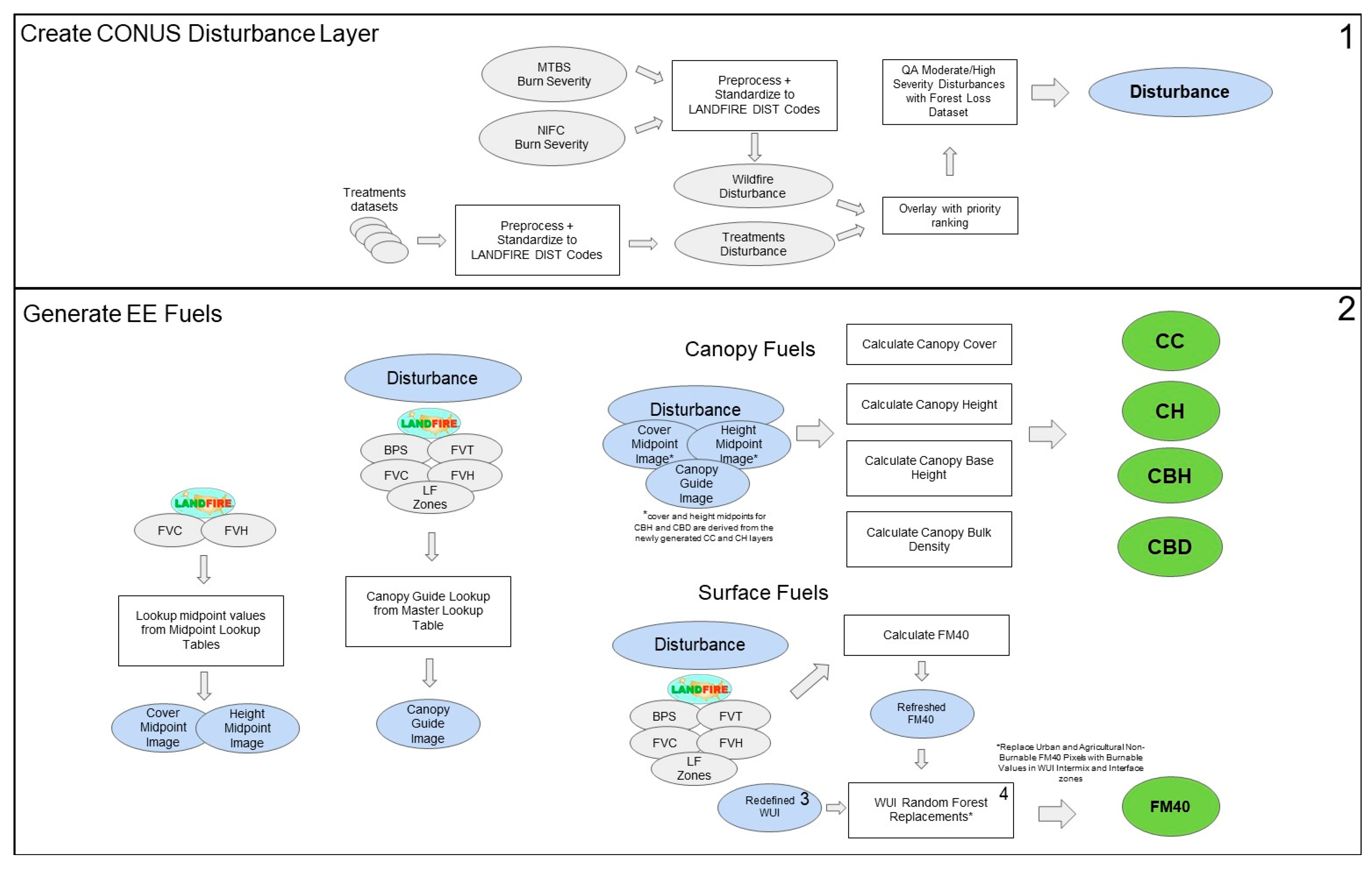
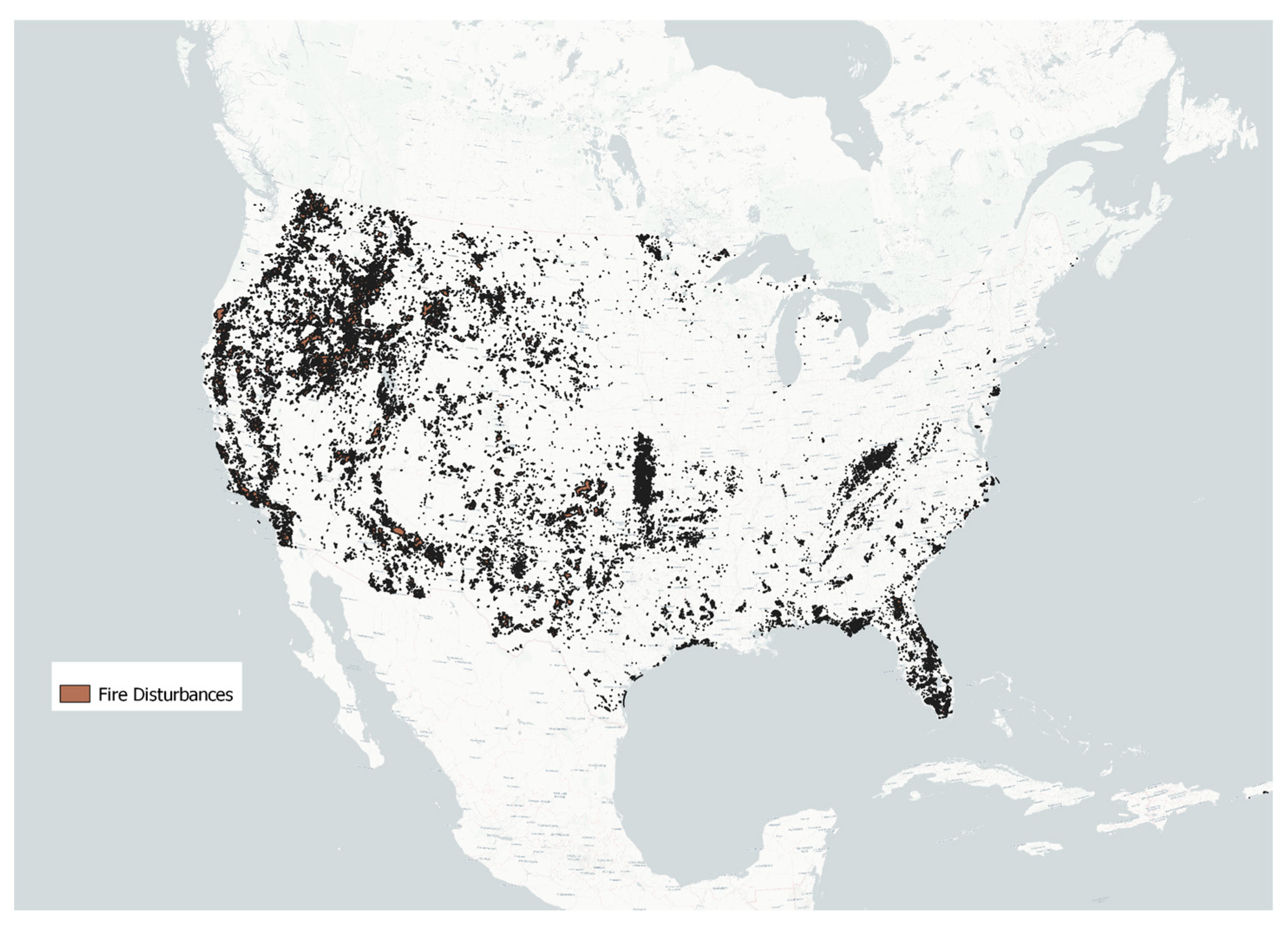
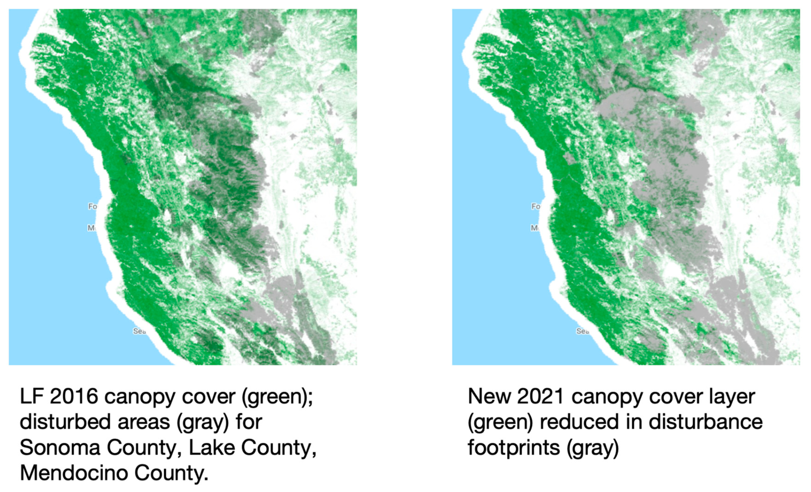

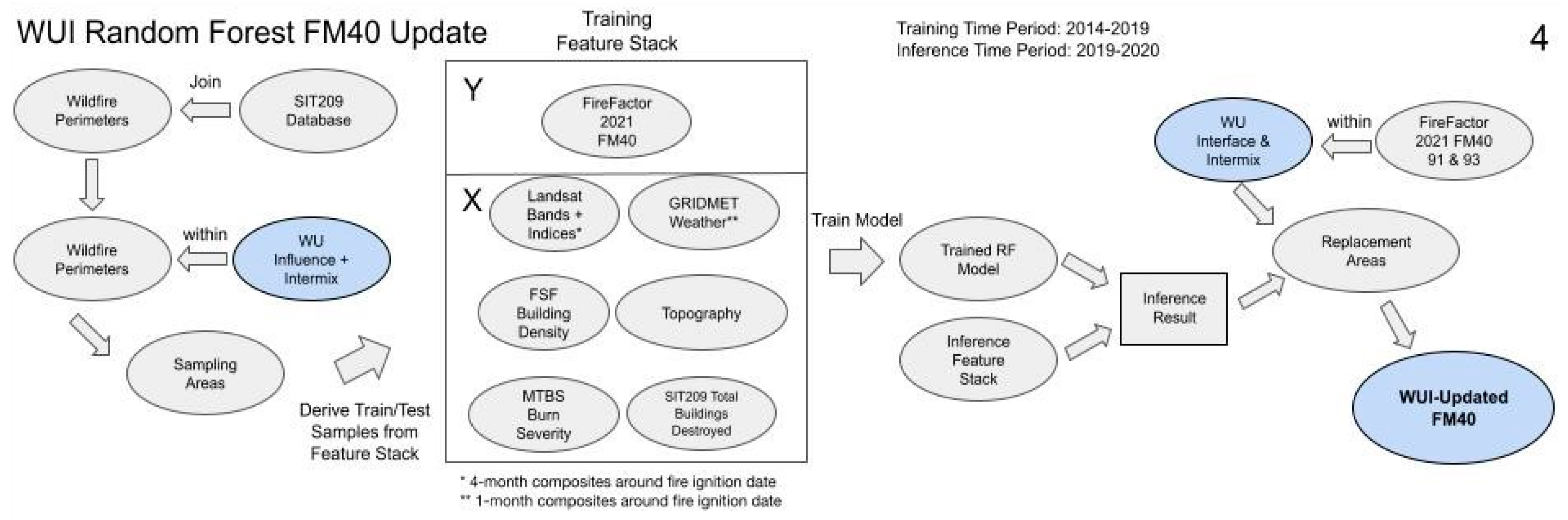

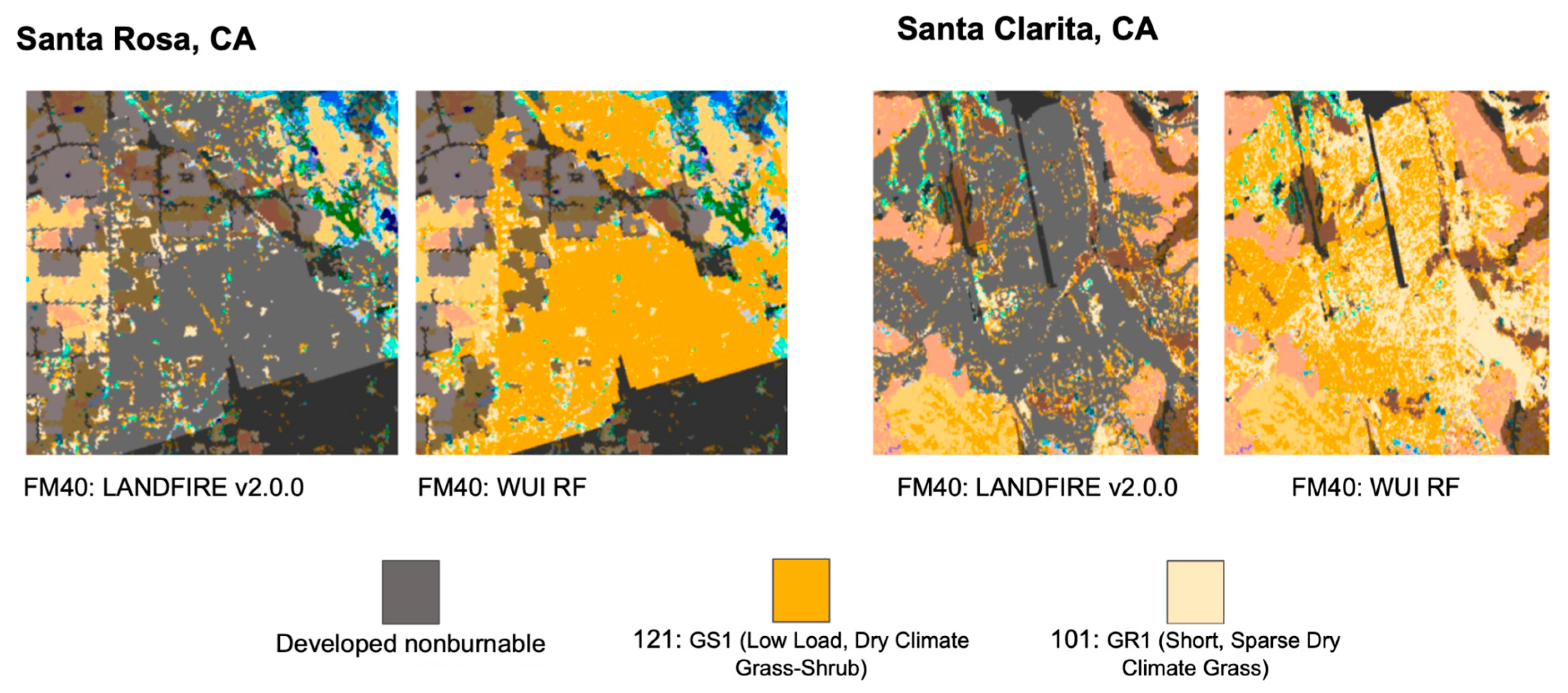
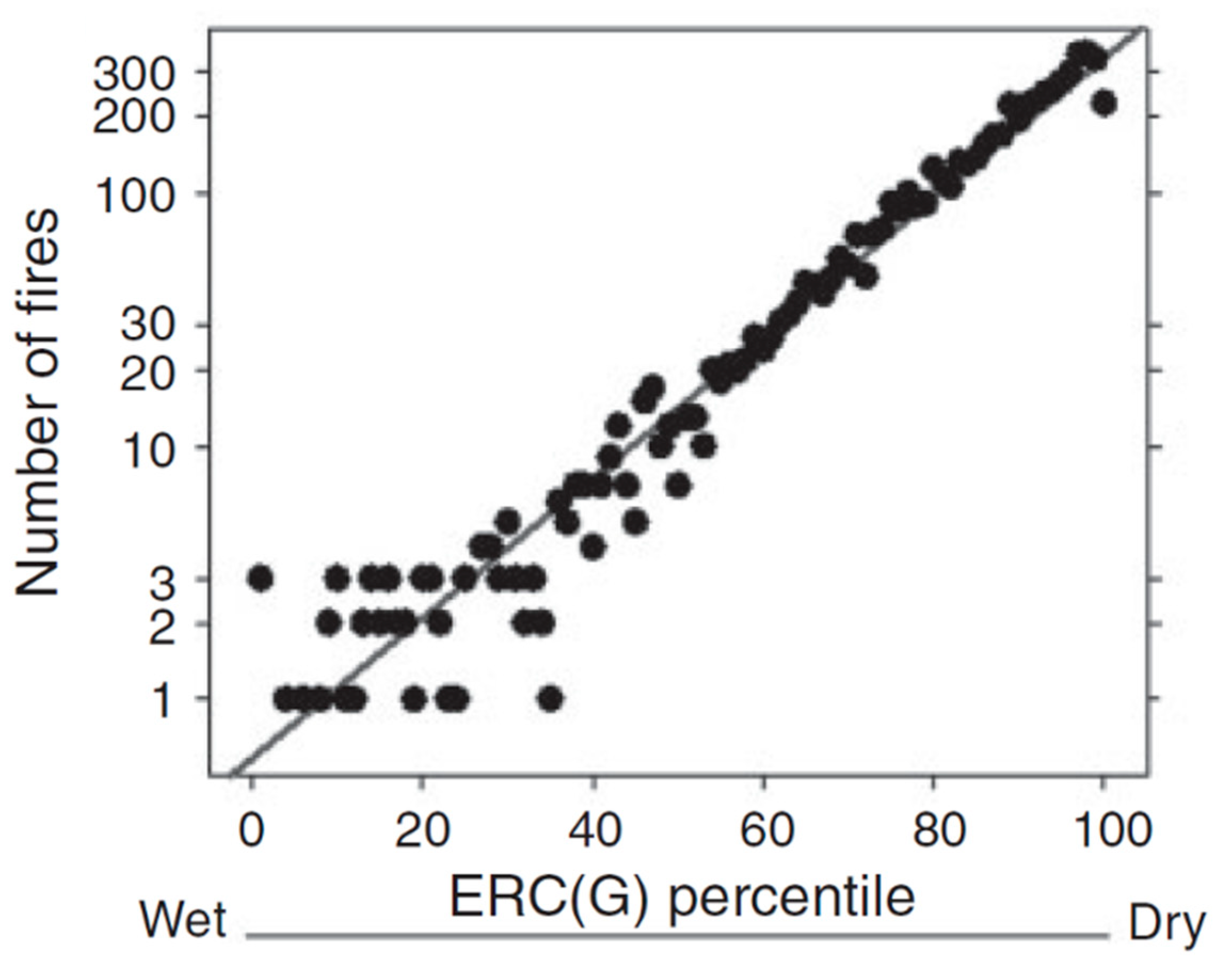
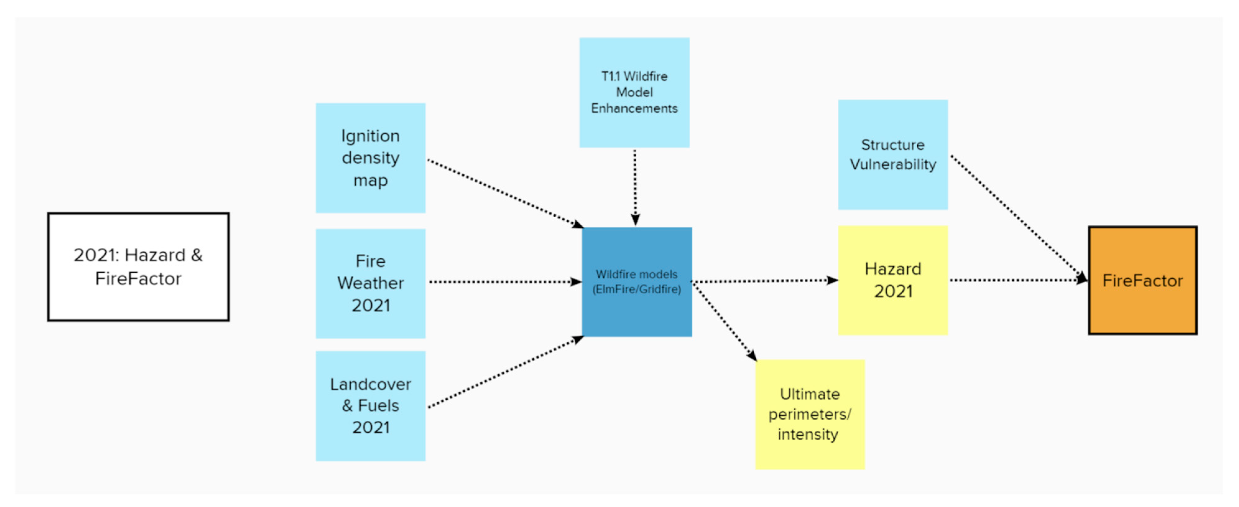

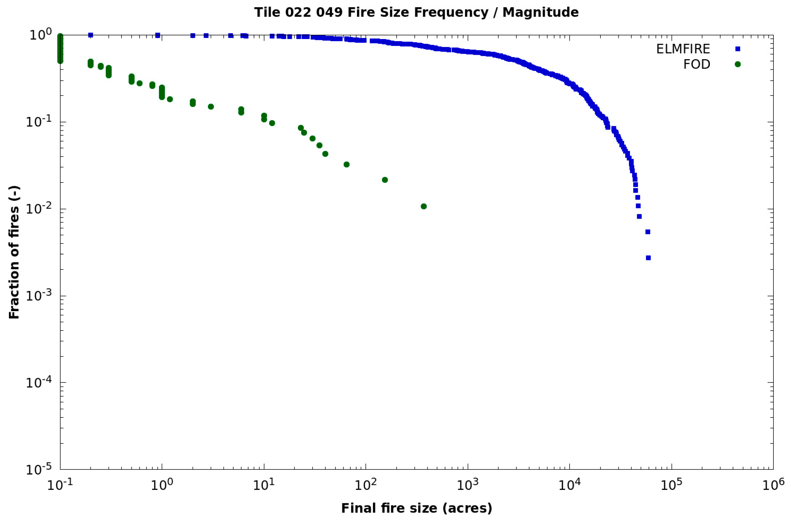


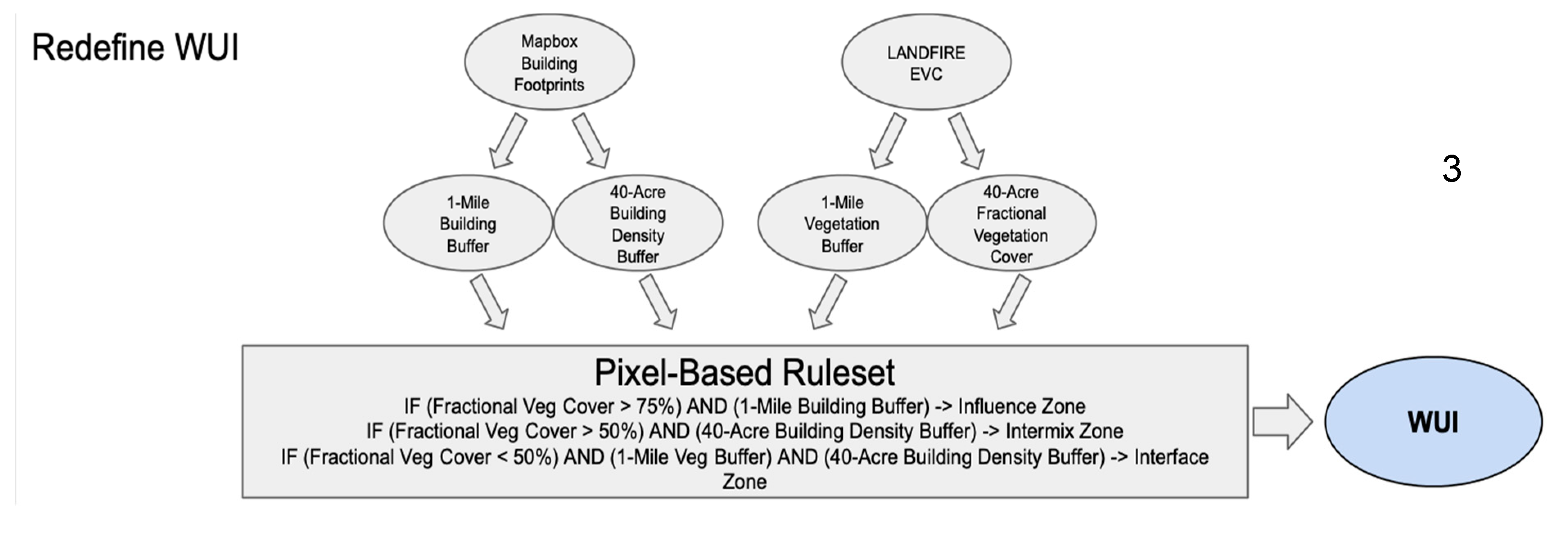
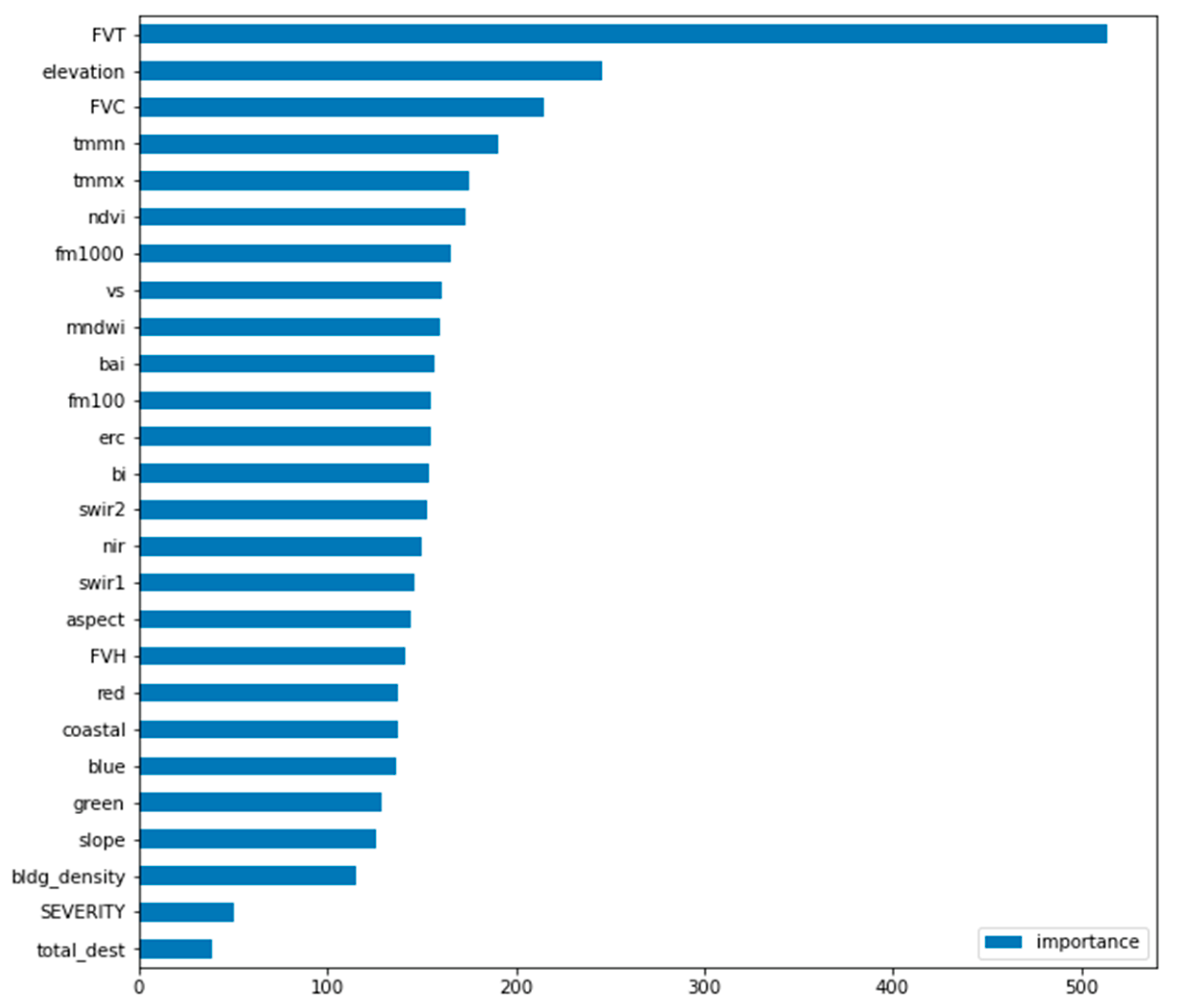
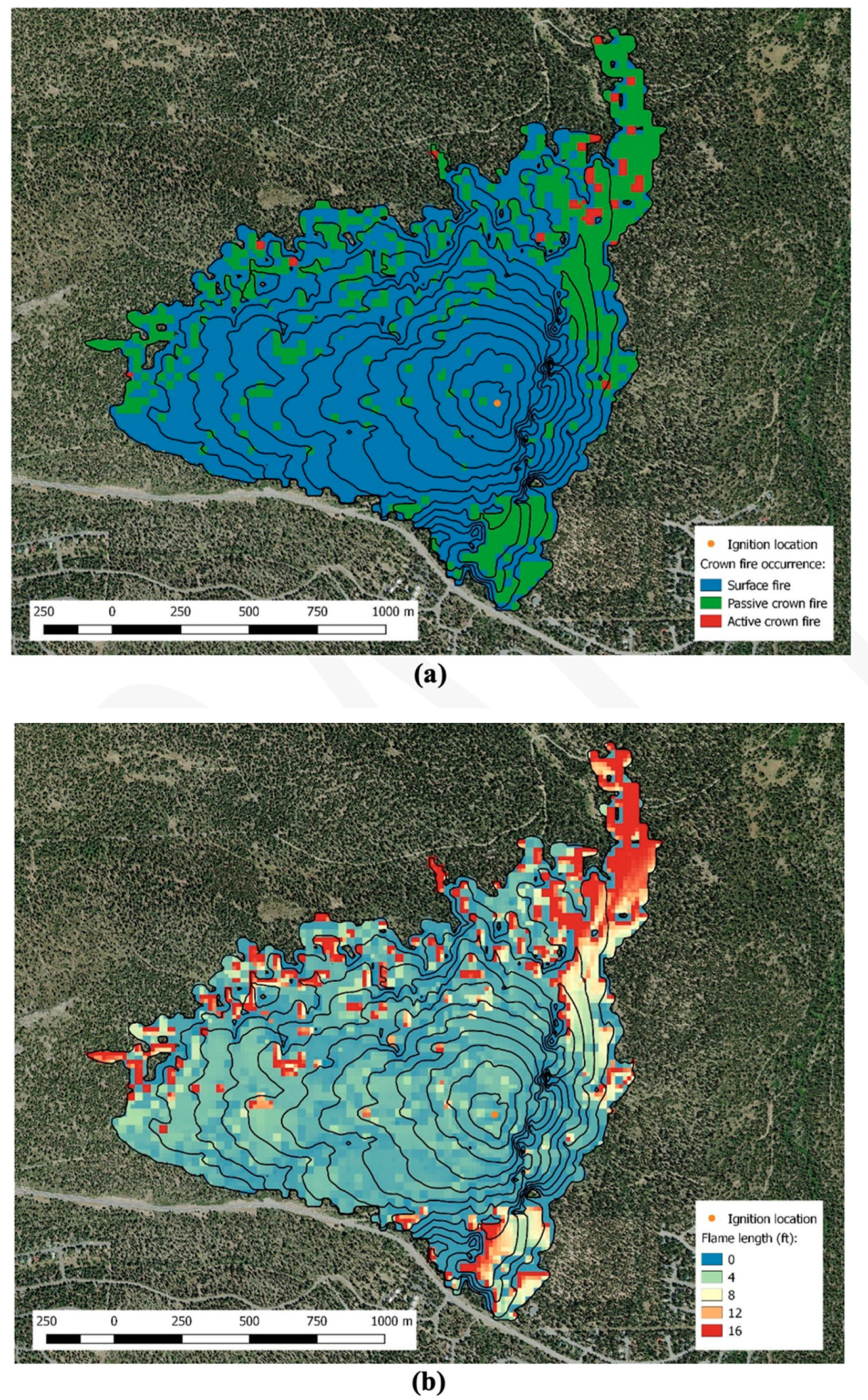
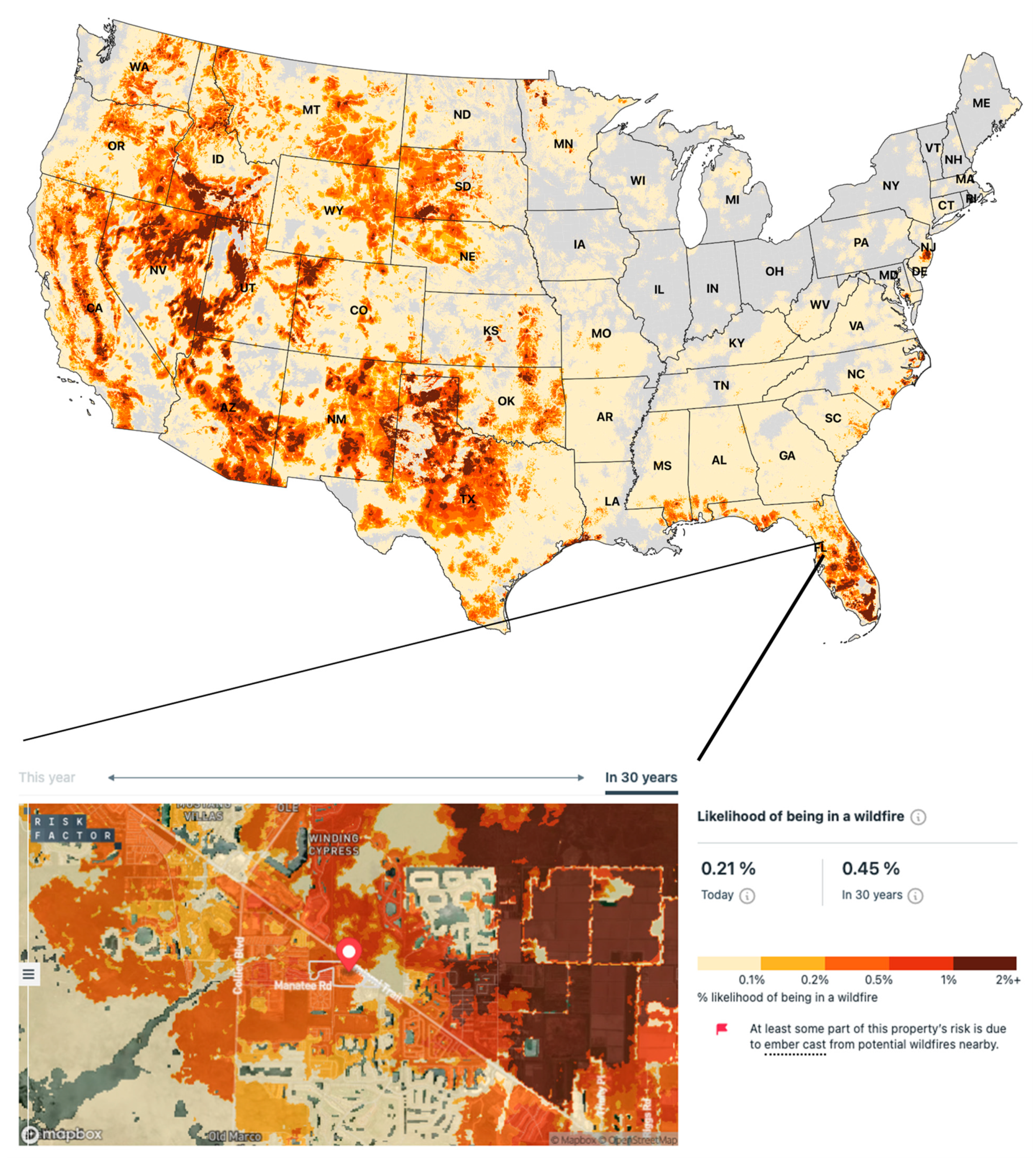
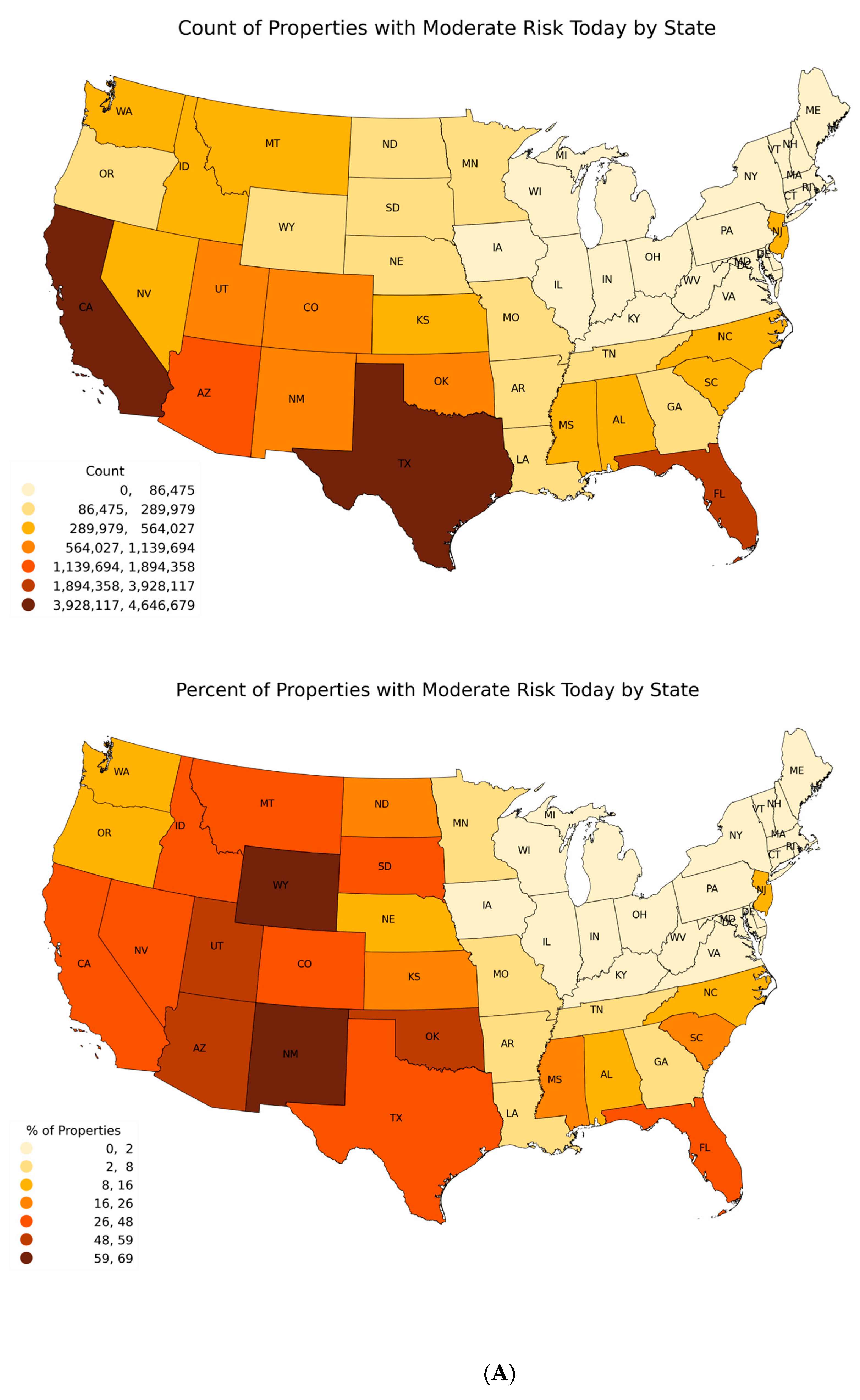
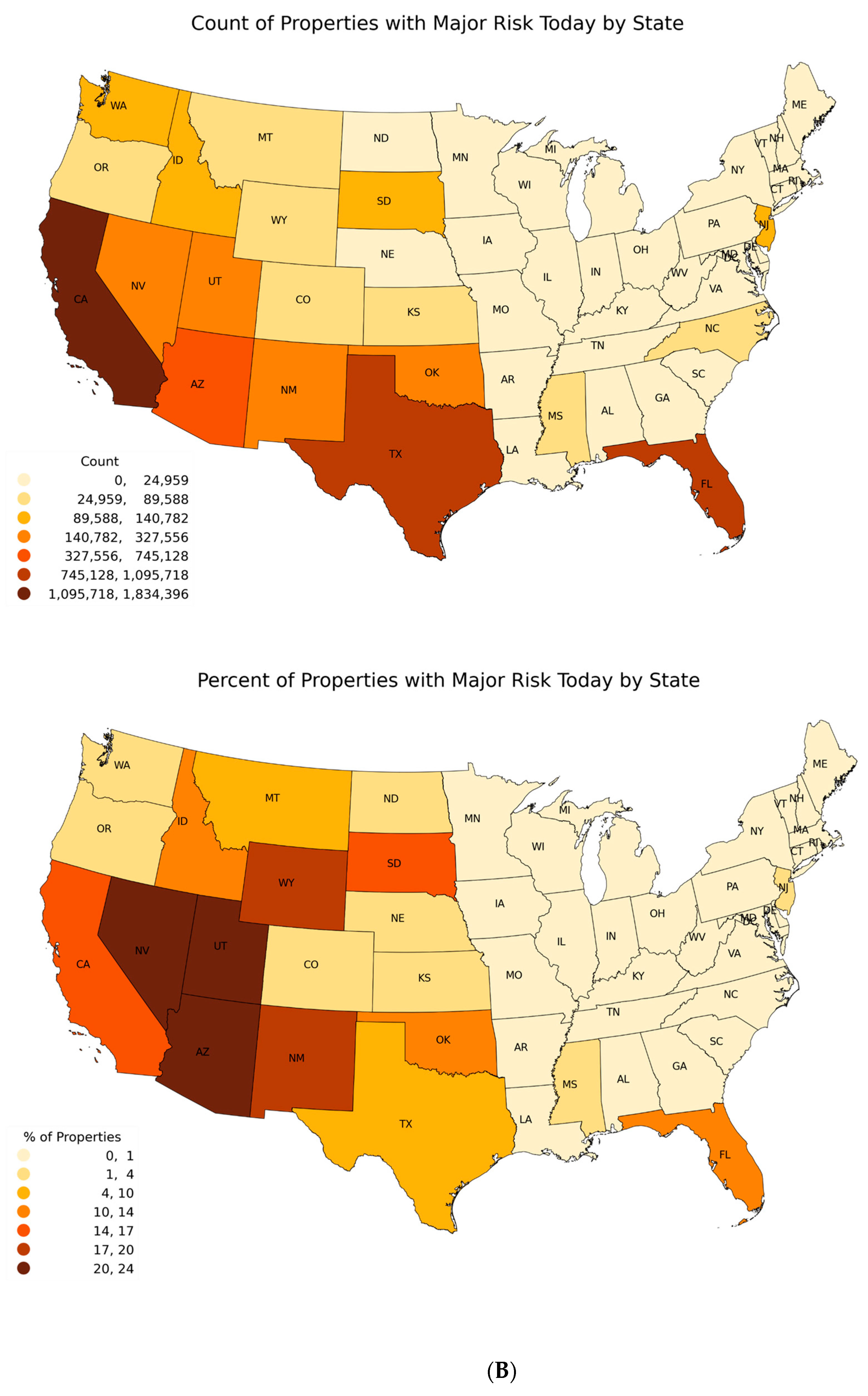
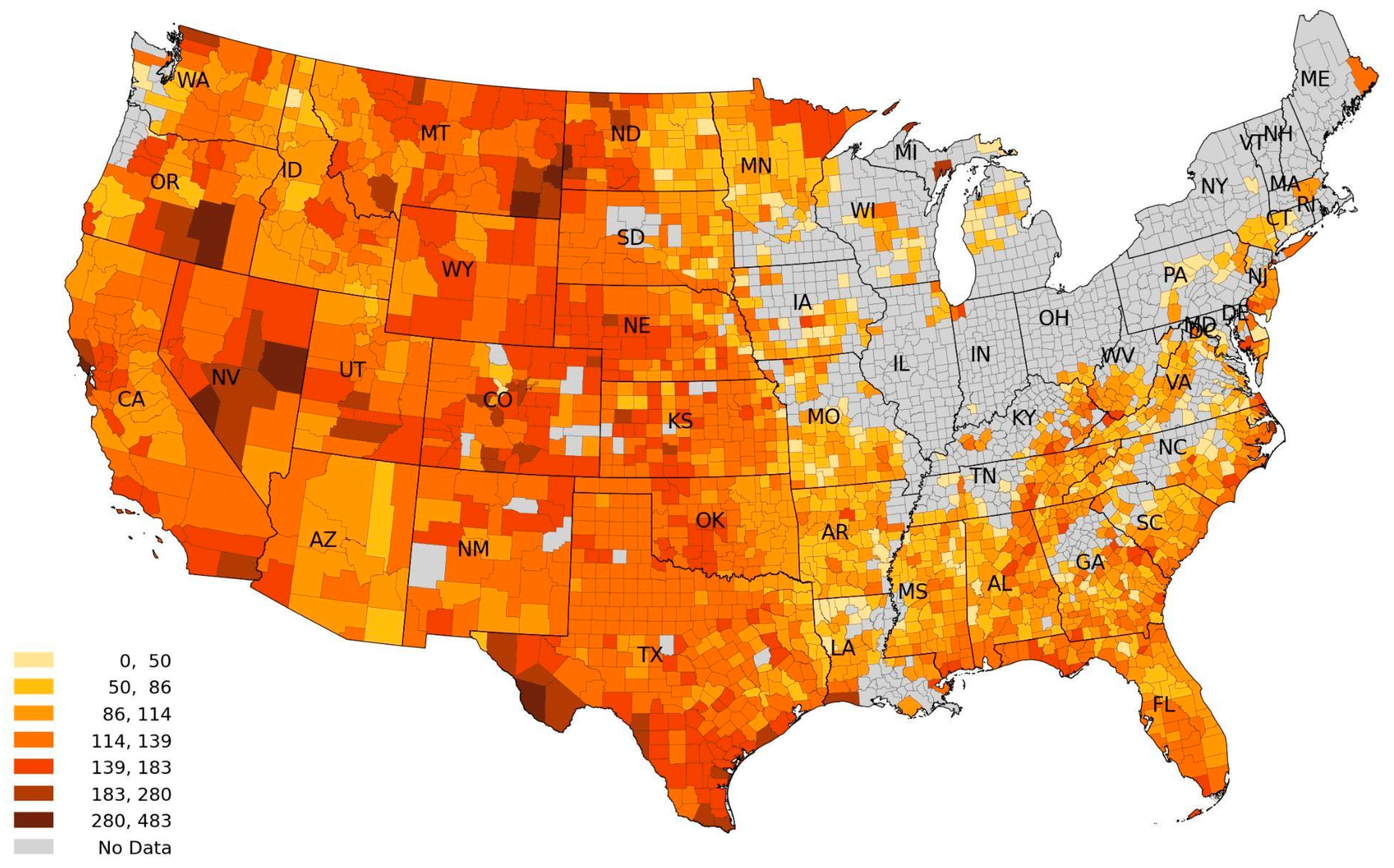