
Using Structure Location Data to Map the Wildland–Urban Interface in Montana, USA

 ,
,  , ,
, ,  , and
, and
Abstract
:1. Introduction
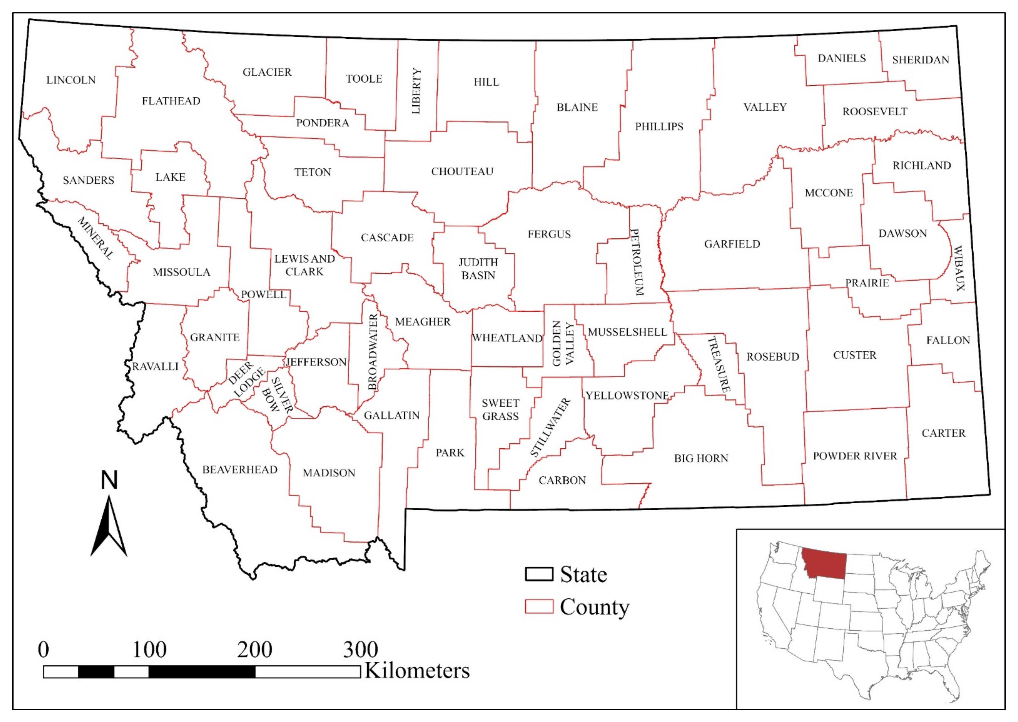
2. Study Area
3. Methods
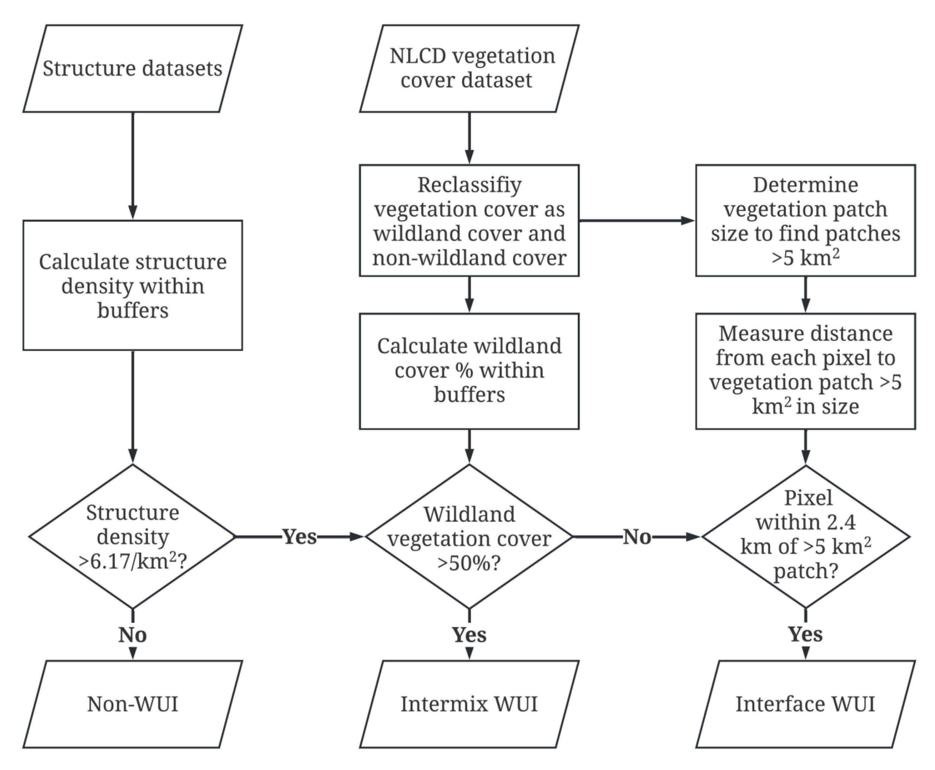
3.1. Mapping the WUI
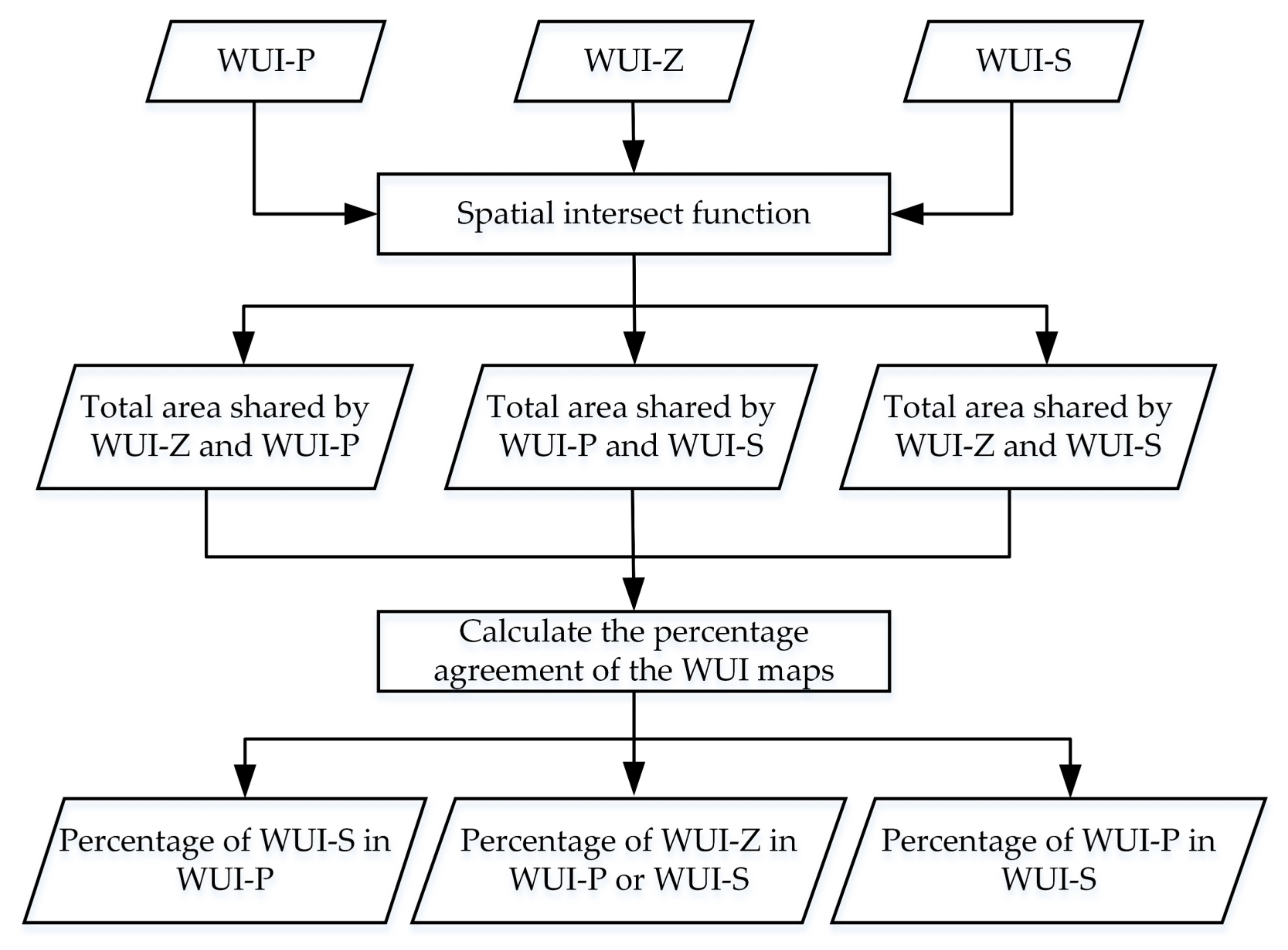
3.2. Map Comparison
3.3. Estimating WUI Population
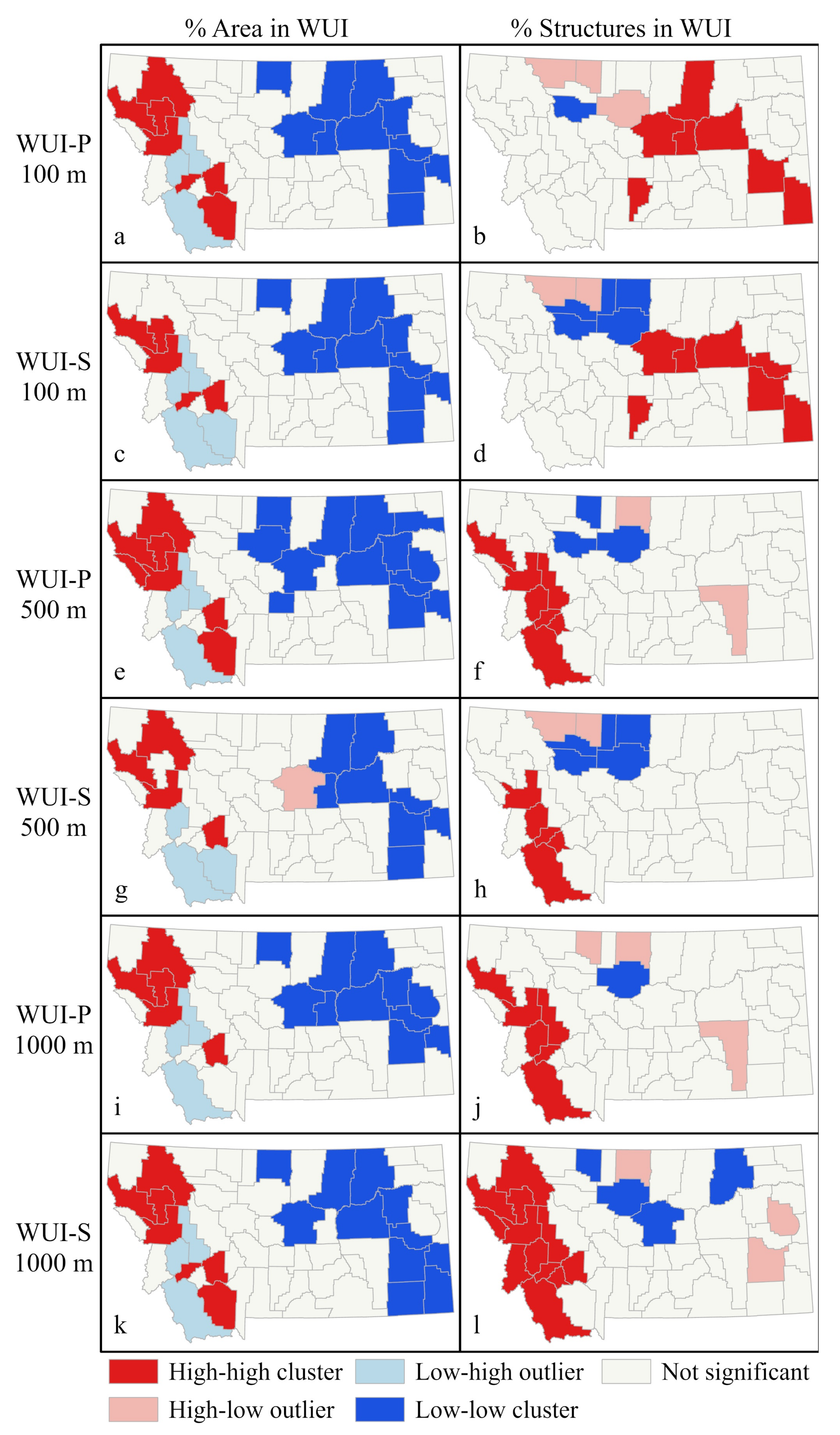
3.4. Spatial Analysis of WUI
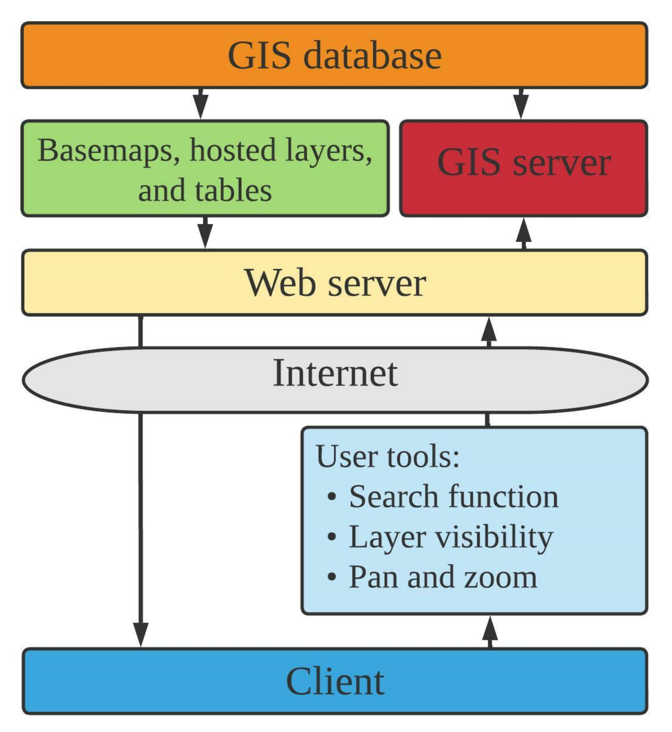
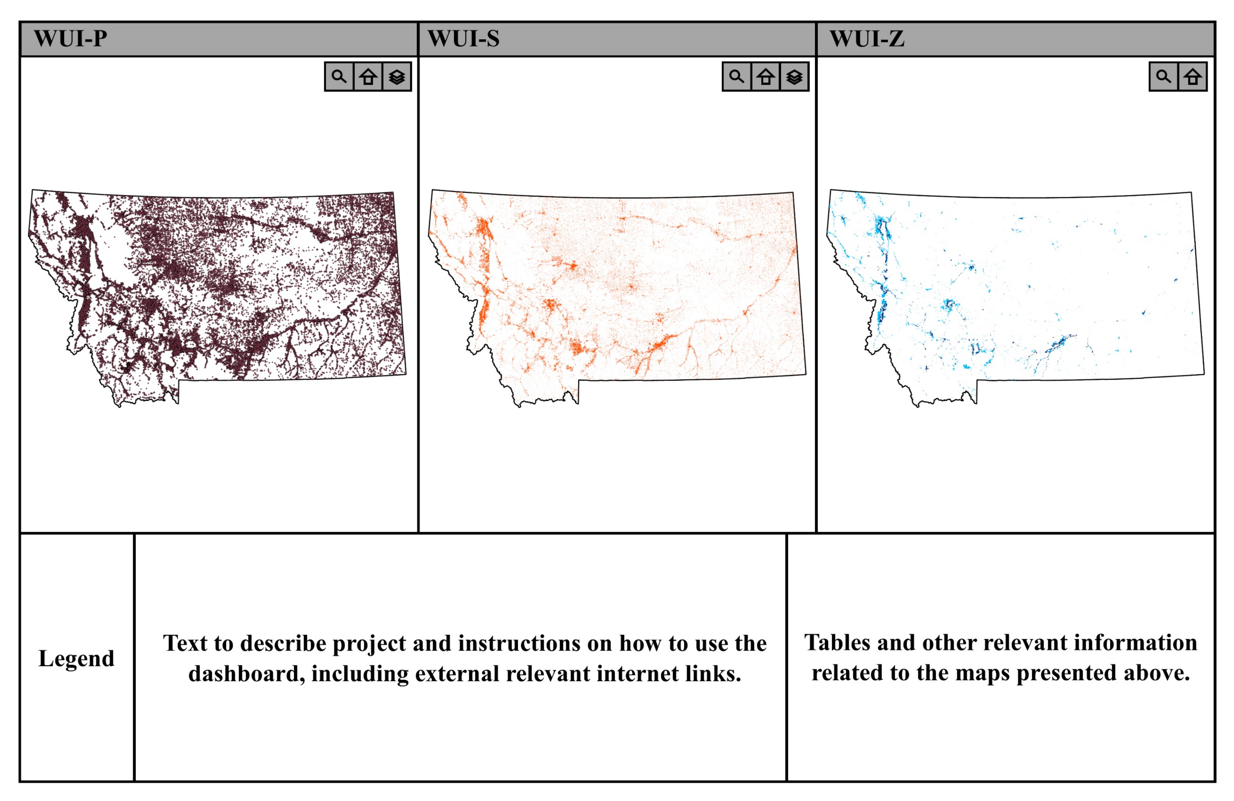
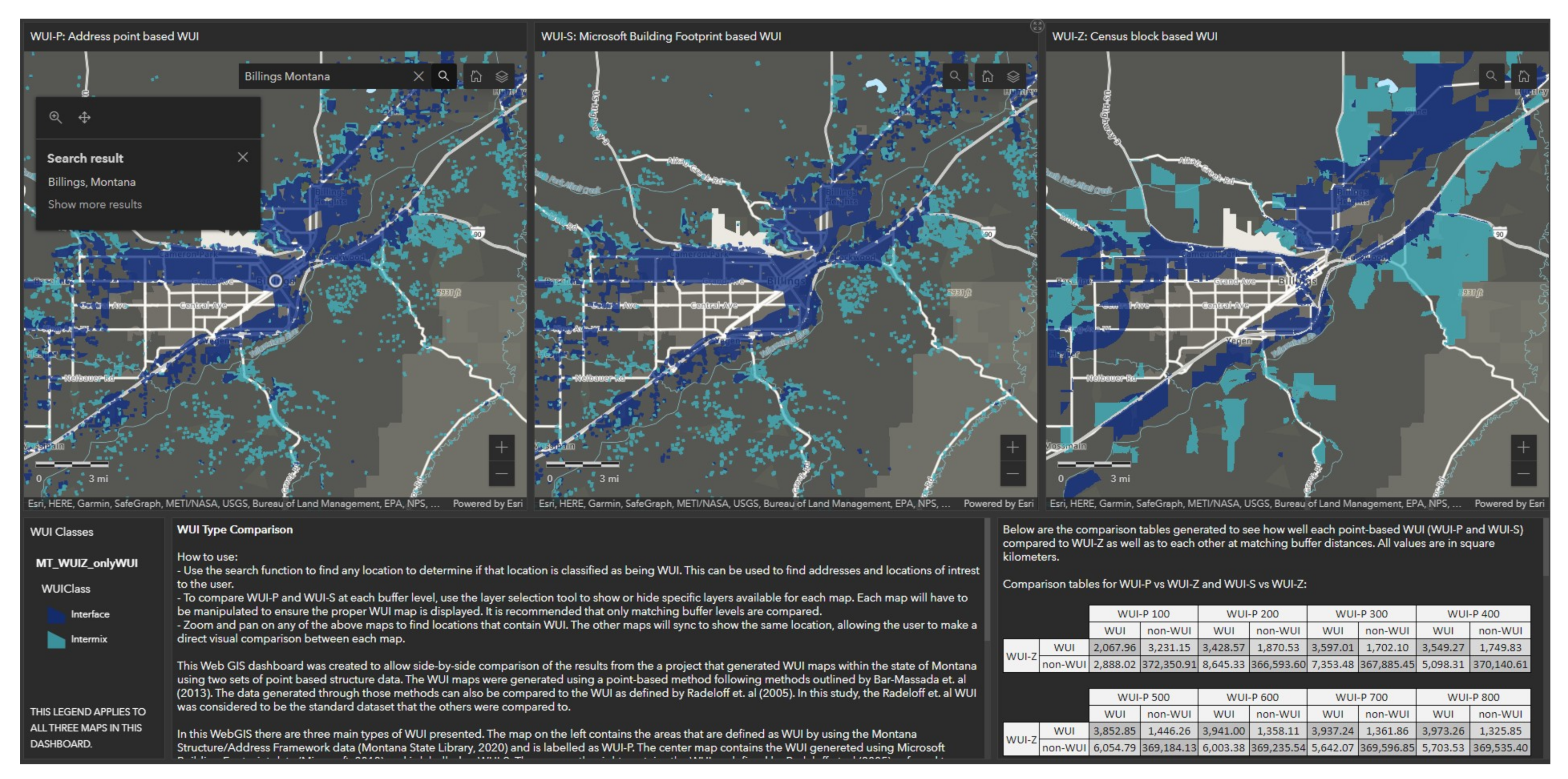
3.5. Web Mapping
4. Results
4.1. WUI Maps
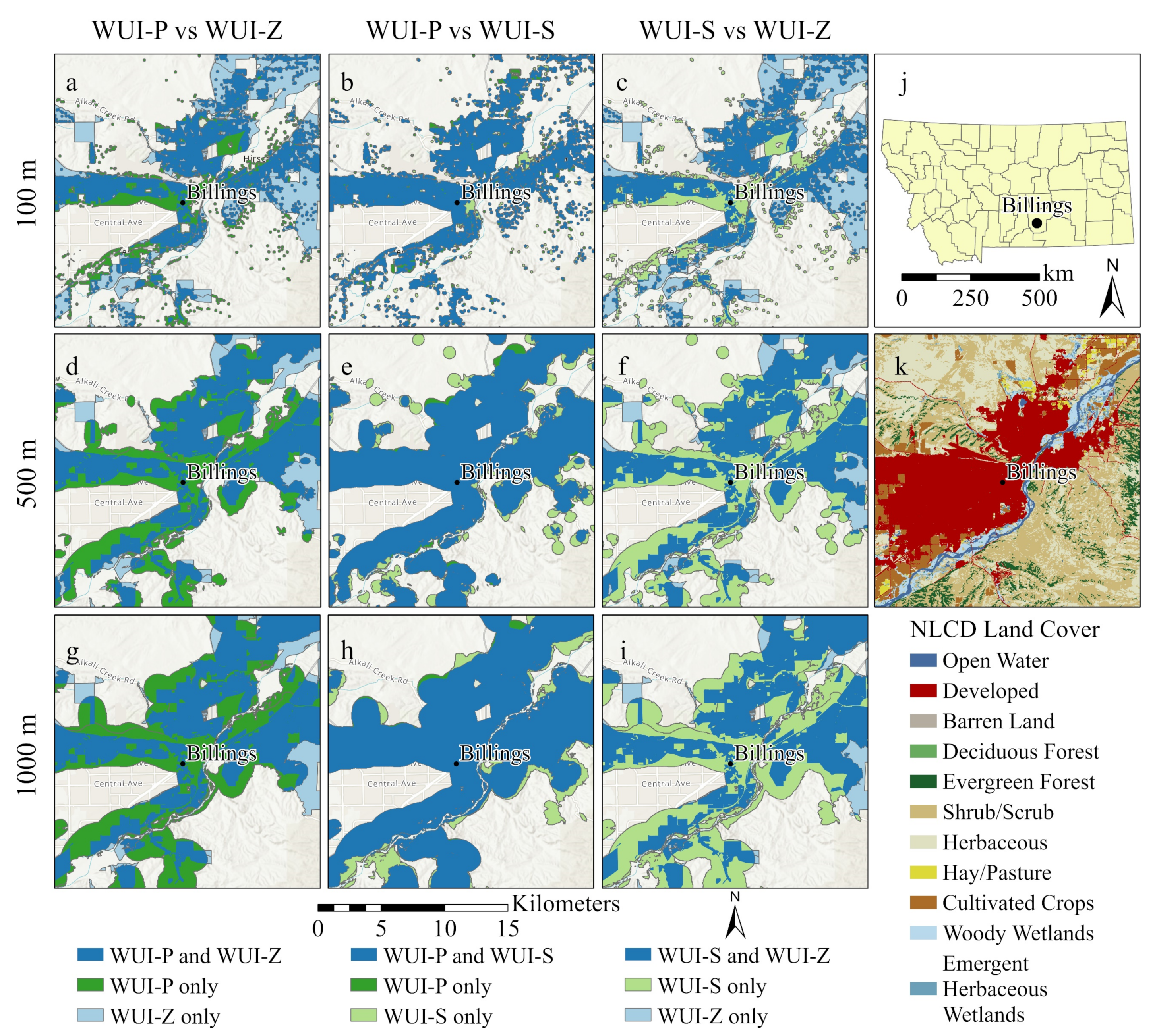
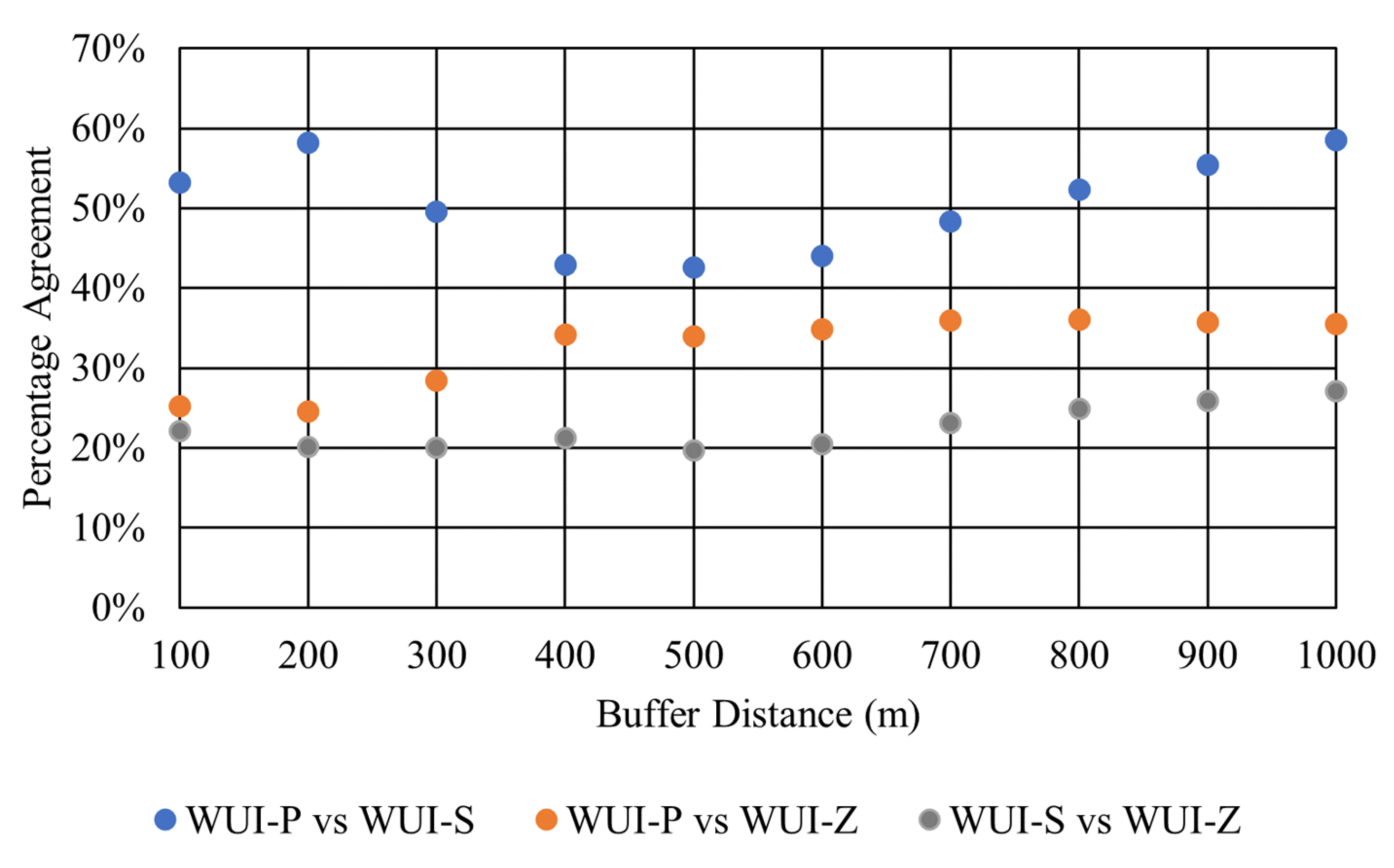
4.2. Map Comparison
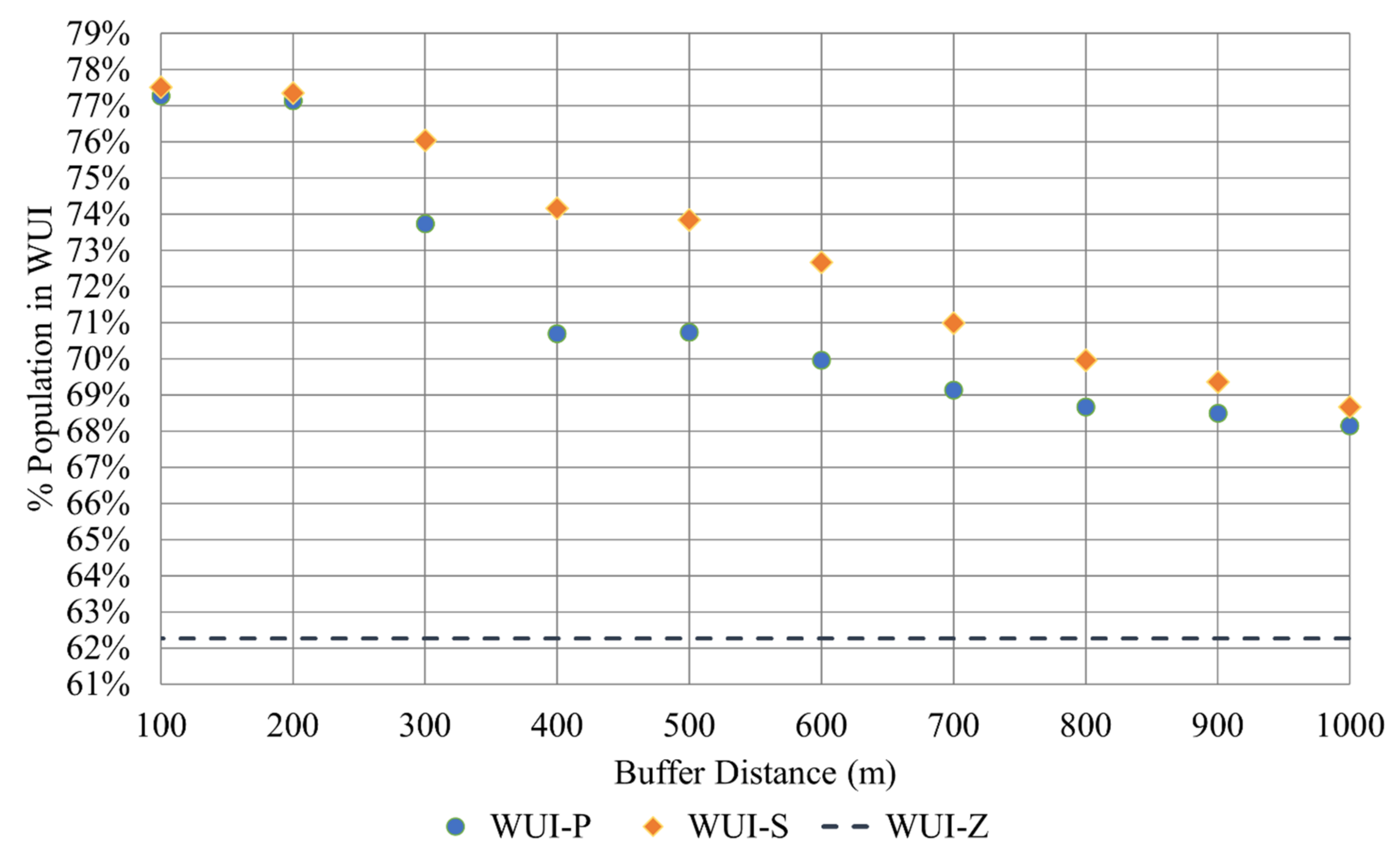
4.3. WUI Population Estimates
4.4. The Spatial Patterns of WUI
4.5. A Web GIS Application for Mapping the WUI
5. Discussion
6. Conclusions
Author Contributions
Funding
Institutional Review Board Statement
Informed Consent Statement
Data Availability Statement
Acknowledgments
Conflicts of Interest
Appendix A

| WUI-Z | WUI-P 100 | WUI-P 200 | WUI-P 300 | WUI-P 400 | WUI-P 500 | WUI-P 600 | WUI-P 700 | WUI-P 800 | WUI-P 900 | WUI-P 1000 | |
|---|---|---|---|---|---|---|---|---|---|---|---|
| WUI-Z | 5299.1 | 2068.0 | 3428.6 | 3597.0 | 3549.3 | 3852.8 | 3941.0 | 3937.2 | 3973.3 | 4026.5 | 4030.2 |
| WUI-S 100 | 2075.9 | 3870.8 | 5025.7 | 4100.6 | 3392.2 | 3426.6 | 3308.6 | 3161.4 | 3089.1 | 3063.4 | 3009.6 |
| WUI-S 200 | 3405.0 | 4402.2 | 9970.3 | 8069.6 | 6287.7 | 6490.7 | 6222.8 | 5858.1 | 5699.2 | 5653.8 | 5533.9 |
| WUI-S 300 | 3780.7 | 4283.7 | 9677.9 | 9375.1 | 7323.3 | 7630.1 | 7301.9 | 6850.3 | 6659.8 | 6606.7 | 6457.7 |
| WUI-S 400 | 3859.2 | 3983.2 | 8668.9 | 8783.4 | 7628.4 | 8048.8 | 7701.8 | 7226.2 | 7019.5 | 6952.6 | 6789.4 |
| WUI-S 500 | 4132.8 | 4009.0 | 8768.5 | 8926.3 | 7827.9 | 8898.8 | 8663.7 | 8131.2 | 7915.5 | 7859.8 | 7673.0 |
| WUI-S 600 | 4231.0 | 3865.0 | 8288.9 | 8587.1 | 7712.7 | 8874.5 | 9036.7 | 8584.8 | 8395.5 | 8353.9 | 8158.6 |
| WUI-S 700 | 4241.3 | 3648.9 | 7588.2 | 8008.9 | 7428.1 | 8594.9 | 8887.9 | 8744.3 | 8656.7 | 8647.4 | 8454.4 |
| WUI-S 800 | 4274.2 | 3526.0 | 7203.4 | 7652.5 | 7226.4 | 8389.8 | 8745.1 | 8708.5 | 8864.0 | 8959.9 | 8797.1 |
| WUI-S 900 | 4314.0 | 3460.5 | 7003.6 | 7447.0 | 7093.6 | 8253.5 | 8646.8 | 8655.4 | 8879.9 | 9181.0 | 9115.4 |
| WUI-S 1000 | 4316.6 | 3371.8 | 6746.0 | 7190.7 | 6915.8 | 8049.6 | 8464.8 | 8517.8 | 8777.2 | 9140.2 | 9244.9 |
| WUI-Z | WUI-S 100 | WUI-S 200 | WUI-S 300 | WUI-S 400 | WUI-S 500 | WUI-S 600 | WUI-S 700 | WUI-S 800 | WUI-S 900 | WUI-S 1000 | |
|---|---|---|---|---|---|---|---|---|---|---|---|
| WUI-Z | 100.0% | 22.1% | 20.1% | 20.0% | 21.2% | 19.6% | 20.4% | 23.1% | 24.9% | 25.8% | 27.1% |
| WUI-P 100 | 25.3% | 53.3% | 28.3% | 23.8% | 22.5% | 19.3% | 18.6% | 19.6% | 20.1% | 20.1% | 20.4% |
| WUI-P 200 | 24.6% | 38.0% | 58.2% | 49.0% | 43.0% | 37.8% | 35.4% | 34.9% | 34.3% | 33.7% | 33.3% |
| WUI-P 300 | 28.4% | 31.5% | 45.1% | 49.5% | 46.5% | 40.8% | 39.0% | 39.6% | 39.4% | 38.7% | 38.4% |
| WUI-P 400 | 34.1% | 29.7% | 36.2% | 39.2% | 43.0% | 37.8% | 37.5% | 40.2% | 41.2% | 41.1% | 41.5% |
| WUI-P 500 | 33.9% | 27.1% | 35.2% | 38.9% | 43.3% | 42.6% | 42.9% | 46.2% | 47.6% | 47.5% | 47.9% |
| WUI-P 600 | 34.9% | 25.8% | 33.2% | 36.5% | 40.6% | 40.9% | 44.0% | 48.5% | 50.5% | 50.8% | 51.5% |
| WUI-P 700 | 36.0% | 25.1% | 31.3% | 34.1% | 37.9% | 38.1% | 41.6% | 48.3% | 51.3% | 52.0% | 53.2% |
| WUI-P 800 | 36.1% | 24.2% | 30.0% | 32.7% | 36.2% | 36.6% | 40.1% | 47.3% | 52.4% | 53.8% | 55.4% |
| WUI-P 900 | 35.7% | 23.3% | 29.2% | 31.8% | 35.1% | 35.7% | 39.2% | 46.4% | 52.2% | 55.5% | 57.8% |
| WUI-P 1000 | 35.5% | 22.7% | 28.3% | 30.8% | 33.9% | 34.4% | 37.8% | 44.7% | 50.5% | 54.6% | 58.6% |
References
- Radeloff, V.C.; Helmers, D.P.; Kramer, H.A.; Mockrin, M.H.; Alexandre, P.M.; Bar-Massada, A.; Butsic, V.; Hawbaker, T.J.; Martinuzzi, S.; Syphard, A.D.; et al. Rapid growth of the US wildland-urban interface raises wildfire risk. Proc. Natl. Acad. Sci. USA 2018, 115, 3314–3319. [Google Scholar] [CrossRef]
- Theobald, D.M.; Romme, W.H. Expansion of the US wildland–urban interface. Landsc. Urban Plan. 2007, 83, 340–354. [Google Scholar] [CrossRef]
- Burke, M.; Driscoll, A.; Heft-Neal, S.; Xue, J.; Burney, J.; Wara, M. The changing risk and burden of wildfire in the United States. Proc. Natl. Acad. Sci. USA 2021, 118, e2011048118. [Google Scholar] [CrossRef] [PubMed]
- Glickman, D.; Babbitt, B. Urban wildland interface communities within the vicinity of federal lands that are at high risk from wildfire. Fed. Regist. 2001, 66, 751–777. [Google Scholar]
- Stewart, S.I.; Radeloff, V.C.; Hammer, R.B.; Hawbaker, T.J. Defining the Wildland-Urban Interface. J. For. 2007, 105, 201–207. [Google Scholar]
- Radeloff, V.C.; Hammer, R.B.; Stewart, S.I.; Fried, J.S.; Holcomb, S.S.; McKeefry, J.F. The wildland-urban interface in the United States. Ecol. Appl. 2005, 15, 799–805. [Google Scholar] [CrossRef]
- Stewart, S.I.; Wilmer, B.; Hammer, R.B.; Aplet, G.H.; Hawbaker, T.J.; Miller, C.; Radeloff, V.C. Wildland-Urban Interface Maps Vary with Purpose and Context. J. For. 2009, 107, 78–83. [Google Scholar]
- Johnston, L.M.; Flannigan, M.D. Mapping Canadian wildland fire interface areas. Int. J. Wildland Fire 2018, 27, 1–14. [Google Scholar] [CrossRef]
- Balch, J.K.; Bradley, B.A.; Abatzoglou, J.T.; Nagy, R.C.; Fusco, E.J.; Mahood, A.L. Human-started wildfires expand the fire niche across the United States. Proc. Natl. Acad. Sci. USA 2017, 114, 2946–2951. [Google Scholar] [CrossRef]
- Parisien, M.-A.; Miller, C.; Parks, S.A.; DeLancey, E.R.; Robinne, F.-N.; Flannigan, M.D. The spatially varying influence of humans on fire probability in North America. Environ. Res. Lett. 2016, 11, 075005. [Google Scholar] [CrossRef]
- Dennison, P.E.; Brewer, S.C.; Arnold, J.D.; Moritz, M.A. Large wildfire trends in the western United States, 1984–2011. Geophys. Res. Lett. 2014, 41, 2928–2933. [Google Scholar] [CrossRef]
- Holden, Z.A.; Swanson, A.; Luce Charles, H.; Jolly, W.M.; Maneta, M.; Oyler Jared, W.; Warren Dyer, A.; Parsons, R.; Affleck, D. Decreasing fire season precipitation increased recent western US forest wildfire activity. Proc. Natl. Acad. Sci. USA 2018, 115, E8349–E8357. [Google Scholar] [PubMed]
- Abatzoglou, J.T.; Williams, A.P. Impact of anthropogenic climate change on wildfire across western US forests. Proc. Natl. Acad. Sci. USA 2016, 113, 11770–11775. [Google Scholar] [CrossRef] [PubMed] [Green Version]
- Abatzoglou, J.T.; Juang, C.S.; Williams, A.P.; Kolden, C.A.; Westerling, A.L. Increasing Synchronous Fire Danger in Forests of the Western United States. Geophys. Res. Lett. 2021, 48, e2020GL091377. [Google Scholar]
- Miller, C.; Ager, A.A. A review of recent advances in risk analysis for wildfire management. Int. J. Wildland Fire 2013, 22, 1–14. [Google Scholar]
- Haynes, K.; Short, K.; Xanthopoulos, G.; Viegas, D.; Ribeiro, L.M.; Blanchi, R. Wildfires and WUI fire fatalities. In Encyclopedia of Wildfires and Wildland-Urban Interface (WUI) Fires; Manzello, S.L., Ed.; Springer: Cham, Switzerland, 2020; p. 16. [Google Scholar]
- Nagy, R.C.; Fusco, E.; Bradley, B.; Abatzoglou, J.T.; Balch, J. Human-Related Ignitions Increase the Number of Large Wildfires across U.S. Ecoregions. Fire 2018, 1, 4. [Google Scholar] [CrossRef]
- Alexandre, P.M.; Stewart, S.I.; Keuler, N.S.; Clayton, M.K.; Mockrin, M.H.; Bar-Massada, A.; Syphard, A.D.; Radeloff, V.C. Factors related to building loss due to wildfires in the conterminous United States. Ecol. Appl. 2016, 26, 2323–2338. [Google Scholar] [PubMed]
- Alexandre, P.M.; Stewart, S.I.; Mockrin, M.H.; Keuler, N.S.; Syphard, A.D.; Bar-Massada, A.; Clayton, M.K.; Radeloff, V.C. The relative impacts of vegetation, topography and spatial arrangement on building loss to wildfires in case studies of California and Colorado. Landsc. Ecol. 2016, 31, 415–430. [Google Scholar]
- Syphard, A.D.; Keeley, J.E. Factors associated with structure loss in the 2013–2018 California wildfires. Fire 2019, 2, 49. [Google Scholar] [CrossRef] [Green Version]
- Syphard, A.D.; Keeley, J.E.; Massada, A.B.; Brennan, T.J.; Radeloff, V.C. Housing arrangement and location determine the likelihood of housing loss due to wildfire. PLoS ONE 2012, 7, e33954. [Google Scholar]
- Ager, A.A.; Palaiologou, P.; Evers, C.R.; Day, M.A.; Ringo, C.; Short, K. Wildfire exposure to the wildland urban interface in the western US. Appl. Geogr. 2019, 111, 102059. [Google Scholar]
- Caggiano, M.D.; Hawbaker, T.J.; Gannon, B.M.; Hoffman, C.M. Building Loss in WUI Disasters: Evaluating the Core Components of the Wildland–Urban Interface Definition. Fire 2020, 3, 73. [Google Scholar]
- Kramer, H.A.; Mockrin, M.H.; Alexandre, P.M.; Radeloff, V.C. High wildfire damage in interface communities in California. Int. J. Wildland Fire 2019, 28, 641–650. [Google Scholar]
- Kramer, H.A.; Mockrin, M.H.; Alexandre, P.M.; Stewart, S.I.; Radeloff, V.C. Where wildfires destroy buildings in the US relative to the wildland–urban interface and national fire outreach programs. Int. J. Wildland Fire 2018, 27, 329–341. [Google Scholar]
- Haight, R.G.; Cleland, D.T.; Hammer, R.B.; Radeloff, V.C.; Rupp, T.S. Assessing fire risk in the wildland-urban interface. J. For. 2004, 102, 41–48. [Google Scholar]
- Moritz, M.A.; Batllori, E.; Bradstock, R.A.; Gill, A.M.; Handmer, J.; Hessburg, P.F.; Leonard, J.; McCaffrey, S.; Odion, D.C.; Schoennagel, T.; et al. Learning to coexist with wildfire. Nature 2014, 515, 58–66. [Google Scholar]
- Bar-Massada, A.; Stewart, S.I.; Hammer, R.B.; Mockrin, M.H.; Radeloff, V.C. Using structure locations as a basis for mapping the wildland urban interface. J. Environ. Manag. 2013, 128, 540–547. [Google Scholar]
- Platt, R.V. The wildland–urban interface: Evaluating the definition effect. J. For. 2010, 108, 9–15. [Google Scholar]
- Argañaraz, J.P.; Radeloff, V.C.; Bar-Massada, A.; Gavier-Pizarro, G.I.; Scavuzzo, C.M.; Bellis, L.M. Assessing wildfire exposure in the Wildland-Urban Interface area of the mountains of central Argentina. J. Environ. Manag. 2017, 196, 499–510. [Google Scholar]
- Conedera, M.; Tonini, M.; Oleggini, L.; Vega Orozco, C.; Leuenberger, M.; Pezzatti, G.B. Geospatial approach for defining the Wildland-Urban Interface in the Alpine environment. Comput. Environ. Urban Syst. 2015, 52, 10–20. [Google Scholar]
- Lampin-Maillet, C.; Jappiot, M.; Long, M.; Bouillon, C.; Morge, D.; Ferrier, J.-P. Mapping wildland-urban interfaces at large scales integrating housing density and vegetation aggregation for fire prevention in the South of France. J. Environ. Manag. 2010, 91, 732–741. [Google Scholar]
- Miranda, A.; Carrasco, J.; González, M.; Pais, C.; Lara, A.; Altamirano, A.; Weintraub, A.; Syphard, A.D. Evidence-based mapping of the wildland-urban interface to better identify human communities threatened by wildfires. Environ. Res. Lett. 2020, 15, 094069. [Google Scholar]
- Calkin, D.E.; Rieck, J.D.; Hyde, K.D.; Kaiden, J.D. Built structure identification in wildland fire decision support. Int. J. Wildland Fire 2011, 20, 78–90. [Google Scholar]
- Li, D.; Cova, T.J.; Dennison, P.E.; Wan, N.; Nguyen, Q.C.; Siebeneck, L.K. Why do we need a national address point database to improve wildfire public safety in the U.S.? Int. J. Disaster Risk Reduct. 2019, 39, 101237. [Google Scholar]
- Microsoft. US Building Footprints. Available online: https://github.com/microsoft/USBuildingFootprints (accessed on 23 March 2021).
- Huang, X.; Wang, C.; Li, Z.; Ning, H. A 100 m population grid in the CONUS by disaggregating census data with open-source microsoft building footprints. Big Earth Data 2021, 5, 1–22. [Google Scholar]
- Huang, X.; Wang, C. Estimates of exposure to the 100-year floods in the conterminous United States using national building footprints. Int. J. Disaster Risk Reduct. 2020, 50, 101731. [Google Scholar]
- Carlson, A.R.; Helmers, D.P.; Hawbaker, T.J.; Mockrin, M.H.; Radeloff, V.C. The wildland-urban interface in the United States based on 125 million building locations. Ecol. Appl. 2022, 32, e2597. [Google Scholar]
- Bar-Massada, A. A Comparative Analysis of Two Major Approaches for Mapping the Wildland-Urban Interface: A Case Study in California. Land 2021, 10, 679. [Google Scholar]
- Li, S.; Dao, V.; Kumar, M.; Nguyen, P.; Banerjee, T. Mapping the wildland-urban interface in California using remote sensing data. Sci. Rep. 2022, 12, 5789. [Google Scholar]
- Whitlock, C.; Cross, W.; Maxwell, B.; Silverman, N.; Wade, A. Montana Climate Assessment; Montana State University: Bozeman, MT, USA, 2017; p. 18. [Google Scholar]
- Adams, A.; Byron, R.; Maxwell, B.; Higgins, S.; Eggers, M.; Byron, L.; Whitlock, C. Climate Change and Human Health in Montana: A Special Report of the Montana Climate Assessment; Montana State University: Bozeman, MT, USA, 2021; p. 14. [Google Scholar]
- Radeloff, V.C.; Mockrin, M.H.; Helmers, D.P.; Mapping Change in the Wildland Urban Interface (WUI) 1990–2010. State Summary Statistics June 2018. Available online: http://silvis.forest.wisc.edu/GeoData/WUI_cp12/WUI_change_1990_2010_State_Stats_Report.pdf (accessed on 4 April 2021).
- U.S. Census Bureau. Available online: https://www.census.gov/quickfacts/MT (accessed on 15 July 2022).
- Tapp, A.F. Areal interpolation and dasymetric mapping methods using local ancillary data sources. Cartogr. Geogr. Inf. Sci. 2010, 37, 215–228. [Google Scholar]
- Zandbergen, P.A. Dasymetric mapping using high resolution address point datasets. Trans. GIS 2011, 15, 5–27. [Google Scholar]
- Anselin, L. Local indicators of spatial association—LISA. Geogr. Anal. 1995, 27, 93–115. [Google Scholar]
- Bolstad, P. GIS Fundamentals: A First Text on Geographic Information Systems, 6th ed.; Eider Press: White Bear Lake, MN, USA, 2019. [Google Scholar]
- Harris, R. Quantitative Geography: The Basics; Sage: London, UK, 2016. [Google Scholar]
- Environmental Systems Research Institute. ArcGIS Online. Available online: https://www.arcgis.com (accessed on 23 March 2021).
- Fu, P.; Sun, J. Web GIS: Principles and Applications; ESRI Press: Redlands, CA, USA, 2011. [Google Scholar]
- Sehra, S.S.; Singh, J.; Rai, H.S. A Systematic Study of OpenStreetMap Data Quality Assessment. In Proceedings of the 2014 11th International Conference on Information Technology: New Generations, Las Vegas, NV, USA, 7–9 April 2014; pp. 377–381. [Google Scholar]
- Montana DNRC. Guidelines for Development within the Wildland-Urban Interface. 2009. Available online: http://dnrc.mt.gov/divisions/forestry/docs/fire-and-aviation/prevention/guidelinesfinal.pdf (accessed on 24 March 2021).
| Data | Data Source | Date | Format |
|---|---|---|---|
| Microsoft building footprint data | Microsoft | 2018 | Vector (polygon) |
| Montana structure/address framework | Montana State Library Geographic Information Services | 2020 | Vector (point) |
| Vegetation cover data (NLCD) | U.S. Geological Survey | 2016 | Raster |
| Montana state boundary | Montana State Library Geographic Information Services | 2020 | Vector (polygon) |
| Buffer Distance (m) | Intermix WUI-P | Interface WUI-P | WUI-P | Intermix WUI-S | Interface WUI-S | WUI-S |
|---|---|---|---|---|---|---|
| 100 | 3403.18 | 1552.80 | 4955.98 | 4201.29 | 1981.58 | 6182.88 |
| 200 | 8686.18 | 3387.73 | 12,073.90 | 10,590.12 | 4434.30 | 15,024.43 |
| 300 | 7777.51 | 3172.98 | 10,950.48 | 11,904.26 | 5448.97 | 17,353.23 |
| 400 | 6139.58 | 2508.00 | 8647.58 | 11,151.68 | 5584.64 | 16,736.32 |
| 500 | 7139.12 | 2768.52 | 9907.64 | 13,259.49 | 6618.96 | 19,878.45 |
| 600 | 7193.79 | 2750.59 | 9944.38 | 13,031.34 | 6603.06 | 19,634.40 |
| 700 | 6923.42 | 2655.90 | 9579.32 | 11,429.46 | 5842.45 | 17,271.91 |
| 800 | 7018.06 | 2658.73 | 9676.79 | 10,751.28 | 5365.80 | 16,117.08 |
| 900 | 7286.63 | 2728.69 | 10,015.32 | 10,526.75 | 5191.54 | 15,718.29 |
| 1000 | 7338.08 | 2745.20 | 10,083.28 | 10,090.48 | 4854.59 | 14,945.07 |
| Buffer Distance (m) | Intermix WUI-P | Interface WUI-P | WUI-P | Intermix WUI-S | Interface WUI-S | WUI-S |
|---|---|---|---|---|---|---|
| 100 | 193,205 | 333,031 | 526,236 | 293,055 | 348,807 | 641,862 |
| 200 | 194,536 | 330,912 | 525,448 | 286,643 | 353,281 | 639,924 |
| 300 | 178,304 | 320,778 | 499,082 | 270,657 | 348,779 | 619,436 |
| 400 | 164,343 | 309,183 | 473,526 | 251,476 | 338,938 | 590,414 |
| 500 | 169,876 | 302,770 | 472,646 | 250,686 | 332,990 | 583,676 |
| 600 | 169,342 | 297,328 | 466,670 | 239,243 | 323,569 | 562,812 |
| 700 | 168,044 | 291,569 | 459,613 | 222,348 | 310,722 | 533,070 |
| 800 | 172,147 | 283,491 | 455,638 | 215,752 | 298,227 | 513,979 |
| 900 | 175,652 | 278,220 | 453,872 | 212,330 | 290,240 | 502,570 |
| 1000 | 178,112 | 272,701 | 450,813 | 209,434 | 281,788 | 491,222 |
| WUI Type | Buffer Distance (m) | Non-WUI Population (2010) | Intermix-WUI Population (2010) | Interface-WUI Population (2010) | Total Population (2010) | Percentage Population in WUI (2010) |
|---|---|---|---|---|---|---|
| WUI-Z | NA | 373,358 | 155,175 | 460,882 | 989,415 | 62.26% |
| WUI-P | 100 | 224,904 | 231,378 | 533,133 | 989,415 | 77.27% |
| 200 | 226,189 | 232,753 | 530,472 | 989,415 | 77.14% | |
| 300 | 259,835 | 213,634 | 515,946 | 989,415 | 73.74% | |
| 400 | 289,931 | 198,440 | 501,044 | 989,415 | 70.70% | |
| 500 | 289,560 | 206,089 | 493,766 | 989,415 | 70.73% | |
| 600 | 297,209 | 206,534 | 485,672 | 989,415 | 69.96% | |
| 700 | 305,439 | 205,615 | 478,361 | 989,415 | 69.13% | |
| 800 | 309,969 | 211,182 | 468,265 | 989,415 | 68.67% | |
| 900 | 311,752 | 216,063 | 461,600 | 989,415 | 68.49% | |
| 1000 | 315,182 | 219,568 | 454,665 | 989,415 | 68.14% | |
| WUI-S | 100 | 222,570 | 247,920 | 518,925 | 989,415 | 77.50% |
| 200 | 224,085 | 245,385 | 519,945 | 989,415 | 77.35% | |
| 300 | 237,006 | 237,926 | 514,483 | 989,415 | 76.05% | |
| 400 | 255,618 | 227,877 | 505,920 | 989,415 | 74.16% | |
| 500 | 258,819 | 231,159 | 499,437 | 989,415 | 73.84% | |
| 600 | 270,419 | 227,018 | 491,978 | 989,415 | 72.67% | |
| 700 | 287,015 | 219,728 | 482,672 | 989,415 | 70.99% | |
| 800 | 297,194 | 220,363 | 471,858 | 989,415 | 69.96% | |
| 900 | 303,113 | 222,037 | 464,265 | 989,415 | 69.36% | |
| 1000 | 310,007 | 223,002 | 456,406 | 989,415 | 68.67% |
| WUI Type | Buffer Distance (m) | ||||||||
|---|---|---|---|---|---|---|---|---|---|
| Moran’s I | Variance | z-Score | p-Value | Moran’s I | Variance | z-Score | p-Value | ||
| WUI-P | 100 | 0.360 | 0.00683 | 4.581 | 0.000005 | 0.109 | 0.00630 | 1.602 | 0.109204 |
| 200 | 0.374 | 0.00691 | 4.722 | 0.000002 | 0.115 | 0.00630 | 1.675 | 0.093882 | |
| 300 | 0.379 | 0.00677 | 4.833 | 0.000001 | 0.126 | 0.00649 | 1.785 | 0.074324 | |
| 400 | 0.393 | 0.00668 | 5.027 | 0.000000 | 0.124 | 0.00674 | 1.733 | 0.083176 | |
| 500 | 0.411 | 0.00671 | 5.243 | 0.000000 | 0.137 | 0.00677 | 1.880 | 0.060071 | |
| 600 | 0.414 | 0.00670 | 5.276 | 0.000000 | 0.136 | 0.00675 | 1.881 | 0.059932 | |
| 700 | 0.408 | 0.00668 | 5.213 | 0.000000 | 0.126 | 0.00674 | 1.753 | 0.079595 | |
| 800 | 0.405 | 0.00667 | 5.182 | 0.000000 | 0.120 | 0.00671 | 1.691 | 0.090899 | |
| 900 | 0.403 | 0.00666 | 5.161 | 0.000000 | 0.116 | 0.00670 | 1.642 | 0.100559 | |
| 1000 | 0.397 | 0.00665 | 5.094 | 0.000000 | 0.112 | 0.00669 | 1.588 | 0.112349 | |
| WUI-S | 100 | 0.273 | 0.00685 | 3.516 | 0.004380 | 0.178 | 0.00650 | 2.436 | 0.014866 |
| 200 | 0.288 | 0.00696 | 3.669 | 0.000244 | 0.196 | 0.00650 | 2.655 | 0.007931 | |
| 300 | 0.265 | 0.00695 | 3.392 | 0.000693 | 0.200 | 0.00643 | 2.715 | 0.006632 | |
| 400 | 0.242 | 0.00693 | 3.127 | 0.001769 | 0.207 | 0.00648 | 2.798 | 0.005140 | |
| 500 | 0.243 | 0.00695 | 3.128 | 0.001760 | 0.222 | 0.00654 | 2.967 | 0.003006 | |
| 600 | 0.277 | 0.00695 | 3.540 | 0.000401 | 0.283 | 0.00676 | 3.665 | 0.000247 | |
| 700 | 0.332 | 0.00694 | 4.198 | 0.000027 | 0.342 | 0.00698 | 4.312 | 0.000016 | |
| 800 | 0.370 | 0.00694 | 4.661 | 0.000003 | 0.386 | 0.00708 | 4.802 | 0.000002 | |
| 900 | 0.386 | 0.00694 | 4.857 | 0.000001 | 0.391 | 0.00710 | 4.860 | 0.000001 | |
| 1000 | 0.396 | 0.00693 | 4.979 | 0.000001 | 0.395 | 0.00711 | 4.895 | 0.000001 | |
Publisher’s Note: MDPI stays neutral with regard to jurisdictional claims in published maps and institutional affiliations. |
© 2022 by the authors. Licensee MDPI, Basel, Switzerland. This article is an open access article distributed under the terms and conditions of the Creative Commons Attribution (CC BY) license (https://creativecommons.org/licenses/by/4.0/).
Share and Cite
Ketchpaw, A.R.; Li, D.; Khan, S.N.; Jiang, Y.; Li, Y.; Zhang, L. Using Structure Location Data to Map the Wildland–Urban Interface in Montana, USA. Fire 2022, 5, 129. https://doi.org/10.3390/fire5050129
Ketchpaw AR, Li D, Khan SN, Jiang Y, Li Y, Zhang L. Using Structure Location Data to Map the Wildland–Urban Interface in Montana, USA. Fire. 2022; 5(5):129. https://doi.org/10.3390/fire5050129
Chicago/Turabian StyleKetchpaw, Alexander R., Dapeng Li, Shahid Nawaz Khan, Yuhan Jiang, Yingru Li, and Ling Zhang. 2022. "Using Structure Location Data to Map the Wildland–Urban Interface in Montana, USA" Fire 5, no. 5: 129. https://doi.org/10.3390/fire5050129
APA StyleKetchpaw, A. R., Li, D., Khan, S. N., Jiang, Y., Li, Y., & Zhang, L. (2022). Using Structure Location Data to Map the Wildland–Urban Interface in Montana, USA. Fire, 5(5), 129. https://doi.org/10.3390/fire5050129