
Defining Wildfire Susceptibility Maps in Italy for Understanding Seasonal Wildfire Regimes at the National Level


Abstract
:1. Introduction
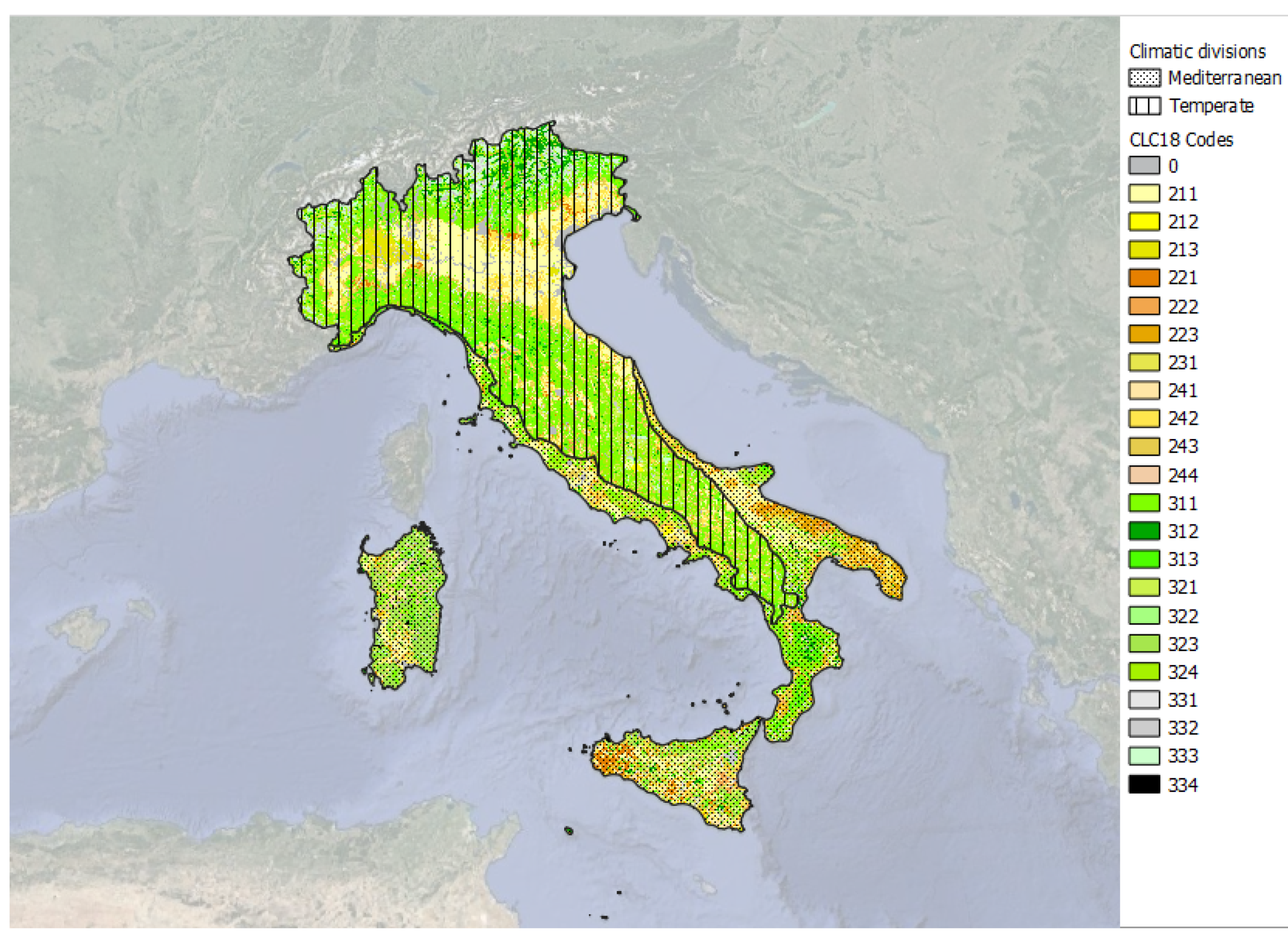
2. Study Area
3. Materials and Methods
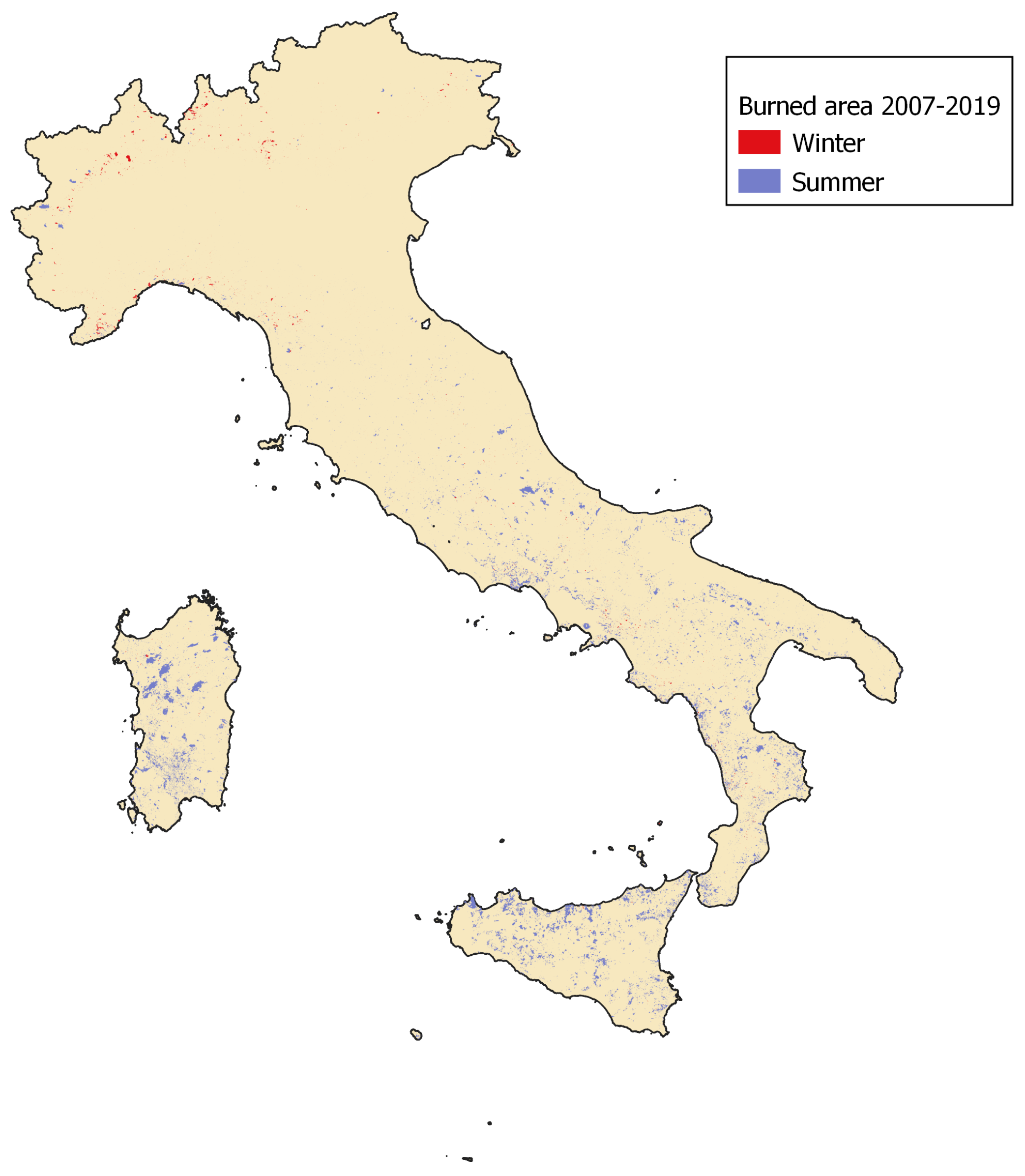
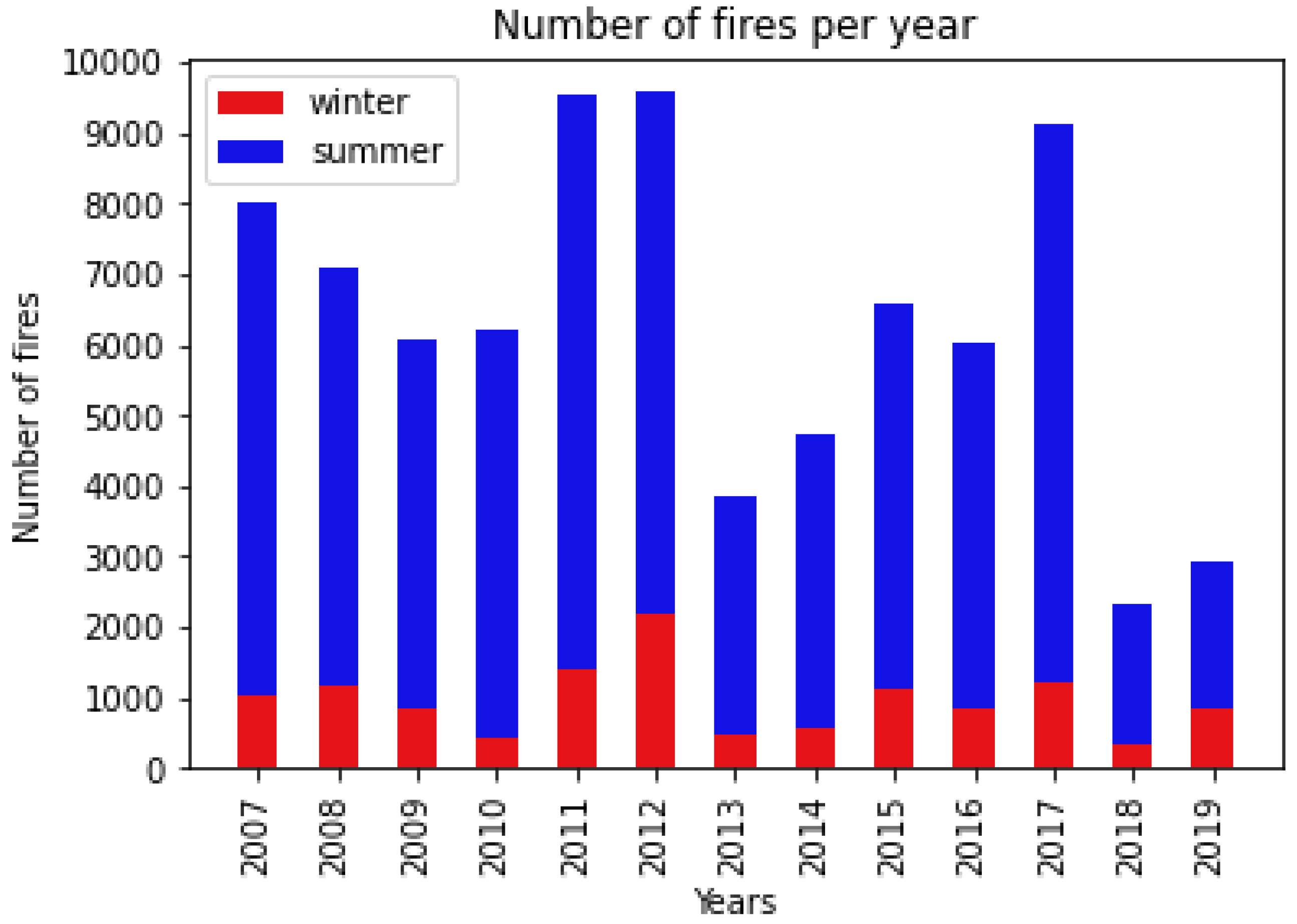
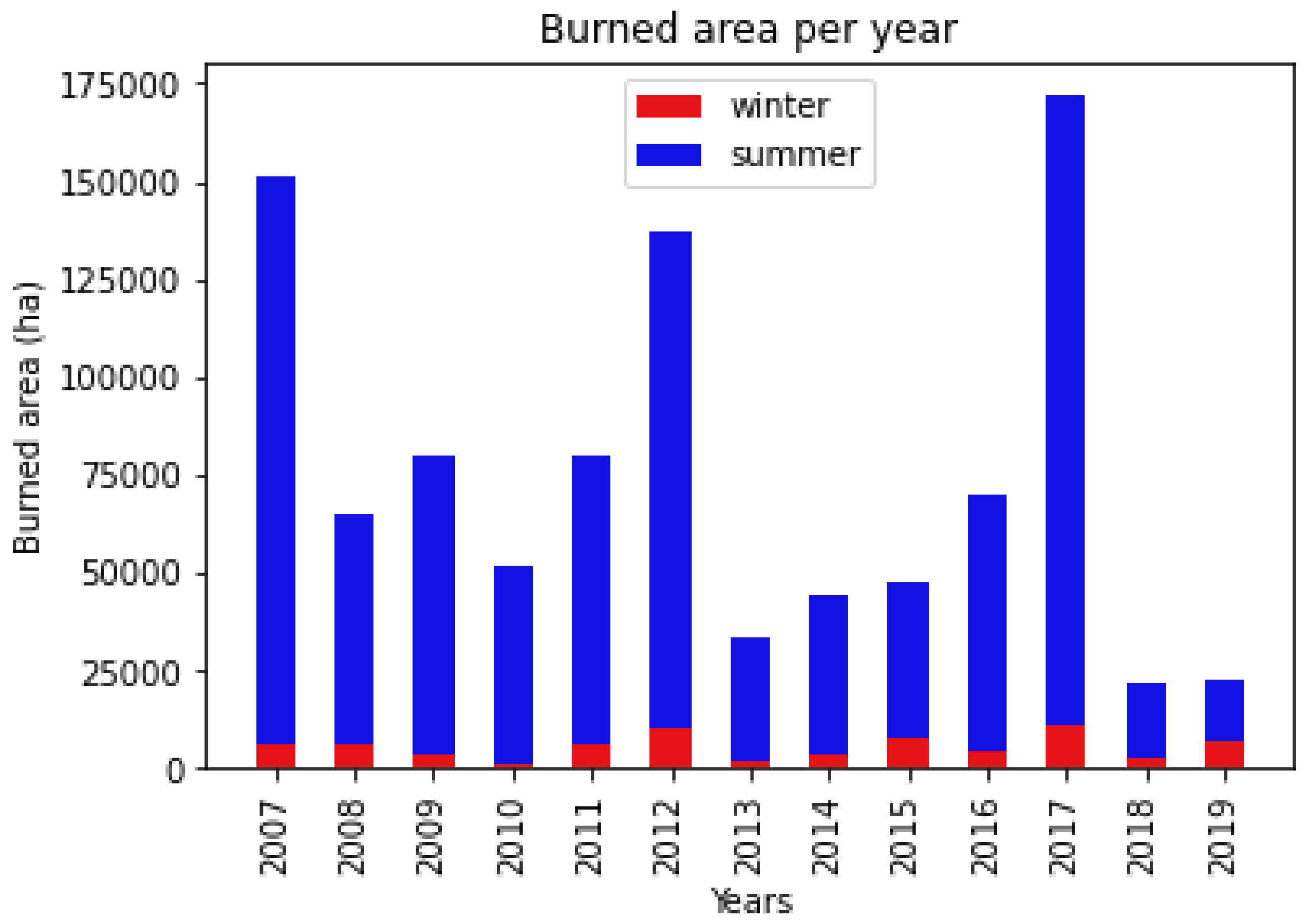
3.1. Historical Wildfire Database
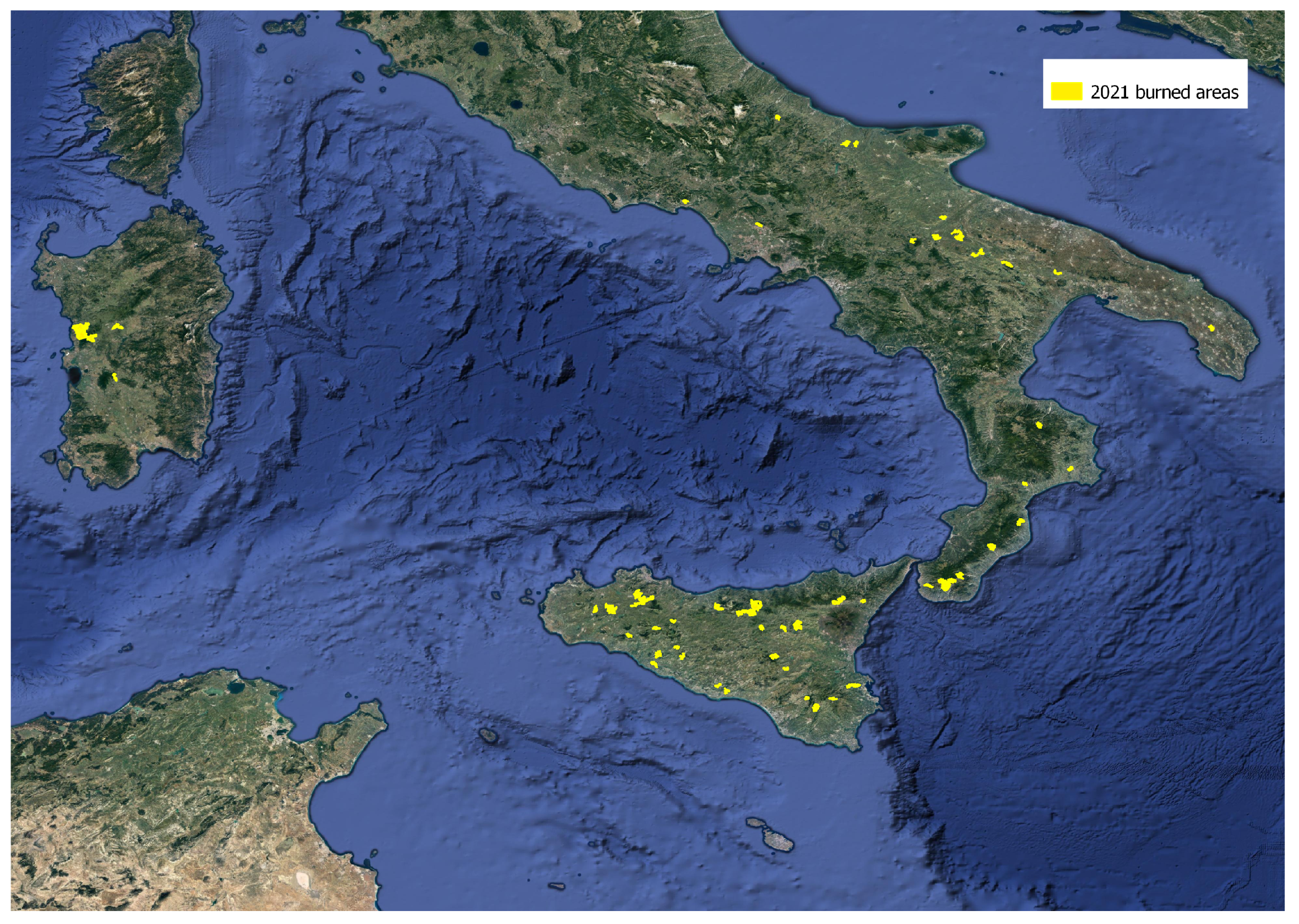
3.2. Additional Wildfire Data-Set for Model Validation
3.3. The Predisposing Factors: Geo-Climatic and Anthropic Data-Set
Topographic Variables
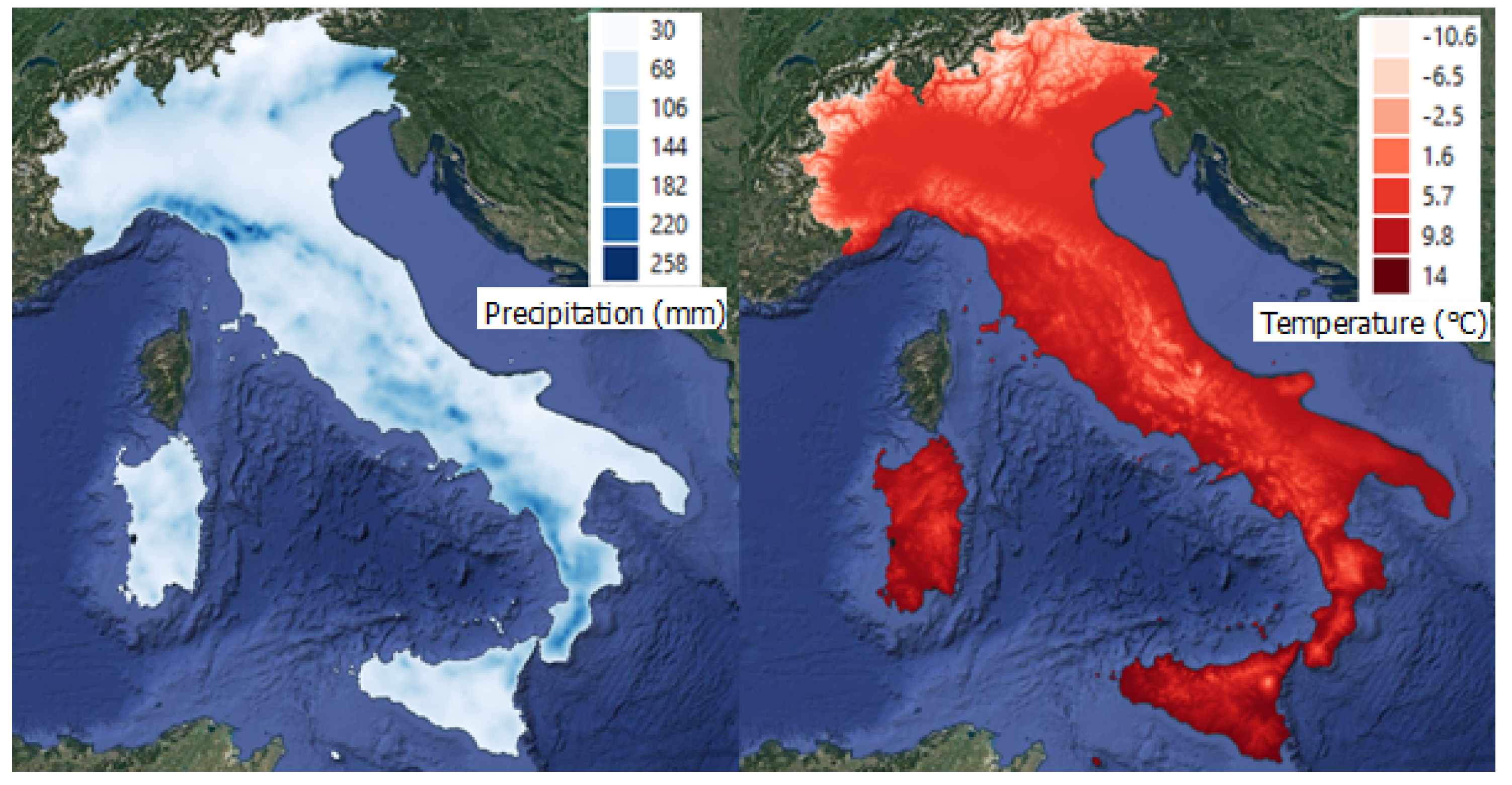
3.4. Climatic Variables
- Total Precipitation in winter and summer months, respectively; those layers represented the monthly cumulative precipitation (mm) from 1951 to 2019, averaged on the winter and summer wildfire season months, respectively.
- Mean Temperature in winter and summer months, respectively; those layers identify the mean average temperature (°C) from 1951 to 2019, averaged on the winter and summer wildfire season months, respectively.
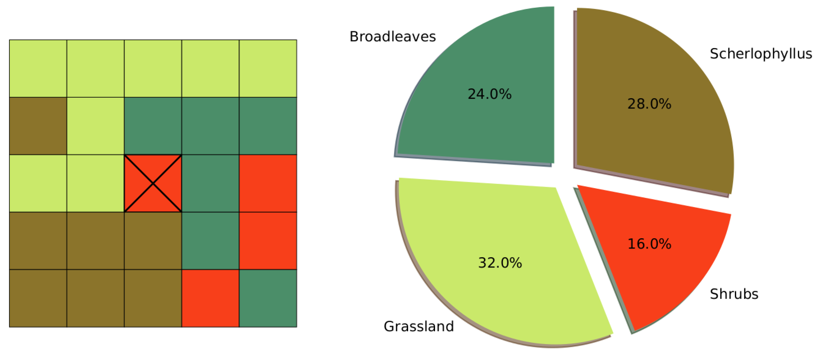
3.4.1. Vegetation Variables
3.4.2. Anthropic Variables
- the distance from the road network (m), obtained through processing of the SEDAC database [39];
- the distance from agricultural areas (m), obtained from the polygons of CLC18 land cover related to agricultural activities;
- the distance from settlements (m), obtained from CLC18 land cover polygons related to towns and settlements;
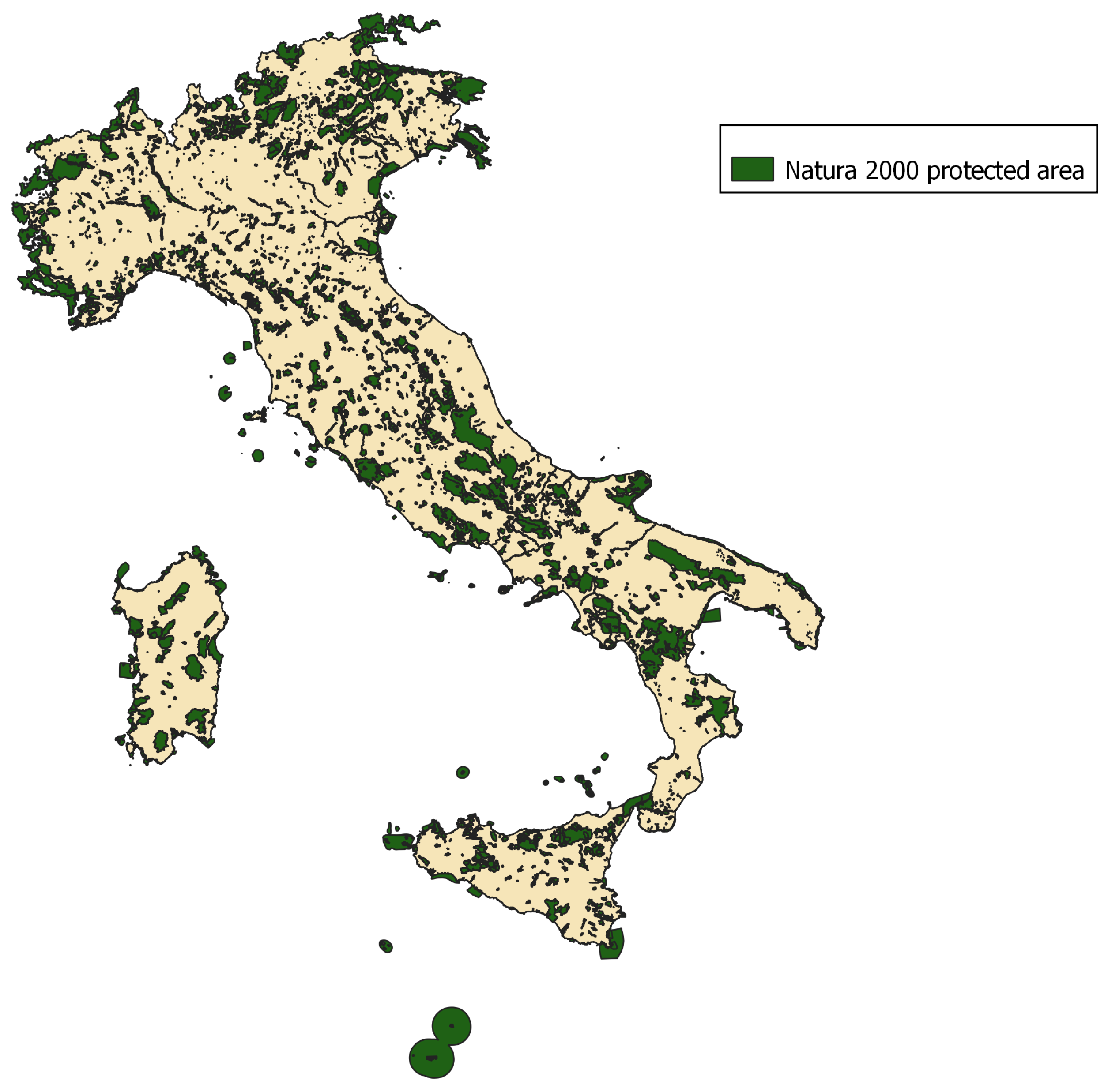
- the presence of Natura2000 protected areas (binary variable, 1 if the analyzed pixel falls into one of the areas reported by Natura2000 network, and 0 otherwise).
3.5. Methodology: The Machine Learning Model
3.5.1. Model Testing
- 1.
- The Mean Squared Error (MSE). This performance indicator is evaluated as follows:where n in the number of test pixels, represents the true label information (in a discrete fashion, with 1 standing for burned pixel and 0 for a non-burned one) and represents the label predicted by the continuous (probabilistic) output of the ML model.
- 2.
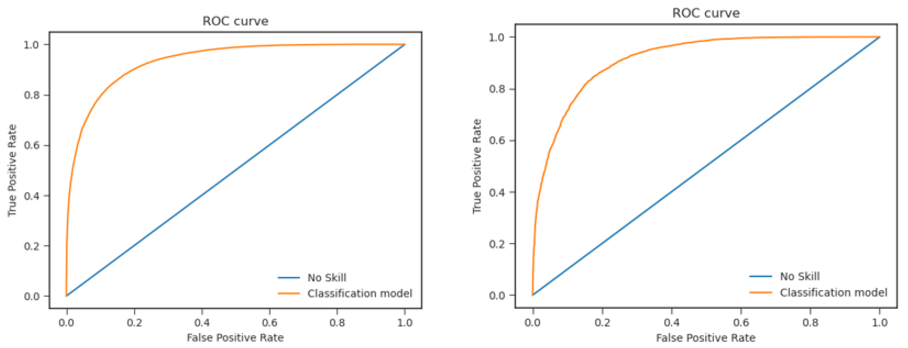
- ROC curves are computed using the prediction of the model on the test pixels. The related AUC is retrieved.
- 3.
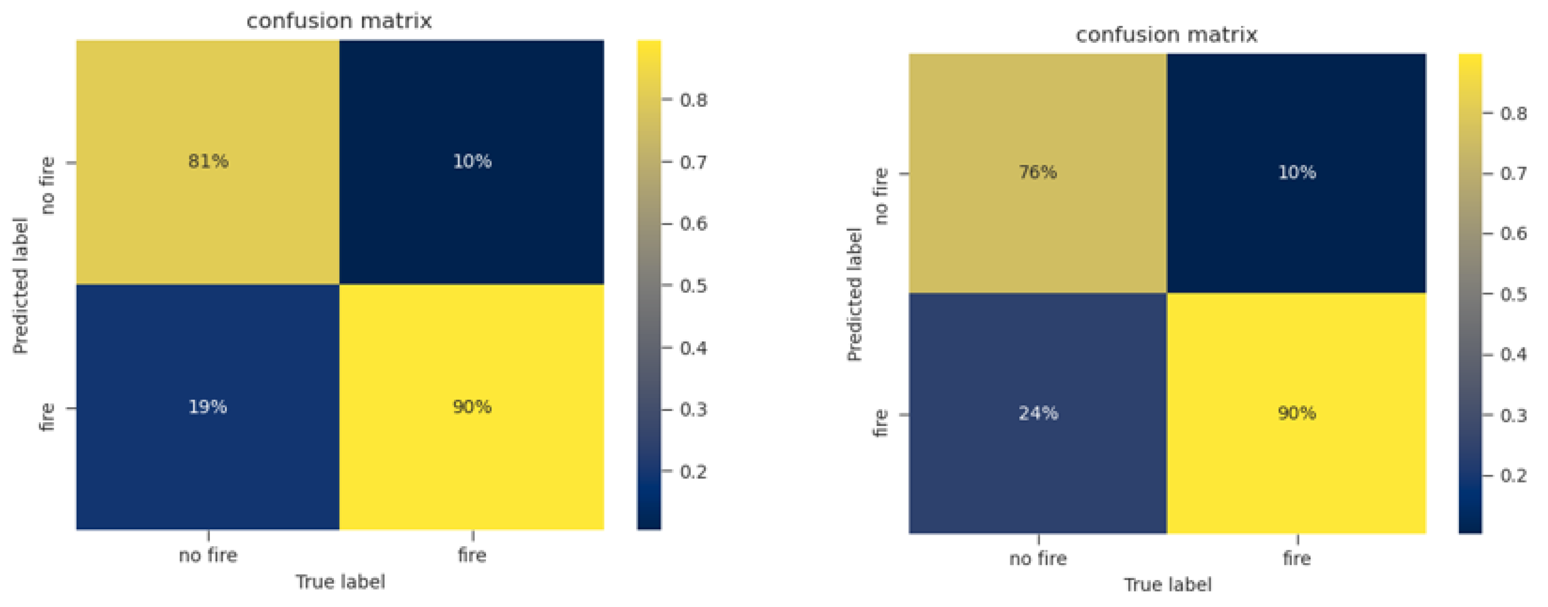
- The model accuracy over the testing data-set has been computed. It is here recalled that the overall accuracy of a binary classification model is defined aswhere , , , and stand for the four entries of the confusion matrix: True Positives, True Negatives, False Positives, False Negatives, respectively. The accuracy is the ratio between the correctly identified test data entries and the total size of the test set.
- 4.
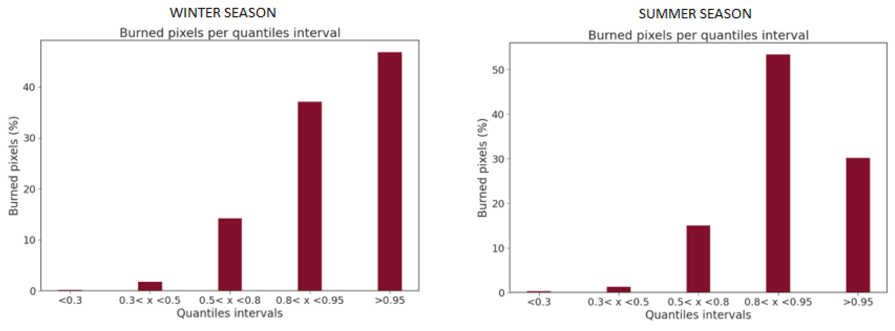
- The susceptibility map values have then been divided in groups, for both seasons, following predefined quantile ranges, which are shown in Table 2 [25]. The test pixels associated with past wildfires are then assigned to each of the classes and their distribution can be visualized in a histogram. If the susceptibility map is well built, most of the testing wildfire pixels should fall on the highest susceptibility classes.
3.5.2. Workflow
- 1.
- Gather the input layers for the predisposing factors, process them and align their spatial extent and projection; pre-process climate data season-wise.
- 2.
- Gather the shapefile data for wildfire occurrences, dividing it season-wise and rasterizing according to the working projection.
- 3.
- For each season, create an initial balanced database with random sampling for pseudo-absences (pixels not touched by wildfires).
- 4.
- Split the database into train and test sets.
- 5.
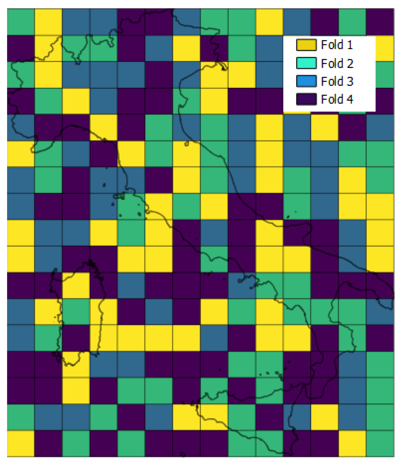
- For the training database, perform a 4-fold spatial cross validation building four different RF models and evaluating ROC AUC.
- 6.
- Build the RF model from the entire training set.
- 7.
- Compute performance indicators and variable importance ranking.
- 8.
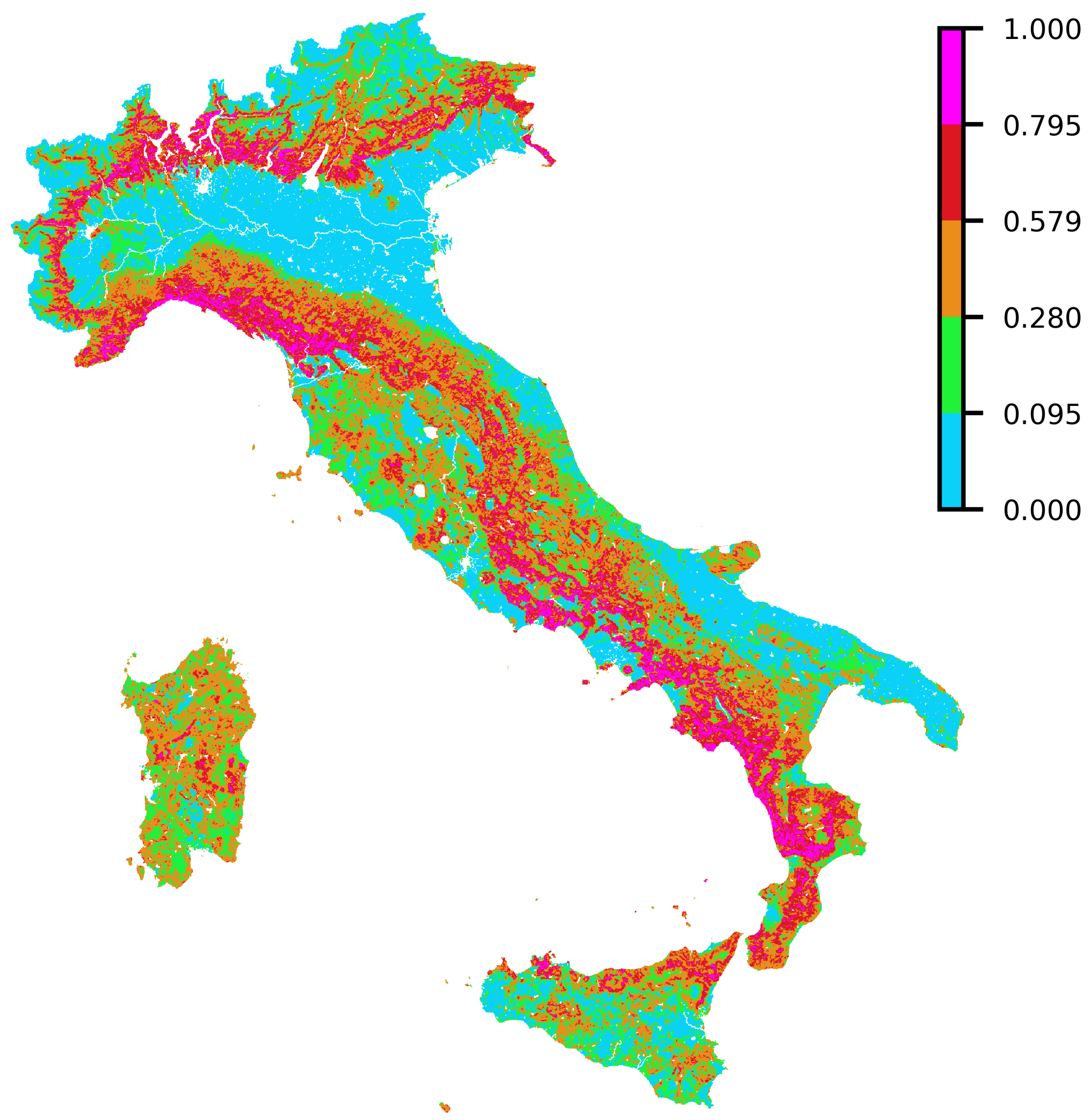
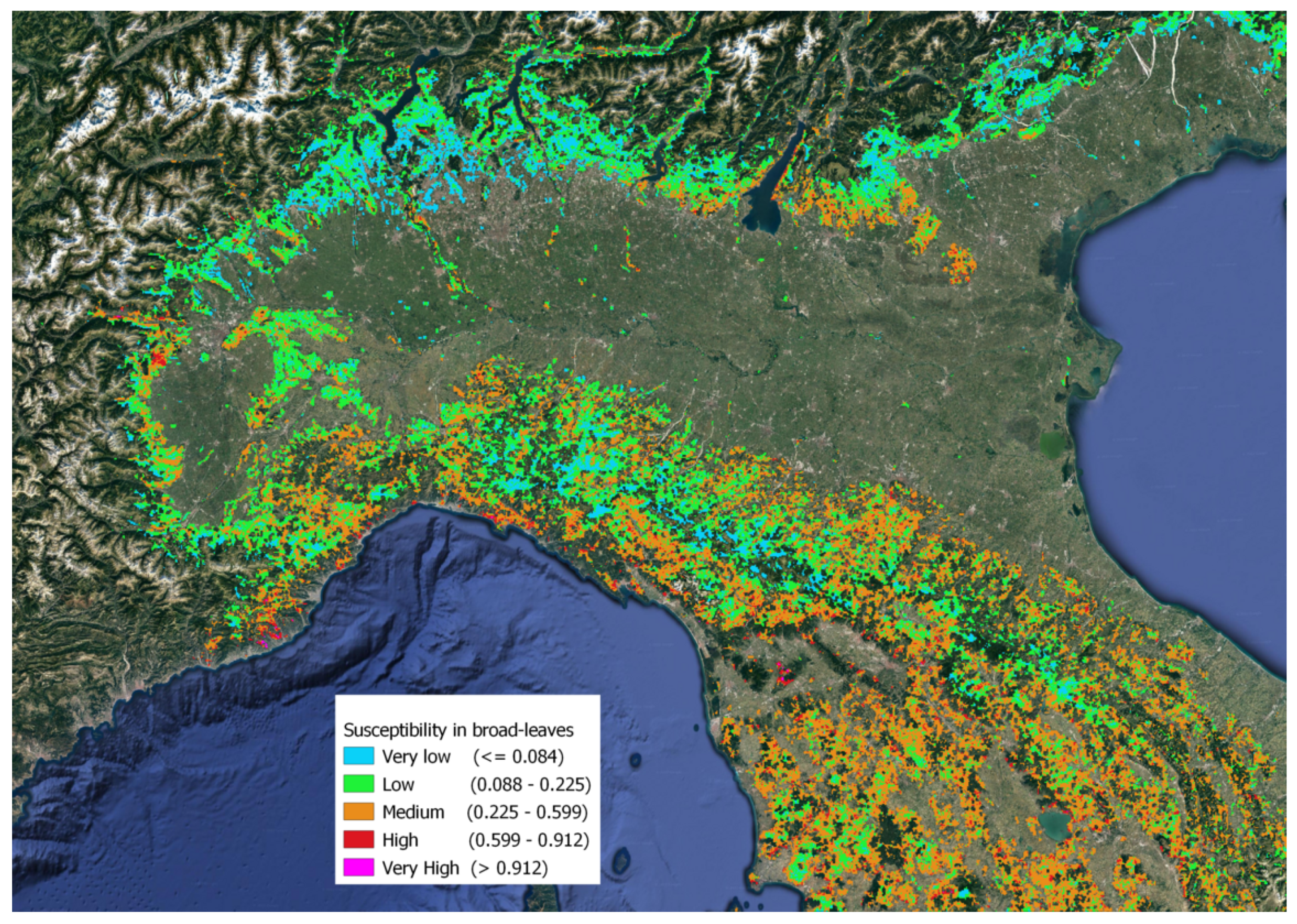
- Evaluate the model for every pixel of the entire Study Area, in order to obtain the Susceptibility Map.
- 9.
- Compute quantiles of the Susceptibility Map and check the susceptibility distribution of the test burned pixels.
4. Results
4.1. Spatial Cross Validation
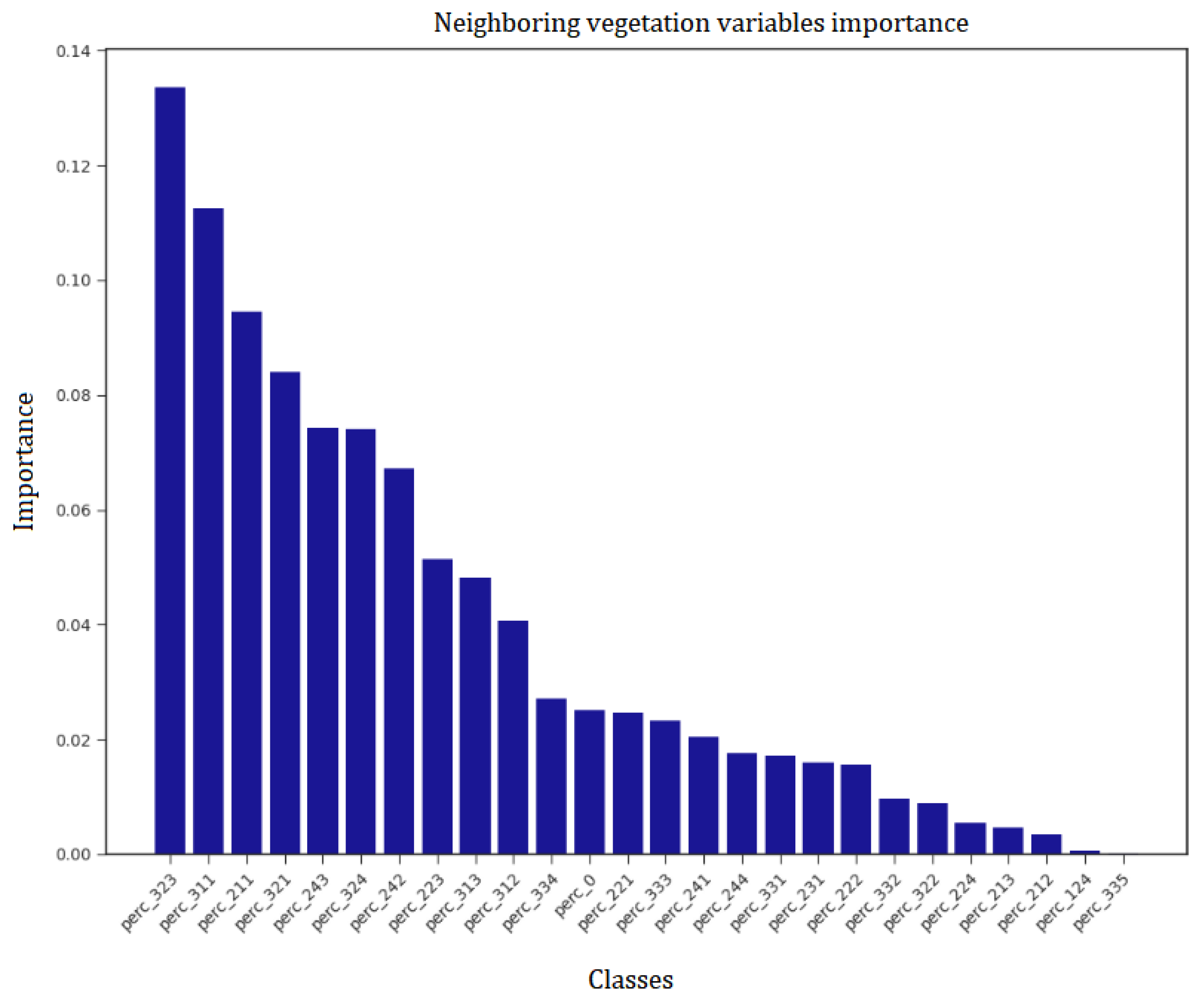
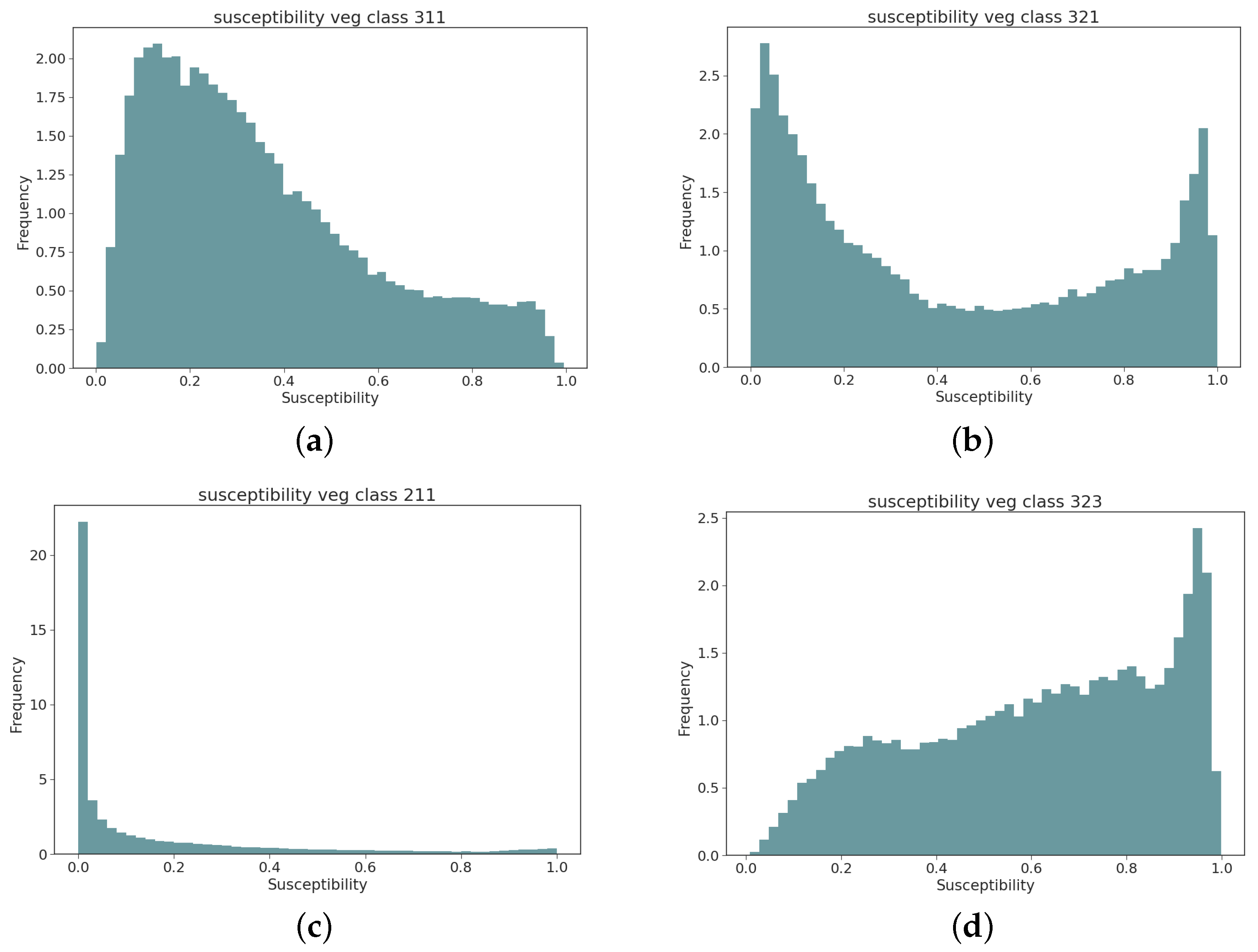
4.2. Input Features Ranking
4.3. Testing Phase: Performance Indicators
4.4. Quantiles Analysis: Distribution of Susceptibility over the Test Set Burned Pixels
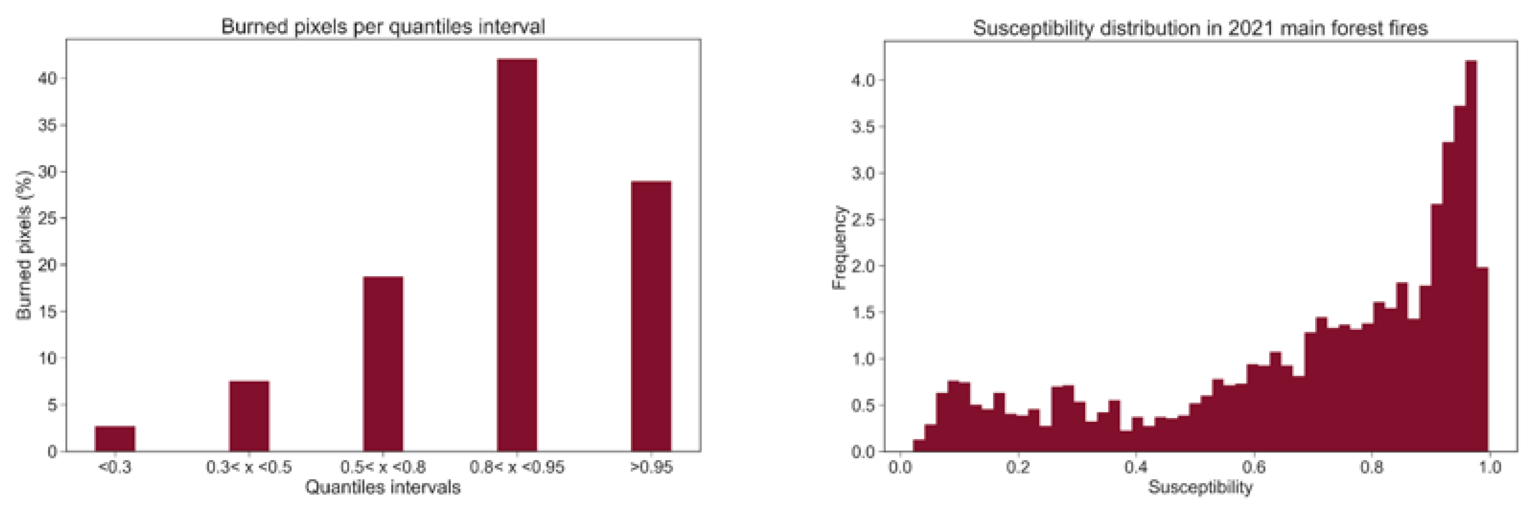
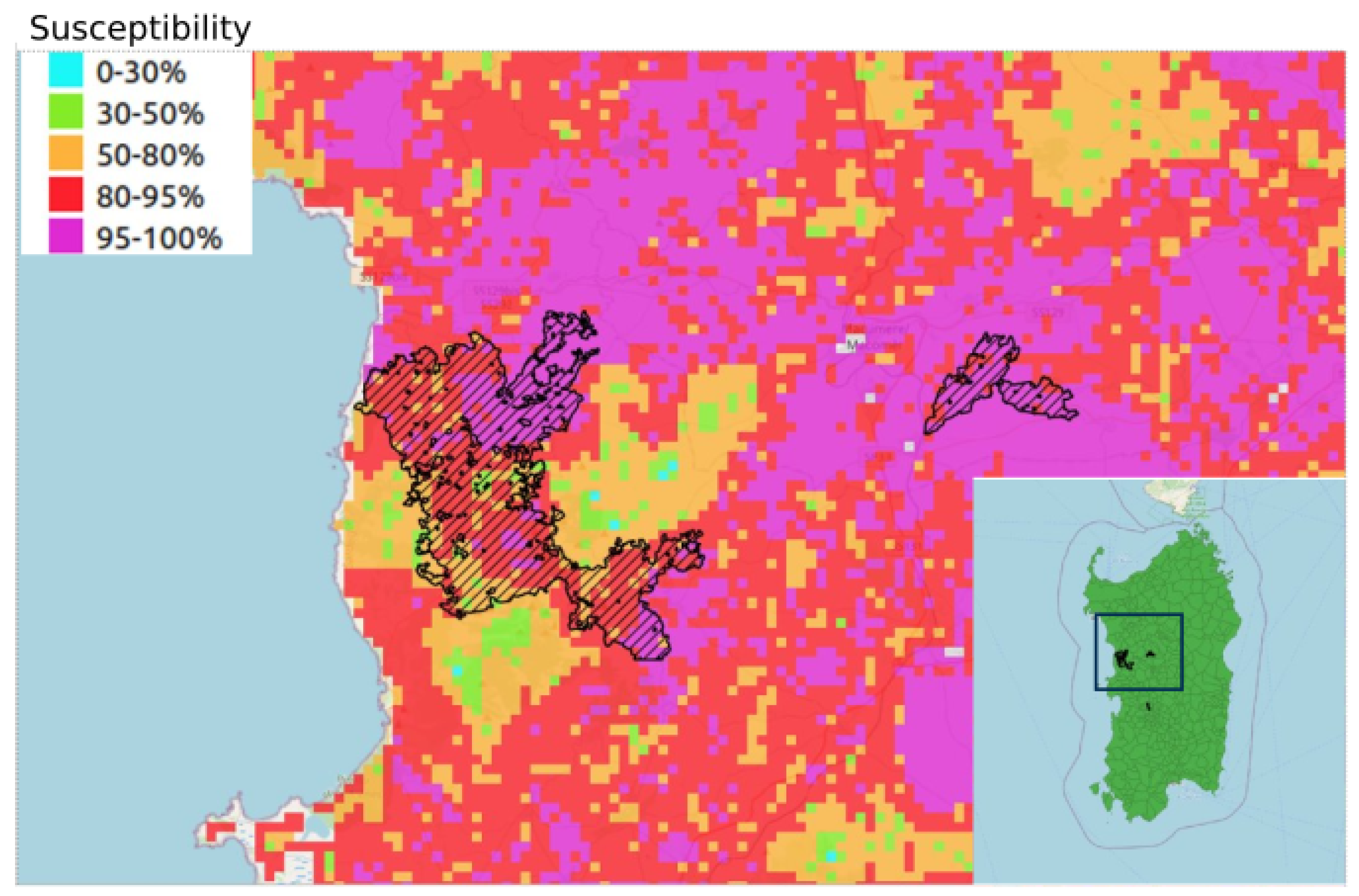
4.5. Quantile Analysis: Distribution of Susceptibility over a Set of Satellite-Retrieved Burned Areas from the 2021 Season
5. Discussion
6. Conclusions
Supplementary Materials
Author Contributions
Funding
Acknowledgments
Conflicts of Interest
Abbreviations
| CLC | CORINE Land Cover |
| ML | Machine Learning |
| DEM | Digital Elevation Model |
| AUC | Area under the ROC curve |
| CV | Cross Validation |
References
- San-Miguel-Ayanz, J.; Durrant, T.; Boca, R.; Maianti, P.; Libertà, G.; Artes Vivancos, T.; Jacome Felix Oom, D.; Branco, A.; De Rigo, D.; Ferrari, D.; et al. Advance EFFIS Report on Forest Fires in Europe, Middle East and North Africa 2020. Available online: https://publications.jrc.ec.europa.eu/repository/handle/JRC124833 (accessed on 20 December 2021).
- European Commission; Directorate-General for Environment; Sundseth, K. Natura 2000: Protecting Europe’s Biodiversity; European Commission: Luxembourg, 2008. [Google Scholar]
- Turco, M.; Bedia, J.; Liberto, F.; Fiorucci, P.; Hardenberg, J.; Koutsias, N.; Llasat, M.; Xystrakis, F.; Provenzale, A. Decreasing Fires in Mediterranean Europe. PLoS ONE 2016, 11, e0150663. [Google Scholar] [CrossRef] [Green Version]
- Faivre, N.; Xanthopoulos, F.; Moreno, J.; Calzada, V.; Xanthopoulos, G. Forest Fires–Sparking Firesmart Policies in the EU; Publications Office of the European Union: Luxembourg, 2018.
- San-Miguel-Ayanz, J.; Durrant, T.; Boca, R.; Maianti, P.; Libertà, G.; Artes Vivancos, T.; Jacome Felix Oom, D.; Branco, A.; De Rigo, D.; Ferrari, D.; et al. Advance EFFIS Report on Forest Fires in Europe, Middle East and North Africa 2019. 2020. Available online: https://publications.jrc.ec.europa.eu/repository/handle/JRC120692 (accessed on 20 December 2021).
- Bergonse, R.; Oliveira, S.; Gonçalves, A.; Nunes, S.; da Câmara, C.; Zêzere, J.L. A combined structural and seasonal approach to assess wildfire susceptibility and hazard in summertime. Nat. Hazards 2021, 106, 2545–2573. [Google Scholar] [CrossRef]
- Leuenberger, M.; Parente, J.; Tonini, M.; Pereira, M.G.; Kanevski, M. Wildfire susceptibility mapping: Deterministic vs. stochastic approaches. Environ. Model. Softw. 2018, 101, 194–203. [Google Scholar] [CrossRef]
- Cao, Y.; Wang Ming, L.K. Wildfire Susceptibility Assessment in Southern China: A Comparison of Multiple Methods. Int. J. Disaster Risk Sci. 2017, 8, 164–181. [Google Scholar] [CrossRef] [Green Version]
- Zhang, G.; Wang, M.; Liu, K. Deep neural networks for global wildfire susceptibility modelling. Ecol. Indic. 2021, 127, 107735. [Google Scholar] [CrossRef]
- Juliao, R.; Nery, F.; Ribeiro, J.; Branco, M.; Zêzere, J. Guia Metodológico Para a Produção de Cartografia Municipal de Risco e Para a Criação de Sistemas de Informação Geográfica de Base Municipal. 2009. Available online: https://repositorio.ul.pt/handle/10451/39562 (accessed on 20 December 2021).
- Jaafari, A.; Mafi-Gholami, D.; Thai Pham, B.; Tien Bui, D. Wildfire Probability Mapping: Bivariate vs. Multivariate Statistics. Remote Sens. 2019, 11, 618. [Google Scholar] [CrossRef] [Green Version]
- Hong, H.; Sun, Z. Applying SDN for Data Extraction and Mining: An Enhanced Architecture. Natl. Acad. Sci. Lett. 2017, 40, 167–169. [Google Scholar] [CrossRef]
- Chhetri, S.K.; Kayastha, P. Manifestation of an Analytic Hierarchy Process (AHP) Model on Fire Potential Zonation Mapping in Kathmandu Metropolitan City, Nepal. ISPRS Int. J. -Geo-Inf. 2015, 4, 400–417. [Google Scholar] [CrossRef] [Green Version]
- Gregorio, S.D.; Filippone, G.; Spataro, W.; Trunfio, G. Accelerating wildfire susceptibility mapping through GPGPU. J. Parallel Distrib. Comput. 2013, 73, 1183–1194. [Google Scholar] [CrossRef]
- Parisien, M.A.; Kafka, V.; Hirsch, K.; Todd, J.; Lavoie, S.G.; Maczek, P. Mapping Wildfire Susceptibility with the BURN-P3 Simulation Model; Technical Report Information Report NOR-X-405; Natural Resources Canada, Canadian Forest Service, Northern Forestry Centre: Edmonton, AB, Canada, 2005.
- Darabi, H.; Choubin, B.; Rahmati, O.; Torabi Haghighi, A.; Pradhan, B.; Kløve, B. Urban flood risk mapping using the GARP and QUEST models: A comparative study of machine learning techniques. J. Hydrol. 2019, 569, 142–154. [Google Scholar] [CrossRef]
- Hong, H.; Shahabi, H.; Shirzadi, A.; Chen, W.; Chapi, K.; Ahmad, B.B.; Roodposhti, M.S.; Yari Hesar, A.; Tian, Y.; Tien Bui, D. Landslide susceptibility assessment at the Wuning area, China: A comparison between multi-criteria decision-making, bivariate statistical and machine learning methods. Nat. Hazards 2019, 96, 173–212. [Google Scholar] [CrossRef]
- Nhu, V.H.; Zandi, D.; Shahabi, H.; Chapi, K.; Shirzadi, A.; Al-Ansari, N.; Singh, S.K.; Dou, J.; Nguyen, H. Comparison of Support Vector Machine, Bayesian Logistic Regression, and Alternating Decision Tree Algorithms for Shallow Landslide Susceptibility Mapping along a Mountainous Road in the West of Iran. Appl. Sci. 2020, 10, 5047. [Google Scholar] [CrossRef]
- Ghorbanzadeh, O.; valizadeh kamran, K.; Blaschke, T.; Aryal, J.; Naboureh, A.; Einali, J.; Bian, J. Spatial Prediction of Wildfire Susceptibility Using Field Survey GPS Data and Machine Learning Approaches. Fire 2019, 2, 43. [Google Scholar] [CrossRef] [Green Version]
- Ghorbanzadeh, O.; Blaschke, T.; Gholamnia, K.; Aryal, J. Forest Fire Susceptibility and Risk Mapping Using Social/Infrastructural Vulnerability and Environmental Variables. Fire 2019, 2, 50. [Google Scholar] [CrossRef] [Green Version]
- Rodrigues, M.; de la Riva, J. An insight into machine-learning algorithms to model human-caused wildfire occurrence. Environ. Model. Softw. 2014, 57, 192–201. [Google Scholar] [CrossRef]
- Thach, N.N.; Ngo, D.B.T.; Xuan-Canh, P.; Hong-Thi, N.; Thi, B.H.; Nhat-Duc, H.; Dieu, T.B. Spatial pattern assessment of tropical forest fire danger at Thuan Chau area (Vietnam) using GIS-based advanced machine learning algorithms: A comparative study. Ecol. Inform. 2018, 46, 74–85. [Google Scholar] [CrossRef]
- Safi, Y.; Bouroumi, A. Prediction of forest fires using Artificial neural networks. Appl. Math. Sci. 2013, 7, 271–286. [Google Scholar] [CrossRef]
- Ma, W.; Feng, Z.; Cheng, Z.; Chen, S.; Wang, F. Identifying Forest Fire Driving Factors and Related Impacts in China Using Random Forest Algorithm. Forests 2020, 11, 507. [Google Scholar] [CrossRef]
- Tonini, M.; D’Andrea, M.; Biondi, G.; Degli Esposti, S.; Trucchia, A.; Fiorucci, P. A Machine Learning-Based Approach for Wildfire Susceptibility Mapping. The Case Study of the Liguria Region in Italy. Geosciences 2020, 10, 105. [Google Scholar] [CrossRef] [Green Version]
- Yang, H.; Li, S.; Chen, J.; Zhang, X.; Xu, S. The Standardization and Harmonization of Land Cover Classification Systems towards Harmonized Datasets: A Review. ISPRS Int. J.-Geo-Inf. 2017, 6, 154. [Google Scholar] [CrossRef] [Green Version]
- Michetti, M.; Pinar, M. Forest fires across Italian regions and implications for climate change: A panel data analysis. Environ. Resour. Econ. 2019, 72, 207–246. [Google Scholar] [CrossRef] [Green Version]
- Ganteaume, A.; Barbero, R.; Jappiot, M.; Maillé, E. Understanding future changes to fires in southern Europe and their impacts on the wildland-urban interface. J. Saf. Sci. Resil. 2021, 2, 20–29. [Google Scholar] [CrossRef]
- Blasi, C.; Boitani, L.; La Posta, S.; Manes, F.; Marchetti, M. Biodiversity in Italy. Contribution to the National Strategy of Biodiversity. 2007. Available online: https://www.semanticscholar.org/paper/BIODIVERSITY-IN-ITALY.-CONTRIBUTION-TO-THE-NATIONAL-Blasi-Boitani/6e3d721f87a8e99b04547c7bdd274a9232563f81 (accessed on 20 December 2021).
- Blasi, C.; Capotorti, G.; Copiz, R.; Guida, D.; Mollo, B.; Smiraglia, D.; Zavattero, L. Map of the Terrestrial Ecoregions of Italy, 1: 1 000 000. 2019. Available online: https://www.researchgate.net/publication/337276053_Map_of_the_Terrestrial_Ecoregions_of_Italy_1_1_000_000 (accessed on 20 December 2021).
- Blasi, C.; Capotorti, G.; Copiz, R.; Guida, D.; Mollo, B.; Smiraglia, D.; Zavattero, L.; Zavattero, L. Terrestrial Ecoregions of Italy Explanatory Notes. 2019. Available online: https://www.researchgate.net/publication/337275982_Terrestrial_Ecoregions_of_Italy_explanatory_notes (accessed on 20 December 2021).
- European Environment Agency; Feranec, J.; Büttner, G.; Jaffrain, G. Corine Land Cover Update 2000; European Environment Agency. 2003. Available online: https://land.copernicus.eu/pan-european/corine-land-cover/clc-2000 (accessed on 20 December 2021).
- Pulvirenti, L.; Squicciarino, G.; Fiori, E.; Fiorucci, P.; Ferraris, L.; Negro, D.; Gollini, A.; Severino, M.; Puca, S. An Automatic Processing Chain for Near Real-Time Mapping of Burned Forest Areas Using Sentinel-2 Data. Remote Sens. 2020, 12, 674. [Google Scholar] [CrossRef] [Green Version]
- Pulvirenti, L.; Squicciarino, G.; Fiori, E. A Method to Automatically Detect Changes in Multitemporal Spectral Indices: Application to Natural Disaster Damage Assessment. Remote Sens. 2020, 12, 2681. [Google Scholar] [CrossRef]
- Olaya, V. Basic Land-Surface Parameters. In Geomorphometry. Concepts, Software, Applications. Developments in Soil Science, Volume 33; Hengl, T., Reuter, H., Eds.; Elsevier: Amsterdam, The Netherlands, 2009. [Google Scholar]
- Braca, G.; Ducci, D. Development of a GIS Based Procedure (BIGBANG 1.0) for Evaluating Groundwater Balances at National Scale and Comparison with Groundwater Resources Evaluation at Local Scale. In Groundwater and Global Change in the Western Mediterranean Area; Calvache, M.L., Duque, C., Pulido-Velazquez, D., Eds.; Springer International Publishing: Cham, Switzerland, 2018; pp. 53–61. [Google Scholar]
- Braca, G.; Bussettini, M.; Lastoria, B.; Mariani, S.; Piva, F. Elaborazioni Modello BIGBANG Versione 4.0; Technical Report; Istituto Superiore per la Protezione e la Ricerca Ambientale— ISPRA: Roma, Italy, 2021.
- Corine Land Cover (CLC) 2018, Version 2020_20u1. Available online: https://land.copernicus.eu/pan-european/corine-land-cover/clc2018? (accessed on 30 December 2021).
- Global Roads Open Access Data Set, Version 1 (gROADSv1); Technical Report; Center for International Earth Science Information Network—CIESIN—Columbia University and Information Technology Outreach Services—ITOS—University of Georgia, NASA Socioeconomic Data and Applications Center (SEDAC): Palisades, NY, USA, 2013.
- Breiman, L. Random Forests. Mach. Learn. 2001, 45, 5–32. [Google Scholar] [CrossRef] [Green Version]
- Pedregosa, F.; Varoquaux, G.; Gramfort, A.; Michel, V.; Thirion, B.; Grisel, O.; Blondel, M.; Prettenhofer, P.; Weiss, R.; Dubourg, V.; et al. Scikit-learn: Machine Learning in Python. J. Mach. Learn. Res. 2011, 12, 2825–2830. [Google Scholar]
- Probst, P.; Wright, M.N.; Boulesteix, A.L. Hyperparameters and tuning strategies for random forest. WIREs Data Min. Knowl. Discov. 2019, 9, e1301. [Google Scholar] [CrossRef] [Green Version]
- Kotsiantis, S.; Kanellopoulos, D.; Pintelas, P. Handling imbalanced datasets: A review. GESTS Int. Trans. Comput. Sci. Eng. 2005, 30, 25–36. [Google Scholar]
- Moayedi, H.; Mehrabi, M.; Bui, D.T.; Pradhan, B.; Foong, L.K. Fuzzy-metaheuristic ensembles for spatial assessment of forest fire susceptibility. J. Environ. Manag. 2020, 260, 109867. [Google Scholar] [CrossRef] [PubMed]
- Vilar, L.; Gómez, I.; Martínez-Vega, J.; Echavarría, P.; Riaño, D.; Martín, M.P. Multitemporal Modelling of Socio-Economic Wildfire Drivers in Central Spain between the 1980s and the 2000s: Comparing Generalized Linear Models to Machine Learning Algorithms. PLoS ONE 2016, 11, e0161344. [Google Scholar] [CrossRef] [PubMed] [Green Version]
- Ishwaran, H. The effect of splitting on random forests. Mach. Learn. 2015, 99, 75–118. [Google Scholar] [CrossRef]
- Breiman, L. Manual on Setting Up, Using, and Understanding Random Forests v3.1; Statistics Department University of California Berkeley: Berkeley, CA, USA, 2002; Volume 1. [Google Scholar]
- Louppe, G. Understanding Random Forests: From Theory to Practice. Ph.D. Thesis. 2014. Available online: https://doi.org/10.13140/2.1.1570.5928 (accessed on 20 December 2021).
- Hancock, J.T.; Khoshgoftaar, T.M. Survey on categorical data for neural networks. J. Big Data 2020, 7, 28. [Google Scholar] [CrossRef] [Green Version]
- Novo, A.; Fariñas-Álvarez, N.; Martínez-Sánchez, J.; González-Jorge, H.; Fernández-Alonso, J.M.; Lorenzo, H. Mapping Forest Fire Risk—A Case Study in Galicia (Spain). Remote Sens. 2020, 12, 3705. [Google Scholar] [CrossRef]
- Oliveira, S.; Gonçalves, A.; Zêzere, J.L. Reassessing wildfire susceptibility and hazard for mainland Portugal. Sci. Total Environ. 2021, 762, 143121. [Google Scholar] [CrossRef]
- Marchese, F.; Mazzeo, G.; Filizzola, C.; Coviello, I.; Falconieri, A.; Lacava, T.; Paciello, R.; Pergola, N.; Tramutoli, V. Issues and Possible Improvements in Winter Fires Detection by Satellite Radiances Analysis: Lesson Learned in Two Regions of Northern Italy. IEEE J. Sel. Top. Appl. Earth Obs. Remote Sens. 2017, 10, 3297–3313. [Google Scholar] [CrossRef]
- Vacchiano, G.; Foderi, C.; Berretti, R.; Marchi, E.; Motta, R. Modeling anthropogenic and natural fire ignitions in an inner-alpine valley. Nat. Hazards Earth Syst. Sci. 2018, 18, 935–948. [Google Scholar] [CrossRef] [Green Version]
- Sullivan, A.L. Wildland surface fire spread modelling, 1990–2007. 1: Physical and quasi-physical models. Int. J. Wildland Fire 2009, 18, 349–368. [Google Scholar] [CrossRef] [Green Version]
- Sullivan, A. Wildland surface fire spread modelling, 1990–2007. 2: Empirical and quasi-empirical models. Int. J. Wildland Fire 2009, 18, 369–386. [Google Scholar] [CrossRef] [Green Version]
- Sullivan, A. Wildland surface fire spread modelling, 1990–2007. 3: Simulation and mathematical analogue models. Int. J. Wildland Fire 2009, 18, 387–403. [Google Scholar] [CrossRef] [Green Version]
- Trucchia, A.; D’Andrea, M.; Baghino, F.; Fiorucci, P.; Ferraris, L.; Negro, D.; Gollini, A.; Severino, M. PROPAGATOR: An Operational Cellular-Automata Based Wildfire Simulator. Fire 2020, 3, 26. [Google Scholar] [CrossRef]
- Fiorucci, P.; Gaetani, F.; Minciardi, R. Development and application of a system for dynamic wildfire risk assessment in Italy. Environ. Model. Softw. 2008, 23, 690–702. [Google Scholar] [CrossRef]
- Fiorucci, P.; D’Andrea, M.; Negro, D.; Severino, M. Manuale d’uso del Sistema Previsionale Della Pericolosità Potenziale Degli Incendi Boschivi RIS.I.CO; Technical Report; Italian Department of Civil Protection—Presidency of the Council of Ministers, and CIMA Research Foundation: Roma, Italy, 2011.
- Fiorucci, P.; D’Andrea, M.; Negro, D.; Gollini, A.; Severino, M. I Aggiornamento del Manuale d’uso del Sistema Previsionale della Pericolosità Potenziale Degli Incendi Boschivi RIS.I.CO. –RISICO; Technical Report; Italian Department of Civil Protection—Presidency of the Council of Ministers, and CIMA Research Foundation: Roma, Italy, 2015.


| Variable Name | Variable Type | No. of Variables |
|---|---|---|
| DEM | Numerical (meters) | 1 |
| Slope | Numerical (degree) | 1 |
| Northness and Eastness | Numerical | 2 |
| Distance to anthropogenic features | Numerical (meters) | 4 |
| Area Natura 2000 | Binary | 1 |
| Vegetation type | Categorical (24 classes) | 1 |
| Mean Temperature, Mean Precipitation | Numerical(°C and mm) | 2 |
| Neighboring vegetation | Numerical (percentage) | 24 |
| Susceptibility Class | Quantiles Range |
|---|---|
| Very Low | 0–0.30 |
| Low | 0.30–0.50 |
| Medium | 0.50–0.80 |
| High | 0.80–0.95 |
| Very High | 0.95–1 |
| Season | AUC Fold 1–4 |
|---|---|
| Winter | [0.85 - 0.80 - 0.84 - 0.83] |
| Summer | [0.84 - 0.80 - 0.82 - 0.87] |
| Winter | Importance | Summer | Importance |
|---|---|---|---|
| Neighbour. Veg. | 0.30 | Neighbour. Veg. | 0.29 |
| Precipitation | 0.12 | Precipitation | 0.15 |
| Slope | 0.09 | Temperature | 0.11 |
| DEM | 0.08 | Slope | 0.08 |
| Temperature | 0.07 | DEM | 0.07 |
| Vegetation | 0.06 | Vegetation | 0.05 |
| North | 0.06 | Urban Dist. | 0.05 |
| Urban Dist | 0.05 | North | 0.05 |
| East | 0.04 | East | 0.04 |
| Roads Dist. | 0.04 | Roads Dist. | 0.04 |
| Crops Dist. | 0.02 | Crops Dist. | 0.02 |
| Natura 2000 | 0.01 | Natura 2000 | 0.01 |
| Season | ROC AUC | MSE | Overall Accuracy |
|---|---|---|---|
| Summer | 0.93 | 0.107 | 0.85 |
| Winter | 0.91 | 0.122 | 0.83 |
Publisher’s Note: MDPI stays neutral with regard to jurisdictional claims in published maps and institutional affiliations. |
© 2022 by the authors. Licensee MDPI, Basel, Switzerland. This article is an open access article distributed under the terms and conditions of the Creative Commons Attribution (CC BY) license (https://creativecommons.org/licenses/by/4.0/).
Share and Cite
Trucchia, A.; Meschi, G.; Fiorucci, P.; Gollini, A.; Negro, D. Defining Wildfire Susceptibility Maps in Italy for Understanding Seasonal Wildfire Regimes at the National Level. Fire 2022, 5, 30. https://doi.org/10.3390/fire5010030
Trucchia A, Meschi G, Fiorucci P, Gollini A, Negro D. Defining Wildfire Susceptibility Maps in Italy for Understanding Seasonal Wildfire Regimes at the National Level. Fire. 2022; 5(1):30. https://doi.org/10.3390/fire5010030
Chicago/Turabian StyleTrucchia, Andrea, Giorgio Meschi, Paolo Fiorucci, Andrea Gollini, and Dario Negro. 2022. "Defining Wildfire Susceptibility Maps in Italy for Understanding Seasonal Wildfire Regimes at the National Level" Fire 5, no. 1: 30. https://doi.org/10.3390/fire5010030
APA StyleTrucchia, A., Meschi, G., Fiorucci, P., Gollini, A., & Negro, D. (2022). Defining Wildfire Susceptibility Maps in Italy for Understanding Seasonal Wildfire Regimes at the National Level. Fire, 5(1), 30. https://doi.org/10.3390/fire5010030