Transition from the Space-Charge-Limited Regime to the Inverse Sheath Regime in a Thermionic Emissive Probe

Abstract

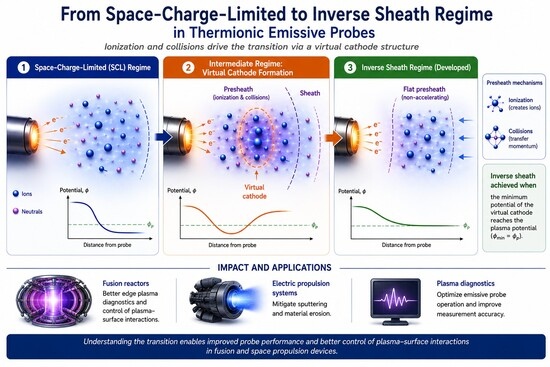
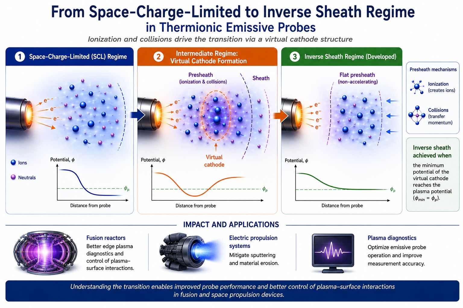
This article analyses the transition from the space-charge-limited (SCL) regime to the inverse sheath regime of a thermionic emissive probe, considering ionisation and collisions as presheath mechanisms. We show that, before the fully developed inverse sheath mode is reached, an intermediate regime appears, characterised by the formation of a virtual cathode structure with ion confinement and probe potentials above the plasma potential. The inverse sheath mode is reached when the minimum potential of the virtual cathode reaches the plasma potential. At this point, a monotonic sheath potential profile above the plasma potential is produced, together with a flat, non-accelerating presheath. The findings of this work can help optimise the performance of emissive probes in plasma diagnostics and control plasma–surface interactions in devices such as fusion reactors and electric propulsion systems, thereby mitigating sputtering and material erosion.

1. Introduction

The study of emissive surfaces began in the 1920s with the early work of Tonks and Langmuir [1,2,3], which was later continued by Hobbs and Wesson [4]. This kind of plasma–wall interaction features many processes and applications [5], such as sheaths and emissive probes [6,7,8], radiofrequency (RF) plasmas [9,10], Hall thrusters [11,12,13], magnetised plasmas [14,15], electron beams [16,17], and fusion plasmas [18,19,20,21,22,23]. In recent years, there has been special interest in the analysis of these types of interactions for highly emissive surfaces, either by secondary electron emission (SEE) [24,25,26,27,28,29,30,31,32,33,34] or thermoemission, including negative-ion emission [23,35,36,37,38,39,40].

At low emissions, when the probe or surface potential is lower than the plasma potential, the electric potential profile is monotonic. In this case, the probe or surface is said to operate in the temperature-limited (TL) regime or T-region of the I–V characteristic curve [41]. For higher emissions, a critical state, called the space-charge-limited (SCL) transition, is reached when the electric field becomes zero at the emitting surface [42]. A further increase in emission above this critical state causes the emitting surface to operate in the so-called SCL regime [11,14,43,44,45,46]. This regime is characterised by a double-sheath structure with a non-monotonic electric potential profile corresponding to a potential well, also known as a virtual cathode (VC), caused by the accumulation of negative charge in front of the surface [47,48,49]. As the emission coefficient or surface temperature increases, this cloud of negative charge limits and eventually saturates the net current emitted by the surface [42].

For a current-free emitting surface operating in this regime, the floating potential reaches a saturation value close to the plasma potential [11,13,14,42,43,44,45,50,51] and can therefore be used as an estimate of this plasma parameter. Some authors consider this saturation value to be of the order of $k_B{T}_e/e$ below the plasma potential [4,20,43]. However, several publications have questioned the stability of the SCL sheath, arguing that it is not compatible with the existence of ionisation and collisions [26,29,30,31,33,34,52,53,54]. These processes lead to ion trapping in the virtual cathode, thereby turning the SCL sheath into an inverse sheath (IS). Experimental results and PIC/MC-based simulations [55,56] show different sheath structures such as SCL or IS depending on the plasma and the emissive surface characteristics in the presence of ion–neutral collisions or even an IS sheath in the absence of such collisions [57,58,59].

In contrast to the SCL sheath, the IS is characterised by a monotonic electric potential profile, with a surface potential above the plasma potential. In this scenario, ions are confined in the presheath, which in turn becomes a flat-potential, non-accelerating region with no electric field. In addition, this IS regime could explain why the floating potential grows above the plasma potential when the emission is sufficiently high [55].

More recently, several authors [31,32,60] have studied the effects of inverse sheaths on strong thermionic electron emission from material surfaces exposed to high-temperature plasmas, such as tokamak divertors, and their potential to mitigate the erosion of divertor targets by suppressing the ion flux towards the wall. Although kinetic simulations [31] indicate a possible improvement in divertor plasma detachment, simulations based on the UEDGE code suggest only moderate improvements [32,60].

In this paper, we show that the SCL regime is compatible with the formation of an inverse sheath for a strongly emissive surface and how the transition between these two regimes occurs by the use of a fluid model [41,42]. It should be emphasised that this model is formulated for an emitting surface held at an arbitrary potential with respect to the plasma, whether imposed by an external bias supply or established self-consistently, and is therefore not restricted to a floating surface. The model yields the complete current–voltage (I–V) characteristic of the emissive probe, and the floating (current-free) case is recovered as the particular solution for which the net current collected by the probe vanishes, the corresponding floating potential being an outcome of the calculation rather than an assumption.

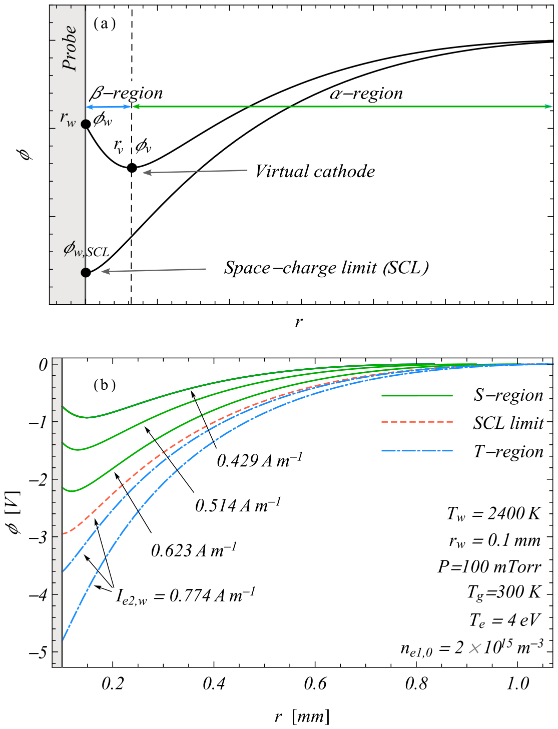
In particular, we show that, before the inverse sheath mode is reached, a new regime emerges in which ions are confined in the presheath, and the ion flux towards the surface vanishes. In this regime, the double-sheath structure associated with the virtual cathode is still present, as in the SCL regime. The transition to a fully developed inverse sheath occurs only when the potential at the bottom of the virtual cathode reaches the plasma potential. At this stage, the surface potential exceeds the plasma potential, leading to a monotonic potential profile across the sheath and a flat, non-accelerating profile in the presheath. Finally, we determine the variation of the floating potential with wall temperature and find a linear trend towards the plasma potential, consistent with the observations of Jilek Z. et al. [56]. The TL and SCL potential profiles, together with the $\alpha$/$\beta$-region notation used below, are summarised in Figure 1.

2. The Model

In the fluid model used here, a thermionic probe may be held at an arbitrary potential relative to the plasma. The plasma–probe interaction is described by the ion continuity and momentum equations, the latter also referred to here as the ion equation of motion [41,42]:

$$\begin{array}{ccc}\hfill & & {\left(r{n}_i{v}_i\right)}^{\prime }=r{\nu }_{iz}{n}_{e1},\hfill \end{array}$$

(1a)

$$\begin{array}{ccc}\hfill & & M{n}_i{v}_i{v}_i^{\prime }=-e{n}_i{\varphi }^{\prime }-{\nu }_{iz}M{n}_{e1}{v}_i-{\nu }_{c}M{n}_i{v}_i,\hfill \end{array}$$

(1b)

where r is the radial distance from the probe centre; a prime denotes differentiation with respect to r; M, $n_i$ and $v_i$ are the ion mass, density and velocity, respectively; $\varphi$ is the electric potential relative to the plasma potential; ${\nu }_{iz}$ is the ionisation frequency (only ionisation by plasma electrons is considered, because emitted electrons have a negligible ionisation rate coefficient); and ${\nu }_c$ is the ion–neutral collision frequency. The plasma-electron continuity and momentum equations are

$$\begin{array}{ccc}\hfill & & {\left(r{n}_{e1}{v}_{e1}\right)}^{\prime }=r{\nu }_{iz}{n}_{e1},\hfill \end{array}$$

(2a)

$$\begin{array}{ccc}\hfill & & m{n}_{e1}{v}_{e1}{v}_{e1}^{\prime }=e{n}_{e1}{\varphi }^{\prime }-{\nu }_{iz}m{n}_{e1}{v}_{e1}-n_{e1}^{\prime }{k}_B{T}_e,\hfill \end{array}$$

(2b)

where $T_e$ is the plasma-electron temperature; m is the electron mass; and $n_{e1}$ and $v_{e1}$ are the number density and velocity of the plasma electrons, respectively. Assuming that the emitted electrons are Maxwellian, they satisfy

$$\begin{array}{ccc}\hfill & & {\left(r{n}_{e2}{v}_{e2}\right)}^{\prime }=0,\hfill \end{array}$$

(3a)

$$\begin{array}{ccc}\hfill & & m{n}_{e2}{v}_{e2}{v}_{e2}^{\prime }=e{n}_{e2}{\varphi }^{\prime }-n_{e2}^{\prime }{k}_B{T}_w,\hfill \end{array}$$

(3b)

where $T_w$ is the probe temperature, and the subscript $e2$ denotes emitted electrons. Finally, Poisson’s equation is

$${\epsilon }_0{\left(r{\varphi }^{\prime }\right)}^{\prime }=-er(n_i-n_{e1}-n_{e2}).$$

(4)

To close the model, the following auxiliary equations are considered

$$\begin{array}{ccc}\hfill & & {\nu }_{iz}=K_{iz}{n}_g=22.59\times {10}^{11}{T}_e^{0.59}{e}^{-17.44/T_e}P/T_g,\hfill \end{array}$$

(5a)

$$\begin{array}{ccc}\hfill & & {\nu }_c={\sigma }_c{n}_g\left|v_i\right|=-9.65\times {10}^6{v}_{i}P/T_g,\hfill \end{array}$$

(5b)

$$\begin{array}{ccc}\hfill & & J_{RD}=A_{RD}{T}_w^2{e}^{-e{W}_f/k_B{T}_w},\hfill \end{array}$$

(5c)

$$\begin{array}{ccc}\hfill & & v_{e2,w}=\sqrt{2k_B{T}_w/\pi m}\hfill \end{array}$$

(5d)

In these expressions, $K_{iz}$ is given in ${\mathrm{m}}^3{\mathrm{s}}^{-1}$ [61,62], ${\nu }_{iz}$ and ${\nu }_c$ in ${\mathrm{s}}^{-1}$, the neutral gas pressure P in Torr, the neutral gas temperature $T_g$ in K, and the ion velocity $v_i$ in m/s. The electron temperature is given in eV and is taken in the range $T_e\sim$ 2–7 eV. The sign convention is such that ions moving towards the probe have $v_i<0$. Finally, $J_{RD}$ is the classical Richardson–Dushman thermionic emission current density, $W_f$ is the work function of the surface, and $v_{e2,w}$ is the emitted-electron velocity at the probe surface.

It is important to note that the model includes three independent presheath mechanisms—ionisation, ion–neutral collisions, and geometric compression—each characterised by its own length scale: ${\lambda }_{iz}=c_B/{\nu }_{iz}$, ${\lambda }_c=c_B/{\nu }_c$, and $r_w$ [63,64]. The actual presheath scale is determined by the minimum of these three lengths, $\lambda =\min \{{\lambda }_{iz},{\lambda }_c,r_w\}$. Consequently, depending on the experimental parameters, the presheath may be dominated by collisions, geometry, or ionisation. For the conditions considered here ($P=100$ mTorr, $r_w=0.1$ mm), the dominant scales are ${\lambda }_c$ and $r_w$, while ${\lambda }_{iz}$ is much larger. The model therefore remains fully valid even in the limit of negligible ionisation (${\nu }_{iz}\to 0$), where it reduces to a collisional/geometric presheath formulation.

The potential profile is obtained using a shooting method [41,42]. Rather than imposing the boundary condition at the probe surface directly, the method starts from a point $r=L$ in the presheath, where the quasineutrality condition $n_i=n_{e1}+n_{e2}$ holds, and varies L until the required surface condition is satisfied (see Appendix A). In this formulation, the model is solved on the semi-infinite physical domain $r\in [r_w,\infty )$. The point $r=L$ is chosen sufficiently far from the probe in the quasineutral plasma ($\varphi \approx -{10}^{-8}{k}_B{T}_e/e$) to serve as the starting point for the numerical integration. For $r\ge L$, the potential and density profiles are given by the quasineutral solution.

Operating the probe in the TL regime results in a probe potential below the plasma potential, with a monotonic potential profile that slows down the plasma electrons. In this case, (2a,b) reduce to the Boltzmann relation $n_{e1}=n_{e1,0}{e}^{\varphi /k_B{T}_e}$, where $n_{e1,0}$ is the electron density in the plasma. In contrast, when operating the probe within the SCL regime (Figure 1), a virtual cathode appears characterised by a non-monotonic potential profile, and the model is solved in two steps as detailed in Appendix A. As a first step, we obtain the electric potential profile $\varphi \left(r\right)$ in the $\alpha$-region (Figure 1), extending from the quasineutral plasma at $r=L$, where quasineutrality holds, up to the point where the electric field vanishes. This point defines the virtual cathode ’dip’, characterised by its location $r=r_v$ and potential value ${\varphi }_v$, which are determined by the condition ${\varphi }^{\prime }\left(r_v\right)=0$. Then, as a second step, we solve the model from $r=r_v$ to the probe surface $r=r_w$ (known as the $\beta$-region), in which the electric field is repulsive to the emitted electrons. As shown in Appendix A, Equations (3a,b) reduce in this region to

$$n_{e2}=n_{e2,v}{e}^{e(\varphi -{\varphi }_v)/k_B{T}_w}.$$

(6)

Finally, we repeat this two-step procedure successively while varying only the parameter L until the solution satisfies the following boundary condition on the probe surface

$$J_{e2,w}=J_{e2,v}{e}^{e({\varphi }_v-{\varphi }_w)/k_B{T}_e},$$

(7)

where $J_{e2,w}=J_{RD}\left(T_w\right)$, $J_{e2,v}=I_{e2,v}/2\pi r_v$ and $I_{e2,v}$ is the net emitted current per unit length overcoming the virtual cathode.

Thus, operating this way, for fixed values of $T_w$, P, $T_e$, and $r_w$, we can obtain the potential profile $\varphi$; the particle density profiles $n_i$, $n_{e1}$, and $n_{e2}$; the location of the virtual cathode $r_v$; the probe potential ${\varphi }_w$; and the net emitted current overcoming the virtual cathode $I_{e2,v}$. As shown in Appendix A, the virtual cathode potential ${\varphi }_v$ is therefore used below as an internal continuation parameter that labels self-consistent solutions of the shooting method, not as a directly imposed experimental control.

3. Results

In contrast to previous models [4,8,24], in this approach the probe potential ${\varphi }_w$ in the SCL regime is an output of the calculation, not an initially assumed value. This allows us to solve the plasma–surface interaction without assuming a priori that ${\varphi }_w$ must become positive, i.e., above the plasma potential, for an inverse sheath to form. The model can therefore describe how this interaction evolves from the TL regime to the IS regime as ${\varphi }_w$ changes from values below the plasma potential to values above it. This makes it possible to solve the plasma–wall interaction without assuming a specific sign for ${\varphi }_w$, thereby allowing us to study how this interaction transits from the TL regime to the IS regime.

Figure 1a sketches the $\alpha$ and $\beta$-regions of a probe working in the SCL regime, while Figure 1b represents some of the calculated potential profiles when it operates in both the TL and SCL regimes. For negative probe potentials far below the plasma potential, all emitted electrons reach the plasma, following an accelerating monotonic potential profile. In this regime, the emission is governed solely by the probe temperature, and the probe operates in the temperature-limited (TL) regime, also referred to as the T-region of the I–V characteristic curve (potential profiles depicted by the blue curves in Figure 1b). Unlike passive collecting probes, as the probe potential approaches the plasma potential (${\varphi }_w\to 0$), the electric field at the probe surface can vanish due to the presence of emitted electrons, marking the space-charge limit (SCL limit) (red curve in Figure 1b). Beyond this limit, for probe potentials even closer to the plasma potential, the electric field at the probe surface reverses its sign, resulting in the formation of a virtual cathode—a potential well in front of the probe. This non-monotonic potential structure is caused by the accumulation of negative charge near the probe, which reflects a fraction of the emitted electrons back to the probe. In this case, the emission is controlled by this accumulated charge. This regime is referred to as the space-charge-limited (SCL) regime, or the S-region (green curves in Figure 1b).

Using the aforementioned two-step method, we find that, in the SCL regime, as the model is solved for decreasing values of the net current emitted by the probe $I_{e2,w}$, the electric potential at the bottom of the potential well approaches the plasma potential, ${\varphi }_v\to 0$, and the accumulation of negative particles near the probe also increases [42]. This occurs due to the reduced acceleration with which emitted electrons are expelled into the plasma in the $\alpha$-region, the increased ability of plasma electrons to overcome the retarding potential, and the reduced attraction of ions towards the probe. This increase in negative charge near the surface deepens the virtual cathode potential, ${\varphi }_w-{\varphi }_v$, in the $\beta$-region, while simultaneously reducing the electric field in the $\alpha$-region. As a consequence of the reduced acceleration experienced by ions in the $\alpha$-region and the increased retardation in the $\beta$-region, a threshold value of the net current emitted by the probe $I_{e2,w}$, and therefore of the virtual cathode dip potential, ${\varphi }_v$, exists at which the ion velocity, $v_i$, at the probe surface vanishes. Beyond this threshold value, it becomes impossible to find a solution that satisfies the boundary condition (7), as the ion fluid loses its velocity before reaching the probe. This results in a mathematical singularity in the ion density within the fluid framework, as demonstrated by combining Equations (1a,b), signalling the breakdown of the fluid description at that location.

$$n_i^{\prime }=(e{M}^{-1}{n}_i{\varphi }^{\prime }+2{\nu }_{iz}{n}_{e1}{v}_i+{\nu }_c{n}_i{v}_i-n_i{v}_i^2{r}^{-1})/v_i$$

(8)

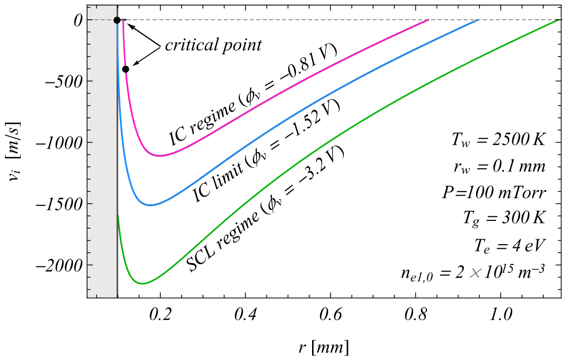
Figure 2 represents the ion velocity profile for three self-consistent solutions labelled by the virtual cathode dip ${\varphi }_v$. For ${\varphi }_v=-3.2\mathrm{V}$ (green curve in Figure 2), the probe operates in the SCL regime: positive ions reach the probe before their velocity $v_i$ vanishes, and it is possible to find a solution that fulfils (7). Continuing the solution family towards virtual cathode dips closer to the plasma potential (${\varphi }_v\to 0$), the threshold value ${\varphi }_v=-1.52\mathrm{V}$ is reached, at which $v_i$ vanishes exactly on the probe surface (blue curve). Beyond this threshold, the fluid ion velocity asymptotically approaches zero before the probe surface is reached. The resulting mathematical singularity ($n_i\to \infty$) makes it impossible to extend the fluid solution to the probe surface while fulfilling (7), indicating the emergence of a kinetically dominated layer. This means that beyond the threshold value ${\varphi }_v=-1.52\mathrm{V}$, a third region appears between the quasineutral plasma and the probe (which we refer to as the $\gamma$-region), which lacks ions, with the ions remaining confined to the $\alpha$ and $\beta$-regions. Beyond this threshold value, the plasma–wall interaction would be characterised by an ion-confinement (IC) regime and would still be compatible with the virtual cathode structure.

The mechanism causing this confinement is the increase in the potential depth of the virtual cathode ${\varphi }_w-{\varphi }_v$ as the probe potential approaches the plasma potential (${\varphi }_w\to 0$), as shown in Figure 1b and more clearly in Figures 5–7 of Ref. [42]. This increase slows down ions between $r_v$ and $r_w$ at a rate faster than the presheath can accelerate them from L to $r_v$. Consequently, as can be observed in Figure 2 for ${\varphi }_v=-0.81$ V, the macroscopic fluid ion velocity asymptotically approaches zero at a finite distance before the ions reach the probe, i.e., at a point located in front of the probe surface ($r>r_w$). This zero-velocity location is denoted as the critical point $r_c$. Rather than representing a physical accumulation of infinite density, this condition marks the position where the fluid approximation mathematically diverges and reaches its limit of validity. At this location, kinetic dominance begins, and phenomena such as ion trapping [54] would locally govern the potential. Therefore, we truncate the fluid solution at $r_c$ and treat the remaining space $r_c\to r_w$ as a transition layer ($\gamma$-region), reflecting the macroscopic onset of an inverse sheath structure as supported by kinetic simulations [26,33,56]. This point is found between the virtual cathode and the probe surface, i.e., $r_w<r_c<r_v$.

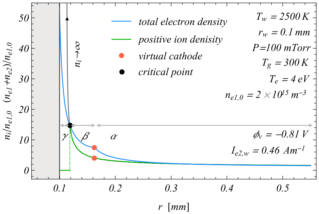
The net charge density is negative near the virtual cathode, but close to the confinement point $r_c$, the ion density $n_i$ rapidly grows and reaches the total electron density. To regularise the solution at the fluid breakdown point, we define $r_c$ operationally as the location where quasineutrality is recovered, i.e., $n_i=n_{e1}+n_{e2}$ (black circles in Figure 2, Figure 3 and Figure 4b). At this point, the directed ion flux towards the probe is assumed to vanish. By imposing zero ion flux (${\mathsf{\Gamma }}_i=0$) and truncating the fluid ion density beyond $r_c$, we obtain the modified Poisson Equation (9). Physically, this operational truncation acknowledges that while trapped ions may accumulate in the virtual cathode (altering the local microphysics via BGK-like structures [54]), their macroscopic directed flux to the probe is halted. The region $r_c\to r_w$ is thus treated macroscopically as an ion-depleted transition layer ($\gamma$-region), allowing the fluid model to bridge the gap to the inverse sheath without requiring a full kinetic resolution of the trapped particle phase-space.

Figure 3 represents the total electron density $n_{e1}+n_{e2}$ and the ion density $n_i$ for ${\varphi }_v=-0.81\mathrm{V}$. Close to the virtual cathode, the total electron density prevails over the ion density until the fluid breakdown point, where $n_i$ diverges mathematically (ascending branch).

Hence, in this new IC regime, valid for $r_w\le r\le r_c$ where the fluid equations no longer apply, the Poisson equation reduces to

$${\epsilon }_0{\left(r{\varphi }^{\prime }\right)}^{\prime }=er(n_{e1}+n_{e2})$$

(9)

where $n_{e1}$ is determined by (2a,b) and $n_{e2}$ by (6). The boundary conditions at $r_c$ are given by

$$\begin{array}{ccc}\hfill \varphi \left(r_c\right)={\varphi }_c,& & {\varphi }^{\prime }\left(r_c\right)={\varphi }_c^{\prime },\hfill \end{array}$$

(10)

$$\begin{array}{ccc}\hfill n_{e1}\left(r_c\right)=n_{e1,c},& & v_{e1}\left(r_c\right)=v_{e1,c},\hfill \end{array}$$

(11)

where the values ${\varphi }_c$, ${\varphi }_c^{\prime }$, $n_{e1,c}$ and $v_{e1,c}$ are obtained from the corresponding solution in the $\beta$-region.

The truncation of the fluid ion density at $r_c$ and the imposition of ${\mathsf{\Gamma }}_i=0$ for $r<r_c$ are the macroscopic fluid-model counterpart of kinetic ion trapping. It is analogous to the standard simplification made for electrons in a retarding electric field: when the electron velocity tends to zero, the kinetic terms in the momentum equation are neglected, yielding a Boltzmann-type equilibrium. In the cold-ion limit ($T_i=0$), the condition $v_i\to 0$ in the ion momentum equation leads to $n_i=0$, producing a step-front ion density profile. If ion thermal motion were included, the singularity would be regularised, and the ion density would decay smoothly as $n_i\propto \exp (-e\varphi /k_B{T}_i)$, as shown by Zhang et al. [23] for inverse sheaths with negative-ion emission.

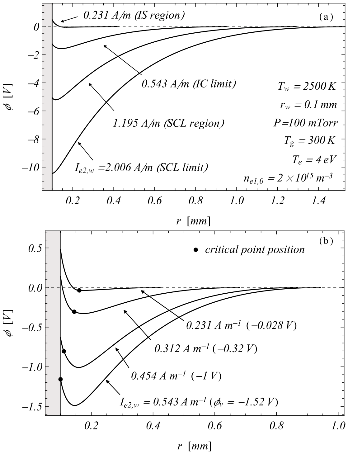
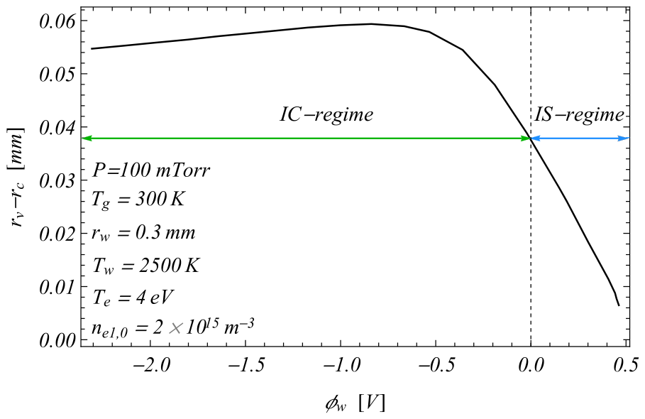
Figure 4a shows four potential profiles for different self-consistent values of ${\varphi }_v$ corresponding to: the SCL limit ($I_{e2,w}=2.006\mathrm{A}{\mathrm{m}}^{-1}$), for which the electric field vanishes at the probe surface and therefore ${\varphi }_w^{\prime }=0$ and $r_v=r_w$; the SCL regime ($I_{e2,w}=1.195\mathrm{A}{\mathrm{m}}^{-1}$), for which the electric field has changed sign at the probe surface, leading to the formation of a potential well in front of it and therefore $r_v>r_w$; the IC limit ($I_{e2,w}=0.543\mathrm{A}{\mathrm{m}}^{-1}$), for which the ion flux vanishes exactly at the probe surface and therefore $v_{i,w}=0$ and $r_c=r_w$; and finally, the case in which the inverse sheath regime is almost reached ($I_{e2,w}=0.231\mathrm{A}{\mathrm{m}}^{-1}$), for which ${\varphi }_v\to 0$ and $r_c\to r_v$. Figure 4b shows in more detail the variation of the potential profile when the probe operates within the IC regime, and illustrates how the transition from the SCL regime to the IS regime takes place. Here, we observe that (i) ion confinement and (ii) positive probe potential above the plasma potential, which characterise inverse sheaths, occur while a virtual cathode structure satisfying the boundary condition (7) is still present. When the virtual cathode minimum reaches the plasma potential ${\varphi }_v\to 0$, the fully developed inverse mode is finally reached. In this limit, the potential profile is monotonic, and the probe potential is above the plasma potential (${\varphi }_w>0$). The critical point then coincides with the virtual-cathode minimum, i.e., $r_c=r_v$ (see Figure 5 and the black circles in Figure 4b as they approach the virtual-cathode minimum). This implies that the $\alpha$-region (from L to $r_v$) remains as a quasineutral, flat-potential, non-accelerating region with no electric field; the $\beta$-region (from $r_v$ to $r_c$) disappears (Figure 5); and the $\gamma$-region (from $r_c$ to $r_w$) is an ion-free region that occupies the whole (inverse) sheath [26].

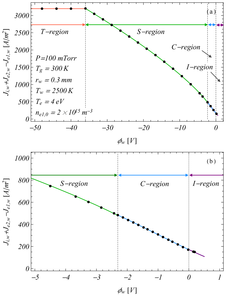
Figure 6 shows the I–V curve [42] for the probe operating in the TL regime (T-region), SCL regime (S-region), IC regime (C-region) and IS regime (I-region), as well as their corresponding fitted curves for the first three regimes.

When the probe operates in the TL regime, the whole thermionic emission current density, $J_{RD}$, reaches the plasma. In contrast, in the SCL and IC regimes, only the fraction of the emitted current that overcomes the virtual cathode reaches the plasma, namely $I_{e2,v}$ per unit axial length. The remaining current, $2\pi r_w{J}_{RD}-I_{e2,v}$, is reflected by the potential well and returns to the probe. The net current density collected by the probe in these three regimes is given by

$$J_w=J_{i,w}+J_{e2,w}-J_{e1,w}$$

(12)

where $J_{i,w}$, $J_{e2,w}$ and $J_{e1,w}$ are the ion, net emitted electron and plasma electron current densities at the probe surface, respectively. In the TL regime, these currents can be expressed as follows:

$$\begin{array}{ccc}& & J_{i,w}=-e{n}_{i,w}{v}_{i,w},\hfill \end{array}$$

(13a)

$$\begin{array}{ccc}& & J_{e2,w}=J_{RD},\hfill \end{array}$$

(13b)

$$\begin{array}{ccc}& & J_{e1,w}=e{n}_{e1,0}{e}^{e{\varphi }_w/k_B{T}_e}\sqrt{k_B{T}_e/2\pi m}\hfill \end{array}$$

(13c)

where $n_{i,w}=n_i\left(r_w\right)$ and $v_{i,w}=v_i\left(r_w\right)<0$ are obtained from the model solution. In the SCL regime, these same current densities can be determined from $n_{e1,w}=n_{e1}\left(r_w\right)$, $v_{e1,w}=v_{e1}\left(r_w\right)$, and $I_{e2,v}=2\pi r_{v}e{n}_{e2}\left(r_v\right)v_{e2}\left(r_v\right)$ (see Appendix A, Equation (A9a)), and are written as

$$\begin{array}{ccc}& & J_{i,w}=-e{n}_{i,w}{v}_{i,w},\hfill \end{array}$$

(14a)

$$\begin{array}{ccc}& & J_{e2,w}=I_{e2,v}/2\pi r_w,\hfill \end{array}$$

(14b)

$$\begin{array}{ccc}& & J_{e1,w}=-e{n}_{e1,w}{v}_{e1,w},\hfill \end{array}$$

(14c)

where $v_{i,w}<0$, $v_{e1,w}<0$ and $I_{e2,v}>0$. Finally, in the IC regime:

$$\begin{array}{ccc}& & J_{i,w}=0,\hfill \end{array}$$

(15a)

$$\begin{array}{ccc}& & J_{e2,w}=I_{e2,v}/2\pi r_w,\hfill \end{array}$$

(15b)

$$\begin{array}{ccc}& & J_{e1,w}=-e{n}_{e1,w}{v}_{e1,w},\hfill \end{array}$$

(15c)

where $v_{e1,w}<0$ and $I_{e2,v}>0$. For each probe temperature $T_w$, the corresponding fitted expressions for the three regimes are

$$\begin{array}{cc}{J}_w\left({\varphi }_w\right)=& a_0+a_1{e}^{e{\varphi }_w/k_B{T}_e}+c\sqrt{-e{\varphi }_w/k_B{T}_e},\hfill \end{array}$$

(16a)

$$\begin{array}{cc}{J}_w\left({\varphi }_w\right)=& a_0+a_1{e}^{e{\varphi }_w/k_B{T}_e}+c\sqrt{-e{\varphi }_w/k_B{T}_e}+a_3(-e{\varphi }_w/k_B{T}_e)+\hfill \\ & +a_4{(-e{\varphi }_w/k_B{T}_e)}^2,\hfill \end{array}$$

(16b)

$$\begin{array}{ccc}\hfill & J_w\left({\varphi }_w\right)=& a_0+a_1{e}^{e{\varphi }_w/k_B{T}_e}+a_3(-e{\varphi }_w/k_B{T}_e)+a_4{(-e{\varphi }_w/k_B{T}_e)}^2.\hfill \end{array}$$

(16c)

As has been experimentally observed by Yip C. S. et al. [65], Figure 6a shows an increase in the slope of the I–V characteristic as the probe potential approaches the plasma potential (${\varphi }_w\to 0$), which is related to the increase in the negative charge in the vicinity of the emitting surface. This is due to the ion-confinement regime, which reduces the saturation effect of the virtual cathode on the emitted current, leading to an increase in this current.

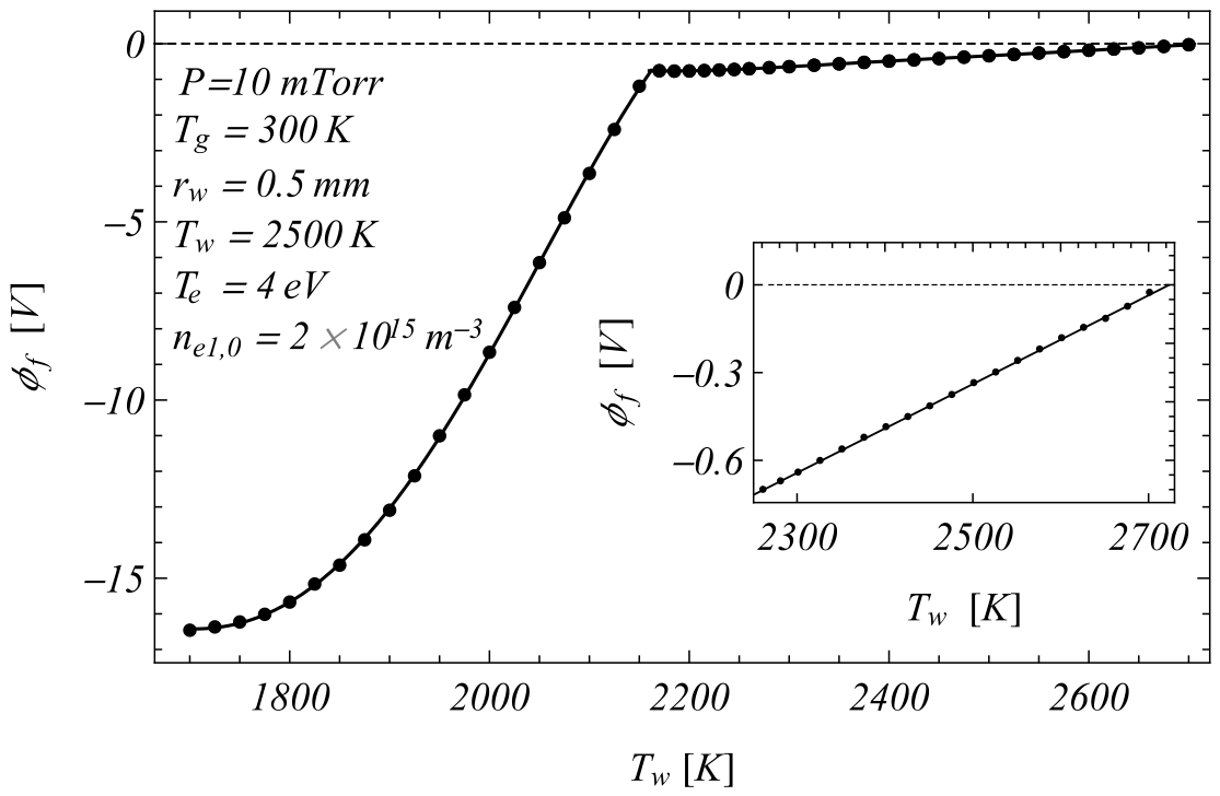
These numerical fits allow us to obtain the floating potential ${\varphi }_f$ for each value of $T_w$ by solving the equation $J_w\left({\varphi }_w\right)=0$. This floating condition corresponds to the particular case of a current-free emitting surface; any other point of the I–V characteristic describes the probe biased at the corresponding potential with respect to the plasma. Furthermore, Figure 7 shows the variation of ${\varphi }_f$ with $T_w$ for a probe of radius $r_w=0.5\mathrm{mm}$. In the range $T_w\sim 1700$–$2160\mathrm{K}$, the probe operates in the T-region and ${\varphi }_f$ is strongly affected by $T_w$. However, in the range $T_w\sim 2160$–$2270\mathrm{K}$, the probe operates in the SCL regime and ${\varphi }_f$ remains almost constant [42]. Finally, from $T_w=2300\mathrm{K}$, when the probe begins to operate in the IC regime, the floating potential gradually increases until it reaches values above the plasma potential within the IS regime (${\varphi }_w\sim 0.5\mathrm{V}$). As reported by Jilek Z. et al. [56], the inset in Figure 7 shows how ${\varphi }_f$ depends linearly on $T_w$ when the probe operates in the ion-confinement regime for $T_w\sim 2300$–$2700\mathrm{K}$ before reaching the plasma potential, the slope of the fit being $1.52\mathrm{mV}/\mathrm{K}$.

4. Limitations of the Fluid Approach and Kinetic Interpretation

While the fluid model accurately predicts macroscopic quantities (I–V curves and the floating potential) for T- and S-regimes [41,42], the ion-confinement (IC) regime pushes it to its theoretical boundary. The condition $v_i\left(r_c\right)\to 0$ leads to a mathematical singularity that physically corresponds to the onset of ion kinetic trapping. Recent kinetic studies [54] demonstrate that for deep virtual cathodes, trapped ion populations form BGK-like structures, effectively smoothing the potential well locally. In our fluid framework, we interpret the singular point as the boundary where kinetic corrections become essential. By imposing ${\mathsf{\Gamma }}_i=0$ for $r<r_c$, we bypass the microscopic resolution of the trapped-ion space charge and instead model the macroscopic consequence of ion confinement: the cessation of the directed ion beam towards the probe. This is conceptually similar to the step-front particle model used in canonical sheath theory to describe electron depletion inside positive-ion sheaths described by Sternberg and Godyak [66]. If ion thermal motion were retained, the step-front would be replaced by a smooth exponential decay $n_i\propto \exp (-e\varphi /k_B{T}_i)$, as demonstrated by Zhang et al. [23] for inverse sheaths with negative-ion emission. Thus, the IC regime is a physical feature of the transition to an inverse sheath, not an artefact of the cold-fluid approximation. This approach agrees with the results obtained by Jilek et al. [56], who performed PIC/MC simulations under conditions analogous to ours (cylindrical emissive probe, collisional argon presheath) and observed SCL potential profiles with a floating potential that increases linearly with $T_w$ before reaching the plasma potential, precisely the behaviour predicted by our fluid model (Figure 7, inset). Specifically, the predicted linear slope of the floating potential with temperature ($1.52$ mV/K) and the transition threshold ($T_w\sim 2300$ K for the parameters of Figure 7) are in quantitative agreement with the PIC/MC parameter scans reported by Jilek et al. (2022, Ref. [56]), where the SCL-to-IS transition occurs under analogous plasma conditions. Gyergyek et al. [58,59] further showed that fluid models can accurately predict macroscopic sheath quantities even when kinetic structures are locally present. Thus, the present model can be used to predict measurable quantities, such as ${\varphi }_f$ and I–V curves, in cases where fluid averaging over kinetic details is appropriate, as supported by the agreement with experimental trends [55,56]. It therefore describes a continuous transition pathway from SCL to IS via ion confinement, consistent with the parameter scans reported by Jilek et al. [56]. A full kinetic treatment resolving the detailed structure of the $\gamma$-region is beyond the scope of this work and will be addressed in future publications.

5. Conclusions

In conclusion, when the probe operates in the SCL regime, the potential drop in the virtual cathode ${\varphi }_w-{\varphi }_v$ increases as the probe potential approaches the plasma potential (${\varphi }_w\to 0$). This effect enhances ion deceleration in the $\beta$-region, from the virtual cathode to the probe surface ($r_v$ to $r_w$) as compared with the ion acceleration in the presheath from L to $r_v$. Therefore, ions eventually reach the limit of the fluid description ($v_i\to 0$) before reaching the probe, becoming effectively confined while the virtual cathode structure still exists. This fluid breakdown condition marks the transition to a kinetically dominated layer that we model as an ion-depleted $\gamma$-region.

This mechanism results in a steeper slope of the I–V curve close to the plasma potential, as reported by Yip et al. [65], and allows the floating potential to reach the plasma potential linearly even in an SCL sheath. This regime can help control plasma–surface interactions on highly emitting surfaces, mitigating sputtering and material erosion. Only when the minimum value of the virtual cathode reaches the plasma potential, i.e., ${\varphi }_v\to 0$, does the potential profile become monotonic within the sheath, with a non-accelerating presheath, meaning that the fully developed inverse sheath regime has been reached. Finally, we note that the ion-confinement pathway identified here provides a macroscopic criterion for the onset of kinetic trapping effects. While kinetic studies suggest that ionisation may destabilise the SCL sheath [26,29,30,31,33,34,54], our fluid model captures the continuous transition observed in PIC simulations [56], where the floating potential evolves linearly from the SCL saturation value towards the plasma potential.

References

1. Langmuir, I. The pressure effect and other phenomena in gaseous discharges. J. Frankl. Inst. B 1923, 196, 751–762. [Google Scholar] [CrossRef] [Scilit]
2. Langmuir, I. The Interaction of Electron and Positive Ion Space Charges in Cathode Sheaths. Phys. Rev. 1929, 33, 0954–0989. [Google Scholar] [CrossRef] [Scilit]
3. Tonks, L.; Langmuir, I. A General Theory of the Plasma of an Arc. Phys. Rev. 1929, 34, 0876–0922. [Google Scholar] [CrossRef] [Scilit]
4. Hobbs, G.D.; Wesson, J.A. Heat flow through a Langmuir sheath in the presence of electron emission. Plasma Phys. 1967, 9, 85. [Google Scholar] [CrossRef] [Scilit]
5. Robertson, S. Sheaths in laboratory and space plasmas. Plasma Phys. Control. Fusion 2013, 55, 093001. [Google Scholar] [CrossRef] [Scilit]
6. Yamada, H.; Murphree, D.L. Electrostatic Probe Measurements in a Collisionless Plasma Sheath. Phys. Fluids 1971, 14, 1120–1126. [Google Scholar] [CrossRef] [Scilit]
7. Oksuz, L.; Hershkowitz, N. First experimental measurements of the plasma potential throughout the presheath and sheath at a boundary in a weakly collisional plasma. Phys. Rev. Lett. 2002, 89, 145001. [Google Scholar] [CrossRef] [Scilit] [PubMed]
8. Cavalier, J.; Lemoine, N.; Bousselin, G.; Plihon, N.; Ledig, J. Strongly emissive plasma-facing material under space-charge limited regime: Application to emissive probes. Phys. Plasmas 2017, 24, 013506. [Google Scholar] [CrossRef] [Scilit]
9. Sheehan, J.P.; Raitses, Y.; Hershkowitz, N.; Kaganovich, I.; Fisch, N.J. A comparison of emissive probe techniques for electric potential measurements in a complex plasma. Phys. Plasmas 2011, 18, 073501. [Google Scholar] [CrossRef] [Scilit]
10. Kar, R.; Barve, S.A.; Chopade, S.S.; Das, A.K.; Patil, D.S. A possible explanation of the anomalous emissive probe behavior in a reactive RF plasma. Plasma Sources Sci. Technol. 2012, 21, 055009. [Google Scholar] [CrossRef] [Scilit]
11. Dorf, L.; Raitses, Y.; Fisch, N.J. Electrostatic probe apparatus for measurements in the near-anode region of Hall thrusters. Rev. Sci. Instrum. 2004, 75, 1255–1260. [Google Scholar] [CrossRef] [Scilit]
12. Raitses, Y.; Staack, D.; Keidar, M.; Fisch, N.J. Electron-wall interaction in Hall thrusters. Phys. Plasmas 2005, 12, 057104. [Google Scholar] [CrossRef] [Scilit]
13. Haas, J.M.; Gallimore, A.D. Internal plasma potential profiles in a laboratory-model Hall thruster. Phys. Plasmas 2001, 8, 652–660. [Google Scholar] [CrossRef] [Scilit]
14. Sheehan, J.P.; Hershkowitz, N. Emissive probes. Plasma Sources Sci. Technol. 2011, 20, 063001. [Google Scholar] [CrossRef] [Scilit]
15. Smith, J.R.; Hershkowitz, N.; Coakley, P. Inflection-point method of interpreting emissive probe characteristics. Rev. Sci. Instrum. 1979, 50, 210–218. [Google Scholar] [CrossRef] [Scilit] [PubMed]
16. Hershkowitz, N. How Langmuir probes work. In Plasma Diagnotics Discharge Parameters and Chemistry; Academic Press: London, UK, 1989; Chapter 4; pp. 113–183. [Google Scholar]
17. Gyergyek, T.; Kovacic, J.; Cercek, M. A Fluid Model of the Sheath Formation in Front of an Electron Emitting Electrode with Space Charge Limited Emission Immersed in a Plasma that Contains a One-Dimensional Mono-Energetic Electron Beam. Contrib. Plasma Phys. 2010, 50, 121–134. [Google Scholar] [CrossRef] [Scilit]
18. Komm, M.; Ratynskaia, S.; Tolias, P.; Cavalier, J.; Dejarnac, R.; Gunn, J.P.; Podolnik, A. On thermionic emission from plasma-facing components in tokamak-relevant conditions. Plasma Phys. Control. Fusion 2017, 59, 094002. [Google Scholar] [CrossRef] [Scilit]
19. Schrittwieser, R.; Ionita, C.; Balan, P.; Silva, C.; Figueiredo, H.; Varandas, C.A.F.; Rasmussen, J.J.; Naulin, V. Turbulence and transport measurements with cold and emissive probes in ISTTOK. Plasma Phys. Control. Fusion 2008, 50, 055004. [Google Scholar] [CrossRef] [Scilit]
20. Schrittwieser, R.; Adamek, J.; Balan, P.; Hron, M.; Ionita, C.; Jakubka, K.; Kryska, L.; Martines, E.; Stockel, J.; Tichy, M.; et al. Measurements with an emissive probe in the CASTOR tokamak. Plasma Phys. Control. Fusion 2002, 44, 567–578. [Google Scholar] [CrossRef] [Scilit]
21. Mahdizadeh, N.; Greiner, F.; Ramisch, M.; Stroth, U.; Guttenfelder, W.; Lechte, C.; Rahbarnia, K. Comparison of Langmuir and emissive probes as diagnostics for turbulence studies in the low-temperature plasma of the torsatron TJ-K. Plasma Phys. Control. Fusion 2005, 47, 569–579. [Google Scholar] [CrossRef] [Scilit]
22. Rizopoulou, N.; Robinson, A.P.L.; Coppins, M.; Bacharis, M. A kinetic study of the source–collector sheath system in a drifting plasma. Plasma Sources Sci. Technol. 2013, 22, 035003. [Google Scholar] [CrossRef] [Scilit]
23. Zhang, Z.; Wu, B.; Yang, S.L.; Zhang, Y.; Chen, D.Z.; Fan, M.W.; Jiang, W. Formation of stable inverse sheath in ion-ion plasma by strong negative ion emission. Plasma Sources Sci. Technol. 2018, 27, 06LT01. [Google Scholar] [CrossRef] [Scilit]
24. Schwager, L.A. Effects of secondary and thermionic electron emission on the collector and source sheaths of a finite ion temperature plasma using kinetic theory and numerical simulation. Phys. Fluids B-Plasma Phys. 1993, 5, 631–645. [Google Scholar] [CrossRef] [Scilit]
25. Campanell, M.D.; Khrabrov, A.V.; Kaganovich, I.D. Absence of Debye Sheaths due to Secondary Electron Emission. Phys. Rev. Lett. 2012, 108, 255001. [Google Scholar] [CrossRef] [Scilit] [PubMed]
26. Campanell, M.D. Negative plasma potential relative to electron-emitting surfaces. Phys. Rev. E 2013, 88, 033103. [Google Scholar] [CrossRef] [Scilit] [PubMed]
27. Sheehan, J.P.; Hershkowitz, N.; Kaganovich, I.D.; Wang, H.; Raitses, Y.; Barnat, E.V.; Weatherford, B.R.; Sydorenko, D. Kinetic Theory of Plasma Sheaths Surrounding Electron-Emitting Surfaces. Phys. Rev. Lett. 2013, 111, 075002. [Google Scholar] [CrossRef] [Scilit] [PubMed]
28. Rizopoulou, N.; Robinson, A.P.L.; Coppins, M.; Bacharis, M. Electron emission in a source-collector sheath system: A kinetic study. Phys. Plasmas 2014, 21, 103507. [Google Scholar] [CrossRef] [Scilit]
29. Campanell, M.D.; Umansky, M.V. Are two plasma equilibrium states possible when the emission coefficient exceeds unity? Phys. Plasmas 2017, 24, 057101. [Google Scholar] [CrossRef] [Scilit]
30. Campanell, M.D. Alternative model of space-charge-limited thermionic current flow through a plasma. Phys. Rev. E 2018, 97, 043207. [Google Scholar] [CrossRef] [Scilit] [PubMed]
31. Campanell, M.D.; Johnson, G.R. Thermionic Cooling of the Target Plasma to a Sub-eV Temperature. Phys. Rev. Lett. 2019, 122, 015003. [Google Scholar] [CrossRef] [Scilit] [PubMed]
32. Masline, R.; Smirnov, R.D.; Krasheninnikov, S.I. Influence of the inverse sheath on divertor plasma performance in tokamak edge plasma simulations. Contrib. Plasma Phys. 2020, 60, e201900097. [Google Scholar] [CrossRef] [Scilit]
33. Campanell, M.D. Possible mitigation of tokamak plasma-surface interactions using thermionic divertor plates with inverse sheaths. Phys. Plasmas 2020, 27, 042511. [Google Scholar] [CrossRef] [Scilit]
34. Johnson, G.R.; Campanell, M.D. Effects of emitting surfaces and trapped ions on the sheath physics and current flow in multidimensional plasma systems. Plasma Sources Sci. Technol. 2021, 30, 015003. [Google Scholar] [CrossRef] [Scilit]
35. Taccogna, F.; Longo, S.; Capitelli, M.; Schneider, R. Surface-driven asymmetry and instability in the acceleration region of Hall thruster. Contrib. Plasma Phys. 2008, 48, 375–386. [Google Scholar] [CrossRef] [Scilit]
36. Hatayama, A. Progress in modeling and numerical simulation of negative hydrogen ion sources (invited). Rev. Sci. Instrum. 2008, 79, 02B901. [Google Scholar] [CrossRef] [Scilit] [PubMed]
37. Wunderlich, D.; Gutser, R.; Fantz, U. PIC code for the plasma sheath in large caesiated RF sources for negative hydrogen ions. Plasma Sources Sci. Technol. 2009, 18, 045031. [Google Scholar] [CrossRef] [Scilit]
38. McAdams, R.; Bacal, M. The negative ion flux across a double sheath at the formation of a virtual cathode. Plasma Sources Sci. Technol. 2010, 19, 042001. [Google Scholar] [CrossRef] [Scilit]
39. Mochalskyy, S.; Lifschitz, A.F.; Minea, T. Extracted current saturation in negative ion sources. J. Appl. Phys. 2012, 111, 113303. [Google Scholar] [CrossRef] [Scilit]
40. Fubiani, G.; Boeuf, J.P. Three-dimensional modeling of a negative ion source with a magnetic filter: Impact of biasing the plasma electrode on the plasma asymmetry. Plasma Sources Sci. Technol. 2015, 24, 055001. [Google Scholar] [CrossRef] [Scilit]
41. Morales Crespo, R.; Muñoz Serrano, E.; Tejero-del Caz, A. Floating potential method using a thermionic emissive probe including an ionizing and collisional presheath. Plasma Sources Sci. Technol. 2022, 31, 095012. [Google Scholar] [CrossRef] [Scilit]
42. Morales Crespo, R.; Muñoz Serrano, E.; Tejero-del Caz, A. Analysis of the virtual cathode and floating potential of a thermionic emissive probe operating in the space-charge-limited regime. Plasma Sources Sci. Technol. 2023, 32, 065017. [Google Scholar] [CrossRef] [Scilit]
43. Ye, M.Y.; Takamura, S. Effect of space-charge limited emission on measurements of plasma potential using emissive probes. Phys. Plasmas 2000, 7, 3457–3463. [Google Scholar] [CrossRef] [Scilit]
44. Takamura, S.; Ohno, N.; Ye, M.Y.; Kuwabara, T. Space-Charge Limited Current from Plasma-Facing Material Surface. Contrib. Plasma Phys. 2004, 44, 126–137. [Google Scholar] [CrossRef] [Scilit]
45. Marek, A.; Jilek, M.; Pickova, I.; Kudrna, P.; Tichy, M.; Schrittwieser, R.; Ionita, C. Emissive Probe Diagnostics in Low Temperature Plasma—Effect of Space Charge and Variations of Electron Saturation Current. Contrib. Plasma Phys. 2008, 48, 491–496. [Google Scholar] [CrossRef] [Scilit]
46. Li, S.H.; Li, J.Q. Studies of virtual cathode characteristics near thermionic emission cathodes in a vacuum. Vacuum 2021, 192, 110496. [Google Scholar] [CrossRef] [Scilit]
47. Tierno, S.P.; Donoso, J.M.; Domenech-Garret, J.L.; Conde, L. Existence of a virtual cathode close to a strongly electron emissive wall in low density plasmas. Phys. Plasmas 2016, 23, 013503. [Google Scholar] [CrossRef] [Scilit]
48. Li, J.; Li, S. Calculation and error analysis of virtual cathode caused by a thermionic cathode. J. Appl. Phys. 2024, 136, 105105. [Google Scholar] [CrossRef] [Scilit]
49. Li, J.; Li, S.; Ma, H. Investigation of virtual cathode generated by a tungsten emissive probe in a vacuum. Phys. Scr. 2024, 99, 055974. [Google Scholar] [CrossRef] [Scilit]
50. Makowski, M.A.; Emmert, G.A. New method to measure plasma potential with emissive probes. Rev. Sci. Instrum. 1983, 54, 830–836. [Google Scholar] [CrossRef] [Scilit]
51. Bradley, J.W.; Thompson, S.; Gonzalvo, Y.A. Measurement of the plasma potential in a magnetron discharge and the prediction of the electron drift speeds. Plasma Sources Sci. Technol. 2001, 10, 490–501. [Google Scholar] [CrossRef] [Scilit]
52. Campanell, M.D.; Umansky, M.V. Strongly Emitting Surfaces Unable to Float below Plasma Potential. Phys. Rev. Lett. 2016, 116, 085003. [Google Scholar] [CrossRef] [Scilit] [PubMed]
53. Campanell, M.D.; Umansky, M.V. Improved understanding of the hot cathode current modes and mode transitions. Plasma Sources Sci. Technol. 2017, 26, 124002. [Google Scholar] [CrossRef] [Scilit]
54. Johnson, G.R.; Campanell, M.D. Analysis of the Transition Time between the Space-Charge-Limited and Inverse Regimes. Plasma Phys. Rep. 2019, 45, 69–85. [Google Scholar] [CrossRef] [Scilit]
55. Kraus, B.F.; Raitses, Y. Floating potential of emitting surfaces in plasmas with respect to the space potential. Phys. Plasmas 2018, 25, 030701. [Google Scholar] [CrossRef] [Scilit]
56. Jilek, Z.; Caloud, J.; Zikan, P.; Obrusnik, A.; Trunec, D. PIC/MC calculation of current-voltage characteristic of emissive probe. Plasma Sources Sci. Technol. 2022, 31, 035014. [Google Scholar] [CrossRef] [Scilit]
57. Gomez, I.; Valic, A.; Gyergyek, T.; Costea, S.; Kovacic, J. Particle-in-cell simulations of an inverted sheath. J. Phys. Conf. Ser. 2020, 1492, 012004. [Google Scholar] [CrossRef] [Scilit]
58. Gyergyek, T.; Kovacic, J.; Gomez, I.; Gunn, J.P.; Costea, S.; Mozetic, M. Kinetic model of an inverted sheath in a bounded plasma system. Phys. Plasmas 2020, 27, 023520. [Google Scholar] [CrossRef] [Scilit]
59. Gyergyek, T.; Costea, S.; Bajt, K.; Valic, A.; Kovacic, J. Formation of an inverted sheath in a one-dimensional bounded plasma system studied by particle-in-cell simulation. Phys. Plasmas 2021, 28, 123507. [Google Scholar] [CrossRef] [Scilit]
60. Masline, R.; Smirnov, R.D.; Krasheninnikov, S.I. Simulations of divertor plasmas with inverse sheaths. Phys. Plasmas 2020, 27, 092505. [Google Scholar] [CrossRef] [Scilit]
61. Lieberman, M.A.; Lichtenberg, A.J. Principles of Plasma Discharges and Materials Processing, 2nd ed.; John Wiley & Sons, Inc.: Hoboken, NJ, USA, 2005; pp. 1–757. [Google Scholar]
62. Gudmundsson, J.T.; Thorsteinsson, E.G. Oxygen discharges diluted with argon: Dissociation processes. Plasma Sources Sci. Technol. 2007, 16, 399–412. [Google Scholar] [CrossRef] [Scilit]
63. Morales Crespo, R. Complete parametrization of the plasma-sheath transition andI–Vcurves for a cylindrical or spherical Langmuir probe according to the features of the probe, simultaneously including geometry, ionization and collisions. Plasma Sources Sci. Technol. 2015, 24, 045012. [Google Scholar] [CrossRef] [Scilit]
64. Riemann, K.U. The Bohm criterion and sheath formation. J. Phys. D-Appl. Phys. 1991, 24, 493–518. [Google Scholar] [CrossRef] [Scilit]
65. Yip, C.S.; Jin, C.Y.; Zhang, W.; Xu, G.S.; Hershkowitz, N. Experimental investigation of sheath effects on I–V traces of strongly electron emitting probes. Plasma Sources Sci. Technol. 2020, 29, 025025. [Google Scholar] [CrossRef] [Scilit]
66. Sternberg, N.; Godyak, V.A. Approximation of the bounded plasma problem by the plasma and the sheath models. Phys. D 1996, 97, 498–508. [Google Scholar] [CrossRef] [Scilit]
Figure 1. (a) Illustration of the α and β -regions. (b) Different potential profiles for constant values of T w , r w , P, T g , T e , n e 1 , 0 and different values of ϕ w in the temperature-limited (TL) and space-charge-limited (SCL) regimes, labelled with the net current emitted by the probe I e 2 , w according to Ref. [42].
Plasma 09 00029 g001
Figure 2. Positive-ion velocity v i in the SCL regime, at the ion-confinement limit (IC limit), where v i vanishes at the probe surface, and in the ion-confinement (IC) regime, where v i = 0 before ions reach the probe.
Plasma 09 00029 g002
Figure 3. Ion and electron density profiles in the IC regime. Close to the critical point, the ion density n i reaches the singularity.
Plasma 09 00029 g003
Figure 4. (a) Potential profile for the transition from the SCL limit to the fully developed inverse sheath regime. (b) Potential profiles when the probe operates within the IC regime. The black circles represent the locations of the critical points.
Plasma 09 00029 g004
Figure 5. Variation of the β -region extent, defined as the distance from the virtual cathode r v to the critical point r c .
Plasma 09 00029 g005
Figure 6. (a) The current–voltage (IV) curve of an emitting probe working with different regimes. (b) Details of the C- and I-regions of this characteristic curve.
Plasma 09 00029 g006
Figure 7. Variation of the floating potential with the probe temperature.
Plasma 09 00029 g007
Disclaimer/Publisher’s Note: The statements, opinions and data contained in all publications are solely those of the individual author(s) and contributor(s) and not of MDPI and/or the editor(s). MDPI and/or the editor(s) disclaim responsibility for any injury to people or property resulting from any ideas, methods, instructions or products referred to in the content.