Abstract
A system-level study of a NOx abatement process by means of non-thermal plasma (NTP) generated with dielectric barrier discharges (DBDs) is the framework of this article. With the goal of system improvement, the kinetic reaction simulation software ZdPlaskin is considered to select the most favorable operating conditions in order to optimize NOx abatement (deNOx). A parametric exploration of the performance, through variations in operating conditions (temperature, power injection pattern, and input gas mixture composition), requires highly numerous simulations; thus, the shortest possible computation times with robust results are of significant interest. As such, an analysis and filtering method is proposed and detailed to build a minimized chemical kinetic reaction set, allowing us to reliably analyze the impact of the selected operating conditions for the DBD reactor on treatment performance.
1. Introduction
Nitrogen oxide (NOx) emissions represent serious environmental and health challenges, driving the development of advanced mitigation technologies [1,2,3,4]. Among these, non-thermal plasma (NTP) systems—especially dielectric barrier discharge (DBD [5,6,7,8]) reactors—have shown considerable potential for NOx removal. Our research aims to examine, at the system level, how various physical parameters—including electrical, thermal, fluid dynamic, and geometric factors—affect the efficiency of NOx abatement [9,10].
Our study is supported by experimental measurements and diagnoses which validate the couplings highlighted in the system. In this context, a test bench [2,10], presented in Section 2.1, has been designed, allowing for various analyses to be performed.
In order to predict NOx abatement performance—which is derived from the electrical power injection into the NTP—and to investigate the chemical reactions taking place in the reactor, we use ZdPlaskin. This dedicated simulation tool [11,12] allows us to consider the various excited species and their characteristic reactions compiled in databases that are available worldwide [13,14,15]. Other approaches for plasma-assisted chemistry simulations can be found in the literature [14,16,17,18,19]. Using the data retrieved from these databases without any modification leads to large kinetic models, which include all the publicly available knowledge about the species and the reactions taking place in the NTP. However, it also leads to relatively long simulation times, which make the planned optimization approach a rather unrealistic solution for improving the NOx abatement process. To address this issue, we have developed a method to reduce the number of species and reactions considered in the model. The ZdPlaskin tool and its configuration, as well as the reaction set reduction approach, are detailed in Section 2.2 and Section 2.3. The performance of the minimized reaction sets and the evaluation of their robustness are analyzed and discussed in Section 3 and Section 4.
2. Materials and Methods
2.1. Experimental Setup
The “deNOx” test bench was developed [2,10] at LAPLACE laboratory to support our experimental investigations; the schematic diagram of the experimental setup is presented in Figure 1. The system includes a DBD reactor, a gas blending system, a power supply, measurement instruments, and the control interface:
- The reactor has a coaxial cylindrical geometry made of quartz. The inner electrode is stainless-steel foil, and the outer electrode is a metallic mesh (knitted thin wires made of tinned copper) wrapped around the quartz tube. The length of the mesh is 77 mm. Detailed dimensions are shown in Figure 1.
- The treated gas mixture is composed of , and and flows through the DBD reactor. The gas composition and total flow rate are adjustable: mass flow controllers (Bronkhorst EL-FLOW Prestige) are used to measure and regulate them. This mixture is intended to support research into the use of hydrogen in burners or combustion engines. It also allows for a comparison of the solutions and performance obtained in numerous studies available in the literature [1,2,3,4,5,6,7,9].
 Figure 1. Experimental setup and reactor dimensions.Figure 1. Experimental setup and reactor dimensions.
- The DBD voltage is measured with a 200 MHz digital oscilloscope (LeCroy HDO4024) connected through a 1000:1 voltage probe (Testec TT-SI 9010), and the current is measured using a current probe (LeCroy AP015). Gas analyzers (Testo 350 and Serinus 40, specifically for low NOx concentrations) measure the and concentrations.
- A specific power supply [20,21] was developed to ignite the plasma and control the energy injected into the NTP. It delivers square current waveforms, as shown in Figure 2. This circuit integrates a DC current source connected in cascade with a full-bridge current inverter and a step-up transformer. The converter delivers current pulses, whose rectangular shape is controlled by three degrees of freedom, namely frequency , current amplitude , and pulse duration (, being the duty cycle in the range of 5–95%). The maximum current delivered by the current source (primary side of the transformer) is 12 A. The high-voltage transformer is designed to withstand a maximum voltage of 11 kV; its turn ratio is 11. The frequency can be varied from 80 kHz to 200 kHz.
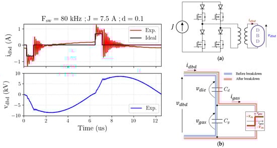 Figure 2. Square current source: synoptic (a) and electrical waveforms (vDBD in blue and iDBD in red). Here, Fsw = 80 kHz, J = 7.5 A, and d = 10%—DBD reactor equivalent circuit (b).
In order to control the increase in reactor temperature, this supply is operated in “Burst mode” [2,10]: pulses trains ( pulses) are separated by power injection pauses ( periods with inhibited pulses); the lengths of both bursts and pauses are fully controlled.
The whole bench is controlled and monitored by a supervisor developed in Labview, which
- Defines the configuration of each device;
- Defines the set point of controlled devices (mass flow controllers, power supply);
- Sets up and monitors batch experiments (gas mixtures, power supply control);
- Monitors data acquisition and measurement storage (database);
- Prepares measurements for post-treatment analyses.
The experimental operating conditions were carefully selected in order to obtain plasma that uniformly covers the reactor’s entire surface. This plasma is assumed to present a uniform spatial repartition. Assuming Townsend’s regime (which was subsequently verified), the classic equivalent circuit of the DBD (shown in Figure 2b) proves to be a very useful tool for simulated studies, as well as for identifying gas-related electrical quantities that cannot be measured experimentally [22,23].
2.2. System-Level Analysis and Kinetics of Plasma Gas Treatment
To analyze the chemical aspects of the process, ZdPlaskin software was selected. ZdPlaskin is a zero-dimensional plasma kinetics solver developed at LAPLACE laboratory [11]. Among other outcomes, it computes the evolution over time of species densities in non-thermal plasmas on the basis of a user-defined chemical reaction set (this set can be changed in order to study various NTP-induced chemical processes). ZdPlaskin includes BOLSIG+ [12], a Boltzmann equation solver mainly used to calculate rate coefficients for electron impact processes. As depicted in Figure 3, ZdPlaskin requires a kinetic mechanism description (a “kinet file”) that specifies the chemical species, the list of reactions, and the corresponding reaction rate coefficients (the reaction rate coefficient is the speed at which a chemical reaction takes place, defined as being proportional to the increase in the concentration of a product per unit time and to the decrease in the concentration of a reactant per unit time. The proportionality factors are the stoichiometric coefficients). These reaction rate coefficients define the dynamics of the changes in the concentration of the species, and they depend on the type of reaction:
- For gas-phase reactions, rate coefficients can be constant or temperature-dependent, often following an Arrhenius-type law.
- For electron impact reactions, rate coefficients depend on the electron collision cross-sections (cross-sections are a measure of the probability that a specific process will take place in a collision of two particles). Since the cross-sections also vary with electron energy, ZdPlaskin first calls BOLSIG+ to solve the electron energy distribution function (EEDF) and then computes the rate coefficients accordingly. The required cross-section data are sourced from LXCat, an open access, community-driven database for electron scattering cross-sections [13,14,15]. It should be noted that these databases are also used by commercial simulation products (for example, Comsol).

Figure 3.
ZdPlaskin input–output data flow.
Figure 3.
ZdPlaskin input–output data flow.

With the gas mixture () presented in the previous section, the NOx treatment is the result of two concurrent paths:
- Favorable reduction, which transforms into ;
- Unfavorable oxidation, which increases the amount.
The most important gas-phase reactions of both paths are presented in Table 1; the electron impact reactions (marked with ‘+++’ on the left) are presented as a single general form without detailing the numerous different excited states which can be produced.

Table 1.
Concurrent chemical paths.
The input variables (presented on the left in Figure 3) are used by ZdPlaskin to compute the reaction rates in order to predict the time variations in the various species, as will be explained in the next sections. As shown in Table 1, the electron impact reactions (marked with ‘+++’ on the left) producing excited species ( and ) present a reaction rate that depends on the reduced electric field . This time-varying quantity is evaluated as follows:
- The electric field is obtained from the voltage divided by the gap length. However, is not a directly measurable quantity (due to dielectric barriers in the reactor being present). With the records of and being measurements or simulation results, the evaluation of is straightforward [20] using the classical Equation (1) for the DBD:where is the equivalent capacitance of the dielectric barriers in the reactor, as shown in Figure 2b. It is worth mentioning in this context that the DBD device is represented by an equivalent lumped parameter circuit [21]. Experimental records are used to identify the parameters of this circuit on the basis of the Manley diagram [22,23]. This equivalent circuit is also useful to build the gas current waveform from the DBD voltage and current, and . Uniform behavior of the plasma is assumed, and no local phenomena (micro discharges, for instance, streamers) can be individually considered; this is in good agreement with the “zero dimensional” characteristic of the ZdPlaskin solver.
- The temperature is assumed to be uniform within the reactor. The gas number density is also uniform, being closely related to —according to the ideal gases law, one can state thatwhere is the Avogadro constant, is the ideal gas constant, and is the gas pressure (1 atm, constant in our case).
- The gas current is used together with the electric field to calculate the electron density necessary for electron impact reactions.
2.2.1. Modeling Equations
The essentials of ZdPlaskin software, which aims to solve equations that translate chemical reactions, are described below. For example, consider the generic reaction j:
, , and are chemical species, and , , , and are their stoichiometric coefficients within reaction j. The reaction rate of reaction j, is expressed as
and are the concentrations of species and , while is the reaction rate coefficient. may follow an Arrhenius-type law in the case of thermal gas-phase reactions or be computed by BOLSIG+ for electron impact reactions. In the framework of reaction j, the concentration of each involved species varies with its own variation’s rate given by (consumed reactants are associated with a minus sign, and products with a plus sign)
Considering all the species and chemical reactions listed in its “kinet file” associated with the process, according to Equations (4) and (5), ZdPlaskin builds a whole set of ordinary first-order differential nonlinear equations, as shown in Equation (6). In this equation, denotes the density of species, while represents the net production (or consumption) rate of species caused by reaction j. The right-hand side of (6) accounts for the sum of all contributions from all reactions (index j) involving species .
2.2.2. Equation Solving
ZdPlaskin numerically integrates Equation (6) and computes the time evolution of species densities. It achieves this integration using an explicit Euler method with a first-order time-stepping scheme. The simulation is typically carried out over a duration equal to , which is the residence time of the gas within the plasma reactor: is the average time available for chemical transformations to occur as the gas flows through the discharge region.
Evaluating the residence time might require relatively complex analysis [10,29,30]: indeed, the duration that the gas remains within the plasma reactor depends on its flow velocity, which in turn is influenced by the gas temperature. As the temperature increases, the gas density decreases (according to the ideal gas law), leading to an increase in the gas velocity in order to fulfill mass flow conservation. Since the temperature is generally non-uniform along the reactor, the gas velocity also varies with position. The residence time is therefore computed (7) by integrating the inverse of the local gas velocity over the reactor’s length :
For the results provided in this paper, these multi-physics couplings [10] are not developed, and the value of the residence time is considered an adjustable parameter for the simulations in ZdPlaskin.
2.2.3. Simulation Results and Performance
The creators of ZdPlaskin provide a comprehensive, ready-to-use “kinet file” with a reaction set for N2–O2 mixtures [31,32], comprising 53 chemical species and 656 reactions. Although extensive, this dataset is generic and was not specifically developed for investigating NOx reduction mechanisms. Following their recommendations, the SIGLO [13,14,15] database was used for and and the Phelps [13,14,33] database for .
Figure 4 and Figure 5 show time responses of NOx species and presents typical results obtained with ZdPlaskin; the x-axis is labeled “simulation time” in order to clearly differentiate it from experimental readings (where the x-axis is labeled “time”)—in both cases, it refers to the same time variable. Input gas mixtures are different: the first one is with , while the second is with . These results are based on the NTP chemistry scheme mentioned above [31,32] (53 different species and 656 reactions), which we named the “original kinetic mechanism” (OKM). According to the gas flow and reactor size, combined with temperature conditions (450 K, assumed uniform in the reactor), the residence time is 180 ms.
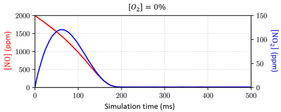
Figure 4.
ZdPlaskin outputs: time response of the decrease in NOx [] and [] without .
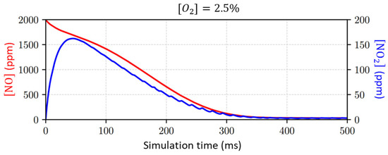
Figure 5.
ZdPlaskin outputs: time response of the decrease in NOx [] and [] with .
Simulating the whole equation set, solved over , takes 500 s on an AMD Ryzen 7 processor laptop (clock frequency 2.0 GHz, 16Go RAM).
Figure 6 shows an abacus obtained from a scan of the value. The comparison with experimental measurements opens up some very interesting prospects, allowing ZdPlaskin simulations to be considered a reliable alternative to long and costly experimental campaigns.
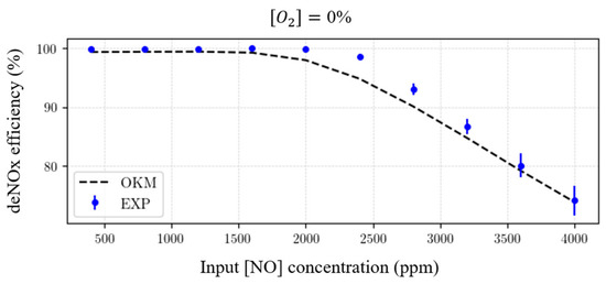
Figure 6.
ZdPlaskin outputs: performed sweep; varying the concentration highlights the variation in the performance of the deNOx process.
Nevertheless, given the time required to simulate a single given operating condition (500 s), constructing an abacus such as the one in Figure 6 is extremely tedious. With this in mind, the next subsection details the main contribution of this article, namely a method that aims to reduce the size of the NTP chemical scheme (number of species and reactions): this reduction is expected to reduce the simulation time while maintaining accurate results for analyses focused on NTP NOx reduction treatments.
2.3. Minimization of the Reaction Set for Kinetics Modeling
To target the relevant chemical species that mainly control the evolution of the deNOx process, we introduce the concept of “species of interest” (SOI): the latter are selected because they are considered prominent with respect to evaluating process performance. To select the additional species to be considered together with the species of interest and the minimal set of reactions to be associated with them for a consistent kinetic mechanism, our approach is based on
- Using the “original kinetic mechanism” (OKM) as the reference (in our case, it includes species and reactions). Indeed, this OKM has shown to very accurately reflect the experimental measurements (see Figure 6). Each tentative reduced kinetic mechanism will be compared to the later one (OKM);
- Proceeding with a two-step approach to build a “reduced kinetic mechanism” (RKM), as described below. The construction of the RKM, as well as the scans presented in Section 3 for robustness analysis, were performed using a toolkit called “Zukini,” developed by A. Cuellar.
2.3.1. First Step: Chemical Analysis-Based Selection of an “Initial Kinetic Mechanism”
In this study, we use the “stochiometric matrix” built by ZdPlaskin to mathematically translate the set of species ( is the number of species in OKM) and the set of reactions ( is the number of reactions in OKM) incorporated into its “kinet file”: in this matrix, each reaction is translated into a column and each line is associated with a species; the terms of each column are the stochiometric coefficients introduced in Equation (3) (with a positive sign for a “product” of the reaction (right hand side) or a negative sign if the “reactant” is consumed (left hand side). A value of 0 occurs when a species does not take part in the reaction).
An iterative inspection starting from the species of interest (SOI) is achieved, as shown in Figure 7. This enables the selection of reactions that produce or consume these species; then, the other species (not SOI) involved in these reactions are added to the species of interest, and again, the connected reactions are added. This simple process is repeated until the last iteration does not change the species set or the reaction set: these two sets are building the “initial kinetic mechanism” (IKM), which can be depicted as the chemical reaction network (CRN) or “reaction dependency graph” [34].
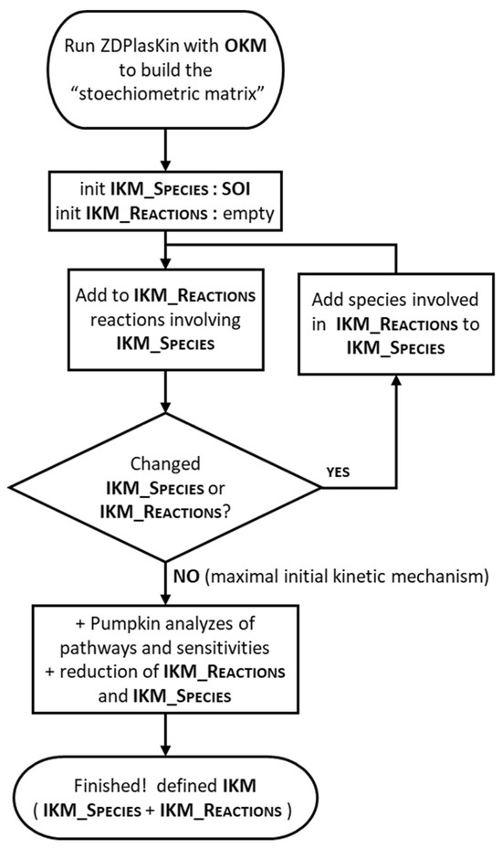
Figure 7.
Chemical analysis-based initial kinetic mechanism (IKM)—implemented algorithm.
The size of this initial kinetic mechanism is then reduced using the Pumpkin open access analysis tool [35]. Starting from the simulation results of ZdPlaskin, Pumpkin analyzes the variations in the products due to each reaction during the residence time. Among its settings, Pumpkin allows the user to select the number of pathways (chained chemical reactions) to be explored and specify the minimal participation percentage for the SOI which should be achieved by the selected pathways; on this basis, Pumpkin is able to select the reactions which contribute to the final products: these are kept in the IKM, and the others are discarded; accordingly, species which became irrelevant because they are disconnected from any reactions are also discarded.
It is important to mention that this reduction in the IKM introduces a risk of increasing the stiffness of the equation system (Equation (4)): indeed, intermediate reactions in a chain may have been arbitrarily eliminated. In this case, a size reduction in system (4) is often ineffective (from the point of view of simulation time performance), as solving stiff equations is generally slower. This is the reasoning behind the next step, which aims to ensure the numerical stability and completeness of the IKM, as described in Section 2.3.2.
2.3.2. Second Step: Numerical Stability and Completeness Approach
The aim of this second step is to add reactions and species to the initial kinetic mechanism to create a usable “kinet file”, which will guarantee numerical stability (avoiding the issues mentioned at the end of the previous section) and the speed of the simulations achieved by ZdPlaskin. Of course, at least concerning the species of interest, this new (hopefully reduced and faster for simulations) kinetic mechanism is expected to provide results similar to the ones obtained with the original kinetic mechanism.
As such, the following approach is developed, considering the species and the reactions belonging to the OKM that were not selected in the IKM obtained after the first step (this set is named “remainder” in Figure 8):
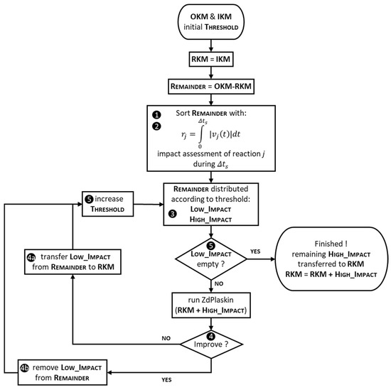
Figure 8.
Second step (completeness and numerical stability)—implemented algorithm. Numbers highlighted in the steps of the procedure denote the schedule’s items described below.
Once again, as shown in Figure 8, the process is iterative:
- Each reaction j in the “remainder” set is given an individual score, which is calculated as the integral of its reaction rate (as defined in Equation (4); the absolute value is considered) over the residence time . The reaction rate generally varies during the simulation; it is computed by ZdPlaskin running the OKM (each one of the reactions rates can be plotted among the curves built by ZdPlaskin). These scores translate the assessment of the impact of each reaction into a single figure based on the variation in the concentrations of products and reactants resulting from that reaction.
- All the reactions are sorted according to their score.
- A threshold level is introduced and reactions with higher scores than the threshold (reactions with “high impact”), together with their reactants and products, are used together with the “initial sets” (IKM) to build a new “kinet file”, which is then run with ZdPlaskin; other reactions (with scores below the threshold, considered as a “low impact” subset) are temporarily discarded.
- If the simulation time is longer than the simulation time of the previous iteration (or the one obtained with the OKM for the first iteration) or if the obtained time profiles of the species of interest differ too much from the OKM’s ones (more than 10% has appeared to be at a good level), then we consider that the attempt associated with the current threshold has failed:
- The temporarily eliminated reactions (“low impact” subset described at step 3) are thus considered necessary for a coherent description of the kinetic mechanism and are added, together with their associated species, to the “initial kinetic mechanism” (4a).
- If the attempt succeeds (both previous conditions are fulfilled), the temporarily discarded reactions and species are definitively eliminated (4b). It is worth mentioning at this step that the elimination process, which uses simulation results to check the relevancy of a kinetic reduction attempt, is in fact tightly bounded to the operating condition selected for the test (in some manner, it is similar to the “local linearization” of a nonlinear system, which is achieved in the vicinity of a given operating point)—see Table 4 below in the Section 3.
- The process is repeated with a higher threshold level until no reaction is left for potential elimination (“low impact” subset is empty).
- The result of these iterations is a reduced kinetic mechanism (RKM) focusing on the species that are initially selected among the species of interest (SOI).
3. Results
3.1. Performance of the Reduced Kinetic Mechanisms (RKM1 and RKM2)
The filtering process presented in the two subsections above (Section 2.3.1 and Section 2.3.2) was applied to two different sets of species of interest (SOI). Table 2 highlights the reduction in the size of the kinetic mechanisms and the drastic improvement in the simulation time using ZdPlaskin over the same residence time .
Table 2.
Reduced kinetic mechanism focusing on different sets of species of interest.
It is important to mention the size of the intermediate kinetic mechanisms obtained after the first step. The comparison with the sizes of RKM1 and RKM2 given in Table 2 highlights the impact of the second step (Section 2.3.2):
- For {, } SOI, IKM incorporates 189 reactions and 11 species to be compared with RKM1;
- For {, , , } SOI, IKM incorporates 374 reactions and 24 species to be compared with RKM2;
All species ultimately involved in the three kinetic mechanisms (OKM, RKM1, RKM2) are detailed in Table 3. It can be noted that the decrease in the number of species considered by the reduced kinetic mechanisms RKM1 and RKM2 (56 and 66) is not very significant compared to the original mechanism (68). The difference only concerns excited electronic states, while vibrational states are always retained, as are neutrals and ions.
Table 3.
Species used in the three kinetic mechanisms (OKM, RKM1, and RKM2).
The differences obtained in simulation times (last column of Table 2) are mainly due to the reduction in the number of chemical reactions (Table 2); this reduction is much greater than that of chemical species, which significantly reduces the time-step evaluation cost (Equation (6)).
The selected operating conditions used for testing the kinetic mechanisms (Table 2) are summarized in Table 4—these conditions were also used during the second step of the kinetic mechanism reduction.
Table 4.
Selected operating conditions.
3.2. Compared Time Responses of the Kinetic Mechanisms
As an example, Figure 9 and Figure 10 highlight the transient time responses for the species of interest, as obtained with the three “kinet files” reflecting the OKM, RKM1, and RKM2 kinetic mechanisms.
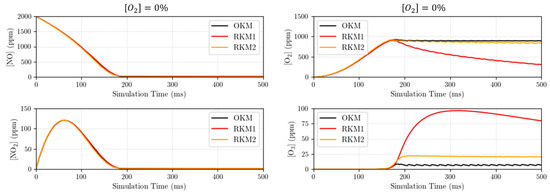
Figure 9.
Performance of the reduced mechanisms: transient variations in the species of interest (SOI) calculated with RKM1 (red) and RKM2 (orange) compared to OKM (black); time variations obtained with a gas mixture where .
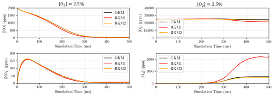
Figure 10.
Performance of the reduced mechanisms: transient time variations in the species of interest (SOI) calculated with RKM1 (red) and RKM2 (orange) compared to OKM (black; time variations obtained with a gas mixture where .
All the curves shown below use the same following color code: the OKM is displayed in black, RKM1 in red, and RKM2 in orange. If displayed, experimental measures are blue.
3.3. Robustness of Reduced Kinetic Mechanisms (RKM1 and RKM2) Concerning deNOX Process Performance
In the analysis displayed in this section, concentration varies over a wide range, from 400 ppm to 4000 ppm (step 400 ppm). The aim is to evaluate the ability of RKM1 and RKM2 to correctly translate the reduction in NOx, even when their input concentration is far from the condition selected to build reduced kinetic mechanisms (second step of the reduction process, detailed in Section 2.3.2. The operating conditions are given in Table 4).
To build the abaci,
- The temperature is kept at 450 K (uniform temperature distribution assumed in the reactor);
- The electrical power injection is the same for all simulations at 20 W, with the pattern described in Table 4;
- Different concentrations of , which is known to be an effective quencher and significantly disturbs NTP processes, are considered.
The three graphs below present the deNOx efficiency, with varied input concentrations. Experimental measurements are compared with the results provided by the three kinetic mechanisms.
3.4. Robustness of Reduced Kinetic Mechanisms (RKM1 and RKM2) with Respect to Experimental Conditions
The simulations performed in the previous sub-sections are associated with a specific operating point for the deNOx process. To check the robustness of the reduced mechanisms and their ability to provide reliable results under conditions different from the ones selected to build them, a systematic comparison is achieved: we consider the results obtained with the original kinetic mechanism (OKM) and with the reduced kinetic mechanisms RKM1 and RKM2 in various situations that are different from the one selected to build the RKMs:
3.4.1. Robustness with Respect to
Concentration
In this section, concentration varies in a wide range, from 0% to 20% (usual proportion in ambient air), with 0.5% steps below 3% and 1% after. The objective of the proposed analysis is to evaluate the robustness of the RKM1 and RKM2 mechanisms in situations that are vastly different from those used in establishing them (Table 4 describes this reference operating point).
To build the abaci in Figure 11,
- The temperature is kept at 450 K (uniform temperature distribution assumed in the reactor);
- The electrical power injection is the same for all simulations at 20 W, with the pattern described in Table 4;
- concentration is considered.

Figure 11.
Compared performances of the three mechanisms: deNOx process efficiency (%) vs. input concentration (ppm), calculated with RKM1, RKM2, and OKM and compared to experimental measurements. Three different concentrations are considered, 0% (top), 1% (middle), and 2.5% (bottom).
Figure 11.
Compared performances of the three mechanisms: deNOx process efficiency (%) vs. input concentration (ppm), calculated with RKM1, RKM2, and OKM and compared to experimental measurements. Three different concentrations are considered, 0% (top), 1% (middle), and 2.5% (bottom).

Below, in Figure 12, the graph on the left presents the performance of the deNOx process with respect to the concentration variation, estimated with the OKM, RKM1, and RKM2.
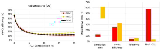
Figure 12.
Robustness of RKM1 and RKM2—figures of merit of the reduced kinetic mechanisms (with respect to the OKM) for large changes in concentration.
The graph on the right summarizes the simulation performance, displayed according to the following four criteria:
- Simulation time;
- deNOx efficiency (already displayed differently in the left graph);
- selectivity = , giving the percentage of injected transformed into ;
- concentration in the outlet gas mixture (after the residence time).
The bars represent the relative error estimated under each operating condition considered between the OKM and the RKM1 or RKM2 (the red bars correspond to the RKM1 and the orange bars to the RKM2): the bars extend between the minimum relative error and the maximum relative error and are centered on the average value of the relative error (calculated over all the operating conditions). The ideal match would be when this average value is close to 0%, with a very small bar amplitude (in the case of Figure 12, this is the case for “selectivity”).
The errors are considered in absolute value; hence, the average error given for the “simulation time” criterion is the reduction ratio obtained with RKM1 and RKM2 compared to OKM.
3.4.2. Robustness with Respect to Gas Temperature
In this section, temperature, which is known to significantly impact the deNOx process [10,26,36], varies across a wide range, from 300 K to 600 K with 50 K steps. The objective of the proposed analysis is to evaluate the robustness of the RKM1 and RKM2 mechanisms in situations where the temperature is vastly different from the one used to establish these reduced kinetic mechanisms (450 K, as mentioned in Table 4).
- The electrical power injection is the same for all simulations at 20 W, with the pattern described in Table 4;
- concentration is considered;
The graphs on the left present deNOx process performance with respect to the temperature variation, estimated with the OKM, RKM1, and RKM2.
As in the previous section, the graph on the right summarizes the simulation performance, displayed according to the following four criteria:
- Simulation time;
- deNOx efficiency (already displayed differently in the left graph);
- selectivity;
- concentration in the outlet gas mixture (after the residence time).
The bars represent the relative error estimated under each operating condition considered between the OKM and the RKM1 or RKM2 (the red bars correspond to the RKM1 and the orange bars to the RKM2): the bars extend between the minimum relative error and the maximum relative error and are centered on the average value of the relative error (calculated over all the operating conditions). The ideal match would be when this average value is close to 0%, with a very small bar amplitude (in the case of Figure 13, this is the case for “deNOx efficiency”).

Figure 13.
Robustness of RKM1 and RKM2—figures of merit of the reduced kinetic mechanisms (with respect to the original OKM) for large temperature changes; gas mixture without .
Figure 13.
Robustness of RKM1 and RKM2—figures of merit of the reduced kinetic mechanisms (with respect to the original OKM) for large temperature changes; gas mixture without .


Figure 14.
Robustness of RKM1 and RKM2—figures of merit of the reduced kinetic mechanisms (with respect to the original OKM) for large temperature changes; gas mixture .
Figure 14.
Robustness of RKM1 and RKM2—figures of merit of the reduced kinetic mechanisms (with respect to the original OKM) for large temperature changes; gas mixture .

4. Discussion
In this section, we reflect on the different results presented in the previous sections. These are grouped into different topics.
4.1. Accelerated Simulations to Facilitate the Design of Experimental and Industrial Configurations
The plots in Figure 4 and Figure 5 present a time response for the SOI computed with ZdPlaskin integrating the full original kinetic mechanism for different O2 concentrations: in the case where the input mixture contains , the selected residence time of 180 ms proves to be too short for complete NOx removal. It is therefore necessary to review the reactor design and operating conditions (power injection and input mass flow rate). Controlling the residence time is a fairly complex problem [10,30], as it depends on the gas temperature, which controls the speed of the gas mixture in the reactor. The temperature actually varies along the path [10] in the reactor, although in this paper, we have assumed a uniform temperature. Diagrams, such as those shown in Figure 6 and Figure 11, are also powerful tools for setting up experiments. The test bench presented in Section 2.1 is dedicated to this type of study. Given the information provided by ZdPlaskin, the advantages of simulations in accelerating the design of the experiment should be obvious.
4.2. Accuracy of Reduced Kinetic Mechanisms (RKM1, RKM2)
As can be seen in Figure 9 and Figure 10, in accordance with the difference in the input gas mixtures ( for Figure 9 and for Figure 10), the responses are different but show very good agreement between the three kinetic mechanisms (OKM, RKM1, RKM2) for the time evolutions of and .
Unsurprisingly, RKM1, which does not include and in its SOI, presents a noticeable difference to the OKM in its responses concerning these two species.
RKM2 appears almost perfect for the four species, with or without in the gas mixture. Even the difference shown in Figure 9 () for and must be put into perspective given the very low concentrations obtained; the values obtained can be considered to be within the range of the solver’s numerical integration errors.
Somehow, the errors in the results provided by RKM1 (mainly for and ) should be considered as the “price for speed-up” (let us remember the simulation times for the same 180 ms residence time—OKM: 500 s, RKM1: 82 s, RKM2: 213 s).
Figure 11 presents abaci with a wide range of concentrations in the input gas mixture (three different input concentrations are considered); the analysis focuses on the results concerning the NOx ( and ) obtained at the output of the reactor. The results provided by the OKM are used as references, together with experimental measurements. Figure 11 shows the results at the output of the generator from the three models after : assuming a uniform identical temperature distribution within the gas (450 K), the deNOx process efficiency (reduction in and concentrations) highlights reliable and similar trends provided by the three models. It confirms, for a wide range of concentrations, the result obtained in Figure 9 and Figure 10. One can notice that the results displayed for are almost perfectly superimposed. The explanation for such a performance is that the reduced models (RKM1 and RKM2) have been trained with OKM simulation results obtained with and .
It is again important to stress the strong decrease in the simulation costs through the reduced models shown in Table 2: considering the number of simulation runs necessary to build abaci such as those displayed at Figure 11, as well as figures of merit in Section 3.4, such an improvement is really valuable.
4.3. Robustness of Reduced Kinetic Mechanisms
Figure 11, Figure 12, Figure 13 and Figure 14 summarize the performance of the reduced kinetic mechanisms (RKM1 and RKM2) through a comparison with the results provided by the OKM. Although RKM1 and RKM2, devoted to two different sets of species of interest (SOI), were created using a specific operating condition (summarized in Table 4), their accuracy has been checked versus large variations:
- In the concentration in the input gas mixture; see Figure 11;
- In the concentration in the input gas mixture; see Figure 12;
A comparison of the reduced kinetic mechanisms with the OKM have been evaluated on
- A time simulation (with the same 180 ms residence time);
- deNOx treatment efficiency;
- deNOx treatment sensitivity;
- concentration in the outlet gas mixture.
The results of these analyses show a significant reduction in simulation time, which falls below 15% for RKM1 and below 50% for RKM2 (compared to the OKM). Only one case was observed where RKM2 required more time than the OKM (120% for a temperature of 300 K in the temperature scan).
Concerning the deNOx process, except for very high concentrations or for concentrations higher than 15% in the input gas, the error in deNOx efficiency is always less than 10% with both reduced mechanisms, even in the case of very large gas temperature variations.
Performance concerning deNOx selectivity versus variations do not show noticeable errors. On the contrary, if the temperature is varied, the errors are very small (below 3% for RKM1 and 8% for RKM2) as long as the temperature is below 500 K; but when this threshold is crossed, errors can rise over 300%.
The performance concerning the final concentration exhibits a behavior similar to the one observed for the selectivity, with very high errors over 500 K (up to 300% for RKM2 and even worse for RKM1, which does not include in its SOI), fair results below 400 K and almost perfect match between 400 K and 500 K.
One should remember that the reduced mechanisms were learnt at 450 K, which explains why the performance is the best in the 400K – 500K temperature range. This could possibly suggest improvements in the second step used for building the reduced kinetic mechanisms—better results should be obtained considering different temperatures instead of a single one. In the current state, we believe that temperatures over 500 K should be studied with the complete OKM.
5. Conclusions
In summary, the following outlines the key results of our study:
- NTP chemical simulation, using dedicated tools such as ZdPlaskin, can make a valuable contribution to the design of experimental setups;
- Reduced kinetic mechanisms focused on a specific set of species of interest (SOI) are able to drastically reduce the simulation time and allow for an intensive use of simulations;
- The proposed method for selecting a subset of chemical species and reactions focused on SOI based on the original kinetic mechanism has proven to be effective and capable of establishing robust kinetic mechanisms, particularly with regard to changes in the proportions of the input gas mixture; when temperature changes are taken into account, the robustness of the reduced mechanisms decreases when the selected operating conditions deviate too far from the reference temperature.
Author Contributions
Conceptualization, H.P. and N.B.; methodology, A.C.V., N.B. and H.P.; software, A.C.V.; validation, N.B.; investigation, N.B. and H.P.; data curation, N.B., A.C.V. and H.P.; writing—original draft preparation, N.B., A.C.V. and H.P.; writing—review and editing, H.P.; visualization, N.B.; supervision, H.P.; project administration, H.P. All authors have read and agreed to the published version of the manuscript.
Funding
This research received no external funding.
Institutional Review Board Statement
Not applicable.
Informed Consent Statement
Not applicable.
Data Availability Statement
The original contributions presented in this study are included in the article.
Acknowledgments
The authors sincerely thank G. Hagelaar for discussions and advice concerning ZdPlaskin, E. Bru, who made the “deNOx” test bench possible, and Toulouse INP for the support of A. Cuellar’s mobility (ETI-2025 program).
Conflicts of Interest
The authors declare no conflicts of interest.
Abbreviations
The following abbreviations are used in this manuscript:
| DBD | Dielectric Barrier Discharge |
| NTP | Non-Thermal Plasma |
| SOI | Species of Interest |
| OKM | Original Kinetic Mechanism |
| IKM | Initial Kinetic Mechanism |
| RKM | Reduced Kinetic Mechanism |
References
- Talebizadeh, P.; Babaie, M.; Brown, R.; Rahimzadeh, H.; Ristovski, Z.; Arai, M. The role of non-thermal plasma technique in NOx treatment: A review. Renew. Sustain. Energy Rev. 2014, 40, 886–901. [Google Scholar] [CrossRef]
- Rueda, V. Reduction of Nitrogen Oxides in Diesel Exhaust Using Dielectric Barrier Discharges Driven by Current-Mode Power Supplies. Ph.D. Thesis, Institut National Polytechnique de Toulouse—INPT, Toulouse, France, Pontificia Universidad Javeriana, Bogotá, Colombia, 2022. Available online: https://theses.hal.science/tel-04248330v1 (accessed on 27 July 2025).
- Alves, L.; Holz, L.I.V.; Fernandes, C.; Ribeirinha, P.; Mendes, D.; Fagg, D.P.; Mendes, A. A comprehensive review of NOx and N2O mitigation from industrial streams. Renew. Sustain. Energy Rev. 2022, 155, 111916. [Google Scholar] [CrossRef]
- Wang, Z.; Kuang, H.; Zhang, J.; Chu, L.; Ji, Y. Nitrogen oxide removal by non-thermal plasma for marine diesel engines. RSC Adv. 2019, 9, 5402–5416. [Google Scholar] [CrossRef] [PubMed]
- McLarnon, C.; Penetrante, B. Effect of Gas Composition on the NOx Conversion Chemistry in a Plasma. SAE Tech. Pap. 1998, 107, 982433. [Google Scholar] [CrossRef]
- Vinh, T.Q.; Watanabe, S.; Furuhata, T.; Arai, M. Fundamental study of NOx removal from diesel exhaust gas by dielectric barrier discharge reactor. J. Mech. Sci. Technol. 2012, 26, 1921–1928. [Google Scholar] [CrossRef]
- Anaghizi, S.J.; Talebizadeh, P.; Rahimzadeh, H.; Ghomi, H. The Configuration Effects of Electrode on the Performance of Dielectric Barrier Discharge Reactor for NOx Removal. IEEE Trans. Plasma Sci. 2015, 43, 1944–1953. [Google Scholar] [CrossRef]
- Kogelschatz, U. Dielectric-barrier discharges: Their History, Discharge Physics, and Industrial Applications. Plasma Chem. Plasma Process. 2003, 23, 1–46. [Google Scholar] [CrossRef]
- Wang, T.; Sun, B.M.; Xiao, H.P.; Zeng, J.Y.; Duan, E.P.; Xin, J.; Li, C. Effect of Reactor Structure in DBD for Nonthermal Plasma Processing of NO in N2 at Ambient Temperature. Plasma Chem. Plasma Process 2012, 32, 1189–1201. [Google Scholar] [CrossRef]
- Bente, N. Étude Système d’un Dispositif de Décharges à Barrières Diélectriques Dédié à la Réduction des Oxydes d’azote. Ph.D. Thesis, Institut National Polytechnique de Toulouse—INPT, Toulouse, France, 2025. Available online: https://theses.hal.science/tel-05185152v1 (accessed on 27 July 2025).
- Pancheshnyi, S.; Eismann, B.; Hagelaar, G.J.M.; Pitchford, L.C. Computer Code ZdPlaskin; University of Toulouse, LAPLACE, CNRS-UPS-INP: Toulouse, France, 2008; Available online: https://www.ZdPlaskin.laplace.univ-tlse.fr (accessed on 27 July 2025).
- Hagelaar, G.J.M.; Pitchford, L.C. Solving the Boltzmann equation to obtain electron transport coefficients and rate coefficients for fluid models. Plasma Sources Sci. Technol. 2005, 14, 722–733. [Google Scholar] [CrossRef]
- Pitchford, L.C.; Alves, L.L.; Bartschat, K.; Biagi, S.F.; Bordage, M.-C.; Bray, I.; Brion, C.E.; Brunger, M.J.; Campbell, L.; Chachereau, A.; et al. LXCat: An Open-Access, Web-Based Platform for Data Needed for Modeling Low Temperature Plasmas. Plasma Process. Polym. 2017, 14, 1600098. [Google Scholar] [CrossRef]
- Pancheshnyi, S.; Biagi, S.; Bordage, M.; Hagelaar, G.; Morgan, L.; Phelps, A.; Pitchford, L. The LXCat project: Electron scattering cross sections and swarm parameters for low temperature plasma modeling. Chem. Phys. 2012, 398, 148–153. [Google Scholar] [CrossRef]
- Carbone, E.; Graef, W.; Hagelaar, G.; Boer, D.; Hopkins, M.M.; Stephens, J.C.; Yee, B.T.; Pancheshnyi, S.; van Dijk, J.; Pitchford, L. Data Needs for Modeling Low-Temperature Non-Equilibrium Plasmas: The LXCat Project, History, Perspectives and a Tutorial. Atoms 2021, 9, 16. [Google Scholar] [CrossRef]
- Koelman, P.; Heijkers, S.; Mousavi, S.T.; Graef, W.; Mihailova, D.; Kozak, T.; Bogaerts, A.; van Dijk, J. A Comprehensive Chemical Model for the Splitting of CO2 in Non-Equilibrium Plasmas. Plasma Process. Polym. 2017, 14, 1600155. [Google Scholar] [CrossRef]
- Shao, X.; Lacoste, D.A.; Im, H.G. ChemPlasKin: A general-purpose program for unified gas and plasma kinetics simulations. Appl. Energy Combust. Sci. 2024, 19, 100280. [Google Scholar] [CrossRef]
- Tatar, M.; Vashisth, V.; Iqbal, M.; Butterworth, T.; van Rooij, G.; Andersson, R. Analysis of a plasma reactor performance for direct nitrogen fixation by use of three-dimensional simulations and experiments. Chem. Eng. J. 2024, 497, 154756. [Google Scholar] [CrossRef]
- Malé, Q.; Barléon, N.; Shcherbanev, S.; Dharmaputra, B.; Noiray, N. Numerical study of nitrogen oxides chemistry during plasma assisted combustion in a sequential combustor. Combust. Flame 2024, 260, 113206. [Google Scholar] [CrossRef]
- Rueda, V.; Wiesner, A.; Diez, R.; Piquet, H. Power Estimation of a Current Supplied DBD Considering the Transformer Parasitic Elements. IEEE Trans. Ind. Appl. 2019, 55, 6567–6575. [Google Scholar] [CrossRef]
- Florez, D.; Schitz, D.; Piquet, H.; Diez, R. Efficiency of an Exciplex DBD Lamp Excited Under Different Methods. IEEE Trans. Plasma Sci. 2018, 46, 140–147. [Google Scholar] [CrossRef]
- Manley, T.C. The Electric Characteristics of the Ozonator Discharge. Trans. Electrochem. Soc. 1943, 84, 83. [Google Scholar] [CrossRef]
- Díez, R.; Salanne, J.-P.; Piquet, H.; Bhosle, S.; Zissis, G. Predictive model of a DBD lamp for power supply design and method for the automatic identification of its parameters. Eur. Phys. J. Appl. Phys. 2007, 37, 307–313. [Google Scholar] [CrossRef]
- Penetrante, B.M.; Hsiao, M.C.; Merritt, B.T.; Vogtlin, G.E.; Wallman, P.H.; Neiger, M.; Wolf, O.; Hammer, T.; Broer, S. Pulsed corona and dielectric-barrier discharge processing of NO in N2. Appl. Phys. Lett. 1996, 68, 3719–3721. [Google Scholar] [CrossRef]
- Clyne, M.A.A.; McDermid, I.S. Mass spectrometric determinations of the rates of elementary reactions of NO and of NO2 with ground state N4S atoms. J. Chem. Soc. Faraday Trans. 1975, 71, 2189–2202. [Google Scholar] [CrossRef]
- Zhu, A.-M.; Sun, Q.; Niu, J.-H.; Xu, Y.; Song, Z.-M. Conversion of NO in NO/N2, NO/O2/N2, NO/C2H4/N2 and NO/C2H4/O2/N2 Systems by Dielectric Barrier Discharge Plasmas. Plasma Chem. Plasma Process 2005, 25, 371–386. [Google Scholar] [CrossRef]
- Tsang, W.; Herron, J.T. Chemical Kinetic Data Base for Propellant Combustion I. Reactions Involving NO, NO2, HNO, HNO2, HCN and N2O. J. Phys. Chem. Ref. Data 1991, 20, 609–663. [Google Scholar] [CrossRef]
- Atkinson, R.; Baulch, D.L.; Cox, R.A.; Hampson, R.F.; Kerr, J.A., Jr.; Troe, J. Evaluated Kinetic and Photochemical Data for Atmospheric Chemistry: Supplement IV. UPAC Subcommittee on Gas Kinetic Data Evaluation for Atmospheric Chemistry. J. Phys. Chem. Ref. Data 1992, 21, 1125. [Google Scholar] [CrossRef]
- Bente, N.; Piquet, H.; Merbahi, N.; Bru, E. Thermal modelling of an atmospheric pressure cylindrical DBD reactor for NOx removal. In Proceedings of the Europhysics Conference on Atomic and Molecular Physics of Ionized Gases (ESCAMPIG XXVI), Brno, Czech Republic, 9–13 July 2024; Available online: https://hal.science/hal-04639116v1 (accessed on 27 July 2025).
- Talebizadeh, P.; Rahimzadeh, H.; Babaie, M.; Anaghizi, S.J.; Ghomi, H.; Ahmadi, G.; Brown, R. Evaluation of Residence Time on Nitrogen Oxides Removal in Non-Thermal Plasma Reactor. PLoS ONE 2015, 10, e0140897. [Google Scholar] [CrossRef] [PubMed]
- Capitelli, M.; Ferreira, C.M.; Gordiets, B.F.; Osipov, A.I. Plasma Kinetics in Atmospheric Gases; Springer: Berlin/Heidelberg, Germany, 2000; pp. 229–250. [Google Scholar]
- Flitti, A.; Pancheshnyi, S. Gas heating in fast pulsed discharges in N2–O2 mixtures. Eur. Phys. J. Appl. Phys. 2009, 45, 21001. [Google Scholar] [CrossRef]
- Phelps, A.V. Cross sections and swarm coefficients for nitrogen ions and neutrals in N2 and argon ions and neutrals in Ar for energies from 0.1 eV to 10 keV. J. Phys. Chem. Ref. Data 1991, 20, 557–573. [Google Scholar] [CrossRef]
- Türtscher, P.L.; Reiher, M. Pathfinder—Navigating and Analyzing Chemical Reaction Networks with an Efficient Graph-Based Approach. J. Chem. Inf. Model. 2022, 63, 147–160. [Google Scholar] [CrossRef] [PubMed]
- Markosyan, A.H.; Luque, A.; Gordillo-Vázquez, F.J.; Ebert, U. PumpKin: A tool to find principal pathways in plasma chemical models. Comput. Phys. Commun. 2014, 185, 2697–2702. [Google Scholar] [CrossRef]
- Wang, T.; Sun, B. Effect of temperature and relative humidity on NOX removal by dielectric barrier discharge with acetylene. Fuel Process. Technol. 2016, 144, 109–114. [Google Scholar] [CrossRef]


Disclaimer/Publisher’s Note: The statements, opinions and data contained in all publications are solely those of the individual author(s) and contributor(s) and not of MDPI and/or the editor(s). MDPI and/or the editor(s) disclaim responsibility for any injury to people or property resulting from any ideas, methods, instructions or products referred to in the content. |
© 2025 by the authors. Licensee MDPI, Basel, Switzerland. This article is an open access article distributed under the terms and conditions of the Creative Commons Attribution (CC BY) license (https://creativecommons.org/licenses/by/4.0/).