On the Effect of Electron Streaming and Existence of Quasi-Solitary Mode in a Strongly Coupled Quantum Dusty Plasma—Far and Near Critical Nonlinearity

Abstract

A strongly coupled quantum dusty plasma consisting of electrons and dust with the ions in the background is considered when there is streaming of electrons. It is observed that the streaming gives rise to both the slow and fast modes of propagation. The nonlinear mode is then analyzed by the reductive perturbation approach, resulting in the KdV-equation. In the critical situation where non-linearity vanishes, the modified scaling results in the MKdV equation. It is observed that both the KdV and MKdV equations possess quasi-solitary wave solution, which not only has the character of a soliton but also has a periodic nature. Such types of solitons are nowadays called nanopteron solitons and are expressed in terms of cnoidal-type elliptic functions.

1. Introduction

The interest in study of plasmas containing dust particles are growing day by day, because of the importance of such plasmas in the study of the space environment, such as asteroid zones, planetary rings, cometary tails as well as lower ionosphere of earth. The dust-in-plasma or the dusty plasma contain dust grains, which has a dimension of the order of micrometer to sub-micrometer [1,2,3].

Quantum aspects of plasma gained importance in recent times due to its application in plasma echoes [4] and micro-electronic devices [5]. Initially the subject was formulated and studied by Haas [6] and his collaborators [7]. It has applications in Fermi gas [8], quantum Penrose diagrams and quantum plasma instabilities [9]. Moreover, the quantum hydrodynamic model deals only with the macroscopic variables, namely the density and velocity stress tensors, etc., and also includes the so called Bohm potential [10]. On the other hand a different approach of quantum plasma is that of Wigner-Poisson equation, which is actually a kinetic model [11]. However, it is less effective in numerical simulations compared to that of the Q.H.D. (Quantum Hydrodynamic Model).

Actually, the field of quantum plasma physics has a long and diverse tradition and is garnering increasing interest that is motivated by its potential applications in modern technology. The quantum degeneracy effects start playing a significant role when the de Broglie thermal wavelength $\lambda =\frac{\hslash }{\sqrt{2\pi m_e{k}_{B}T}}$ for electrons is similar to or larger than the average interelectron distance ‘$n_e^{1/3}$’. Moreover, one can show that when the temperature approaches the electron Fermi temperature $T_{Fe}$, the equilibrium distribution function changes from the Maxwell–Boltzmann $\propto exp(-E/k_{B}T)$ to the Fermi–Dirac one.

Another important domain of present day plasma physics is the study of dusty plasma [12], and thus many analyses have been performed on quantum dusty plasma [13,14]. The emergence of the dust acoustic wave (D.A.W) is an important aspect of such analysis [15]. Dust Acoustic Waves (DAW) have been discussed in connection with various structures that have been observed in Saturn rings, such as spokes, braids and clumps [16]. The study of quantum plasma has been extensively performed by Haas [17], Shukla [18] and many others. However, in the domain of dusty plasma, the important phenomenon is of strong coupling of dust particles [19]. The corresponding investigation has been performed at least in two main formulations: one is to use the visco-elastic model [20] and the other by using effective electrostatic pressure [21]. It was Ikezi [22] who predicted that a dusty plasma can enter the strong coupling regime due to high charge and low temperature of the dust that makes the coupling co-efficient $\Gamma \gg 1$, and the coupling co-efficient $\mathsf{\Gamma }=\frac{e^2{Z}_d^2}{4\pi {\epsilon }_0{k}_B{T}_d{a}_d}$ is the ratio between the Coulomb potential energy and thermal energy used to measure the relative importance of these electrostatic forces on the dust grain. Here ‘$T_d$’, ‘$Z_d$’ and ‘$a_d=n_d^{1/3}$’ are the temperature, charge number and mean inter-particle distance of the dust, respectively. The equation of the state of strongly coupled plasma was formulated by Cousens et al. [23] and written as $P^{\ast }=n_d{k}_B{T}^{\ast }$, the effective electrostatic pressure. ‘$T^{\ast }$’ is the effective electrostatic temperature defined as $k_B{T}^{\ast }=\frac{N_{nn}{e}^2{Z}_d^2}{12\pi {\epsilon }_0}\sqrt[3]{n_d}(1+\mathcal{K})exp(-\mathcal{K})$ where ‘$N_{nn}$’ is the number of nearest neighbors determined by the normalized inter-particle distance.

On the other-hand, quantum dusty plasma [22] is well known as the feature of high charge and low temperature of dust grains with high number density compared with that of classical plasma, which renders the existence of strongly coupled regimes appearing in quantum plasma possible.

In the first part, we analyzed the linear mode of propagation by starting with the normalized electron-dust-ion equation, where we have assumed that the electrons possess a streaming velocity. The immediate consequence is that we obtain a fast and slow mode of propagation in the dusty plasma. In the next section we applied the reductive perturbation scheme in order to deduce the KdV equation, and it is found that we have a new kind of nonlinear excitation, which is a soliton having a periodic tail. In the next part, we consider the critical case when the nonlinearity coefficient tends to zero and the usual modification of the reductive computation results in the MKdV situation. Such an equation is also observed to posses a cnoidal-type soliton.

2. Formulation

Let us consider a plasma where ‘$n_e$’ is the electron density, ‘$u_e$’ is the corresponding velocity and the same quantities for the dust particle are denoted as ‘$n_d$’, ‘$u_d$’. The mass of electron and dust are denoted as ‘$m_e$’, ‘$m_d$’ respectively. If these are in motion then there will be an electrostatic potential ‘$\varphi$’ and pressure ‘$P_d$’. The Quantum Hydrodynamic (QHD) equations are as follows:

$$\frac{\partial n_e}{\partial t}+\frac{\partial }{\partial x}\left(n_e{u}_e\right)=0$$

(1)

$$\frac{\partial u_e}{\partial t}+u_e\frac{\partial u_e}{\partial x}=\frac{{\hslash }^2}{2m_e^2}\frac{\partial }{\partial x}\left\{\frac{{\partial }^2/\partial x^2\left(\sqrt{n_e}\right)}{\sqrt{n_e}}\right\}+\frac{e}{m_e}\frac{\partial \varphi }{\partial x}$$

(2)

$$\frac{\partial n_d}{\partial t}+\frac{\partial }{\partial x}\left(n_d{u}_d\right)=0$$

(3)

$$\frac{\partial u_d}{\partial t}+u_d\frac{\partial u_d}{\partial x}=\frac{{\hslash }^2}{2m_d^2}\frac{\partial }{\partial x}\left\{\frac{{\partial }^2/\partial x^2\left(\sqrt{n_d}\right)}{\sqrt{n_d}}\right\}-\frac{e}{m_d}\frac{\partial \varphi }{\partial x}-\frac{\partial P_d}{\partial x}$$

(4)

$$\frac{{\partial }^2\varphi }{\partial x^2}=\frac{e}{{\epsilon }_0}(n_e+n_d-n_0)$$

(5)

‘$\varphi$’ is the electrostatic potential here. Moreover, we consider the ions to be immobile and to have a distribution of the following form.

$$n_0=n_{i0}exp(-\frac{e\varphi }{k_B{T}_i})$$

(6)

The normalized set of equation governing the dusty plasma can be written as follows:

$$\frac{\partial n_e}{\partial t}+\frac{\partial }{\partial x}\left(n_e{u}_e\right)=0$$

(7)

$$\frac{\partial u_e}{\partial t}+u_e\frac{\partial u_e}{\partial x}=H^2{\alpha }_1\frac{\partial }{\partial x}\left\{\frac{{\partial }^2/\partial x^2\left(\sqrt{n_e}\right)}{\sqrt{n_e}}\right\}+\frac{{\alpha }_1}{Z_d}\frac{\partial \varphi }{\partial x}$$

(8)

$$\frac{\partial n_d}{\partial t}+\frac{\partial }{\partial x}\left(n_d{u}_d\right)=0$$

(9)

$$\frac{\partial u_d}{\partial t}+u_d\frac{\partial u_d}{\partial x}=H^2{\alpha }_1\frac{\partial }{\partial x}\left\{\frac{{\partial }^2/\partial x^2\left(\sqrt{n_d}\right)}{\sqrt{n_d}}\right\}-\frac{\partial \varphi }{\partial x}-\frac{1}{Z_d}\frac{\partial \left(n_{d}d\right)}{\partial x}$$

(10)

$$\frac{{\partial }^2\varphi }{\partial x^2}={\mu }_1{n}_e+n_d-\beta exp(-S\varphi )$$

(11)

where the normalized distribution for the background ions is as follows

$$n_0=\beta exp(-S\varphi )$$

(12)

with ${\mu }_1=\frac{n_{e0}}{Z_d{n}_{d0}}$, $\beta =\frac{n_{i0}}{Z_d{n}_{d0}}$ and $S=\frac{T_0}{T_i}$ where ‘$n_{i0}$’ and ‘$n_{e0}$’ are, respectively, the ion-electron equilibrium densities, and ‘$T_i$’ and ‘$T_e$’ are their temperatures with $T_0=\frac{Z_d^2{n}_{d0}{T}_i{T}_e}{n_{i0}{T}_e+n_{e0}{T}_i}$, where we have used all the scaled variables. Here ‘$u_e$’ and ‘$n_e$’ are the velocity and density of electrons, ‘$u_d$’, ‘$n_d$’ are those of the dust grains and ‘$\varphi$’ is the electrostatic potential. The strong interaction between the dust grains are expressed as a force given by the potential.

The normalized variables are defined as $t\to {\omega }_{pd}t$; $x\to x/{\lambda }_D$; $u_d\to u_d/C_d$; $u_e\to u_e/C_d$; $n_d\to n_d/n_{d0}$; $n_e\to n_e/n_{e0}$; and $\varphi \to \varphi /\left(\frac{k_B{T}_0}{e}\right)$, where ${\omega }_{pd}=\sqrt{\frac{Z_d^2{e}^2{n}_{d0}}{{ϵ}_0{m}_d}}$; $\lambda =\sqrt{\frac{{ϵ}_0{k}_B{T}_0}{Z_d^2{n}_{d0}{e}^2}}$; and $C_d=\sqrt{\frac{Z_d{k}_B{T}_0}{m_d}}$.

3. Linear Propagation and Streaming

In order to analyse the linear propagation mode, we set the following:

$$\left.\begin{array}{c}\hfill n_e=1+n_{e1}exp\left[i(kx-\omega t)\right]\\ \hfill u_e=u_{e0}+u_{e1}exp\left[i(kx-\omega t)\right]\\ \hfill n_d=1+n_{d1}exp\left[i(kx-\omega t)\right]\\ \hfill u_d=u_{d1}exp\left[i(kx-\omega t)\right]\\ \hfill \varphi ={\varphi }_{1}exp\left[i(kx-\omega t)\right]\\ \hfill d=d_0+ϵd_1\end{array}\right\}$$

(13)

where $d_1=d_{11}{n}_{d1}+d_{12}{\varphi }_1$ (from Reference [23]) provided that, at equilibrium, $Z_d{n}_{e0}+n_{d0}=Z_d{n}_{i0}$. Linearizing the set (7)–(12) results in the following.

$$n_{e1}=\frac{k}{\omega -k{u}_{e0}}{u}_{e1}$$

(14)

$$u_{e1}=\left\{\frac{k{Z}_d{\alpha }_1}{(\omega -k{u}_{e0})\left[1-\frac{H^2{k}^4}{2}\frac{{\alpha }_1}{{(\omega -k{u}_{e0})}^2}\right]}\right\}{\varphi }_1$$

(15)

$$n_{d1}=\frac{k}{\omega }{u}_{d1}$$

(16)

$$u_{d1}=-\frac{(d_{12}+1)(1/Z_d)(k/\omega )}{\left[1-\frac{H^2{k}^4}{2}+\frac{1}{Z_d}(d_0+d_{11})\frac{k^2}{{\omega }^2}\right]}{\varphi }_1$$

(17)

$$-k^2{\varphi }_1={\mu }_1{n}_{e1}+n_{d1}+\beta {\varphi }_1$$

(18)

These relations along with the equilibrium condition results in the following dispersion relation.

$$\begin{array}{c}\hfill \left(k^2+S\beta \right)+\frac{{\mu }_1{Z}_d{\alpha }_1{k}^2}{\left[{\left(\omega -k{u}_{e0}\right)}^2-\frac{H^2{k}^4{\alpha }_1}{2}\right]}-\frac{k^2(d_{12}+1)}{Z_d}\times \\ \hfill \frac{1}{\left[{\omega }^2-\frac{H^2{k}^4{\alpha }_1}{2}+\frac{(d_0+d_{11})k^2}{Z_d}\right]}=0\end{array}$$

(19)

Equation (19) can also be written as follows:

$${\omega }^4+a{\omega }^3+b{\omega }^2+c\omega +d=0$$

(20)

where $a=-\frac{2k{u}_{e0}}{(k^2+S\beta )}$; $b=(-{\mathsf{\Gamma }}_2{k}^4+{\mathsf{\Gamma }}_3{k}^2-{\mathsf{\Gamma }}_1{k}^4+k^2{u}_{e0}^2-{\mathsf{\Gamma }}_5{k}^2)$; $c=[(k^2+S\beta )(2k^5{u}_{e0}{\mathsf{\Gamma }}_2-2k{u}_{e0}{\mathsf{\Gamma }}_3{k}^2)-{\mathsf{\Gamma }}_5{k}^3{u}_{e0}]/(k^2+S\beta )$; $d=[(k^2+S\beta )(-k^6{u}_{e0}^2{\mathsf{\Gamma }}_2+{\mathsf{\Gamma }}_3{u}_{e0}^2{k}^4+{\mathsf{\Gamma }}_1{\mathsf{\Gamma }}_2{k}^8-{\mathsf{\Gamma }}_1{\mathsf{\Gamma }}_3{k}^6)-{\mathsf{\Gamma }}_4{k}^2({\mathsf{\Gamma }}_2{k}^4+{\mathsf{\Gamma }}_3{k}^2)-{\mathsf{\Gamma }}_5{k}^2(k^2{u}_{e0}^2-{\mathsf{\Gamma }}_1{k}^4)]/(k^2+S\beta )$.

We also have the following: ${\mathsf{\Gamma }}_1=\frac{H^2{k}^4{\alpha }_1}{2}$; ${\mathsf{\Gamma }}_2=\frac{H^2{k}^4{\alpha }_1}{2}$; ${\mathsf{\Gamma }}_3=\frac{d_0+d_{11}{k}^4}{Z_d}$; ${\mathsf{\Gamma }}_4={\mu }_1{Z}_d{\alpha }_1{k}^2$; $\frac{1}{Z_d}(d_{12}+1)k^2$.

The solution of the quartic Equation (20) is as follows:

$$\left.\begin{array}{c}\hfill {\omega }_{1,2}=-\frac{1}{2}\left(\frac{a}{2}+B\right) \pm \frac{1}{2}\sqrt{{\left(\frac{a}{2}+B\right)}^2-4(A+E)}\\ \hfill {\omega }_{3,4}=-\frac{1}{2}\left(\frac{a}{2}-B\right) \pm \frac{1}{2}\sqrt{{\left(\frac{a}{2}-B\right)}^2-4(A-E)}\end{array}\right\}$$

(21)

where the following is the case.

• $A=\frac{b}{3}+{\left(\frac{q}{2}\pm \frac{1}{2}\sqrt{q^2-\frac{4}{27}{p}^3}\right)}^{1/3}+{\left(\frac{q}{2}\mp \frac{1}{2}\sqrt{q^2-\frac{4}{27}{p}^3}\right)}^{1/3}$
• $p=3{\chi }^2-2\chi b+\theta$; $q={\chi }^3-b{\chi }^2+\theta \chi +\lambda$; $\chi =b/3$; $\theta =(1/4)(2ca-4d)$; $(1/4)(bd-a^{2}d-c^2)$; $B=\sqrt{\frac{a^2}{4}+A-b}$; $E=\sqrt{A^2-d}$

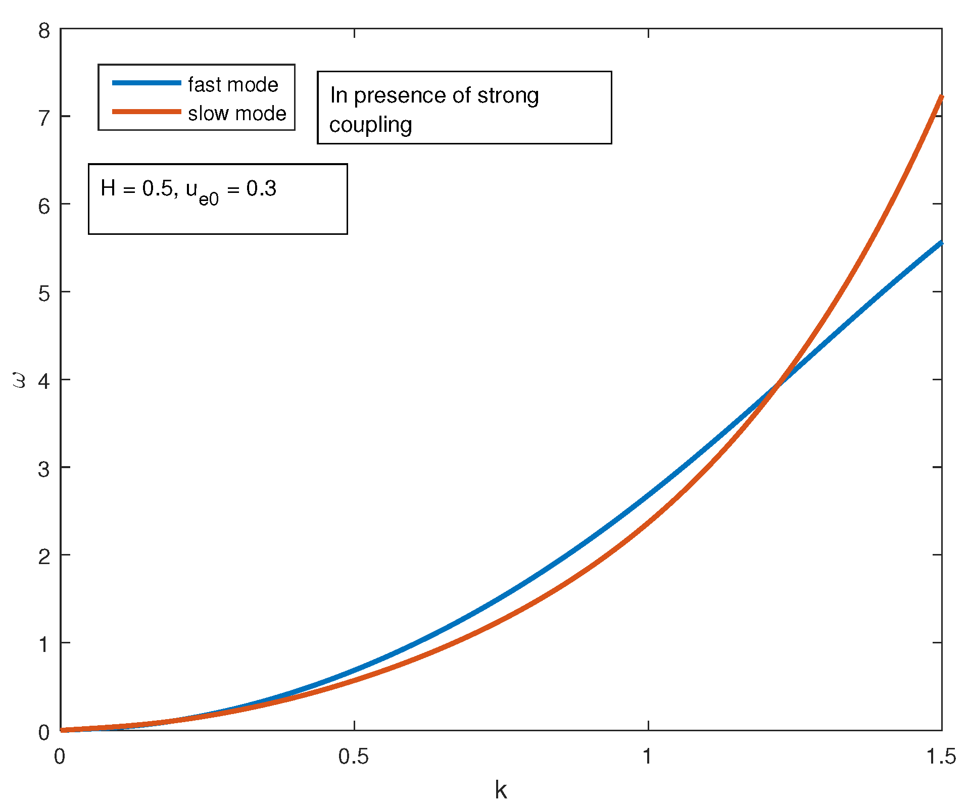
From the equation set (21), one can observe that ‘${\omega }_1$’ and ‘${\omega }_3$’ are physically admissible of the one that gives the slow mode and the other that gives the fast mode. In order to obtain an idea of the physical situation, we have graphically plotted the linear dispersion relation in Figure 1, Figure 2, Figure 3, Figure 4, Figure 5, Figure 6, Figure 7 and Figure 8. 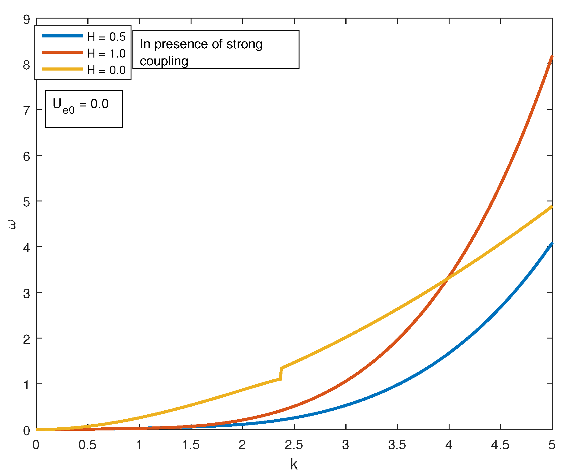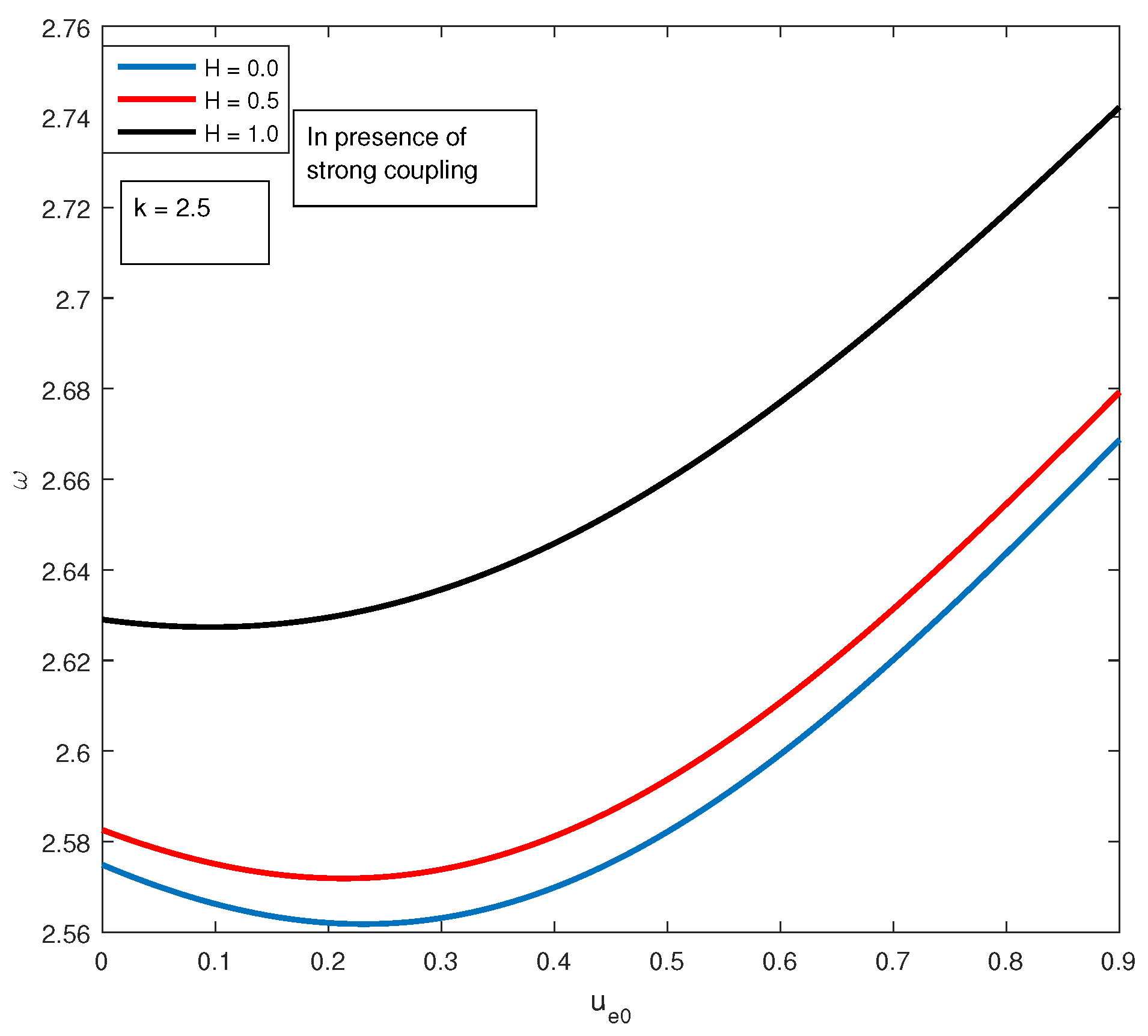In Figure 1 we show the case where there is no streaming or ‘$u_{e0}=0$’ and the effect of strong coupling is also absent, while in Figure 2 we have shown the situation where there is no streaming but the strong coupling effect is present and as a result the nature of variation of the dispersion relation changes. Moreover due to the presence of strong coupling the wave frequency also gets increased.

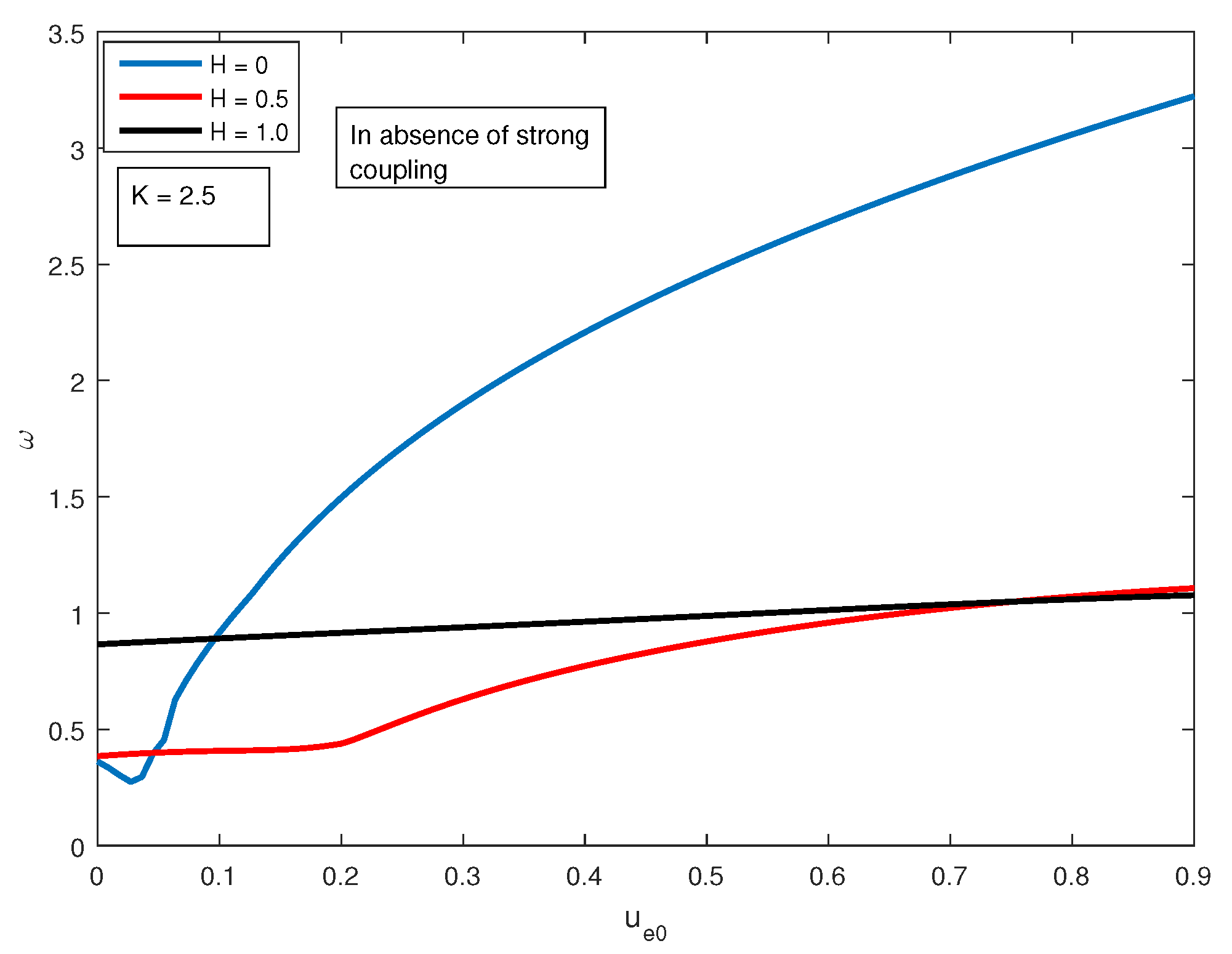
One should note that in both the Figure 1 and Figure 2, we observe that the quantum diffraction parameter ‘H’ has a very prominent effect. Next, in the Figure 3 and Figure 4, we have shown the variation of the wave frequency with the streaming velocity ‘$u_{e0}$’ both in the presence and absence of strong coupling effect.

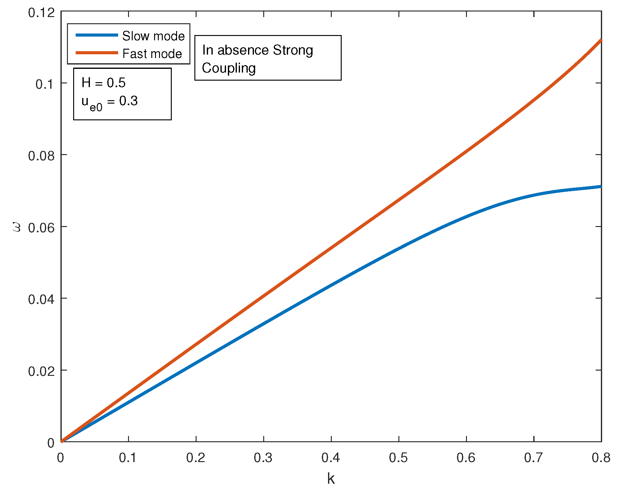
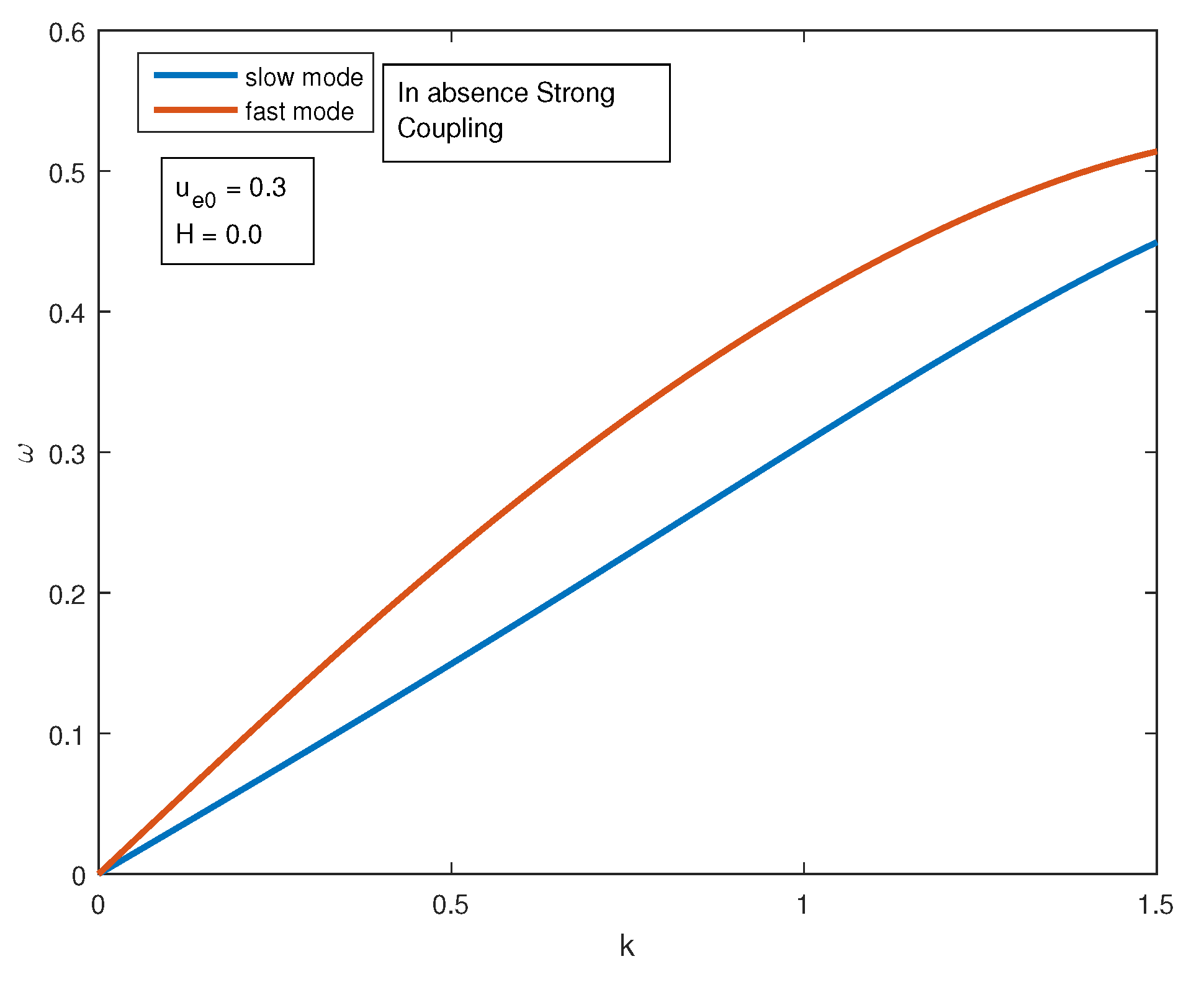
In the Figure 5, Figure 6, Figure 7 and Figure 8, we show how the electron streaming gives rise to two modes, namely ‘slow’ and ‘fast’, and how they vary with the diffraction parameter ‘H’, streaming velocity ‘$u_{e0}$’ and the effect of strong coupling.

4. Reductive Perturbation Approach and the Derivation of the Kdv Equation

In order to analyze the nonlinear propagating mode of the system, we adapt the reductive approach and set the following:

$$\left.\begin{array}{c}\hfill \xi ={ϵ}^{1/2}(x-\lambda t)\\ \hfill \tau ={ϵ}^{3/2}t\end{array}\right\}$$

(22)

along with

$$\left.\begin{array}{c}\hfill n_e=1+ϵn_{e1}+{ϵ}^2{n}_{e2}+{ϵ}^3{n}_{e3}+\cdots \\ \hfill u_e=u_{e0}+ϵu_{e1}+{ϵ}^2{u}_{e2}+{ϵ}^3{u}_{e3}+\cdots \\ \hfill n_d=1+ϵn_{d1}+{ϵ}^2{n}_{d2}+{ϵ}^3{n}_{d3}+\cdots \\ \hfill u_d=ϵu_{d1}+{ϵ}^2{u}_{d2}+{ϵ}^3{u}_{d3}+\cdots \\ \hfill \varphi =ϵ{\varphi }_1+{ϵ}^2{\varphi }_2+{ϵ}^3{\varphi }_3+\cdots \\ \hfill d=d_0+ϵd_1+{ϵ}^2{d}_2+{ϵ}^3{d}_3+\cdots \end{array}\right\}$$

(23)

whence in lowest order of $ϵ$ we obtain the following.

$$\left.\begin{array}{c}\hfill n_{e1}=\frac{u_{e1}}{(\lambda -u_{e0})}\\ \hfill n_{d1}=\frac{u_{e1}}{\lambda }\\ \hfill u_{e1}=-\frac{{\alpha }_3}{Z(\lambda -u_{e0})}{\varphi }_1\\ \hfill u_{d1}=-\frac{(d_{12}+1)Z}{Z{\lambda }^2-(d_0+d_{11})}{\varphi }_1\\ \hfill n_{d1}+{\mu }_1{n}_{e1}+S\beta {\varphi }_1=0\end{array}\right\}$$

(24)

This results in the dispersion relation for the long wavelength situation.

$$-\frac{{\alpha }_1{\mu }_1}{Z_d{(\lambda -u_{e0})}^2}+\frac{(d_{12}-1)}{\left[{\lambda }^2-(d_0+d_{11})\right]}+S\beta =0$$

(25)

In the next order of $ϵ$, that is, from the terms of ${ϵ}^{5/2}$, we obtain the following:

$$\frac{\partial n_{e1}}{\partial \tau }-\lambda \frac{\partial n_{e2}}{\partial \xi }+\frac{\partial u_{e2}}{\partial \xi }+\frac{\partial }{\partial \xi }\left(n_{e1}{u}_{e1}\right)+u_{e0}\frac{\partial n_{e2}}{\partial \xi }=0$$

(26)

$$\frac{\partial n_{d1}}{\partial \tau }-\lambda \frac{\partial n_{d2}}{\partial \xi }+\frac{\partial u_{d2}}{\partial \xi }+\frac{\partial }{\partial \xi }\left(n_{d1}{u}_{d1}\right)=0$$

(27)

$$\frac{\partial u_{e1}}{\partial \tau }-\lambda \frac{\partial u_{e2}}{\partial \xi }+u_{e0}\frac{\partial u_{e2}}{\partial \xi }+u_{e1}\frac{\partial u_{e1}}{\partial \xi }={\alpha }_1{H}^2\frac{{\partial }^3{n}_{e1}}{\partial {\xi }^3}+\frac{{\alpha }_3}{Z}\frac{\partial {\varphi }_2}{\partial \xi }$$

(28)

$$\begin{array}{c}\hfill \frac{\partial u_{d1}}{\partial \tau }-\lambda \frac{\partial u_{d2}}{\partial \xi }+u_{e1}\frac{\partial u_{e1}}{\partial \xi }={\alpha }_1{H}^2\frac{{\partial }^3{n}_{d1}}{\partial {\xi }^3}-\\ \hfill \frac{1}{Z}\frac{\partial }{\partial \xi }\left(d_0{n}_{d2}\right)-\frac{\partial {\varphi }_2}{\partial \xi }-\frac{1}{Z}\frac{\partial d_2}{\partial \xi }-\frac{1}{Z}\frac{\partial }{\partial \xi }\left(n_{d1}{d}_1\right)\end{array}$$

(29)

$$\frac{{\partial }^2{\varphi }_1}{\partial {\xi }^2}=n_{d2}+{\mu }_1{n}_{e2}-S\beta {\varphi }_2+\beta S^2{\varphi }_1^2$$

(30)

If we eliminate all higher order terms, we obtain the KdV equation:

$$\frac{\partial {\varphi }_1}{\partial \tau }+A\varphi \frac{\partial {\varphi }_1}{\partial \xi }+B\frac{{\partial }^3{\varphi }_1}{\partial {\xi }^3}=0$$

(31)

with $A=A_1/A_2$ and $B=B_1/A_2$, where ‘$A_1$’, ‘$A_2$’ and ‘$B_1$’ are given in Appendix A. The expression of ‘$d_2$’ in Equation (29) is given by $d_2=d_{21}{n}_2+d_{22}{\varphi }_2+d_{23}{n}_1^2+d_{24}{n}_1{\varphi }_1{d}_{25}{\varphi }_1^2$, where the constants $d_{21}$ and $d_{22}$, etc., are given as per Reference [23].

4.1. Soliton Cnoidal Wave Solution

It is well known that the KdV-equation wrote above always supports stationary wave solutions. However, recent studies have revealed a whole new class of solutions for the KdV problem. It may be mentioned that Boyd observed that one can numerically obtain a new class of solutions that does not follow the definition of soliton in the very strict sense, which is in the sense that it has a long tail that is a periodic waveform. Such novel kinds of patterns are named the ‘nanopteron’ solitons. These are a wide class known as the quasi-soliton. Later on, it was found that one can obtain the analytic form of such a solution by using the famous ‘tanh’-expansion method.

Let us set the following:

$${\varphi }_1=u_0+u_{1}tanh\left(w\right)+u_{2}tanh{\left(w\right)}^2$$

(32)

where, $u_0$, $u_1$, $u_2$ and w are functions of $(x,t)$ to be determined. By substituting Equation (36) in (35) and equating various powers of $tanh\left(w\right)$, a system of over-determined equations are obtained. It is really interesting to note that all these are consistent with one another. Finally, one obtains $u_2=-\frac{12B{w}_x^2}{A}$ and $u_1=\frac{12B{w}_{xx}}{A}$:

$$\frac{B}{A}\left(\frac{w_{xxx}}{w_x}-\frac{3w_{xx}^2}{2w_x^2}-2w_x^2\right)\frac{w_t}{A{w}_x}$$

along with the fact that $w(x,t)$ satisfies the following.

$$\frac{w_t}{w_x}+B\left(\frac{w_{xxx}}{w_x}-\frac{3w_{xx}^2}{2w_x^2}-2w_x^2\right)+\lambda =0$$

(33)

This $\lambda$ is a constant of integration. This last equation actually possesses a wide variety of solutions of which we only consider the following one:

$$w=\xi +c_1{tanh}^{-1}\left(c_{2}sn(\eta ,m)\right)$$

(34)

with the following.

$$\left.\begin{array}{c}\hfill \xi =\frac{x-V_{1}t}{W_1}\\ \hfill \eta =\frac{x-V_{2}t}{W_2}\end{array}\right\}$$

(35)

‘$sn$’ is the Jacobi-elliptic function with ellipticity ‘m’. It is interesting to note that ‘$V_1$’ and ‘$V_2$’ are the velocities of the soliton and the surrounding cnoidal wave. Thus, we can finally write the solution for ${\varphi }_1$:

$$\begin{array}{c}\hfill {\varphi }_1=\frac{3(V_1-V_2)}{2A{G}^2}\left[\frac{{(m^2-1+2G)}^2}{(m^2-1)}tanh{\left(w\right)}^2-\right.\\ \hfill \left.2\delta mS(m^2-1+2G)tanh\left(w\right)+(m^2-1)\right]-\\ \hfill \frac{(m^2+7)V_1-(3m^2+5)V_2}{2A(m^2-1)}\end{array}$$

(36)

with the following.

$$\left.\begin{array}{c}\hfill w=\frac{\xi -V_1\tau }{w_1}+c_1{tanh}^{-1}\left(c_{2}S(\eta ,m)\right)\\ \hfill G=1-m^2{S}^2+\delta mCD\\ \hfill \eta =\frac{\xi -V_2\tau }{w_2}\\ \hfill S=sn(\eta ,m);C=cn(\eta ,m);D=dn(\eta ,m)\\ \hfill W_1=\sqrt{\frac{8B(1-m^2)}{V_1-V_2}}\\ \hfill W_2=\sqrt{\frac{2B(1-m^2)}{V_1-V_2}}\\ \hfill c_1=\delta /2;c_2=m;{\delta }^2=1\end{array}\right\}$$

(37)

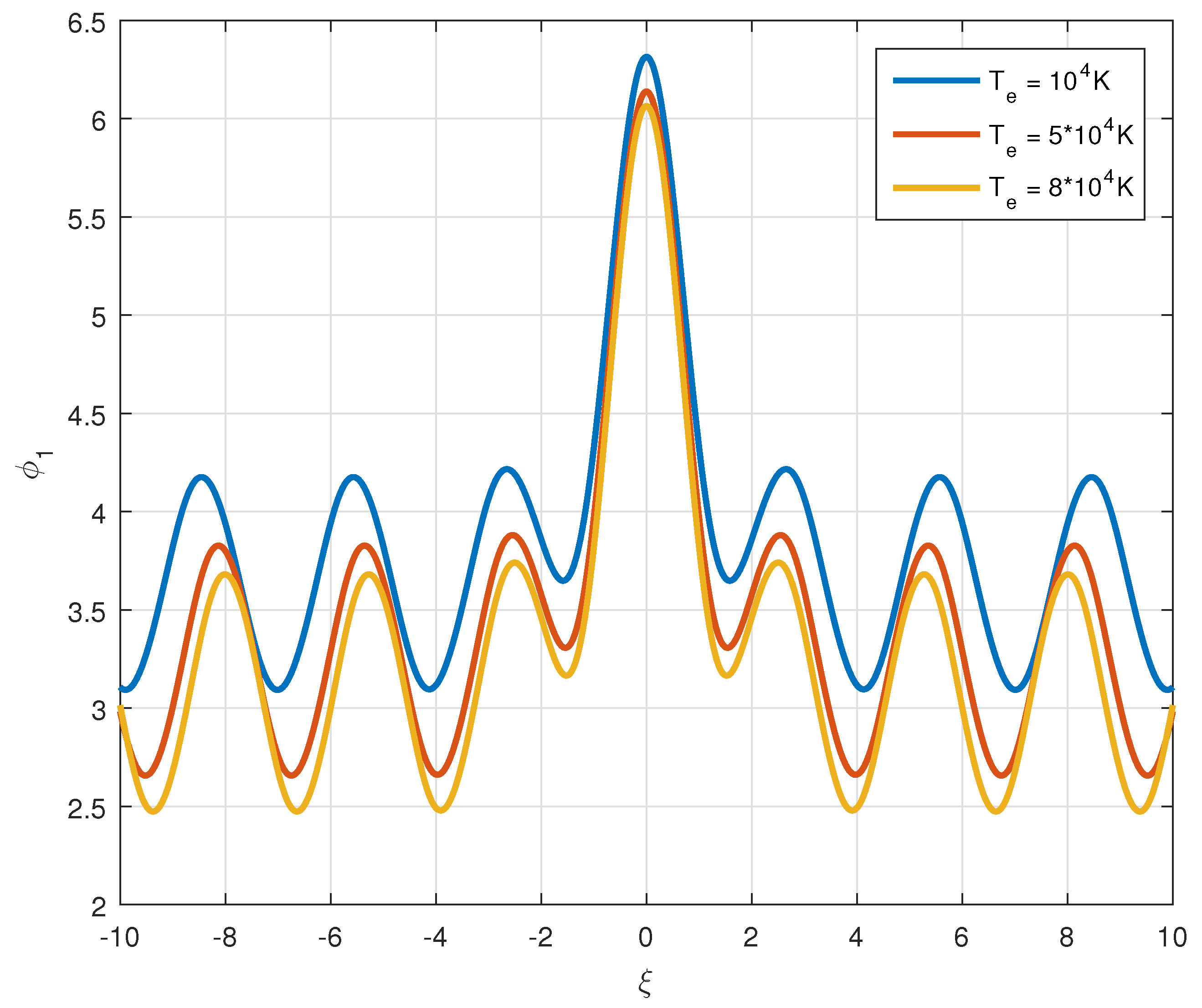
It is now interesting to observe that for $m_e=9.1\ast {10}^{-31}$ kg; $m_i=6.7\ast {10}^{-26}$ kg; $m_d=8\ast {10}^{-12}$ kg; $n_{e0}=4\ast {10}^{13}{\mathrm{m}}^{-3}$; $n_{i0}=7\ast {10}^{13}{\mathrm{m}}^{-3}$; $T_i=$ 11,600 kelvin; $T_e={10}^4$ kelvin; $T_e=5\ast {10}^4$ kelvin; $T_e=8\ast {10}^4$ kelvin; $Z=4.3\ast {10}^5$; $u_{e0}=1.5$; m = 0.04; $\delta =-1$; and $V_1=0.05$; $V_2=-0.05$, the form of ${\varphi }_1$ if plotted against $\xi$ turns out to be of the form given in Figure 9.

One may note that here we have a central solitary profile, but its tails are not approaching zero in either direction of $\xi$. Instead, we have purely sinusoidal behaviour such as $\xi \to \pm \infty$. We have shown how the form changes with the electron temperature $T_e$. On the other-hand, if one has $m=0$, then we obtain the purely solitary wave, as shown in the Figure 10.

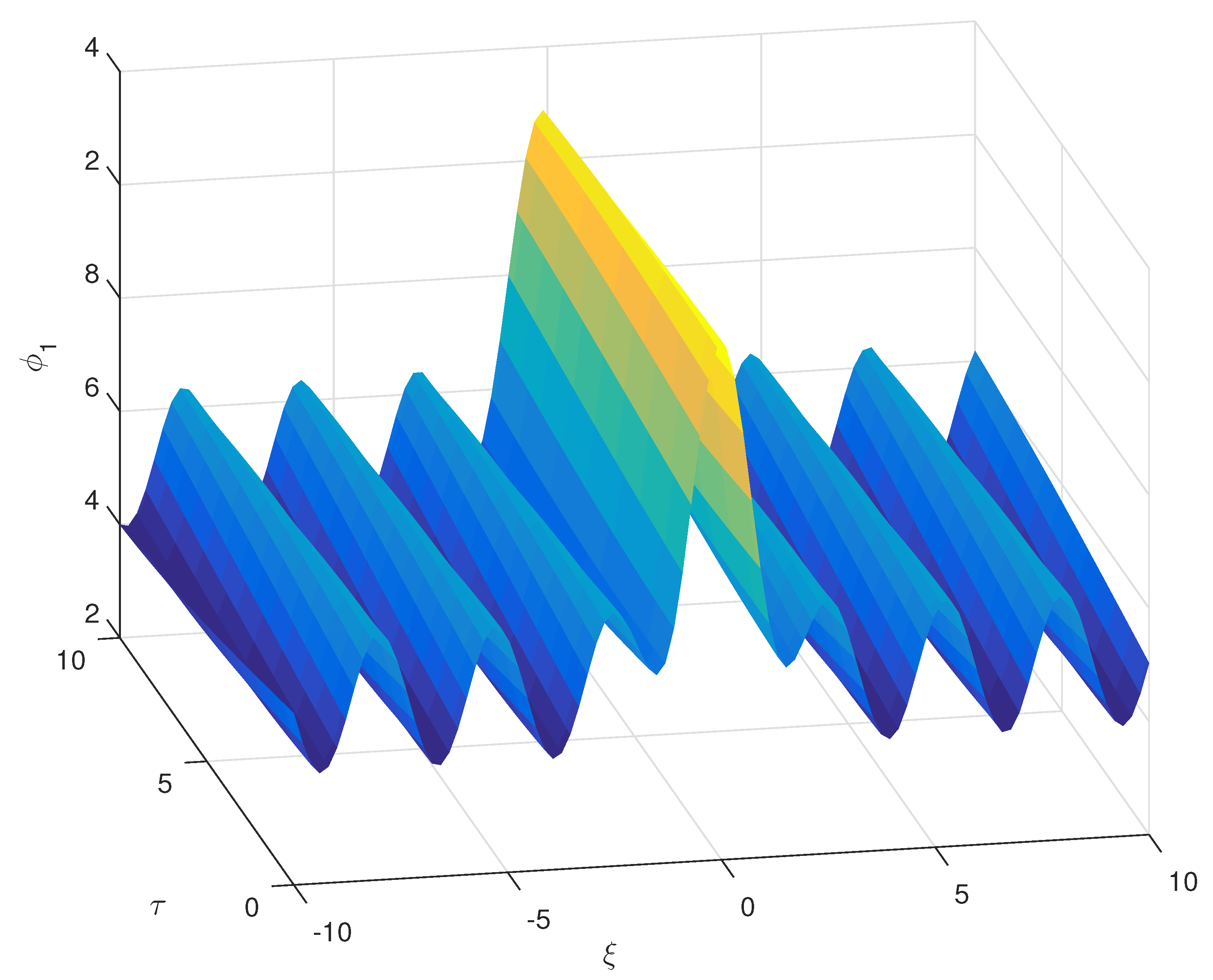
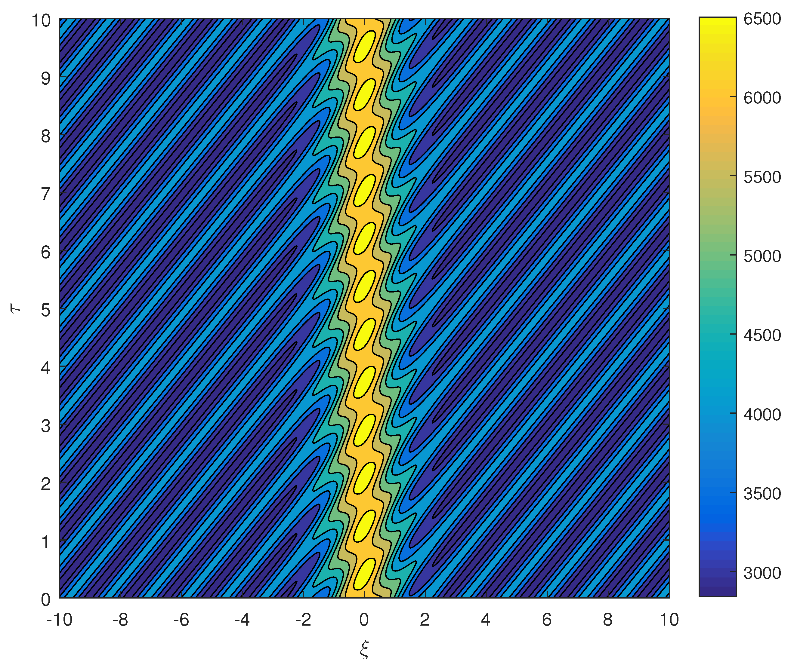
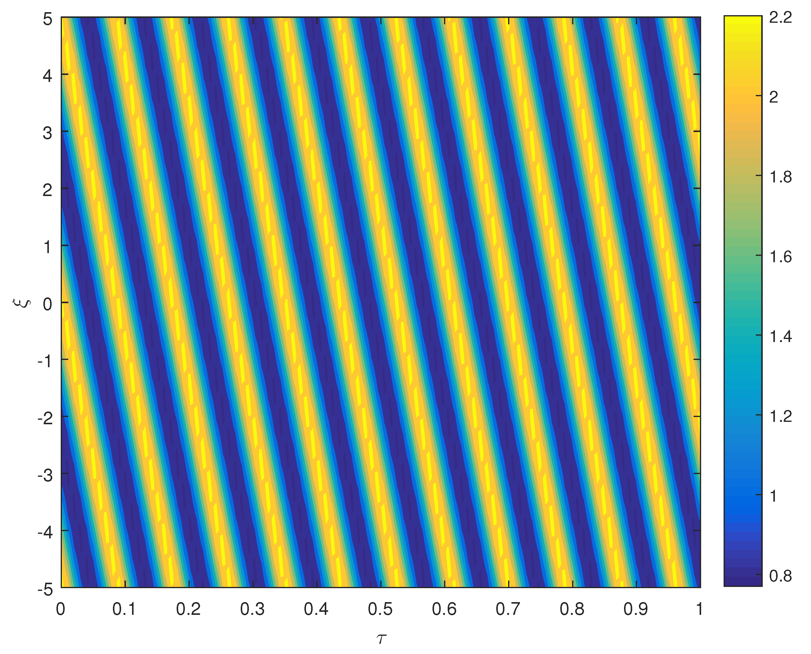
Moreover, in the Figure 11 we show the three dimensional form of this new wave form. Lastly, in Figure 12, we show a contour plot of ${\varphi }_1$ where the ordinate is time ‘$\tau$’ and the abscissa is ‘$\xi$’ for different parameter values.

5. Critical Nonlinearity and MKdv Equation

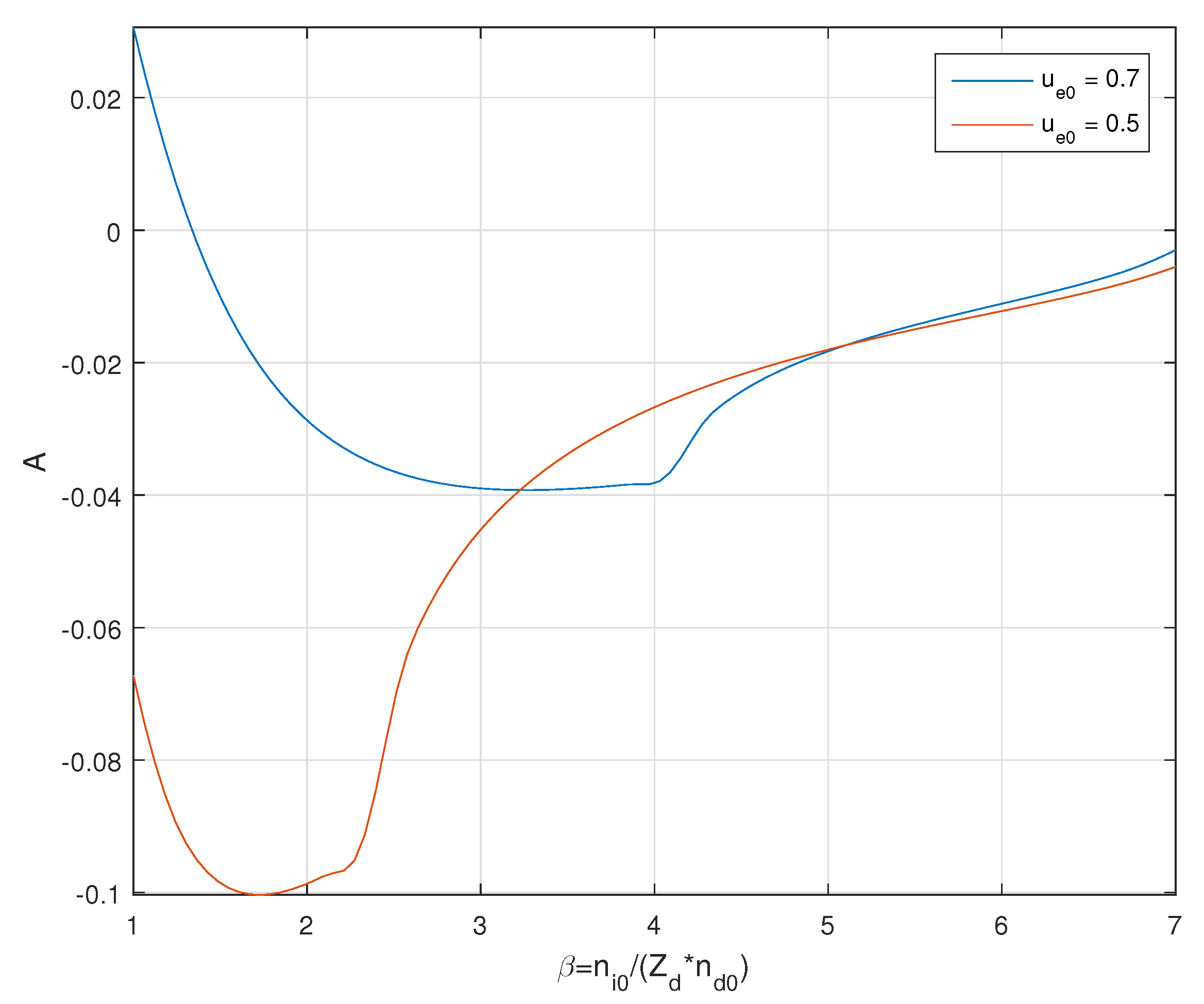
In the KdV equation derived in Equation (31) of Section 4, the nonlinear coefficient ‘A’ can vanish depending on the values of various parameters. In order to analyze this, we have plotted the form of ‘A’ as a function of $\beta =\left(\frac{n_{i0}}{Z_d{n}_{d0}}\right)$ depending on various values of the electron streaming velocities. In Figure 13 we have depicted this situation, where it is observed that, in presence of strong coupling, A can vanish for a particular situation.

In order to analyze such situations, we set the following.

$$\left.\begin{array}{c}\hfill \xi =ϵ(x-\lambda t)\\ \hfill \tau ={ϵ}^{3}t\end{array}\right\}$$

(38)

Since all the first order quantities remain the same. We only quote the second order and higher order perturbed quantities.

$$n_{e2}=\frac{u_{e2}}{\lambda -u_{e0}}+\frac{u_{e1}{n}_{e1}}{\lambda -u_{e0}}$$

(39)

$$u_{e2}=-\frac{{\alpha }_3/Z_d}{\lambda -u_{e0}}{\varphi }_2+\frac{u_{e1}^2/2}{\lambda -u_{e0}}$$

(40)

$$n_{d2}=\frac{u_{d2}}{\lambda }+\frac{u_{e1}{n}_{e1}}{\lambda }$$

(41)

$$u_{d2}=\frac{{\varphi }_2}{\lambda }+\frac{d_2}{\lambda }+\frac{d_1{n}_{d1}}{\lambda }+\frac{d_0{n}_{d2}}{\lambda }-\frac{u_{d1}^2}{\lambda }$$

(42)

$${\mu }_1{n}_{e2}+n_{d2}+\beta S{\varphi }_2-\beta S^2{\varphi }_1^2=0$$

(43)

which provides the following.

$${\varphi }_2=\frac{{\chi }_2}{{\chi }_1}{\varphi }_1^2$$

(44)

• ${\chi }_1=-\frac{{\alpha }_1{\mu }_1}{Z_d{(\lambda -u_{e0})}^2}+\frac{\lambda (d_{22}-1)}{[{\lambda }^2-(d_0+d_{11})]}+\beta$
• ${\chi }_2=\frac{3{\mu }_1{({\alpha }_1/Z_d)}^2}{2{(\lambda -u_{e0})}^4}+\frac{\lambda (d_{23}+d_{11}){(d_{12}-1)}^2}{{[{\lambda }^2-(d_0+d_{11})]}^3}+\frac{\lambda (d_{12}-1)(d_{12}+d_{24})}{{[{\lambda }^2-(d_0+d_{11})]}^2}+\frac{{(d_{12}-1)}^2}{{[{\lambda }^2-(d_0+d_{11})]}^2}+\frac{\lambda d_{25}}{[{\lambda }^2-(d_0+d_{11})]}-\beta$

However, from the next higher order terms in $ϵ$, we obtain the following:

$$-(\lambda -u_{e0})\frac{\partial n_{e3}}{\partial \xi }+\frac{\partial n_{e1}}{\partial \tau }+\frac{\partial u_{e3}}{\partial \xi }+\frac{\partial }{\partial \xi }\left(n_{e1}{u}_{e2}\right)+\frac{\partial }{\partial \xi }\left(n_{e2}{u}_{e1}\right)=0$$

(45)

$$-\lambda \frac{\partial n_{d3}}{\partial \xi }+\frac{\partial n_{e1}}{\partial \tau }+\frac{\partial u_{d3}}{\partial \tau }+\frac{\partial }{\partial \xi }\left(n_{d1}{u}_{d2}\right)+\frac{\partial }{\partial \xi }\left(n_{d2}{u}_{d1}\right)=0$$

(46)

$$\frac{\partial u_{e1}}{\partial \tau }-(\lambda -u_{e0})\frac{\partial u_{e3}}{\partial \xi }+\frac{\partial }{\partial \xi }\left(u_{e1}{u}_{e2}\right)={\alpha }_1{H}^2\frac{{\partial }^3{n}_{e1}}{\partial {\xi }^3}+\frac{{\alpha }_1}{Z_d}\frac{\partial {\varphi }_3}{\partial \xi }$$

(47)

$$\begin{array}{cc}\hfill & \frac{\partial u_{d1}}{\partial \tau }-\lambda \frac{\partial u_{d3}}{\partial \xi }+\frac{\partial }{\partial \xi }\left(u_{d1}{u}_{d2}\right)={\alpha }_1{H}^2\frac{{\partial }^3{n}_{d1}}{\partial {\xi }^3}+\hfill \\ & \frac{{\alpha }_1}{Z_d}\frac{\partial {\varphi }_3}{\partial \xi }-\frac{1}{Z_d}\frac{\partial d_3}{\partial \xi }-\frac{\partial }{\partial \xi }\left(d_2{n}_{d1}\right)-\frac{\partial }{\partial \xi }\left(d_1{n}_{d2}\right)-\hfill \\ & \left(\lambda -\frac{d_0}{\lambda }\right)\frac{\partial u_{d3}}{\partial \xi }-\frac{d_0}{\lambda }\left\{\frac{\partial n_{d1}}{\partial \tau }+\frac{\partial }{\partial \xi }\left(n_{d1}{n}_{d2}\right)+\frac{\partial }{\partial \xi }\left(n_{d2}{u}_{d1}\right)\right\}\hfill \end{array}$$

(48)

$$\frac{{\partial }^2{\varphi }_1}{\partial {\xi }^2}={\mu }_1{n}_{e3}+n_{d3}+\beta {\varphi }_3-2\beta {\varphi }_1{\varphi }_2$$

(49)

from which we can deduce

$$\frac{\partial {\varphi }_1}{\partial \tau }+A\frac{\partial }{\partial \xi }\left({\varphi }_1{\varphi }_2\right)+A^{\prime }\frac{\partial }{\partial \xi }\left({\varphi }_1^3\right)+B\frac{{\partial }^3{\varphi }_1}{\partial {\xi }^3}=0$$

(50)

which when $A\to 0$, it reduces to the M-KdV equation. The expression of the variable ‘$d_3$’ in Equation (48) is given as per Reference [24]. It is well known that the M-KdV equation also supports soliton solutions. However, here we found a new type of solution that is both solitonic and periodic in nature. For that we set the following:

$${\varphi }_1(\xi ,\tau )=U\left(s\right)$$

(51)

where $s=\xi +\omega \tau$. The second step is to choose $U\left(s\right)$ as follows:

$$\begin{array}{cc}\hfill & U\left(s\right)=g_0+\hfill \\ \hfill & \sum _{l=1}^M{\left(\frac{z\left(s\right)}{1+\left[z{\left(s\right)}^2\right]}\right)}^{(l-1)}\left(g_l\frac{z\left(s\right)}{1+{\left[z\left(s\right)\right]}^2}+f_l\frac{1-{\left[z\left(s\right)\right]}^2}{1+{\left[z\left(s\right)\right]}^2}\right)\hfill \end{array}$$

(52)

where $f_l$, $g_l$ are constants to be determined and $z\left(s\right)$ can be obtained as a solution of the following.

$${\left(\frac{dz\left(s\right)}{ds}\right)}^2=a+bz{\left(s\right)}^2+cz{\left(s\right)}^4$$

(53)

Several solutions of (53) are given in Reference [17], from which we have the following:

$${\varphi }_1(\xi ,\tau )=\pm \sqrt{\frac{3B}{2R}}\mp \frac{\sqrt{6B}}{R\sqrt{B/R}}\frac{1-c{n}^2(\eta ,\sqrt{3}/2)}{1+c{n}^2(\eta ,\sqrt{3}/2)}$$

(54)

where $\eta =\xi -\frac{5B}{2}\tau$.

On the other hand, for $\eta =\xi +\frac{5B}{2}\tau$, we can obtain the following.

$${\varphi }_1(\xi ,\tau )=\pm \sqrt{-\frac{3B}{2R}}\mp \frac{\sqrt{6B}}{R\sqrt{-3B/2R}}\frac{1-c{n}^2(\eta ,1/2)}{1+c{n}^2(\eta ,1/2)}$$

(55)

Here, ‘$cn$’ is the Jacobi elliptic Cosine function, $R=\frac{3{\chi }_2}{2{\chi }_1}A+3A^{\prime }$, where A and $A^{\prime }(=A_1^{\prime }/A_2)$ are given in Appendix A, and ${\chi }_1$ and ${\chi }_2$ are given after Equation (44). A diagrammatic representation of $A^{\prime }$ is given in Figure 14, while the graphical representation of the solution of Equation (54) is given in Figure 15 and Figure 16, which shows both a soliton and periodic behaviour. We have the used the same plasma parameters as in Section 4.1 for plotting these figures too.

6. Conclusions

In our above analysis, we have shown how an electron streaming in a quantum strongly coupled dusty plasma can generate both ‘slow’ and ‘fast’ modes in the plasma. Earlier this type of phenomenon was also studied by Shukla et al. [25] but that model did not take into account the quantum effects or strong coupling but the effect of the magnetic field. Though they have considered the streaming of ions, in our case the streaming of electrons have been taken into account since the electrons are light compared to that of ions or dust. These are then manifested as some nonlinear type of excitation in the ensuing KdV equations, which are a new type of solitonic solutions with periodic tails. Nowadays, such solutions are called ‘nanopteron’ solitons. Due to the role of various parameters and the electron streaming velocity, a critical situation can sometimes be arrived at where the nonlinear coefficient of the ‘KdV’ equation tends to zero. Here, we then take recourse to a modified scaling and the perturbation procedure, to arrive at the ‘MKdV’ equation. It is observed that the MKdV equation can also have a new type of nonlinear excitation, which reflects both a solitonic and periodic nature at the same time. The whole process is surely influenced by the strength of the strong coupling and other parameters. It may be added that the nature of the strong coupling force in the form of the potential was discussed in References [23,26] and calculated in detail in Reference [23].