Computing the Double-Gyroaverage Term Incorporating Short-Scale Perturbation and Steep Equilibrium Profile by the Interpolation Algorithm

Abstract

In the gyrokinetic model and simulations, when the double-gyroaverage term incorporates the combining effect contributed by the finite Larmor radius, short scales of the perturbation, and steep gradient of the equilibrium profile, the low-order approximation of this term could generate unignorable error. This paper implements an interpolation algorithm to compute the double-gyroaverage term without low-order approximation to avoid this error. For a steep equilibrium density, the obvious difference between the density on the gyrocenter coordinate frame and the one on the particle coordinate frame should be accounted for in the quasi-neutrality equation. A Euler–Maclaurin-based quadrature integrating algorithm is developed to compute the quadrature integral for the distribution of the magnetic moment. The application of the interpolation algorithm to computing the double-gyroaverage term and to solving the quasi-neutrality equation is benchmarked by comparing the numerical results with the known analytical solutions. Finally, to take advantage of the interpolation solver clearer, the numerical comparison between the interpolation solver and a classical second order solver is carried out in a constant theta-pinch magnetic field configuration using SELALIB code. When the equilibrium profile is not steep and the perturbation only has the non-zero mode number along the parallel spatial dimension, the results computed by the two solvers match each other well. When the gradient of the equilibrium profile is steep, the interpolation solver provides a bigger driving effect for the ion-temperature-gradient modes, which possess large polar mode numbers.

1. Introduction

Micro-scale turbulence plays a significant role in the confinement capability of magnetized fusion plasma through its interaction with low-frequency zonal flow [1,2,3,4,5,6,7], equilibrium profile at the pedestal region, and edge localized modes [8,9,10,11,12], etc. The importance of the pedestal region is reflected by the fact that the pressure of the plasma core is proportional to the pressure at the pedestal top [13,14,15]. The gradient of the equilibrium temperature and density at the pedestal region could be very sharp; alternatively, the truncation of $exp({\mathit{\rho }}_0·\nabla )$ acting over $n_0$ or $T_0$ at the first order, which is used by the standard gyrokinetic model [16,17,18], is not a good approximation, where ${\mathit{\rho }}_0$ is the Larmor radius vector defined as

$${\mathbf{\rho }}_0(\mathbf{x},\mu ,\theta )=\frac{1}{q_s}\sqrt{\frac{2\mu m_s}{B}}\left({\mathbf{e}}_{1}cos\theta +{\mathbf{e}}_{2}sin\theta \right).$$

Here, $q_s,m_s,\mu$ are the particles’ charge, mass, and the magnetic moment on the guiding-center coordinate frame; ${\mathbf{e}}_1,{\mathbf{e}}_2$ are the unit vectors perpendicular to unit vector $\mathbf{b}$ of the equilibrium magnetic field, and ${\mathbf{e}}_1,{\mathbf{e}}_2,\mathbf{b}$ obey the right-hand rule; B is the magnitude of the magnetic field; $\theta$ is the gyrophase angle; $n_0,T_0$ are the equilibrium density and temperature profile. In gyrokinetic theory, the first gyroaverage term could incorporate the effect contributed by the finite Larmor radius and short scales of the perturbation at the core and edge tokamak plasma, while the double-gyroaverage term (DGT) incorporates the combining effect contributed by the finite Larmor radius, the short-scale perturbation and the steep-gradient equilibrium profile within the edge transport barrier of tokamak plasma [18,19,20,21]. However, in the standard electrostatic gyrokinetic model and simulations, the approximation of DGT consists of up to the first order truncation of the Taylor expansion of the equilibrium profile and the second order truncation of the expansion of the perturbative potential [16,17,22,23,24,25,26,27,28]. The details of this method can be found in Appendix A. These kinds of low-order approximation are not sufficient concerning the short-scale perturbations and the equilibrium profile possessing the steep gradient.

To overcome the mentioned drawbacks of the low-order approximation of DGT, this paper develops an interpolation algorithm to compute DGT for the purpose of the resolving of the short-scale perturbation and the steep equilibrium profile together. The interpolation algorithm can approach DGT with arbitrary accuracy by choosing enough sampling points on the Larmor circle, with only the constraint from the length scale of the mesh. Meanwhile, contrary to the traditional way, the steep equilibrium density profile should not keep the same before and after the gyroaverage operation, which is denoted by the symbol $\mathcal{J}$ in this paper. And the obvious difference between the density on gyrocenter coordinate and the one on the particle coordinates should be accounted for in the quasi-neutrality equation(QNE). The obvious difference is revealed by Figure 1, for which the normalization scheme can be found in Section 3.3 and the parameters to obtain this figure are provided in Section 7.3.3. In Figure 1, the purple line denotes the equilibrium density profile on the gyrocenter coordinates, which is given as the initial condition, while the density profiles on the particle coordinate derived by the gyroaverage operation computed with different number of $\mu$ are shown by other curves. The numerical integration of $\mu$ is done by the Euler–Maclaurin-based quadrature integration algorithm.

As a comparison to the interpolation solver, a classical 2nd order truncation of DGT is carried out in this paper to obtain QNE with the 2nd-order accuracy. It consists of the truncation of the exponential operator $exp({\mathit{\rho }}_0·\nabla )$ over the potential up to the second order and the truncation of the operator $exp({\mathit{\rho }}_0·\nabla )$ acting on the density up to the first order. The numerical simulations are carried out to compare the two solvers. Since this paper is to compare the two solvers in general purpose, the deduction of flux-surface average of the potential from the total potential is not carried out to obtain the electrons’ adiabatic distribution. For the equilibrium profile without steep gradient, both algorithms have almost the same performance in terms of the perturbation only possessing the mode number along the parallel spatial dimension. For the steep equilibrium profile, the interpolation algorithm could provide a stronger driving effect for the perturbation of high polar mode numbers, and the saturation time of these modes computed by the interpolation algorithm is earlier.

The remaining parts of this paper are arranged as follows. Section 2 introduces the orders used in deriving the gyrokinetic model. The DGT and QNE incorporating the short-scale perturbation and steep equilibrium profile on the gyrocenter coordinate frame are derived in Section 3. In Section 4, the interpolation solver is introduced. The benchmark of the interpolation algorithm is done in Section 5 and Section 6 for the case of the single $\mu$ and $\mu$ obeying the distribution, respectively. The Euler–Maclaurin-based quadrature integrating algorithm is developed in Section 6 to compute the numerical quadrature integral of $\mu$. The application of the interpolation algorithm and the Euler–Maclaurin-based quadrature integrating algorithm to the gyrokinetic simulations is provided by Section 7, where the parallel scheme of the whole simulations is presented.

2. The Basic Orders

There are several basic orders or scales contained by the perturbation. The first one is the length scale $O\left(\epsilon \right)$ of the nondimensionalized Larmor radius being $\epsilon$. The second one is the amplitude of the normalized electrostatic potential, whose $\epsilon$-based order is denoted as $O\left({\epsilon }^{\sigma }\right)$ with the power $\sigma$ a positive real number. In the magnetically confined fusion plasmas, because the charged particle can nearly migrate freely in the environment with collective interactions, the magnitude of the potential the particles feel must be much smaller than that of its kinetic energy.

The third one is the length scale of the gradient of the electrostatic potential. Define ${\mathcal{K}}_{\perp }\equiv |\frac{{\nabla }_{\perp }\varphi }{\varphi }|$ and ${\mathcal{K}}_{\parallel }\equiv |\frac{{\nabla }_{\parallel }\varphi }{\varphi }|$, where the subscript ⊥ and ∥ denotes the directions perpendicular and parallel the direction of equilibrium magnetic field, respectively. The gyrokinetic model of this paper adopts the scales for the perturbation

$$O\left(\epsilon {\mathcal{K}}_{\perp }\right)=O\left(1\right),O\left(\epsilon {\mathcal{K}}_{\parallel }\right)=O\left(\epsilon \right),$$

(1)

where the short scales of the perturbation are accounted for. For any equilibrium quantity $\mathcal{E}\in \{n_0,T_0\}$, this paper considers the scale

$$O\left(\epsilon \parallel \frac{{\nabla }_{\perp }\mathcal{E}}{\mathcal{E}}\parallel \right)=O\left(1\right),$$

(2)

due to the steep gradient of the equilibrium profiles, as well as the following scales

$$O\left(\epsilon \parallel \frac{{\nabla }_{\parallel }\mathcal{E}}{\mathcal{E}}\parallel \right)=O\left(\epsilon \right),O\left(\epsilon \parallel \frac{{\partial }_U\mathcal{E}}{\mathcal{E}}\parallel \right)=O\left(\epsilon \right),$$

where U is the parallel velocity and will be given later.

3. QNE Incorporating the Short-Scale Perturbation and Steep Equilibrium Profile

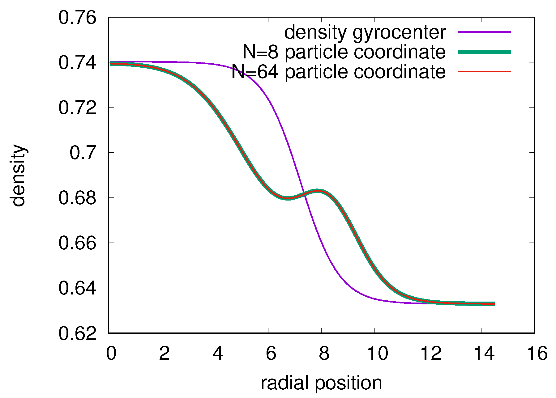
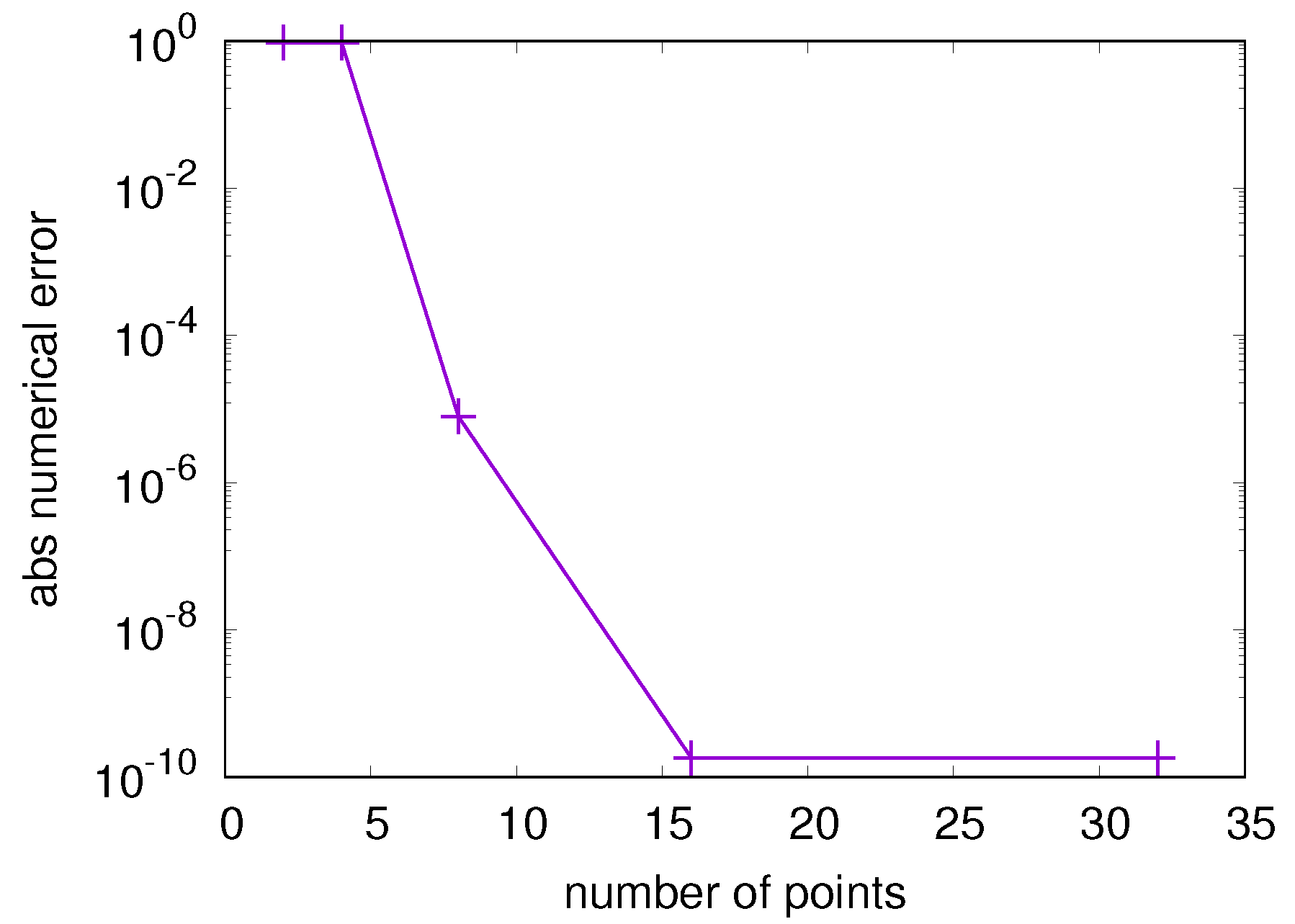
3.1. The Particle Coordinate Density Associated with the Short-Scale Perturbation and Steep Equilibrium Profile

The procedure to derive the gyrokinetic model is composited by two parts. The first one is to derive the coordinate transform by decoupling the gyroangle from the dynamics of the remaining variables, while the second one is to obtain the gyrokinetic quasi-neutrality equation by inducing the transformation of the distribution through the derived coordinate transforms [16,19,29,30]. The first step is accomplished by implementing Lie transform perturbation method on the fundamental Lagrangian one-form. Generally, four kinds of coordinate frameworks are involved in the procedure. The first one is the full-orbit coordinate with the velocity part in Cartesian coordinates. it is denoted as $\overline{\mathbf{z}}\equiv (\mathbf{x},\mathbf{v})$ here. The second one is obtained by transforming $\mathbf{v}$ into the cylindrical coordinates, and it is written as $\mathbf{z}\equiv (\mathbf{x},{\mu }_1,u_1,{\theta }_1)$ where ${\mu }_1\equiv \frac{m{v}_{\perp }^2}{2B\left(\mathbf{x}\right)}$, $u_1$ is the velocity along the parallel direction, and ${\theta }_1$ is the angle between $\mathit{\rho }$ and ${\mathbf{e}}_1$. The $\mathbf{x}$ component in $\mathbf{z}$ is still in full-orbit frame. The third one is the guiding-center coordinates $\overline{\mathbf{Z}}=(\overline{\mathbf{X}},\overline{\mu },\overline{U},\overline{\theta })$, which is derived by decoupling $\overline{\theta }$ from the dynamics of the other coordinate components without the presence of the perturbation. The fourth one is the gyrocenter coordinate $\mathbf{Z}=(\mathbf{X},\mu ,U,\theta )$ which is derived by decoupling $\overline{\theta }$ from the dynamics of the other coordinate components with the presence of the perturbation. The coordinate transforms between $\overline{\mathbf{z}}$, $\mathbf{z}$,$\overline{\mathbf{Z}}$ and $\mathbf{Z}$ are denoted as ${\psi }_f:\overline{\mathbf{z}}\to \mathbf{z}$, ${\psi }_{gc}:\mathbf{z}\to \overline{\mathbf{Z}}$ and ${\psi }_{gy}:\overline{\mathbf{Z}}\to \mathbf{Z}$, respectively, while the distributions on the four kinds of coordinates are respectively written as $\overline{f}\left(\overline{\mathbf{z}}\right)$, $f\left(\mathbf{z}\right)$, $\overline{F}\left(\overline{\mathbf{Z}}\right)$ and $F\left(\mathbf{Z}\right)$.

The coordinate transform ${\psi }_{gc}:\mathbf{z}\to \overline{\mathbf{Z}}$ is given by

$$\begin{array}{ccc}\hfill \overline{\mathbf{X}}& =& \mathbf{x}-{\mathbf{\rho }}_0(\mathbf{x},{\mu }_1,{\theta }_1),\hfill \end{array}$$

(3a)

$$\begin{array}{ccc}\hfill \overline{\mu }& =& {\mu }_1,\hfill \end{array}$$

(3b)

$$\begin{array}{ccc}\hfill \overline{U}& =& u_1,\hfill \end{array}$$

(3c)

$$\begin{array}{ccc}\hfill \overline{\theta }& =& {\theta }_1.\hfill \end{array}$$

(3d)

while the coordinate transform ${\psi }_{gy}:\overline{\mathbf{Z}}\to \mathbf{Z}$ is provided by the following equations

$$\begin{array}{ccc}\hfill \mathbf{X}& =& \overline{\mathbf{X}},\hfill \end{array}$$

(4a)

$$\begin{array}{ccc}\hfill \mu & =& \overline{\mu }+g_2^{\mu }\left(\overline{\mathbf{X}},\overline{\mu },\overline{\theta }\right),\hfill \end{array}$$

(4b)

$$\begin{array}{ccc}\hfill U& =& \overline{U},\hfill \end{array}$$

(4c)

$$\begin{array}{ccc}\hfill \theta & =& \overline{\theta }+g_2^{\theta }\left(\overline{\mathbf{X}},\overline{\mu },\overline{\theta }\right).\hfill \end{array}$$

(4d)

where

$$\begin{array}{ccc}\hfill g_2^{\mu }\left(\overline{\mathbf{X}},\overline{\mu },\overline{\theta }\right)& =& \frac{q_s\mathsf{\Psi }\left(\overline{\mathbf{X}},\overline{\mu },\overline{\theta }\right)}{B\left(\overline{\mathbf{X}}\right)},\hfill \end{array}$$

(5a)

$$\begin{array}{ccc}\hfill g_2^{\theta }\left(\overline{\mathbf{X}},\overline{\mu },\overline{\theta }\right)& =& \frac{q_s{\partial }_{\overline{\mu }}{\int }_0^{\overline{\theta }}\mathsf{\Psi }\left(\overline{\mathbf{X}},\overline{\mu },\overline{\theta }\right)d\overline{\theta }}{B\left(\overline{\mathbf{X}}\right)},\hfill \end{array}$$

(5b)

and

$$\begin{array}{ccc}\hfill \mathsf{\Psi }\left(\overline{\mathbf{X}},\overline{\mu }\right)& \equiv & \varphi \left(\overline{\mathbf{X}}+{\mathbf{\rho }}_0\right)-\mathsf{\Phi }(\overline{\mathbf{X}},\overline{\mu }),\hfill \end{array}$$

(6a)

$$\begin{array}{ccc}\hfill \mathsf{\Phi }(\overline{\mathbf{X}},\overline{\mu })& \equiv & \frac{1}{2\pi }{\int }_0^{2\pi }\varphi \left(\overline{\mathbf{X}}+{\mathbf{\rho }}_0\right)d\theta ,\hfill \end{array}$$

(6b)

$$\begin{array}{ccc}\hfill {\mathbf{\rho }}_0(\overline{\mathbf{X}},\overline{\mu },\overline{\theta })& =& \frac{1}{q_s}\sqrt{\frac{2\overline{\mu }{m}_s}{B}}\left({\mathbf{e}}_{1}cos\overline{\theta }+{\mathbf{e}}_{2}sin\overline{\theta }\right).\hfill \end{array}$$

(6c)

And through the Lie transform perturbative method, we could derive the following Lagrangian on the gyrocenter coordinate frame

$$\mathcal{L}=\left(q_s\mathbf{A}\left(\mathbf{X}\right)+m_{s}U\mathbf{b}\right)·\dot{\mathbf{X}}+\frac{m_s}{q_s}\mu \dot{\theta }-\left(\mu B\left(\mathbf{X}\right)+\frac{m_s{U}^2}{2}+\mathsf{\Phi }(\mathbf{X},\mu )\right),$$

(7)

where $\mu$ is a constant. The Euler-Lagrangian equations based on $\mathcal{L}$ in Equation (7) provides the equations of motion as follows:

$$\begin{array}{ccc}\hfill \stackrel{.}{\mathbf{X}}& =& \frac{q_{s}U{\mathbf{B}}^{\ast }-\mathbf{b}\times \nabla \left(\mu B+q_s\mathsf{\Phi }(\mathbf{X},\mu )\right)}{q_s{B}_{\parallel }^{\ast }},\hfill \end{array}$$

(8a)

$$\begin{array}{ccc}\hfill \dot{U}& =& \frac{{\mathbf{B}}^{\ast }·\nabla \left(\mu B+q_s\mathsf{\Phi }(\mathbf{X},\mu )\right)}{m_s{B}_{\parallel }^{\ast }},\hfill \end{array}$$

(8b)

where ${\mathbf{B}}^{\ast }=\mathbf{B}+\frac{m_s}{q_s}U\nabla \times \mathbf{b}$. If the denominate in Equation (8a) is expanded by the order of the small factor $\frac{m_s}{q_s}U\nabla \times \mathbf{b}$, we could obtain the curvature drift part $\frac{m{U}^2\kappa }{eB}$ where $\kappa =\frac{\nabla B}{B}$.

For the Vlasov gyrokinetic simulation, we need to transform the distribution function from the gyrocenter coordinate to the full-orbit coordinate [16]. After obtaining the coordinate transform composited by Equations (3a)–(3d) and (4a)–(4d), given a distribution function on the gyrocenter coordinate $F_s\left(\mathbf{X},\mu ,U,t\right)$, the distribution function on the full orbit can be derived following the transform chain

$$F_s\left(\mathbf{X},\mu ,U\right)\stackrel{{\psi }_{gy}}{⟶}{\overline{F}}_s\left(\overline{\mathbf{Z}}\right)\stackrel{{\psi }_{gc}}{⟶}{f}_s\left(\mathbf{z}\right).$$

(9)

First, the total distribution function is separated into the sum of an equilibrium one plus a perturbative one as

$$F_s\left(\mathbf{X},\mu ,U\right)=F_{s0}\left(\mathbf{X},\mu ,U\right)+F_{s1}\left(\mathbf{X},\mu ,U\right).$$

(10)

Then, the approximation of the distribution on the guiding-center coordinate can be derived based on the coordinate transform given by Equations (4a)–(4d)

$$\begin{array}{cc}\hfill {\overline{F}}_s\left(\overline{\mathbf{Z}}\right)& =F_s\left(\overline{\mathbf{X}},\overline{\mu }+g_2^{\mu }\left(\overline{\mathbf{X}},\overline{\mu },\overline{\theta }\right),\overline{U}\right)\hfill \\ & \approx F_s\left(\overline{\mathbf{X}},\overline{\mu },\overline{U}\right)+\frac{q_s\mathsf{\Psi }\left(\overline{\mathbf{Z}}\right)}{B\left(\overline{\mathbf{Z}}\right)}{\partial }_{\overline{\mu }}{F}_{s0}\left(\overline{\mathbf{X}},\overline{\mu },\overline{U}\right)\hfill \\ & =F_s\left(\overline{\mathbf{X}},\overline{\mu },\overline{U}\right)-\frac{q_s\mathsf{\Psi }\left(\overline{\mathbf{Z}}\right)}{T_s\left(\overline{\mathbf{Z}}\right)}{F}_{s0}\left(\overline{\mathbf{X}},\overline{\mu },\overline{U}\right),\hfill \end{array}$$

(11)

where the equilibrium distribution involving $\mu$ is assumed as

$$F_{s0\perp }=\frac{m_s}{2\pi T_s}exp(-\frac{\mu B}{T_s}).$$

(12)

The approximation of $f_s\left(\mathbf{z}\right)$ is derived with Equation (11) as the base

$$\begin{array}{cc}\hfill f_s\left(\mathbf{z}\right)& =F_s\left(\mathbf{x}-{\mathbf{\rho }}_0\left(\mathbf{x},{\mu }_1,{\theta }_1\right),{\mu }_1,u_1\right)-q_s\frac{\varphi \left(\mathbf{x}\right)F_{s0}(\mathbf{x}-{\mathbf{\rho }}_0\left(\mathbf{x},{\mu }_1,{\theta }_1\right),{\mu }_1,u_1)}{T_s\left(\mathbf{x}\right)}\hfill \\ & +q_s\left(\frac{\mathsf{\Phi }{F}_{s0}}{T_s}\right)\left(\mathbf{x}-{\mathbf{\rho }}_0\left(\mathbf{x},{\mu }_1,{\theta }_1\right),{\mu }_1,u_1\right).\hfill \end{array}$$

(13)

where $\left(\frac{\mathsf{\Phi }{F}_{s0}}{T_s}\right)\left(\mathbf{x}-{\mathit{\rho }}_0\left(\mathbf{x},{\mu }_1,{\theta }_1\right),{\mu }_1,u_1\right)$ is the origin of DGT and comprises the effect combining together the finite Larmor radius, short-scale perturbation, and steep equilibrium profile.

We assume that the equilibrium distribution $F_{s0}$ can be decomposed as the product between the parallel part and the perpendicular part

$$F_{s0}(\mathbf{x},{\mu }_1,u_1)=n_0\left(\mathbf{x}\right)F_{s0\parallel }\left(\mathbf{x},u_1\right)F_{s0\perp }\left(\mathbf{x},{\mu }_1\right),$$

(14)

with probability conservation satisfied by

$$\begin{array}{ccc}\hfill \int F_{s0\parallel }d{u}_1& =& 1,\hfill \end{array}$$

(15a)

$$\begin{array}{ccc}\hfill \int F_{s0\perp }\frac{B\left(\mathbf{x}\right)}{m_s}d{\mu }_{1}d{\theta }_1& =& 1,\hfill \end{array}$$

(15b)

where under the equilibrium condition, the metric $B\left(\mathbf{x}\right)/m_s$ is used.

Then, through the integral $n_s\left(\mathbf{x},t\right)=\int f_s\left(\mathbf{z}\right)\frac{B\left(\mathbf{x}\right)}{m_s}d{\mu }_{1}d{u}_{1}d{\theta }_1$, the density can be assembled as

$$n_s\left(\mathbf{x}\right)=n_{sg0}\left(\mathbf{x}\right)-q_s\frac{n_{sg0}\varphi }{T_s}+q_s{\tilde{\varphi }}^{\prime }\left(\mathbf{x}\right)+n_{sg1}\left(\mathbf{x},t\right),$$

(16)

with

$$\begin{array}{ccc}\hfill n_{sg0}\left(\mathbf{x}\right)& =& \int F_{s0}\left(\mathbf{x}-{\mathbf{\rho }}_0\left(\mathbf{z}\right),{\mu }_1,u_1\right)\frac{B\left(\mathbf{x}\right)}{m_s}d{\mu }_{1}d{u}_{1}d{\theta }_1,\hfill \end{array}$$

(17a)

$$\begin{array}{ccc}\hfill n_{sg1}\left(\mathbf{x},t\right)& =& \int F_{s1}\left(\mathbf{x}-{\mathbf{\rho }}_0\left(\mathbf{z}\right),{\mu }_1,u_1\right)\frac{B\left(\mathbf{x}\right)}{m_s}d{\mu }_{1}d{u}_{1}d{\theta }_1,\hfill \end{array}$$

(17b)

$$\begin{array}{ccc}\hfill {\tilde{\varphi }}^{\prime }\left(\mathbf{x}\right)& =& \int \left(\frac{\mathsf{\Phi }{F}_{s0}}{T_s}\right)\left(\mathbf{x}-{\mathbf{\rho }}_0,{\mu }_1,u_1\right)\frac{B\left(\mathbf{x}\right)}{m_s}d{\mu }_{1}d{u}_{1}d{\theta }_1.\hfill \end{array}$$

(17c)

Here, the metric $B\left(\mathbf{x}\right)/m_s$ of the phase space is used.

3.2. QNE Associated with the Adiabatic Distribution of Electron and the Steep Equilibrium Profile on Gyrocenter Coordinate Frame

As shown in Figure 1, the equilibrium density profile possessing the steep gradient on the gyrocenter coordinate frame is obviously different from the one on the particle coordinate frame after the gyroaverage operation. Therefore, contrary to the traditional way, the implementation of the equilibrium density on the particle coordinate frame should be different from the one on the gyrocenter coordinate frame if its profile is steep in the radial dimension.

We consider a plasma only including protons and electrons. The electrons obey the adiabatic distribution on the particle coordinate space

$$n_e\left(\mathbf{x}\right)=n_{g0}\left(\mathbf{x}\right)+\frac{e{n}_{g0}\left(\mathbf{x}\right)}{T_e}\varphi \left(\mathbf{x}\right),$$

(18)

where the flux-surface average of the potential is not deducted from the total potential, because our purpose is to compare the two solvers. $n_{g0}\left(\mathbf{x}\right)$ is the equilibrium density in the particle coordinate space and needs to be solved. The initial equilibrium distribution of ion is given on the guiding-center coordinate system by

$$F_{i0}(\mathbf{x},\mu ,U)=\frac{n_0\left(\mathbf{x}\right)}{{\left(2\pi T_i\left(\mathbf{x}\right)\right)}^{3/2}}exp(-\frac{U^2}{2T_i\left(\mathbf{x}\right)}-\frac{\mu B\left(\mathbf{x}\right)}{T_i\left(\mathbf{x}\right)}),$$

from which the equilibrium density on the guiding-enter coordinate is easily derived as $n_0\left(\mathbf{x}\right)$. For the scales given by Equation (2), the equilibrium density on the particle coordinate space should be derived as

$$n_0^{\prime }=\int F_{i0}(\mathbf{x}-{\mathbf{\rho }}_0,\mu ,U)\frac{B}{m_i}d{\mu }_{1}dUd\theta$$

(19)

Taking into account of the quasi-neutrality equilibrium, it is derived that

$$n_{g0}\left(\mathbf{x}\right)=n_0^{\prime }\left(\mathbf{x}\right).$$

(20)

Then, QNE of this plasma is

$$\frac{e\varphi }{T_i}-\frac{e{\tilde{\varphi }}^{\prime }}{n_{g0}}+\frac{e\varphi }{T_e}=\frac{n_{i1}}{n_{g0}}.$$

(21)

3.3. Normalization

In this paper, the quantities $t,v,B,l,\mu ,T,\varphi$ are normalized by $t_0\equiv \frac{m}{B_0{q}_i}$, $v_0\equiv \sqrt{\frac{T_{e0}}{m_i}}$, $B_0$, $l_0\equiv \frac{m{v}_0}{e{B}_0}$, ${\mu }_0\equiv \frac{T_{e0}}{B_0}$, $T_{e0}$ and ${\varphi }_0\equiv \frac{T_{e0}}{q_i}$, respectively, where $T_{e0}\equiv T_e\left(r_p\right)$ and $r_p\in [r_{min},r_{max}]$ is the radial position of the peak of the initial distribution function. Then, by choosing the equilibrium perpendicular distribution given by Equation (12), the normalized QNE is

$$\frac{\varphi \left(\mathbf{x}\right)}{T_i\left(\mathbf{x}\right)}-\frac{\tilde{\mathsf{\Phi }}\left(\mathbf{x}\right)}{n_{g0}\left(\mathbf{x}\right)}+\frac{\varphi \left(\mathbf{x}\right)}{T_e\left(\mathbf{x}\right)}=\frac{n_{i1}\left(\mathbf{x}\right)}{n_{g0}\left(\mathbf{x}\right)},$$

(22)

with the normalized DGT

$$\tilde{\mathsf{\Phi }}\left(\mathbf{x}\right)=\int \left(\frac{\mathsf{\Phi }{F}_{i0}}{T_i}\right)\left(\mathbf{x}-{\mathbf{\rho }}_0,{\mu }_1,u_1\right)B\left(\mathbf{x}\right)d{\mu }_{1}d{u}_{1}d{\theta }_1,$$

(23)

and $F_0=\frac{n_0\left(r\right)exp\left(-\frac{U^2}{2T_i\left(r\right)}-\frac{\mu B}{T_i\left(r\right)}\right)}{{\left(2\pi T_i\left(r\right)\right)}^{3/2}}$.

4. QNE Solver Comprising the Interpolation Algorithm to Compute DGT

4.1. The Algorithm to Compute the Interpolation Matrixes $A^{spl}$ and $A_{l,{\rho }_j}^{contr}$ in Finite Element Method

In this paper, we sometimes use the symbols ${\mathcal{J}}_1\left(\mu \right)$ and ${\mathcal{J}}_2\left(\mu \right)$ to denote the first and the second gyroaverage associated with the magnetic moment $\mu$, specifically,

$${\mathcal{J}}_1\left(\mu \right)\varphi \left(\mathbf{x}\right)=\frac{1}{2\pi }\int \varphi (\mathbf{x}+{\mathbf{\rho }}_0\left(\mu \right))d\theta ,$$

$${\mathcal{J}}_2\left(\mu \right)\varphi \left(\mathbf{x}\right)=\frac{1}{2\pi }\int \varphi (\mathbf{x}-{\mathbf{\rho }}_0\left(\mu \right))d\theta .$$

In our interpolation scheme of the finite element method(FEM), the following cubic spline function is used as the basis function

$$B_{\alpha }\left(x\right)=\frac{1}{6h^3}\left\{\begin{array}{cc}{(x-x_{\alpha -2})}^3\hfill & \mathrm{if}{x}_{\alpha -2}\le x\le x_{\alpha -1}\hfill \\ h^3+3h^2(x-x_{\alpha -1})+3h{(x-x_{\alpha -1})}^2-3{(x-x_{\alpha -1})}^3\hfill & \mathrm{if}{x}_{\alpha -1}\le x\le x_{\alpha }\hfill \\ h^3+3h^2(x_{\alpha +1}-x)+3h{(x_{\alpha +1}-x)}^2-3{(x_{\alpha +1}-x)}^3\hfill & \mathrm{if}{x}_{\alpha }\le x\le x_{\alpha +1}\hfill \\ {(x_{\alpha +2}-x)}^3\hfill & \mathrm{if}{x}_{\alpha +1}\le x\le x_{\alpha +2}\hfill \\ 0\hfill & \mathrm{otherwise}\hfill \end{array}\right.$$

The spatial domains $(x,y,z)$, where z is the coordinate parallel to the equilibrium magnetic unit vector, the parallel velocity U and the magnetic moment $\mu$ are equally discretized.

To obtain the matrix form, the physical quantities on the grid mesh are written in the vectors as follows:

$$\begin{array}{ccc}\hfill {\psi }_{h,p}& :=& \psi (x_h,y_p),h\in \{0,\cdots ,N_x\};p\in \{0,\cdots ,N_y-1\}\hfill \\ \hfill {\psi }_{h,p,j}& :=& \psi (x_h,y_p,{\mu }_j),j\in \{1,\cdots ,N_{\mu }\}\hfill \\ \hfill {\psi }_{h,p,jk}& :=& \psi (x_h,y_p,{\mu }_j,U_k),k\in \{1,\cdots ,N_U\}\hfill \\ \hfill \varphi & :=& {({\varphi }_{0,0},\cdots ,{\varphi }_{N_x,0},{\varphi }_{0,1},\cdots ,{\varphi }_{N_x,1},\cdots ,{\varphi }_{0,N_y-1},\cdots ,{\varphi }_{N_x,N_y-1})}^t,\hfill \\ \hfill {\mathsf{\Phi }}_j& :=& {({\mathsf{\Phi }}_{0,0,j},\cdots ,{\mathsf{\Phi }}_{N_x,0,j},{\mathsf{\Phi }}_{0,1,j},\cdots ,{\mathsf{\Phi }}_{N_x,1,j},\cdots ,{\mathsf{\Phi }}_{0,N_y-1,j},\cdots ,{\mathsf{\Phi }}_{N_r,N_y-1,j})}^t,\hfill \\ \hfill {\mathcal{F}}_{sjk}& :=& {({\mathcal{F}}_{0,0,jk},\cdots ,{\mathcal{F}}_{N_x,0,jk},{\mathcal{F}}_{0,1,jk},\cdots ,{\mathcal{F}}_{N_x,1,jk},\cdots ,{\mathcal{F}}_{0,N_y-1,jk},\cdots ,{\mathcal{F}}_{N_x,N_y-1,j})}^t,\hfill \\ \hfill {\overline{\mathsf{\Phi }}}_{jk}& :=& {({\overline{\mathsf{\Phi }}}_{0,0,jk},\cdots ,{\overline{\mathsf{\Phi }}}_{N_x,0,jk},{\overline{\mathsf{\Phi }}}_{0,1,jk},\cdots ,{\overline{\mathsf{\Phi }}}_{N_x,1,jk},\cdots ,{\overline{\mathsf{\Phi }}}_{0,N_y-1,jk},\cdots ,{\overline{\mathsf{\Phi }}}_{N_x,N_y-1,jk})}^t,\hfill \\ \hfill {\tilde{\mathsf{\Phi }}}_{jk}& :=& {({\tilde{\mathsf{\Phi }}}_{0,0,jk},\cdots ,{\tilde{\mathsf{\Phi }}}_{N_x,0,jk},{\tilde{\mathsf{\Phi }}}_{0,1,jk},\cdots ,{\tilde{\mathsf{\Phi }}}_{N_x,1,jk},\cdots ,{\tilde{\mathsf{\Phi }}}_{0,N_y-1,jk},\cdots ,{\tilde{\mathsf{\Phi }}}_{N_x,N_y-1,jk})}^t.\hfill \end{array}$$

Here, $\varphi$ and $\mathsf{\Phi }$ are the electrostatic potential and the first gyroaverage of the potential, respectively. In addition, the definition of ${\mathcal{F}}_s$, $\overline{\mathsf{\Phi }}$ and $\tilde{\mathsf{\Phi }}$ will be given in the subsequent context.

In the finite element method with the cubic spline basis, the potential on the grid point $(h,p)$ is

$${\varphi }_{h,p}=\sum _{a,b=-1}^2{C}_{h+a,p+b}{B}_{h+a}\left(x_h\right)B_{p+b}\left(y_p\right),$$

(24)

where x and y can be the coordinates in the Cartesian frame or in the polar frame. $C_{h+a,p+b}$ is the weight of the two-dimensional basis $B_{h+a}{B}_{p+b}$. $B_{h+a}\left(x_h\right)/B_{p+b}\left(y_p\right)$ is the value of the one dimensional basis $B_{h+a}/B_{p+b}$ at the node $x_h/y_p$. By assembling ${\varphi }_{h,p}$ into the vector $\varphi$ as explained before, Equation (24) can be rewritten as the tensor product of two matrixes multiplying the vector C comprising the weight coefficients of all the bases

$$\varphi ={\mathcal{B}}_b\otimes {\mathcal{B}}_{p}C,$$

(25)

where

$$C\equiv {(C_{0,0},\cdots ,C_{N_x,0},C_{0,1},\cdots ,C_{N_x,1},\cdots ,C_{0,N_y-1},\cdots ,C_{N_x,N_y-1})}^t,$$

and the subscript P denotes the periodic boundary condition used in the y dimension, while b denotes the periodic or natural boundary condition used in x dimension. ${\mathcal{B}}_b$ and ${\mathcal{B}}_P$ are the matrixes representing the value of $B_h\left(x\right),h\in \{0,1,2,\cdots ,N_x\}$ and $B_p\left(y\right),p\in \{0,1,\cdots ,N_y-1\}$ on the nodes of the x and y domains, respectively. Here, ${\mathcal{B}}_P$ is of the structure proportional to

$$\left[\begin{array}{ccccc}4& 1& 0& \cdots & 1\\ 1& 4& 1& \ddots & 0\\ ⋮& \ddots & \ddots & \ddots & ⋮\\ 0& \ddots & \ddots & \ddots & 0\\ 1& \cdots & 0& 1& 4\end{array}\right].$$

Because the rows of ${\mathcal{B}}_P\left(y\right)$ have the circulant property, the matrix ${\mathcal{B}}_P\otimes {\mathcal{B}}_b$ is of the circulant block structure, too. Its inverse is defined as

$$A^{spl}\equiv {({\mathcal{B}}_P\otimes {\mathcal{B}}_b)}^{-1}={\mathcal{B}}_P^{-1}\otimes {\mathcal{B}}_b^{-1}.$$

which is still a circulant block matrix and can be written as

$$\begin{array}{ccc}\hfill A^{spl}& =& \left[\begin{array}{cccc}{A}_0^{spl}& A_1^{spl}& \cdots & A_{N_y-1}^{spl}\\ A_{N_y-1}^{spl}& \ddots & \ddots & ⋮\\ ⋮& \ddots & \ddots & A_1^{spl}\\ A_1^{spl}& \cdots & A_{N_y-1}^{spl}& A_0^{spl}\end{array}\right]\in {\mathcal{M}}_{(N_x+1)\times N_y,(N_x+1)\times N_y}\left(\mathbb{R}\right),\hfill \end{array}$$

(26)

where $A_p^{spl}$ is defined as

$$A_p^{spl}=B_P^{-1}(1,p){\mathcal{B}}_b^{-1},$$

and $B_P^{-1}(1,p)$ is the $(1,p)$th element of ${\mathcal{B}}_P^{-1}$.

The gyroaverage operations ${\mathcal{J}}_{lj}$ with $l=1,2$ on the potential $\varphi (x,y)$ at the node $(x_h,y_p)$ can be rewritten in the following form

$$\begin{array}{cc}\hfill {\mathcal{J}}_{lj}\varphi (x_h,y_p)& =\frac{1}{N_{\theta }}\sum _{m=0}^{N_{\theta }-1}\varphi \left({\mathcal{C}}_{lj,hpm,1},{\mathcal{C}}_{lj,hpm,2}\right)\hfill \\ & =\frac{1}{N_{\theta }}\sum _{m=0}^{N_{\theta }-1}\sum _{a,b=-1}^2{C}_{lj,D_{lhpma},D_{lhpmb}}val(a,b).\hfill \end{array}$$

(27)

Here, the subscript j means this gyroaverage is associated with the particles of the magnetic moment ${\mu }_j$, and $N_{\theta }$ is the number of the points interpolated on the Larmor circle which surrounds the grid point $(x_h,y_p)$ and is of the radius ${\rho }_j$ equaling $\sqrt{2{\mu }_j}$. The global coordinates of the mth sampling point on the Larmor circle surrounding the grid point $(h,p)$ are computed as

$$\begin{array}{c}\hfill {\mathcal{C}}_{lj,hpm,1}={\mathcal{C}}_{min,1}+(d_{lhpm,1}-1){\delta }_1+c_{lm1},\end{array}$$

(28a)

$$\begin{array}{c}\hfill {\mathcal{C}}_{lj,hpm,2}={\mathcal{C}}_{min,2}+(d_{lhpm,2}-1){\delta }_2+c_{lm2}.\end{array}$$

(28b)

In Equations (28a) and (28b), ${\mathcal{C}}_{min,1}$ and ${\mathcal{C}}_{min,2}$ are respectively the minimal value of the x and y domain; ${\delta }_1$ and ${\delta }_2$ are the uniform step length in the respective dimension; $0\le c_{lm1}<{\delta }_1$ and $0\le c_{lm2}<{\delta }_2$ hold. $d_{lhpm,1}$ and $d_{lhpm,2}$ are the global node numbers associated with the sampling point on the Larmor circle denoted by the indexes $h,p,m$. ${\mathcal{C}}_{lj,hpm,1}$ and ${\mathcal{C}}_{lj,hpm,2}$ can be the global coordinates in the Cartesian or polar coordinate frames. In the 2nd equality of Equation (32), the potential at the sampling point $\left({\mathcal{C}}_{lj,hpm,1},{\mathcal{C}}_{lj,hpm,2}\right)$ is written by the sum of the contribution of the cubic spline basis. We use $D_{lhpma}$ and $D_{lhpmb}$ to denote the global node number of the grid point associated with the indexes $(a,b)$. This grid point is where the basis function locates. Then, $val(a,b)$ as the spline function value at $\left({\mathcal{C}}_{lj,hpm,1},{\mathcal{C}}_{lj,hpm,2}\right)$ is given by

$$val(a,b)\equiv B_{D_{lhpma}}\left(c_{m1}\right)B_{D_{lhpmb}}\left(c_{lm2}\right).$$

$C_{lj,D_{lhpma},D_{lhpmb}}$ in Equation (32) is the weight coefficient of the cubic spline function locating at $(D_{lhpma},D_{lhpmb})$. Eventually, by summing the repeated contribution nodes together, the gyroaverage of $\varphi$ could be written into a matrix form

$${\mathcal{J}}_{lj}\varphi =A_{l,{\rho }_j}^{contr}{C}_{lj}.$$

Here, we want to mention that due to the finite value of ${\mu }_j$, some sampling points on the Larmor circle of the grid point close to the boundary could locate out of the chosen domain. At the outer boundary, for a realistic plasma, the amplitude of the fluctuation of the potential is close to zero. So we approximate the contribution of such points by the contribution of their projection points on the boundary.

The elements of $A_{l,{\rho }_j}^{contr}$ can be denoted as $A_{l,{\rho }_j}^{contr}(p_1+h_1,p_2+h_2)$ with $p_1,p_2\in \{0,\cdots ,N_y-1\}$ and $h_1,h_2\in \{0,\cdots ,N_x\}$. To compute $A_{l,{\rho }_j}^{contr}$, due to its circulant block structure, we only need to compute the block matrixes associated with $p_1=0$. The other rows of block matrixes associated with $p_1\ne 0$ can be obtained by permuting the indexes $p_2$s for $p_1$ times. Specifically, $A_{l,{\rho }_j}^{contr}$ is of the following structure

$$\begin{array}{ccc}\hfill A_{l,{\rho }_j}^{contr}& =& \left[\begin{array}{cccc}{A}_{l,{\rho }_j,0}^{contr}& A_{l,{\rho }_j,1}^{contr}& \cdots & A_{l,{\rho }_j,N_{y-1}}^{contr}\\ A_{l,{\rho }_j,N_{y-1}}^{contr}& \ddots & \ddots & ⋮\\ ⋮& \ddots & \ddots & A_{l,{\rho }_j,1}^{contr}\\ A_{l,{\rho }_j,1}^{contr}& \cdots & A_{l,{\rho }_j,N_y-1}^{contr}& A_{l,{\rho }_j,0}^{contr}\end{array}\right]\hfill \\ & \in & {\mathcal{M}}_{(N_x+1)\times N_y,(N_x+1)\times N_y}\left(\mathbb{R}\right)\hfill \end{array}$$

(29)

And the algorithm to compute $A_{l,{\rho }_j}^{contr}(h_1,p_2+h_2)$ is given by Algorithm 1.

Algorithm 1 Compute $A_{l,{\rho }_j}^{contr}(h_1,p_2+h_2)$

Input: ${\mu }_j,l,{\delta }_1,{\delta }_2,N_x,N_y,N_{\theta }$, boundary condition   1: for $h_1=0,N_x$ do   2:         for $m=1,N_y$ do   3:                 get $d_{l{h}_{1}0m,1},d_{l{h}_{1}0m,2}$   4:                 get $c_1,c_2$   5:                 get $val(4,4)$   6:                 for $a=-1,2$ do   7:                         for $b=-1,2$ do   8:                                 get $D_{l{h}_{1}0ma},D_{l{h}_{1}0mb}$   9:                                       $A_{l,{\rho }_j}^{contr}(h_1,D_{l{h}_{1}0ma}+D_{l{h}_{1}0mb})=A_{l,{\rho }_j}^{contr}(h_1,D_{l{h}_{1}0ma}+D_{l{h}_{1}0mb})+val(a,b)$

4.2. Matrix Form of DGT

The polar coordinate system is used for the QNE solver in this paper. To obtain the QNE solver comprising the interpolation algorithm, QNE in Equation (22) is rewritten as

$$\frac{n_{g0}\left(\mathbf{x}\right)\varphi \left(\mathbf{x}\right)}{T_i\left(\mathbf{x}\right)}-\tilde{\mathsf{\Phi }}\left(\mathbf{x}\right)+\frac{n_{g0}\left(\mathbf{x}\right)\varphi \left(\mathbf{x}\right)}{T_e\left(\mathbf{x}\right)}=n_{i1}\left(\mathbf{x}\right).$$

(30)

$\tilde{\mathsf{\Phi }}\left(\mathbf{x}\right)$ can be written as the discrete sum over $\mu$ and U as

$$\tilde{\mathsf{\Phi }}\left(\mathbf{x}\right)=\sum _k\sum _j\tilde{\mathsf{\Phi }}\left(\mathbf{x},{\mu }_j,U_k\right)B\delta {\mu }_j\delta U_k,$$

where $\delta {\mu }_j$ and $\delta U_k$ are respectively the step length for $\mu$ and U. Here,

$$\tilde{\mathsf{\Phi }}\left(\mathbf{x},{\mu }_j,U_k\right)\equiv \frac{1}{2\pi }\int \left(\mathsf{\Phi }{\mathcal{F}}_s\right)\left(\mathbf{x}-{\mathbf{\rho }}_{0j},{\mu }_j,U_k\right)d\theta$$

(31)

and in cylindrical coordinate frame, ${\mathcal{F}}_s$ is defined as

$${\mathcal{F}}_s\equiv \frac{n_0\left(r\right)exp\left(-\frac{U^2}{2T_s\left(r\right)}-\frac{\mu B}{T_s\left(r\right)}\right)}{{\left(2\pi T_s\left(r\right)\right)}^{1/2}{T}_s^2\left(r\right)}.$$

The first gyroaverage of $\varphi$ with respect to the magnetic moment ${\mu }_j$ is denoted as $\mathsf{\Phi }(\mathbf{x},{\mu }_j)$, whose value at polar mesh node $(r_h,{\mathsf{\Theta }}_p)$ is written as ${\mathsf{\Phi }}_{h,p,j}$. According to Equation (32), it is computed on the grid discretized by the following right Riemann sum:

$${\mathsf{\Phi }}_{h,p,j}=\frac{1}{N_{\theta }}\sum _{l=0}^{N_{\theta }-1}\varphi \left(r_{h}cos{\mathsf{\Theta }}_p+{\rho }_{j}cos\left(\frac{2\pi l}{N_{\theta }}\right),r_{h}sin{\mathsf{\Theta }}_p+{\rho }_{j}sin\left(\frac{2\pi l}{N_{\theta }}\right)\right),$$

(32)

where ${\rho }_j=\sqrt{2{\mu }_j}$. In the same way, ${\tilde{\mathsf{\Phi }}}_{h,p,jk}$ is used to denote the value of $\tilde{\mathsf{\Phi }}(\mathbf{x},{\mu }_j,U_k)$ at grid point $(r_h,{\mathsf{\Theta }}_p)$ as the second gyroaverage with respect to the magnetic moment ${\mu }_j$. It is also approximated by the following right Riemann sum:

$${\tilde{\mathsf{\Phi }}}_{h,p,jk}=\frac{1}{N_{\theta }}\sum _{l=0}^{N_{\theta }-1}\overline{\mathsf{\Phi }}\left(r_{h}cos{\mathsf{\Theta }}_p-{\rho }_{j}cos\left(\frac{2\pi l}{N_{\theta }}\right),r_{h}sin{\mathsf{\Theta }}_p-{\rho }_{j}sin\left(\frac{2\pi l}{N_{\theta }}\right),{\mu }_j,U_k\right),$$

(33)

where

$$\overline{\mathsf{\Phi }}(\mathbf{x},\mu ,U)\equiv \left(\mathsf{\Phi }{\mathcal{F}}_s\right)(\mathbf{x},\mu ,U).$$

We should pay attention to the respective symbols + and − in Equations (32) and (33). The cubic splines interpolation is used to calculate $\varphi$ at the sampling point on the Larmor circle. The radial projection on the boundaries for the points outside the domain is used and we consider $2\pi$-periodic condition in $\mathsf{\Theta }$.

The specific procedures to obtain the matrix form of DGT is given by:

• Construction of the matrix $A^{spl}\in {\mathcal{M}}_{(N_r+1)\times \left(N_{\mathsf{\Theta }}\right),(N_r+1)\times N_{\mathsf{\Theta }}}$ such that $S=A^{spl}\varphi$ is the vector of splines coefficients. Alternatively, $\varphi$ can be written as $\varphi ={\left(A^{spl}\right)}^{-1}S$. The matrix $A^{spl}$ is independent of the Larmor radius or the magnetic moment ${\mu }_j$, while depending on the equilibrium quantities.
• For a Larmor radius ${\rho }_j=\sqrt{2{\mu }_j}$ contributed by the magnetic moment ${\mu }_j$, constructing the matrix $A_{l,{\rho }_j}^{contr}\in {\mathcal{M}}_{(N_r+1)\times N_{\mathsf{\Theta }},(N_r+1)\times N_{\mathsf{\Theta }}}$ which gives the contribution of the gyroaverage of the radius ${\rho }_j$ as the function of the splines coefficients. Here, $l=1,2$ denoting the first and the second gyroaverage, respectively.
• The first gyroaverage is given by ${\mathsf{\Phi }}_j=G_{1,{\rho }_j}\varphi$, with $G_{1,{\rho }_j}\equiv A_{1,{\rho }_j}^{contr}{A}^{spl}$.
• The second gyroaverage is written as the matrix form

  $${\tilde{\mathsf{\Phi }}}_{jk}=G_{2,{\rho }_j}{\overline{\mathsf{\Phi }}}_{jk},G_{2,{\rho }_j}\equiv A_{2,{\rho }_j}^{contr}{A}^{spl}.$$

  To obtain the matrix form between ${\tilde{\mathsf{\Phi }}}_{jk}$ and $\varphi$, the vector product ${\mathcal{F}}_{sjk}·{\mathsf{\Phi }}_j$ is written as the product between a diagonal matrix denoted as ${\mathbb{F}}_{sjk}$ and ${\mathsf{\Phi }}_j$. Eventually, ${\tilde{\mathsf{\Phi }}}_{jk}$ can be written as the matrix form

  $${\tilde{\mathsf{\Phi }}}_{jk}=G_{2,{\rho }_j}{\mathbb{F}}_{sjk}{G}_{1,{\rho }_j}\varphi .$$

  (34)

  where

  $$\begin{array}{ccc}\hfill {\mathbb{F}}_{sjk}& =& \left[\begin{array}{cccc}{\mathbb{F}}_{s0jk}& 0& \cdots & 0\\ 0& {\mathbb{F}}_{s0jk}& \ddots & 0\\ ⋮& \ddots & \ddots & ⋮\\ 0& \cdots & 0& {\mathbb{F}}_{s0jk}\end{array}\right]\in {\mathcal{M}}_{(N_r+1)\times N_{\mathsf{\Theta }},(N_r+1)\times N_{\mathsf{\Theta }}}\left(\mathbb{R}\right)\hfill \end{array}$$

  (35a)

  $$\begin{array}{ccc}\hfill {\mathbb{F}}_{s0jk}& =& \left[\begin{array}{cccc}{\mathcal{F}}_{0jk}& 0& \cdots & 0\\ 0& {\mathcal{F}}_{1jk}& \ddots & 0\\ ⋮& \ddots & \ddots & ⋮\\ 0& \cdots & 0& {\mathcal{F}}_{N_{r}jk}\end{array}\right]\in {\mathcal{M}}_{N_r\times N_r}\left(\mathbb{R}\right)\hfill \end{array}$$

  (35b)

  Please note that the elements of matrix $G_{2,{\rho }_j}{\mathbb{F}}_{sjk}{G}_{1,{\rho }_j}$ only depends on the equilibrium quantities. It can be computed once for all at the beginning of the simulation.
• Then, the integral of $\mu$ contained by the DGT can be formulated as the discrete sum

  $$\tilde{\mathsf{\Phi }}=\sum _{k=1}^{N_U}\sum _{j=1}^{N_{\mu }}{\tilde{\mathsf{\Phi }}}_{jk}B\delta {\mu }_j\delta U_k$$

Since ${\mathbb{F}}_{sjk}$ is a diagonal matrix with only the main diagonal elements not equaling zero, the following arrangements of the product order in Equation (34) equal

$$(G_{2,{\rho }_j}{\mathbb{F}}_{sjk})G_{1,{\rho }_j}=G_{2,{\rho }_j}({\mathbb{F}}_{sjk}{G}_{1,{\rho }_j}).$$

The product order on the left is chosen in this paper. Then, the product $A^{spl}{\mathbb{F}}_{sjk}$ is further denoted as ${\mathcal{A}}_{jk}^{spl}$ in terms of the following expression

$${\mathcal{A}}_{jk}^{spl}=\left[\begin{array}{cccc}{\mathcal{A}}_{0jk}^{spl}& {\mathcal{A}}_{1jk}^{spl}& \cdots & {\mathcal{A}}_{(N_{\mathsf{\Theta }}-1)jk}^{spl}\\ {\mathcal{A}}_{(N_{\mathsf{\Theta }}-1)jk}^{spl}& \ddots & \ddots & ⋮\\ ⋮& \ddots & \ddots & {\mathcal{A}}_{1jk}^{spl}\\ {\mathcal{A}}_{1jk}^{spl}& \cdots & {\mathcal{A}}_{(N_{\mathsf{\Theta }}-1)jk}^{spl}& {\mathcal{A}}_{0jk}^{spl}\end{array}\right],$$

(36)

where

$${\mathcal{A}}_{hjk}^{spl}=A_h^{spl}{\mathbb{F}}_{s0jk},h\in \{0,1,\cdots ,N_{\mathsf{\Theta }}-1\}.$$

Then, ${\tilde{\mathsf{\Phi }}}_{jk}$ in Equation (34) can be written as

$${\tilde{\mathsf{\Phi }}}_{jk}=A_{2,{\rho }_j}^{contr}{\mathcal{A}}_{jk}^{spl}{A}_{1,{\rho }_j}^{contr}{A}^{spl}\varphi .$$

(37)

4.3. The Fast Algorithm to Solve QNE

Due to the circulant block structure of $A^{spl}$, $A_{l,{\rho }_j}^{contr}$ and ${\mathcal{A}}_{jk}^{spl}$, they can be transformed as block diagonal matrixes in Fourier basis [31]. The three matrixes are diagonalizable in the Fourier basis as

$$\begin{array}{ccc}\hfill A^{spl}& =& U_n{D}^{spl}{U}_n^{\ast },\hfill \\ \hfill A_{l,{\rho }_j}^{contr}& =& U_n{D}_{l,{\rho }_j}^{contr}{U}_n^{\ast },\hfill \\ \hfill {\mathcal{A}}_{jk}^{spl}& =& U_n{\mathcal{D}}_{jk}^{spl}{U}_n^{\ast },\hfill \end{array}$$

where ∗ means the complex conjugate and the other matrixes are defined as follows

$$\begin{array}{ccc}\hfill D^{spl}& =& \left(\begin{array}{ccc}{D}_0^{spl}& & \\ & \ddots & \\ & & D_{N_{\mathsf{\Theta }}-1}^{spl}\end{array}\right),\hfill \end{array}$$

(38a)

$$\begin{array}{ccc}\hfill D_{l,{\rho }_j}^{contr}& =& \left(\begin{array}{ccc}{D}_{l,{\rho }_{j}0}^{contr}& & \\ & \ddots & \\ & & D_{l,{\rho }_j,N_{\mathsf{\Theta }}-1}^{contr}\end{array}\right),\hfill \end{array}$$

(38b)

$$\begin{array}{ccc}\hfill {\mathcal{D}}_{jk}^{spl}& =& \left(\begin{array}{ccc}{\mathcal{D}}_{jk,0}^{spl}& & \\ & \ddots & \\ & & {\mathcal{D}}_{jk,N_{\mathsf{\Theta }}-1}^{spl}\end{array}\right).\hfill \end{array}$$

(38c)

$$\begin{array}{ccc}\hfill D_m^{spl}& =& \sum _{h=0}^{N_{\mathsf{\Theta }}-1}{A}_h^{spl}{e}^{\frac{-2i\pi hm}{N_{\mathsf{\Theta }}}},\hfill \end{array}$$

(39a)

$$\begin{array}{ccc}\hfill D_{l,{\rho }_j,m}^{contr}& =& \sum _{h=0}^{N_{\mathsf{\Theta }}-1}{A}_{l,{\rho }_j,h}^{contr}{e}^{\frac{-2i\pi hm}{N_{\mathsf{\Theta }}}},\hfill \end{array}$$

(39b)

$$\begin{array}{ccc}\hfill {\mathcal{D}}_{jk,m}^{spl}& =& \sum _{h=0}^{N_{\mathsf{\Theta }}-1}{\mathcal{A}}_{hjk}^{spl}{e}^{\frac{-2i\pi hm}{N_{\mathsf{\Theta }}}},\hfill \end{array}$$

(39c)

$$\begin{array}{c}\hfill U_n=\left(\begin{array}{ccc}{U}_{n,0,0}& \cdots & U_{n,0,N_{\mathsf{\Theta }-1}}\\ ⋮& \ddots & ⋮\\ U_{n,N_{\mathsf{\Theta }-1},0}& \dots & U_{n,N_{\mathsf{\Theta }-1},N_{\mathsf{\Theta }-1}}\end{array}\right),U_{n,h,l}=\frac{1}{\sqrt{N_{\mathsf{\Theta }}}}{e}^{\frac{2i\pi hl}{N_{\mathsf{\Theta }}}}{I}_n,\end{array}$$

(40)

where $I_n$ is the identity matrix of size $n\times n$. Then, ${\tilde{\mathsf{\Phi }}}_{jk}$ in Equation (37) can be written in Fourier basis as

$${\tilde{\mathsf{\Phi }}}_{jk}=U_n{D}_{2,{\rho }_j}^{contr}{\mathcal{D}}_{jk}^{spl}{D}_{1,{\rho }_j}^{contr}{D}^{spl}{U}_n^{\ast }{\varphi }_F,$$

(41)

where $U_n{U}_n^{\ast }=I_{n\times n}$ is used and ${\varphi }_F$ is obtained by implementing Fourier transform on the polar elements of the vector $\varphi$ and needs to be solved.

As explained before, the value of $\varphi \left(\mathbf{x}\right)$ and $n_1\left(\mathbf{x}\right)$ on the grid points can be assembled to be the vectors $\varphi$ and $n_1$. Then, the first term and third term of Equation (30) can be written in a matrix form with only the main diagonal elements of the coefficient matrix unequal to zero.

By writing ${\tilde{\mathsf{\Phi }}}_{jk}$ through the products between the matrixes of diagonal block structure based on the Fourier transform, we can design the following fast algorithm to solve QNE regarding the periodic boundary condition in the polar dimension.

• Fourier transformation of the vector $n_1$ on the right side of QNE to get the vector $n_{1F}$ on the Fourier basis.
• Obtain $D_m^{spl}$, $D_{l,{\rho }_j,m}^{contr}$ and ${\mathcal{D}}_{jk,m}^{spl}$ by implementing Equation (39) and get the product $D_{2,{\rho }_j}^{contr}{\mathcal{D}}_{jk}^{spl}{D}_{1,{\rho }_j}^{contr}{D}^{spl}$.
• Use the subroutine of Lapack and Blas to obtain the inverse matrix ${[(\frac{n_{g0}}{T_i}+\frac{n_{g0}}{T_e})-D_{2,{\rho }_j}^{contr}{\mathcal{D}}_{jk}^{spl}{D}_{1,{\rho }_j}^{contr}{D}^{spl}]}^{-1}$, where $(\frac{n_{g0}}{T_i}+\frac{n_{g0}}{T_e})$ is of the same structure with ${\mathbb{F}}_{sjk}$ in Equation (35a).
• Compute the vector ${[(\frac{n_{g0}}{T_i}+\frac{n_{g0}}{T_e})-D_{2,{\rho }_j}^{contr}{\mathcal{D}}_{jk}^{spl}{D}_{1,{\rho }_j}^{contr}{D}^{spl}]}^{-1}{n}_{1F}$.
• Implementing the inverse Fourier transform on the polar elements of the vector ${[(\frac{n_{g0}}{T_i}+\frac{n_{g0}}{T_e})-D_{2,{\rho }_j}^{contr}{\mathcal{D}}_{jk}^{spl}{D}_{1,{\rho }_j}^{contr}{D}^{spl}]}^{-1}{n}_{1F}$ to obtain $\varphi$.

The application of polar mesh and FFT enables more quickly computations and provides a base for a future work in more complex geometry.

5. Benchmark of the Interpolation Algorithm for the Single $\mathit{\mu }$ Case

To benchmark the interpolation algorithm, we integrate the absolute value of the error of the interpolation solver deviating from the analytical solution over the simulated domain, specifically,

$$\mathrm{abs}\mathrm{error}=\sum _{h,p}\mid {\left(\mathrm{interp}\right)}_{hp}-{\left(\mathrm{anal}\right)}_{hp}\mid \delta x_1\delta x_2,$$

(42)

where ${\left(\mathrm{interp}\right)}_{hp}$ and ${\left(\mathrm{anal}\right)}_{hp}$ denote the value computed by the interpolation solver and by the analytical solution at the mesh node $(h,p)$, respectively. $\delta x_1$ and $\delta x_2$ are the uniform steps in $x_1$ and $x_2$ dimensions. For some cases, we also implement the same scheme to the 2nd-order solver.

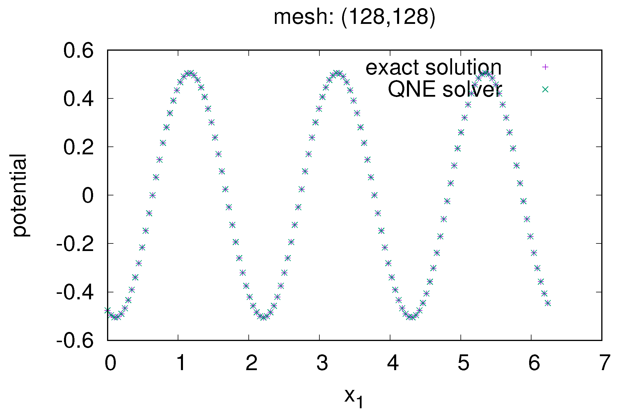
5.1. 1st Example: Double-Periodic Boundary Condition in Cartesian Coordinate

In this example, the periodic boundary condition is used in both $x_1$ and $x_2$ dimensions. According to Equations (A12) and (A13), for the function $f\left(\mathbf{x}\right)=cos(n{x}_1+m{x}_2)$, the exact solution of ${\mathcal{J}}_1\left(\mu \right)f\left(\mathbf{x}\right)$ and ${\mathcal{J}}_2\left(\mu \right){\mathcal{J}}_1\left(\mu \right)f\left(\mathbf{x}\right)$ are

$$\begin{array}{ccc}\hfill {\mathcal{J}}_1\left(\mu \right)cos(n{x}_1+m{x}_2)& =& J_0\left(\rho \left(\mu \right)\sqrt{n^2+m^2}\right)cos(n{x}_1+m{x}_2),\hfill \\ \hfill {\mathcal{J}}_2\left(\mu \right){\mathcal{J}}_1\left(\mu \right)cos(n{x}_1+m{x}_2)& =& J_0^2\left(\rho \left(\mu \right)\sqrt{n^2+m^2}\right)cos(n{x}_1+m{x}_2).\hfill \end{array}$$

Two cases are computed. For the first one, $n=0,m=2$ are used, and $\mu =0.02$, $N_{\theta }=100$, while for the second one, $n=5,m=5$ are chosen. For both cases, we compute the domain $(0,2\pi )\times (0,2\pi )$ which are divided into three meshes of $(16,16),(32,32),(64,64)$ cells, respectively. The results are shown in

Table 1. Double-periodic, Cartesian. $m=2,n=0,\mu =0.02,N_{\theta }=100$.

Mesh	(16,16)	(32,32)	(64,64)
interpo, ${\mathcal{J}}_1$	$1.7084\times {10}^{-2}$	$6.4524\times {10}^{-4}$	$4.1522\times {10}^{-5}$
2nd, ${\mathcal{J}}_1$	0.8738	0.9635	0.9872
interpo, ${\mathcal{J}}_2$	$3.2803\times {10}^{-2}$	$1.2393\times {10}^{-3}$	$7.9757\times {10}^{-5}$
2nd, ${\mathcal{J}}_2$	1.7102	1.8882	1.9352

and

Table 2. Double-periodic, Cartesian. $m=5,n=5,\mu =0.02,N_{\theta }=100$.

Mesh	(16,16)	(32,32)	(64,64)
interpo, ${\mathcal{J}}_1$	1.3114	$4.0744\times {10}^{-2}$	$2.08\times {10}^{-3}$
2nd, ${\mathcal{J}}_1$	10.2513	10.8218	11.0119
interpo, ${\mathcal{J}}_2$	1.3972	$4.5496\times {10}^{-2}$	$2.3258\times {10}^{-3}$
2nd, ${\mathcal{J}}_2$	115.6807	16.7745	17.1429

. It is found that compared with the 2nd-order solver, the interpolation algorithm has better accuracy and its results present the converging rate of the fourth-order accuracy, which is provided by the cubic spline interpolation.

For this double-periodic boundary condition, we also check the convergence of the abs error along with the number of interpolating points on the Larmor circle. We use $m=2,n=2$, the mesh of the rectangular domain is of $32\times 32$ cells, and the magnetic moment equals $0.5$. The results are presented in Figure 2, which shows that the convergence of the numerical abs error versus the number of the interpolating points on the Larmor circle.

5.2. 2nd Example: Natural + Periodic Boundary Condition in Cartesian Coordinate

For this case, the periodic boundary condition is used in $x_2$ dimension, while the natural boundary condition is used in $x_1$ dimension. The function under gyroaverage is $f\left(\mathbf{x}\right)=x_2$. Its first gyroaverage and double gyroaverage are

$${\mathcal{J}}_1\left(f\left(\mathbf{x}\right)\right)=x_2,{\mathcal{J}}_2{\mathcal{J}}_1\left(f\left(\mathbf{x}\right)\right)=x_2.$$

For this case, $\mu =0.05$. The simulated domain $(0,4)\times (0,2\pi )$ are divided into two meshes including $32\times 32$ and $64\times 64$ cells, respectively. The integrals of the absolute value of the error over the simulated domain for the first and double gyroaverage are presented in

Table 3. Natural $+$ periodic, Cartesian. $f\left(\mathbf{x}\right)=x_2,\mu =0.05,N_{\theta }=100$.

Mesh	(32,32)	(64,64)
interpo, ${\mathcal{J}}_1$	$1.0297\times {10}^{-3}$	$1.7507\times {10}^{-2}$
2nd,${\mathcal{J}}_1$	0.0	0.0
interpo, ${\mathcal{J}}_2$	$2.3478\times {10}^{-2}$	$8.3417\times {10}^{-2}$
2nd,${\mathcal{J}}_2$	0.0	0.0

. To obtain this, we ignored the boundary rows in the $x_1$ dimension, for which the natural boundary condition is used. The fact that the abs error of the 2nd-order solver is zero is due to the fact that the first gyroaverage and the double one of $f\left(\mathbf{x}\right)$ depends on the gradient of $f\left(\mathbf{x}\right)$ only through ${\nabla }_{\perp }^{2}f\left(\mathbf{x}\right)$, as Equation (A3) shows. ${\nabla }_{\perp }^{2}f\left(\mathbf{x}\right)$ in Cartesian coordinates is written as $({\partial }_{x_1}^2+{\partial }_{x_2}^2)f\left(\mathbf{x}\right)$. The second order derivative is approximated by the centered finite difference as ${\partial }_{x_1}^{2}f\left(\mathbf{x}\right)=\frac{f_{j+1,k}-2f_{j,k}+f_{j-1,k}}{\delta x_1^2}$ with the 2nd-order precision, where $f_{j+1,k}\equiv f(x_{1,j+1},x_{2,k})$. It is obvious that the finite difference of ${\partial }_{x_1}^2$ over $f\left(\mathbf{x}\right)$ being $x_2$ equals zero, so does ${\partial }_{x_2}^2$ over $f\left(\mathbf{x}\right)$ except at the boundary. The abs error of the 2nd-order solver equaling zero is obtained when the boundary row are ignored.

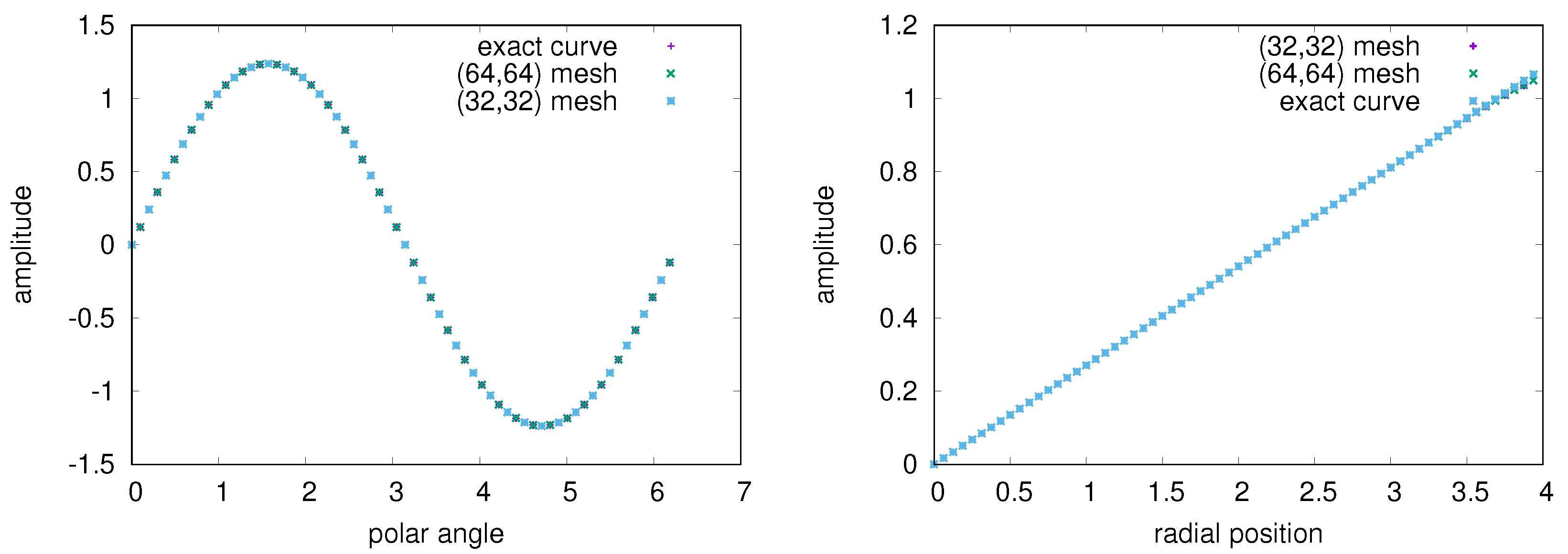
5.3. 3rd Example: Natural + Periodic Boundary Condition in the Polar Coordinate Frame

For this case, the periodic boundary condition is used in $\mathsf{\Theta }$ dimension, while the natural boundary condition used in r dimension. We also use the test function $f\left(\mathbf{x}\right)=x_2$, and the domain is also chosen as $(0,4)\times (0,2\pi )$. The integral of the absolute value of the error is presented in

Table 4. Natural $+$ periodic, polar. $f\left(\mathbf{x}\right)=x_2,\mu =0.02,N_{\theta }=100$.

Mesh	(32,32)	(64,64)
interpo,${\mathcal{J}}_1$	$8.0966\times {10}^{-4}$	$1.0698\times {10}^{-5}$
interpo,${\mathcal{J}}_2$	$1.9712\times {10}^{-2}$	$2.9669\times {10}^{-3}$

. The boundary rows in r dimension are ignored to get these results. The exact profile of the first and double gyroaverage of the test function at the radial position $7/4$ along the polar dimension and the corresponding numerical solutions computed in the two meshes are plotted in the left figure of Figure 3. The exact profile of the first and double gyroaverage of the test function profile at the polar angle $7\pi /8$ along the radial dimension and the corresponding numerical solutions computed in the two meshes are plotted in the right figure of Figure 3. Both figures show that the results computed by the interpolation algorithm fit the exact value very well. However, we can still notice a small error at the outer boundary of $x_1$ dimension, where the natural boundary condition is used.

5.4. Benchmark the QNE Solver in the Cartesian Coordinate Frame and in the Polar Coordinate Frame

The previous examples benchmark the interpolation algorithm to compute the gyroaverage operation. This subsection is dedicated to benchmark the QNE solver, which comprises solving the inverse matrix of $A^{spl}$ and $A_{l,{\rho }_j}^{contri}$ by FFT based on the algorithm given in Section 4.2, and the interpolation algorithm to obtain the gyroaverage.

For the convenience to find the exact solution of QNE, we simplify QNE in Equation (22) by choosing $T_i=T_e=0.5,n_0=n_{g0}=1.0$. We also solve the single $\mu$ case first, so that QNE is simplified as

$$4\varphi \left(\mathbf{x}\right)-{\mathcal{J}}_2\left(\mu \right){\mathcal{J}}_1\left(\mu \right)\varphi \left(\mathbf{x}\right)=n_1\left(\mathbf{x}\right).$$

(43)

We first benchmark the QNE solver in Cartesian coordinate frame with double-periodic boundary condition. By choosing

$$n_1\left(\mathbf{x}\right)=cos(n{x}_1+m{x}_2),$$

the exact solution of Equation (43) is

$$\varphi \left(\mathbf{x}\right)=\frac{cos(n{x}_1+m{x}_2)}{4-J_0^2\left(\rho \left(\mu \right)\sqrt{n^2+m^2}\right)}.$$

We choose $n=3,m=3$, $\mu =1.0$ and $\mu =0$. The simulated domain $(0,4)\times (0,2\pi )$ are divided into three meshes including $32\times 32$, $64\times 64$ and $128\times 128$ cells, respectively. The integrals of the absolute value of the error for the three kinds of mesh are presented in

Table 5. Double-periodic, Cartesian. $n=3,m=3,N_{\theta }=100$.

Mesh	(32,32)	(64,64)	(128,128)
$\mu =1.0$	$1.5204\times {10}^{-4}$	$6.5066\times {10}^{-6}$	$2.9072\times {10}^{-7}$
$\mu =0.0$	$1.2393\times {10}^{-13}$	$1.4944\times {10}^{-13}$	$1.3548\times {10}^{-13}$

, which indicates that the QNE solver could provide a good solution. For the $\mu =0.5$ case, we also plot in Figure 4 the exact solution and the results computed by the QNE solver with node number in $x_2$ dimension equaling 20. The two solutions in Figure 4 fit each other well.

To benchmark the QNE solver in the polar coordinate frame, the function $n_1$ in Equation (43) is chosen as

$$n_1\left(\mathbf{x}\right)=x_2,$$

which leads to the exact solution of $\varphi \left(\mathbf{x}\right)$ through Equation (43)

$$\varphi \left(\mathbf{x}\right)=x_2.$$

The simulated domain $(0,4)\times (0,2\pi )$ is also divided into meshes of $32\times 32$ and $64\times 64$ cells, respectively. We computed two cases of $\mu =0.02$ and $\mu =0$. The integral of the absolute error over the simulated domain for the two $\mu$ cases are given in

Table 6. Natural + periodic, polar. $f\left(\mathbf{x}\right)=x_2,N_{\theta }=100$.

Mesh	(32,32)	(64,64)
$\mu =0.02$	0.1186	0.1339
$\mu =0.0$	$2.6356\times {10}^{-13}$	$1.4944\times {10}^{-13}$

. The fourth-order converging rate does not appear anymore, due to the error at the boundary area where the natural boundary condition is used. The error has two sources. One is that the natural boundary condition is used. The other is that around boundary, due to the finite value of the Larmor radius, there are sampling points located out of the simulated domain and we project these points to the corresponding points at the boundary.

We still plot the exact solution and the numerical solutions of the polar profile at the radial position $7/4$ and the radial profile at the polar angle $7\pi /8$ in Figure 5, which presents good match between the two solutions.

6. Benchmark of the Interpolation Algorithm for the Multiple $\mathit{\mu }$ Case

This benchmark is done in the polar coordinate frame. The test function is chosen as

$$f\left(\mathbf{x}\right)=cos(n{x}_1+m{x}_2).$$

We consider the gyroaverage associated with $\mu$ obeying the distribution $e^{-\mu /a}$ where $a\in (0.5,2.2)$ is chosen.

The integral of the distribution over $\mu$ is written as

$${\mathcal{I}}_0({\mu }_{max},n,m)={\int }_0^{{\mu }_{max}}{e}^{-\mu /a}d\mu$$

and the exact solution of the gyroaverage of the test function $f\left(\mathbf{x}\right)$ are related to the following two functions

$${\mathcal{I}}_1({\mu }_{max},n,m)={\int }_0^{{\mu }_{max}}{J}_0\left(\rho \left(\mu \right)\sqrt{n^2+m^2}\right)e^{-\mu /a}d\mu$$

and

$${\mathcal{I}}_2({\mu }_{max},n,m)={\int }_0^{{\mu }_{max}}{J}_0^2\left(\rho \left(\mu \right)\sqrt{n^2+m^2}\right)e^{-\mu /a}d\mu .$$

The exact solution of the first gyroaverage is

$${\int }_0^{{\mu }_{max}}{\mathcal{J}}_1\left(\mu \right)f\left(\mathbf{x}\right)e^{-\mu /a}d\mu ={\mathcal{I}}_1({\mu }_{max},n,m)f\left(\mathbf{x}\right),$$

and the exact solution of the double gyroaverage is

$${\int }_0^{{\mu }_{max}}{\mathcal{J}}_2\left(\mu \right){\mathcal{J}}_1\left(\mu \right)f\left(\mathbf{x}\right)e^{-\mu /a}d\mu ={\mathcal{I}}_2({\mu }_{max},n,m)f\left(\mathbf{x}\right),$$

which can be written into a discretized formula

$$\sum _{i=1}^{N_{\mu }}{\mathcal{J}}_2\left({\mu }_i\right){\mathcal{J}}_1\left({\mu }_i\right)f\left(\mathbf{x}\right)e^{-{\mu }_i/a}\delta {\mu }_i.$$

6.1. The Euler–Maclaurin-Based Quadrature Integration Algorithm

$\tilde{\mathsf{\Phi }}$ is given in Equation (23) and F is proportional to $exp(-\frac{\mu B}{T_i\left(r\right)})$. To obtain the integral over $\mu$, the conventional way is to redefine a new magnetic moment by ${\mu }_{new}=\mu /T_i\left(r\right)$. Then, the exponential factor $exp(-\frac{\mu B}{T_i\left(r\right)})$ becomes $exp(-{\mu }_{new})$ and the Gauss-Laguerre quadrature is implemented to obtain the discretized sum to approximate the continuous integral. However, in the new term $\tilde{\mathsf{\Phi }}$, the denominate of $T_i\left(r\right)$ in $exp(-\frac{\mu B}{T_i\left(r\right)})$ together with $n_0\left(r\right)$ determines the radial density profile of the ions which possess the magnetic moment $\mu$. As $T_i\left(r\right)$ could possess the steep gradient in the radial dimension, its gyroaverage $\mathcal{J}\left(\mu \right)T_i\left(\mathbf{x}\right)$ cannot be ignored, resulting that $T_i\left(r\right)$ can not be eliminated from the denominate in the conventional way. Moreover, we cannot use Gauss-Laguerre quadrature method to provide the same group of $\mu$ nodes and the associated weights along the radial dimension for different $T_i\left(r\right)$ in the radial domain. Because the value of $T_i\left(r\right)$ is within a domain, which is chosen as $(0.5,2.2)$ in this paper, and the gradient of $T_i\left(r\right)$ after the gyroaverage could also change, the roots and weights provided by Gauss-Laguerre quadrature for the integral ${\int }_0^{{\mu }_{max}}{e}^{-\mu }d\mu$ can not fit the integral ${\int }_0^{{\mu }_{max}}{e}^{-\mu /a}d\mu$ anymore for all as belonging to the domain $(0.5,2.2)$.

We therefore develop a quadrature integrating scheme based on the following Euler–Maclaurin quadrature formula

$$\begin{array}{c}\hfill {\int }_b^{c}f\left(x\right)dx=\frac{h}{2}(f\left(b\right)+f\left(c\right))+\sum _{k=1}^{n-1}hf(b+kh)-\sum _{r=1}^M\frac{h^{2r}{B}_{2r}}{\left(2r\right)!}\left(f^{2r-1}\left(c\right)-f^{2r-1}\left(b\right)\right)+R_p.\end{array}$$

(44)

where $h=(c-b)/n$, $n-1$ is the number of the cells of the mesh, $B_{2r}$ is the $2r$-th Bernoulli number and $R_p$ is the residual quantity. The order of the precision of the right side is beyond $O\left(h^{2M}\right)$. For the distribution function proportional to $exp(-\mu /a)$, $R_p$ and the term depending on $f^{2r-1}\left(c\right)$ can be ignored for large enough c. $B_{2r}$ can be solved by the recurrence relation

$$B_p=-\frac{1}{p+1}\sum _{k=0}^{p-1}\left(\begin{array}{c}p+1\\ k\end{array}\right)B_k.$$

The derivative $f^{2r-1}\left(b\right)$ is replaced by the finite difference scheme. For a function $F\left(x\right)$, the finite difference scheme of the dth order derivative with the pth order precision can be formally written as the following summation of the function value on the grid points

$$\frac{h^d}{d!}{F}^{\left(d\right)}\left(x\right)=\sum _{i=i_{min}}^{i_{max}}{G}_{dpi}F(x+ih)+O\left(h^{d+p}\right),$$

(45)

where $G_{dpi}$ is the coefficient of the finite difference with the pth order precision for the dth order derivative, and the step length of the finite difference is the same with that used in Equation (44). For the forward finite difference scheme of the dth order derivative with pth order precision, $i_{min}=0$ and $i_{max}=d+p-1$ are derived, while for the centered finite difference scheme, we have $-i_{min}=i_{max}=(d+p-1)/2$. By truncating the Taylor expanding of $F(x+ih)$ at the order $O({\left(ih\right)}^{d+p-1})$, Equation (45) can be rewritten as

$$\begin{array}{cc}\hfill F^d\left(x\right)& =\frac{d!}{h^d}\sum _{n=0}^{d+p-1}\left(\sum _{i=i_{min}}^{i_{max}}{i}^n{G}_{dpi}\right)\frac{h^n}{n!}{F}^n\left(x\right)+O\left(h^p\right)\hfill \\ & \approx \frac{d!}{h^d}\sum _{n=0}^{d+p-1}\left(\sum _{i=i_{min}}^{i_{max}}{i}^n{G}_{dpi}\right)\frac{h^n}{n!}{F}^n\left(x\right).\hfill \end{array}$$

(46)

The equaling of both sides of Equation (46) results in the following identities

$$\sum _{i=i_{min}}^{i_{max}}{i}^n{G}_{dpi}=\left\{\begin{array}{c}0,0\le n\le d+p-1\mathrm{and}n\ne d\hfill \\ 1,n=d\hfill \end{array}\right\},$$

through which the coefficient $G_{dpi}$s can be solved. By substituting Equation (46) into the Euler–Maclaurin formula, we obtain its discretized version

$${\int }_b^{c}f\left(x\right)dx=\frac{h}{2}(f\left(b\right)+f\left(c\right))+\sum _{k=1}^{n-1}hf(b+kh)+h\sum _{r=1}^M\frac{B_{2r}}{2r}\sum _{i=i_{min}}^{i_{max}}{G}_{(2r-1)pi}f(b+ih).$$

(47)

For the forward finite difference scheme, Equation (47) can be rearranged into

$$\begin{array}{cc}\hfill {\int }_b^{c}f\left(x\right)dx& =\sum _{i=1}^{2M+p-2}\left[h+h\sum _{\begin{array}{c}1\le r\le M,\\ i\le 2r+p-2\end{array}}\frac{B_{2r}}{2r}{G}_{(2r-1)pi}\right]f(b+ih)\hfill \\ & +\left[\frac{h}{2}+h\sum _{r=1}^M\frac{B_{2r}}{2r}{G}_{(2r-1)p0}\right]f\left(b\right)+\sum _{i=2M+p-1}^{n-1}hf(b+ih)+\frac{h}{2}f\left(c\right),\hfill \end{array}$$

(48)

where we select the condition satisfying $2M+p-1\le n-1$. The weight coefficients of $f(b+ih)$ in Equation (48) for all $i\in \{0,1,2,\cdots ,n-1\}$ are computed and stored at the beginning of the simulation for the following quadrature integration.

For the central difference scheme, Equation (47) can be rearranged in the same way into

$$\begin{array}{cc}\hfill {\int }_b^{c}f\left(x\right)dx& =\sum _{i=1}^{(2M+p-2)/2}\left[hf(b+ih)+h\sum _{\begin{array}{c}1\le r\le M,\\ i\le (2r+p-2)/2\end{array}}\frac{B_{2r}}{2r}\left(G_{(2r-1)pi}f(b+ih)+G_{(2r-1)p(-i)}f(b-ih)\right)\right]\hfill \\ & +\left[\frac{h}{2}+h\sum _{r=1}^M\frac{B_{2r}}{2r}{G}_{(2r-1)p0}\right]f\left(b\right)+\sum _{i=(2M+p)/2}^{n-1}hf(b+ih)+\frac{h}{2}f\left(c\right),\hfill \end{array}$$

(49)

The value of $f(b-ih)$ is obtained by considering the even or odd property of $f(x-b)$ relative to the point $x=b$. The value of b equals 0 for the situation we consider, while the integrand is an even function relative to the point $b=0$.

One more point to mention is that instead of $\mu$, we implement $v_{\perp }$, which equals $\sqrt{2\mu }$, as the integration argument for the achievement of the high precision. So $d\mu =v_{\perp }d{v}_{\perp }$ and the minimal value of $v_{\perp }$ equals 0. Based on this implementation, we developed the third one named derivative-reduction scheme. By replacing $\mu$ with $v_{\perp }$, the integral $\int f\left(2\mu \right)d\mu$ becomes $\int f\left(v_{\perp }^2\right)v_{\perp }d{v}_{\perp }$, with the new integrand being $g\left(v_{\perp }\right)\equiv f\left(v_{\perp }^2\right)v_{\perp }$. At the point $v_{\perp }=0$, we use the following formula to reduce the order of the derivative

$$g^{2k-1}\left(0\right)=(2k-1)f^{2k-2}\left(0\right).$$

Then, the third discretized expression of Euler–Maclaurin formula is derived as

$$\begin{array}{cc}\hfill {\int }_0^{c}g\left(v_{\perp }\right)d{v}_{\perp }& \approx \frac{h}{2}(g\left(0\right)+g\left(c\right))+\sum _{k=1}^{n-1}hg\left(kh\right)+\sum _{r=1}^M\frac{h^{2r}{B}_{2r}}{\left(2r\right)!}{g}^{2r-1}\left(0\right)\hfill \\ & =\frac{h}{2}(g\left(0\right)+g\left(c\right))+\sum _{k=1}^{n-1}hg\left(kh\right)+\sum _{r=1}^M\frac{h^{2r}{B}_{2r}}{\left(2r\right)!}(2r-1)f^{2r-2}\left(0\right)\hfill \\ & =\frac{h}{2}(g\left(0\right)+g\left(c\right))+\sum _{k=1}^{n-1}hg\left(kh\right)+\frac{h^2{B}_2}{2}f\left(0\right)+h^2\sum _{r=2}^M\frac{B_{2r}}{2r}\sum _{i=i_{min}}^{i_{max}}{G}_{(2r-2)pi}f\left(0\right)\hfill \\ & =\frac{h}{2}cf\left(c\right))+\sum _{k=1}^{n-1}h\left(kh\right)f\left(kh\right)+\frac{h^2{B}_2}{2}f\left(0\right)+h^2\sum _{r=1}^M\frac{B_{2r+2}}{2r+2}\sum _{i=i_{min}}^{i_{max}}{G}_{\left(2r\right)pi}f\left(0\right)\hfill \\ & =\sum _{i=1}^{(2M+p-1)/2}\left[h\left(ih\right)f\left(ih\right)+h^2\sum _{\begin{array}{c}1\le r\le M,\\ i\le (2r+p-1)/2\end{array}}\frac{B_{2r+2}}{2r+2}(G_{\left(2r\right)pi}+G_{\left(2r\right)p(-i)})f\left(ih\right)\right]\hfill \\ & +\frac{h^2{B}_2}{2}f\left(0\right)+h^2\sum _{r=1}^M\frac{B_{2r+2}}{2r+2}{G}_{\left(2r\right)p0}f\left(0\right)+\sum _{i=(2M+p-1)/2+1}^{n-1}h\left(ih\right)f\left(ih\right)+\frac{h}{2}cf\left(c\right),\hfill \end{array}$$

(50)

where we have used the even property of the function $f\left(v_{\perp }^2\right)$ at $v_{\perp }=0$, so that $f(-ih)=f\left(ih\right)$.

To test the accuracy and the convergent rate of the three schemes based on the Euler–Maclaurin formula, we apply them to the computation of the exponential integral ${\int }_0^{30}{e}^{-\mu /a}d\mu$ and the associated double-gyroaverage integral ${\int }_0^{30}{J}_0^2\left(\sqrt{2\mu }\right)e^{-\mu /a}d\mu$. In addition, we choose $M=4,p=6$ for the test purpose and for the following other numerical simulation examples. We also compare its results to those computed by the trapezoidal quadrature algorithm with uniform mesh. Through dividing the domain $(0,30)$ into ${10}^7$ equal cells, the two integrals are approximated by the Riemann sum. By treating the Riemann sums as the exact value, the absolute value of the numerical error computed by the two algorithms are plotted in Figure 6 for the three cases $a=0.5,1.0,2.2$. Figure 6 shows that compared with the trapezoidal quadrature algorithm, the three schemes of the Euler–Maclaurin-based algorithm provide a much higher precision order when the nodes number goes from 17 to 129.

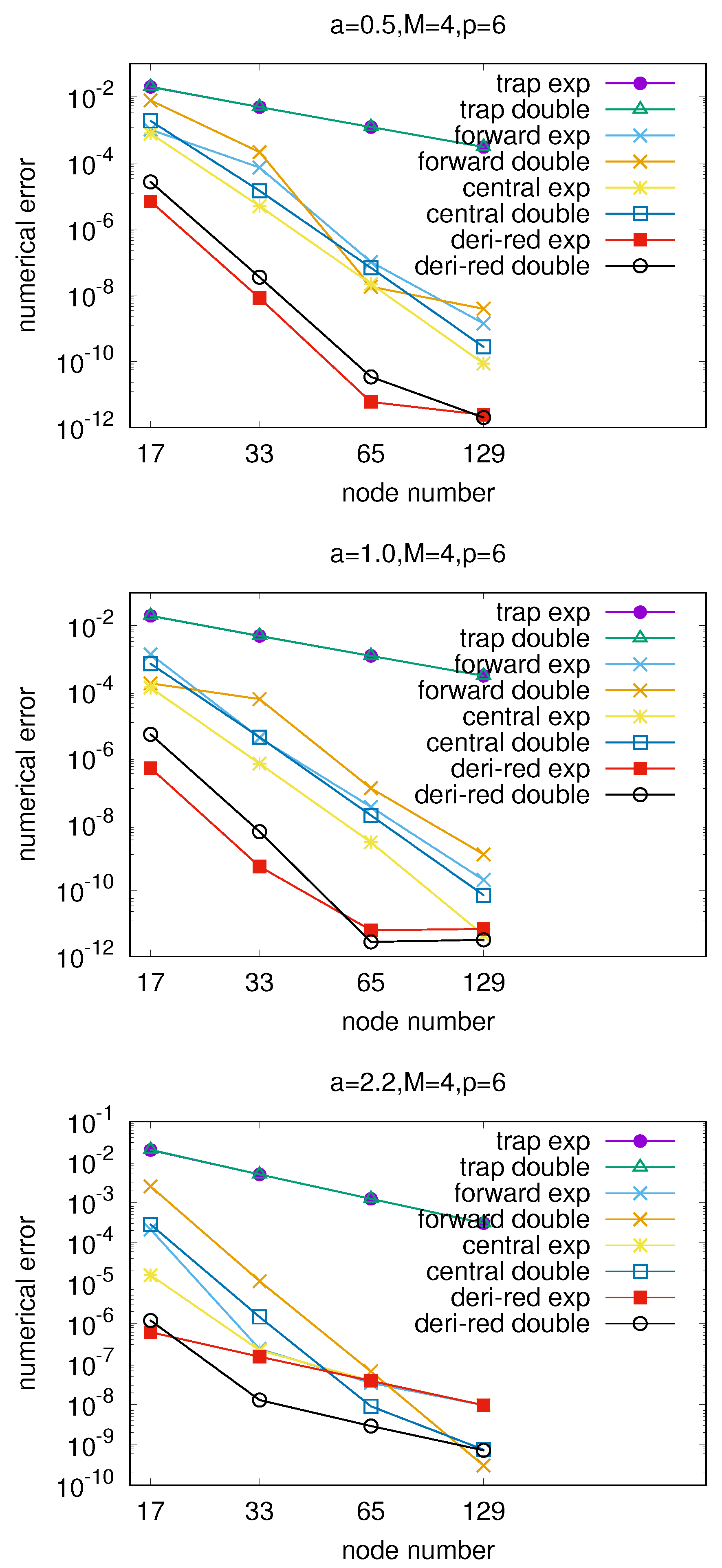
6.2. Benchmark of DGT Computed by the Interpolation Algorithm in the Polar Coordinate Frame Assisted by the Forward Scheme of the Euler–Maclaurin-Based Algorithm

This benchmark is done in the polar coordinate frame and the forward scheme of the Euler–Maclaurin-based algorithm is implemented. In this benchmark, $n=0,m=1$ is chosen. The simulated domain of $(r,\mathsf{\Theta })$ is $(0,16)\times (0,2\pi )$, which is divided into $40\times 40$ meshes. $\mu$ is in $(0,20)$ which is divided into one mesh including 64 nodes. Only the case of $a=1$ is computed here. The polar profile at $r=6$ and the radial profile at $\mathsf{\Theta }=\frac{7\pi }{8}$ are shown in Figure 7.

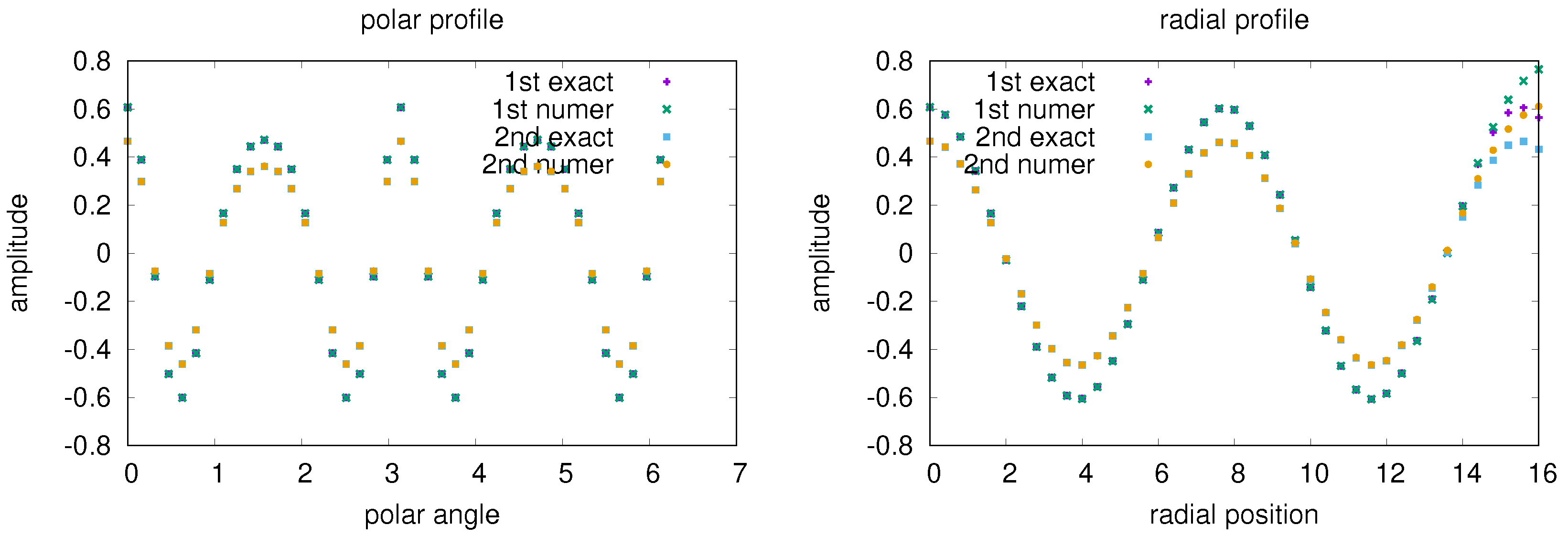
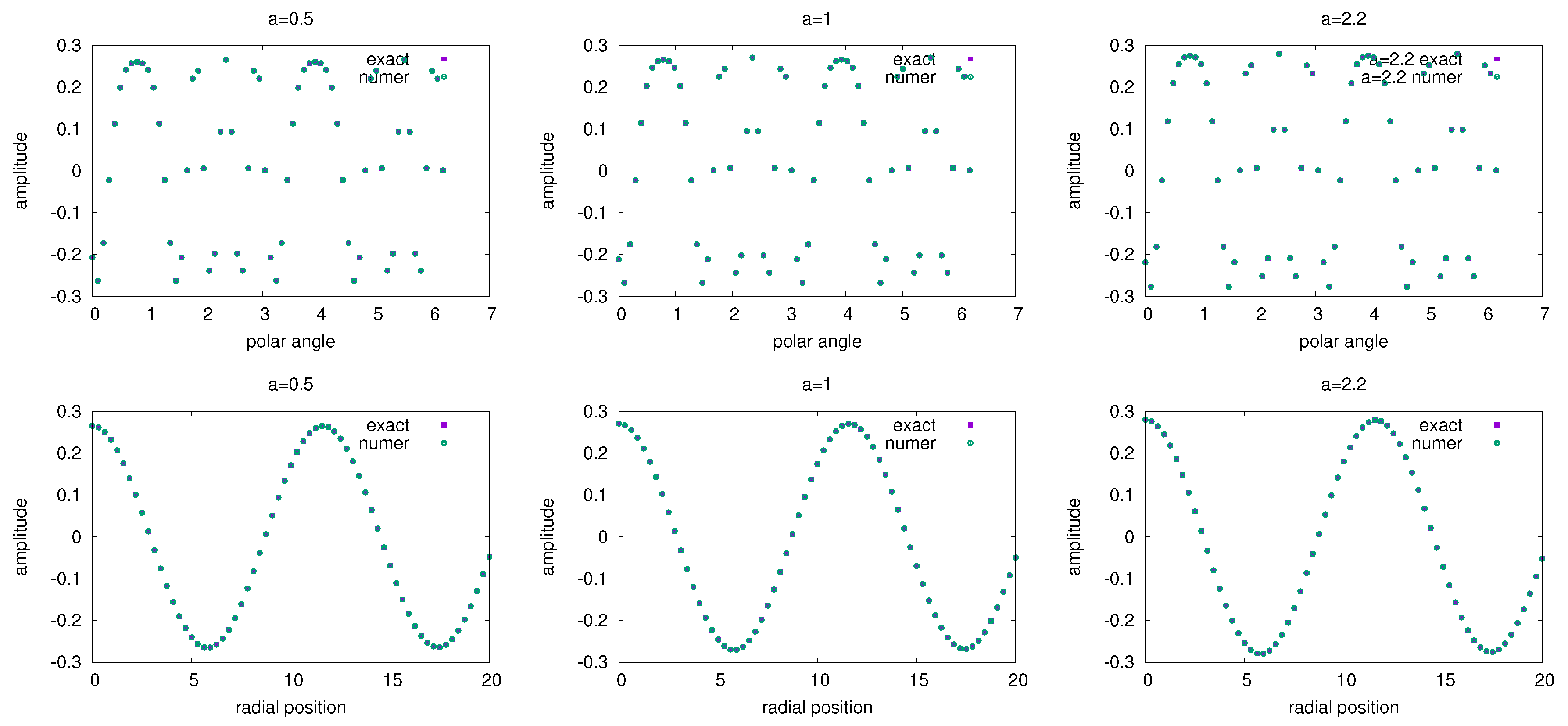
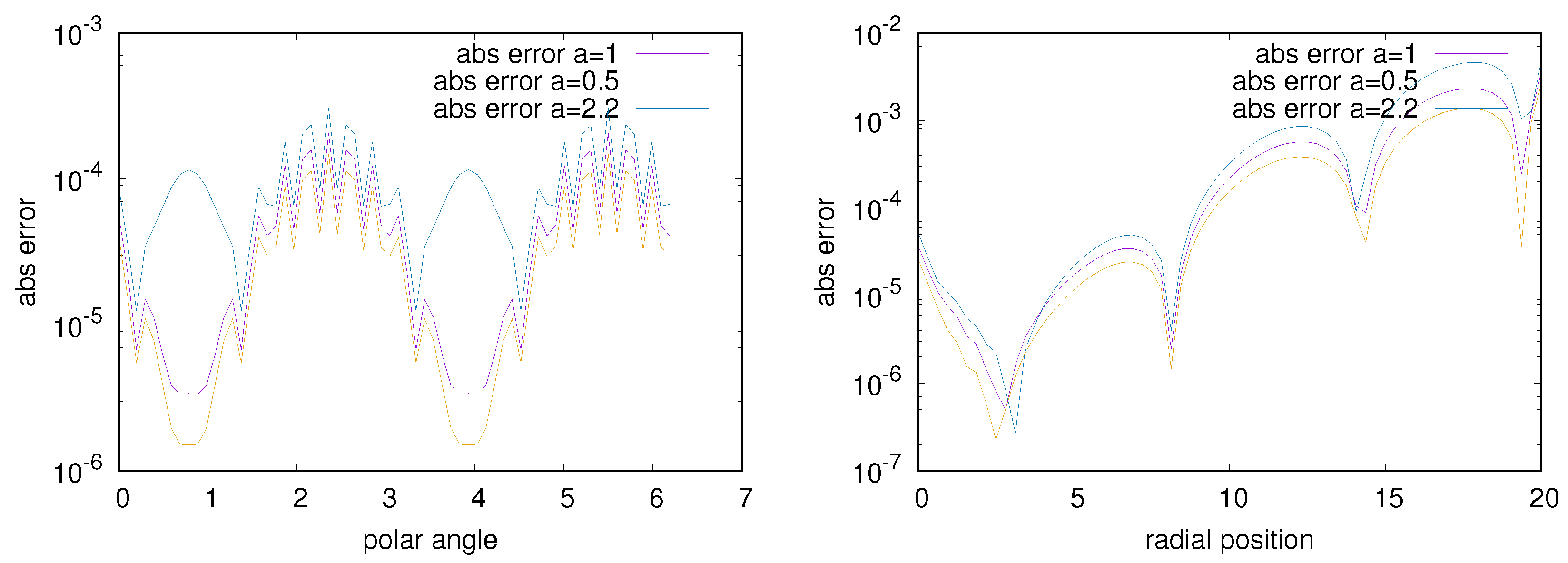
6.3. Benchmark of the QNE Solver in the Polar Coordinate Frame Assisted by the Forward Scheme of the Euler–Maclaurin-Based Algorithm

We also benchmark the QNE solver in the polar coordinate frame with $\mu$ obeying the distribution $e^{-\mu /a}$, with which the quasi-neutrality equation in this case is

$$4\varphi \left(\mathbf{x}\right)-{\int }_0^{{\mu }_{max}}{\mathcal{J}}_2\left(\mu \right){\mathcal{J}}_1\left(\mu \right)\varphi \left(\mathbf{x}\right)e^{-\mu /a}d\mu =n_1\left(\mathbf{x}\right),$$

(51)

where the same parameters $T_{i0},T_{e0},n_0,n_{g0}$ are used. We choose the test function of $n_1\left(\mathbf{x}\right)=cos(n{x}_1+m{x}_2)$. The exact solution of Equation (51) is

$$\varphi \left(\mathbf{x}\right)=\frac{cos(n{x}_1+m{x}_2)}{4-{\mathcal{I}}_2({\mu }_{max},n,m)}.$$

In this benchmark, the radial domain is chosen as $(0,20)$. The domain of $r\times \mathsf{\Theta }$ is divided into a mesh of $64\times 64$ cells. The weights of the $\mu$ mesh for $a=1,0.5,2.2$ are computed by the Euler–Maclaurin-based quadrature algorithm. The magnitude of the numerical error of ${\mathcal{I}}_0$, ${\mathcal{I}}_2$ and the abs error of the integration of the solution over the domain for the three a cases are given in

Table 7. $N_{\mu }=64,n=1,m=1,{\mu }_{max}=20,N_{\theta }=100$.

	$\mathit{a}=1.0$	$\mathit{a}=0.5$	$\mathit{a}=2.2$
${\mathcal{I}}_0$, num error	$2.4991\times {10}^{-5}$	$2.4955\times {10}^{-5}$	$2.662\times {10}^{-5}$
${\mathcal{I}}_2$, num error	$2.4908\times {10}^{-5}$	$2.4925\times {10}^{-5}$	$2.4915\times {10}^{-5}$
solution abs error	1.3817	0.653	3.6886

. The computing formula of the abs error is presented by Equation (42). In Figure 8, the radial profile at $\mathsf{\Theta }=\frac{7\pi }{8}$ and the polar profile at $r=\frac{35}{4}$ for $a=0.5$, $a=1$, $a=2.2$ cases are plotted. The absolute value of the numerical error of the polar profile and the radial profile are plotted in the left and right figure of Figure 9.

7. Application of the QNE Solver in Gyrokinetic Simulation Concerning Short-Scale Perturbation and Steep Equilibrium Profile Assisted by the Forward Scheme of the Euler–Maclaurin-Based algorithm

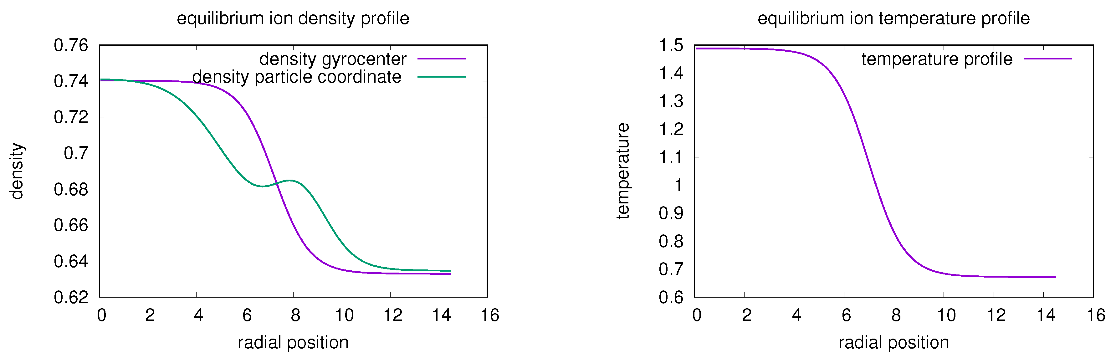
7.1. The Gyrokinetic Model with Constant Cylindrical Magnetic Field Configuration

The cylindrical coordinates frame with the constant theta-pinch magnetic field configuration is used in our simulations. For this configuration adapted in this paper, the equilibrium magnetic field is along the z direction and its magnitude is constant in the cross surface. The periodic boundary condition is used in the parallel dimension and in the polar dimension, while the natural boundary condition in the radial dimension. The whole simulations are executed on the ATLAS HPC platform of IRMA by introducing our test modules into SeLaLiB code [32], which is a classic semi-Lagrangian library using cubic splines interpolation [33,34,35,36]. The predictor-corrector method, the Verlet algorithm for computing the characteristics, and the Strang splitting of the advection of Vlasov equation are also implemented [35,37,38,39,40].

The gyrokinetic Vlasov equation in cylindrical coordinate frame is

$$\left[{\partial }_t+(\frac{1}{r}{\partial }_{\mathsf{\Theta }}\mathsf{\Phi }{\partial }_r-\frac{1}{r}{\partial }_r\mathsf{\Phi }{\partial }_{\mathsf{\Theta }})+U{\partial }_{x_{\parallel }}+{\partial }_{x_{\parallel }}\mathsf{\Phi }{\partial }_U\right]F=0.$$

(52)

The characteristics are

$$\begin{array}{ccc}\hfill \dot{r}& =& \frac{1}{r}{\partial }_{\mathsf{\Theta }}\mathsf{\Phi },\hfill \end{array}$$

(53a)

$$\begin{array}{ccc}\hfill \dot{\mathsf{\Theta }}& =& -\frac{1}{r}{\partial }_r\mathsf{\Phi },\hfill \end{array}$$

(53b)

$$\begin{array}{ccc}\hfill \dot{x_{\parallel }}& =& U,\hfill \end{array}$$

(53c)

$$\begin{array}{ccc}\hfill \dot{U}& =& {\partial }_{x_{\parallel }}\mathsf{\Phi }\hfill \end{array}$$

(53d)

The quasi-neutrality equation is given by Equation (22).

7.2. The Parallelization

7.2.1. The Algorithm to Reduce the Distribution to the Density

In the discrete version of $\mu$, the distribution of ions associated with each ${\mu }_j$ with $j\in \{1,\cdots ,N_{\mu }\}$ is denoted as $F_j(\mathbf{x},{\mu }_j,U)$. Due to the identity $\frac{d{\mu }_j}{dt}=0$, $F_j(\mathbf{x},{\mu }_j,U)$ satisfies the Vlasov equation in the cylindrical coordinate system

$$\left[{\partial }_t+(\frac{1}{r}{\partial }_{\mathsf{\Theta }}\mathsf{\Phi }(\mathbf{x},{\mu }_j){\partial }_r-\frac{1}{r}{\partial }_r\mathsf{\Phi }(\mathbf{x},{\mu }_j){\partial }_{\mathsf{\Theta }})+U{\partial }_{x_{\parallel }}+{\partial }_{x_{\parallel }}\mathsf{\Phi }(\mathbf{x},{\mu }_j){\partial }_U\right]F_j(\mathbf{x},{\mu }_j,U)=0,$$

(54)

where $(r,\mathsf{\Theta },x_{\parallel })$ denotes the cylindrical coordinate frame. $F_j(\mathbf{x},{\mu }_j,U)$ can be rewritten as the sum

$$F_j(\mathbf{x},{\mu }_j,U)=F_{0j}(\mathbf{x},{\mu }_j,U)+F_{1j}(\mathbf{x},{\mu }_j,U),$$

with

$$F_{0j}(\mathbf{x},{\mu }_j,U)=F_{0j\parallel }(\mathbf{x},U)F_{0j\perp }(\mathbf{x},{\mu }_j)$$

(55)

and $F_{0j\perp }(\mathbf{x},{\mu }_j)=\frac{1}{2\pi T_i}exp(-\frac{{\mu }_{j}B\left(\mathbf{x}\right)}{T_i\left(\mathbf{x}\right)})$. In the numerical simulation, $F_{0j}(\mathbf{x},{\mu }_j,U)$ does not evolve. At each time step, $F_j(\mathbf{x},{\mu }_j,U)$ is obtained by solving Equation (54) and $F_{1j}(C,{\mu }_j,U)$ is derived by using $F_j(\mathbf{x},{\mu }_j,U)$ minus $F_{0j}(\mathbf{x},{\mu }_j,U)$.

The normalized version of Equations (17a) and (17b) to obtain $n_{sg0}$ and $n_{sg1}$ can be discretized in the $\mu$ dimension by obtaining a mesh of $\mu$ with $N_{\mu }$ nodes. The contribution of each ${\mu }_j$ component to the density $n_{sg}$ and $n_{sg0}$ can be written as

$$\begin{array}{ccc}\hfill n_{sgj}\left(\mathbf{x}\right)& =& B\left(\mathbf{x}\right)\delta {\mu }_j\int F_s\left(\mathbf{x}-{\mathbf{\rho }}_0(\mathbf{x},{\mu }_j),{\mu }_j,U\right)dU,\hfill \\ \hfill n_{sg0j}\left(\mathbf{x},t\right)& =& B\left(\mathbf{x}\right)\delta {\mu }_j\int F_{s0}\left(\mathbf{x}-{\mathbf{\rho }}_0(\mathbf{x},{\mu }_j),{\mu }_j,U\right)dU.\hfill \end{array}$$

Then, the $n_{sg1j}$ can be derived as $n_{sgj}-n_{sg0j}$. In addition, the summation of all ${\mu }_j$s leads to the total density. The specific procedures to compute the density on the particle coordinate frame are listed below:

• The distribution $F_j(\mathbf{x},{\mu }_j,U,t)$ for each ${\mu }_j$ at time moment t is computed by Equation (54).
• The integration of the distribution of each $F_j(\mathbf{x},{\mu }_j,U,t)$ over U is first done by the sum ${\mathcal{S}}_j(\mathbf{x},t)\equiv \sum _j{F}_j(\mathbf{x},{\mu }_j,U_k,t)\delta U$.
• The gyroaverage of ${\mathcal{S}}_j(\mathbf{x},t)$ denoted as ${\mathcal{J}}_2\left({\mu }_j\right){\mathcal{S}}_j(\mathbf{x},t)$ for each ${\mu }_j$ is done by using the coefficient matrix with the result being $A_{2,{\rho }_j}^{contr}{A}^{spl}{\mathcal{S}}_{jt}$, where ${\mathcal{S}}_{jt}$ is a vector formed by ${\mathcal{S}}_j(\mathbf{x},t)$ on the grids and is given as

  $${\mathcal{S}}_{jt}:={({\mathcal{S}}_{j,0,0},\cdots ,{\mathcal{S}}_{j,N_r,0},{\mathcal{S}}_{j,0,1},\cdots ,{\mathcal{S}}_{j,N_r,1},\cdots ,{\mathcal{S}}_{j,0,N_{\mathsf{\Theta }-1}},\cdots ,{\mathcal{S}}_{j,N_r,N_{\mathsf{\Theta }-1}})}^T$$
  The total density on the particle coordinate mesh contributed by the ${\mu }_j$ component is written as

  $$n_{gj,hp}\equiv {\left({\mathcal{J}}_2\left({\mu }_j\right){\mathcal{S}}_j\right)}_{hp},h\in \{0,\cdots ,N_r\},p\in \{0,\cdots ,N_{\mathsf{\Theta }}-1\}.$$
• The equilibrium density in the particle coordinate frame obtained from the gyroaverage of the equilibrium distribution $F_{0j}(\mathbf{x},{\mu }_j,U)$ for the ${\mu }_j$ component is done at the beginning following the procedure $2,3$ and is stored for the subsequent invoking. By inheriting the symbol used in Equation (A6), the jth equilibrium density on particle coordinate spatial mesh is denoted as $n_{g0j,hp}$. Then, the perturbative density on the particle coordinate spatial mesh contributed by the ${\mu }_j$ component is

  $$n_{g1j,hp}=n_{gj,hp}-n_{g0j,hp}.$$

  (56)
• The total perturbative density on the particle coordinate space computed by all $j\in \{1,\cdots ,N_{\mu }\}$ is obtained by “MPI_ALLREDUCE” the $n_{g1j,hp}$ as $\sum _j{n}_{g1j,hp}{B}_{hp}\delta {\mu }_j$, where $B_{hp}$ is the magnetic field magnitude at the node denoted by $(h,p)$.

For an initial equilibrium density profile on the gyrocenter coordinate frame shown by the purple line of Figure 1, assuming the equilibrium distribution of $\mu$ obeying Equation (58), the density on the particle coordinate space after the gyroaverage operation is obtained and shown in Figure 1.

7.2.2. The Parallelization

MPI is used to the parallelization of the computing of $\mu$. The processors are divided into $N_{\mu }$ sub-communicators. $F_j(\mathbf{x},{\mu }_j,U)$ with $j\in \{1,\cdots ,N_{\mu }\}$ is exclusively computed by the jth sub-communicator. In addition, the respective precomputing matrixes of ${\mathsf{\Phi }}_j$ are stored in the jth sub-communicator. $\tilde{\mathsf{\Phi }}$ and $n_{i1}\left(\mathbf{x}\right)$ in Equations (23) and (17b) are computed by “MPI_ALLREDUCE” the respective quantity stored in the processors of the same “color” with respect to the respective sub-communicator.

To calculate the advection of distribution function in the 4D domain $(r,\mathsf{\Theta },x_{\parallel },U)$, two parallelization schemes are involved: the one for parallelizing $x_{\parallel }$ with $r,\mathsf{\Theta },U$ sequential is used to calculate the advection due to $\dot{r},\dot{\mathsf{\Theta }},\dot{U}$; the other one for parallelizing $r,\mathsf{\Theta },U$ with $x_{\parallel }$ sequential is used to compute the advection due to U. The 3D domain $(r,\mathsf{\Theta },x_{\parallel })$ with respect to the potential function and the density implements the scheme: the parallelization in $x_{\parallel }$ with $r,\mathsf{\Theta }$ sequential is used to compute the characteristics $\dot{r},\dot{\mathsf{\Theta }},\dot{U}$ which are needed in computing the advection of the distribution in $r,\mathsf{\Theta },U$ dimensions, and to solve QNE in the poloidal cross-section.

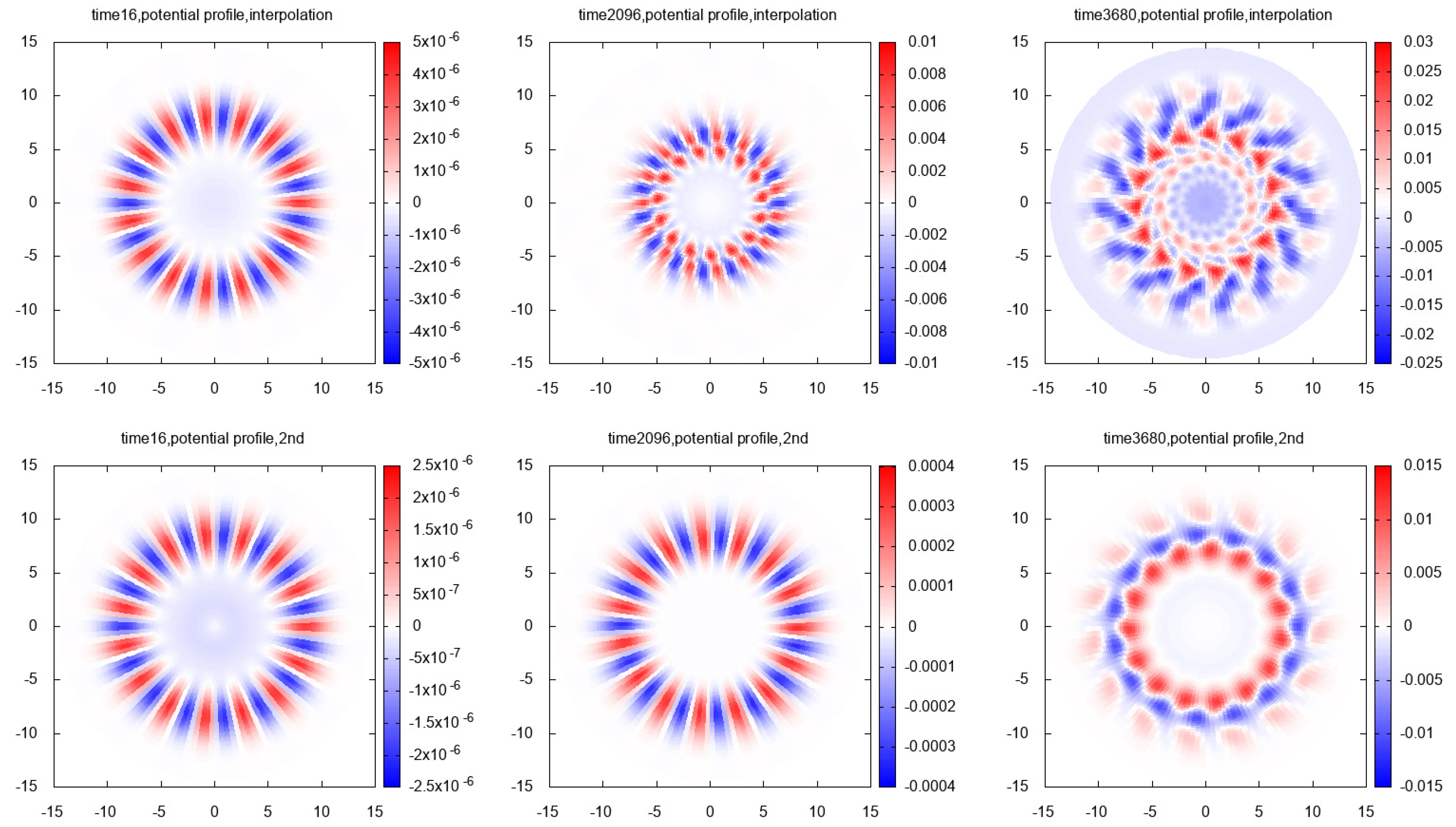
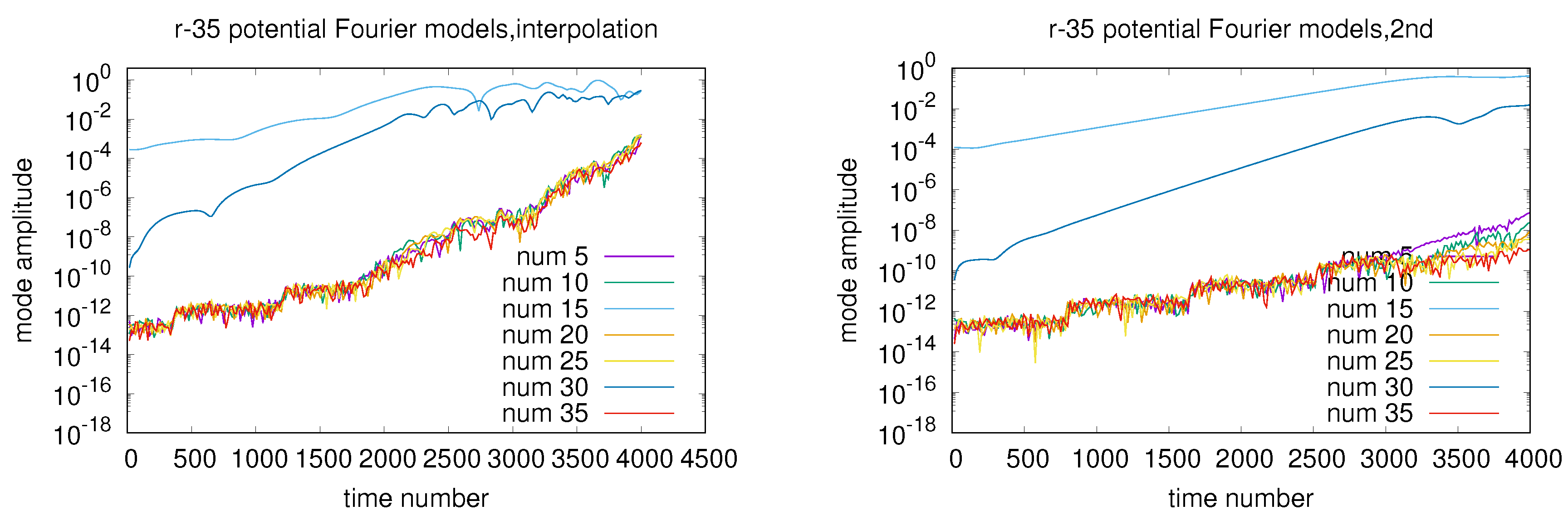
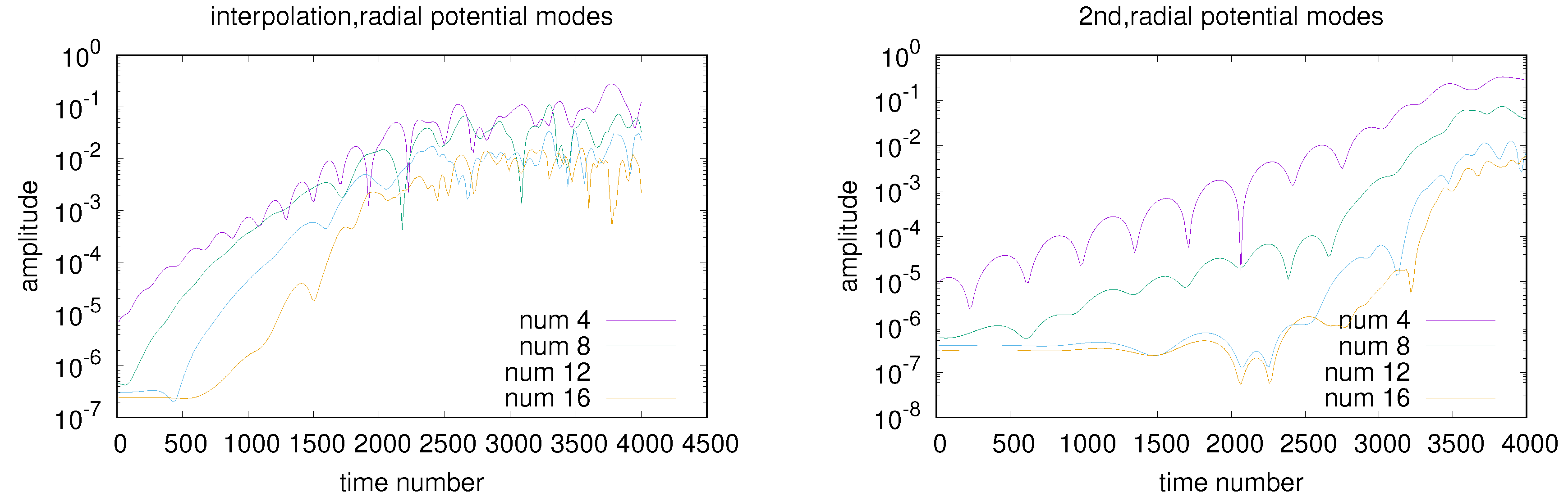
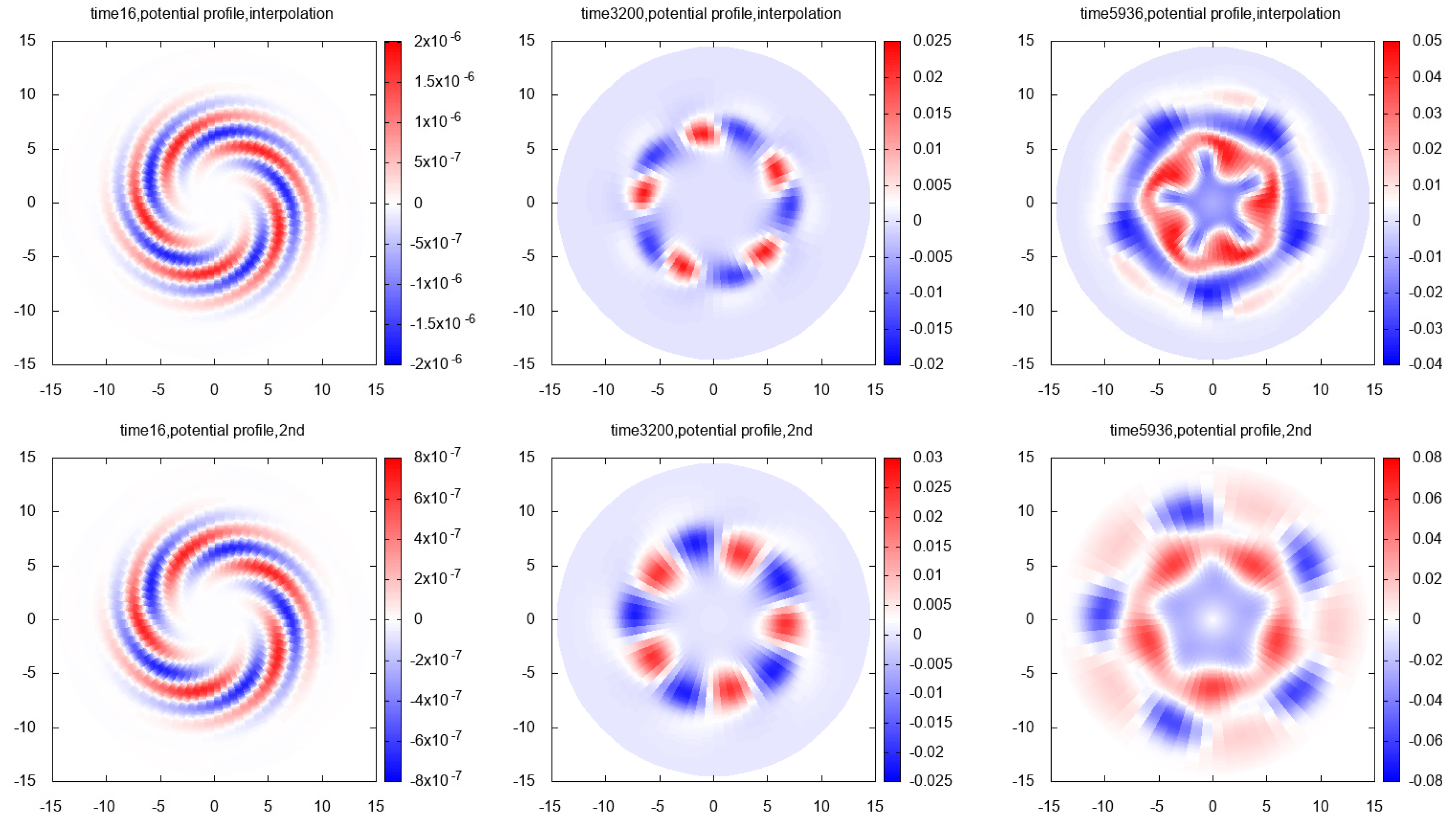
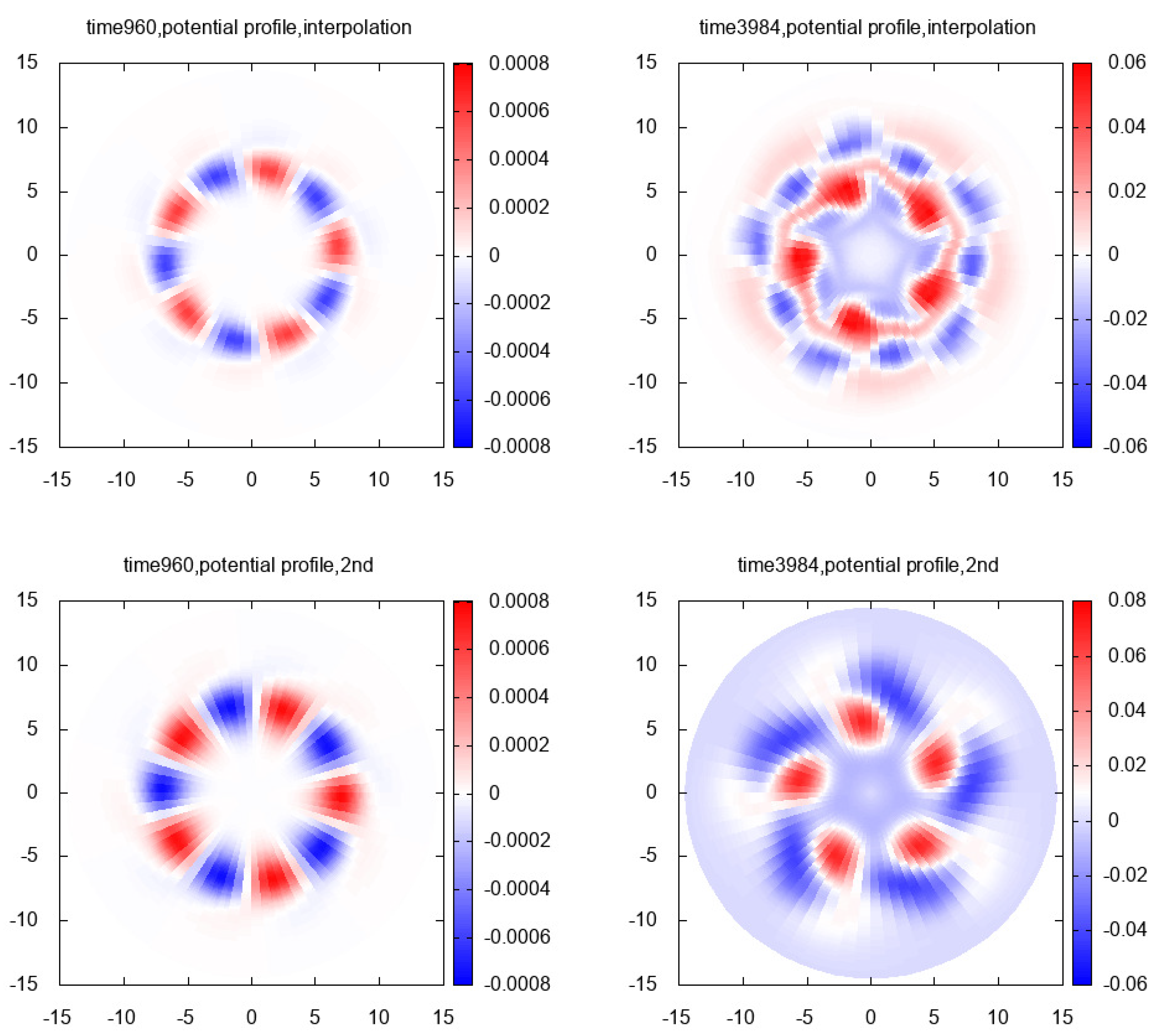
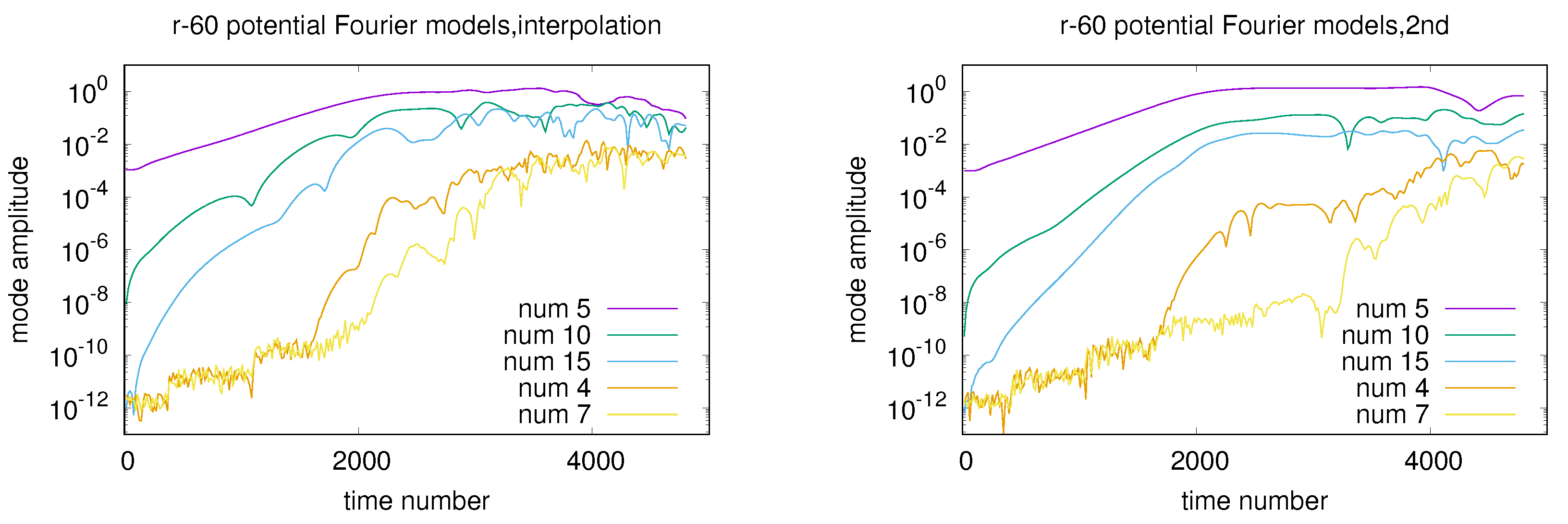
7.3. The Simulation Results

In the cylindrical coordinates system, the initial distribution is of the structure in Equation (14). The distribution function is specifically given as

$$F(0,r,\mathsf{\Theta },x_{\parallel })=F_{eq}\left(r,\mu ,U\right)\times \left(1+\eta exp\left(-\frac{{(r-r_p)}^2}{\delta r}\right)\sum _{n_p,m_p}cos(\frac{2\pi n_p}{L_{\parallel }}{x}_{\parallel }+m_p\mathsf{\Theta }+\frac{2\pi p_p}{L_r}r)\right),$$

(57)

where the equilibrium function $F_{eq}$ is

$$F_{eq}\left(r,\mu ,U\right)=\frac{n_0\left(r\right)exp\left(-\frac{U^2}{2T_i\left(r\right)}-\frac{\mu B}{T_i\left(r\right)}\right)}{{\left(2\pi T_i\left(r\right)\right)}^{3/2}},$$

(58)

where $\eta$ is the parameter for the amplitude of the perturbation, and $n_p,m_p,p_p$ are the respective mode numbers. The profile $T_i\left(r\right)$, $T_e\left(r\right)$ and $n_0\left(r\right)$ are given by:

$$\mathcal{P}\left(r\right)=C_{\mathcal{P}}exp\left(-{\kappa }_{\mathcal{P}}\delta r_{\mathcal{P}}tanh\left(\frac{r-r_{\mathcal{P}}}{\delta r_{\mathcal{P}}}\right)\right)$$

(59)

where $\mathcal{P}\in \{T_i,T_e,n_0\}$, $C_{T_i}=C_{T_e}=1$, and

$$C_{n_0}=\frac{r_{max}-r_{min}}{{\int }_{r_{min}}^{r_{max}}exp\left(-{\kappa }_{n_0}\delta r_{n_0}tanh\left(\frac{r-r_p}{\delta r_{n_0}}\right)\right)dr}.$$

(60)

In Equation (59), ${\mathcal{C}}_{\mathcal{P}}$ is the normalized factor; the magnitude of ${\kappa }_{\mathcal{P}}$ mainly determines the wide between ${\mathcal{P}}_{max}$ and ${\mathcal{P}}_{min}$; the magnitude of $\delta r_{\mathcal{P}}$ determines mainly the steep of the gradient of the profile of $\mathcal{P}$.

For all the following simulation cases, the time step $\Delta t=8$ is chosen and the data are stored every two time steps.

7.3.1. 1st Case: $n_p=1,m_p=0,p_p=0$

This case implements the perturbation not including the polar and radial modes. The used equilibrium profiles of ions’ density and temperature are not steep in the radial dimension and are given in Figure 10. We consider the parameters: $\eta ={10}^{-4}$, ${\kappa }_{n_0}=13.0$, ${\kappa }_{T_i}={\kappa }_{T_e}=20.0$, $\delta r_{n_0}=2.0$, $\delta r_{T_i}=\delta r_{T_e}=1.0$, $L_{\parallel }=1506.759067$, $r_p=0.45(r_{min}+r_{max})$, $\delta r=\frac{4\delta r_{n_0}}{\delta r_{T_i}}$.

The simulated domain of $r\times \mathsf{\Theta }\times x_{\parallel }\times U\times \mu$ is chosen as $(0.5\Delta r,14.5)\times [0,2\pi )\times (0,1506.759067)\times (-7.32,7.32)\times (0,20)$, where $\Delta r$ is the length step in radial direction. This domain is divided into a mesh of $64\times 64\times 32\times 32\times 63$ cells. The simulation is carried out by implementing 128 processes, which are executed by 4 nodes on ATLAS HPC of IRMA using hyperthreading. Each node has 24 CPUs and carries on 32 processes.

The evolution curves of the polar modes of the potential at the radial node 30 are shown in Figure 11. The radial spectrum evolution is shown in Figure 12. A good match of the results computed by the two solvers is revealed by these figures.

7.3.2. 2nd Case: $n_p=1,m_p=15,p_p=0$

For this case, we could obtain $k_{\mathsf{\Theta }}\rho \approx 2$ at $r=7$ with $\rho =1$. We consider the parameters: $\eta ={10}^{-4}$, ${\kappa }_{n_0}=13.0$, ${\kappa }_{T_i}={\kappa }_{T_e}=66.0$, $\delta r_{T_e}=\delta r_{T_e}=\delta r_{n_0}=0.2$, $L_{\parallel }=1506.759067$, $r_p=0.45(r_{min}+r_{max})$, $\delta r=\frac{4\delta r_{n_0}}{\delta r_{T_i}}$. The equilibrium profile of ion’s density and temperature are given by Figure 13.

The simulated domain is the same with that of the 1st case and is divided into a mesh of $64\times 128\times 32\times 32\times 63$ cells. For this case, the implementation of the processes and the partition of these processes on the nodes of ATLAS are the same with that of the 1st case.

The potential profile on the polar cross-section at time moment $16,2096,3680$ computed by the two solvers are shown in Figure 14. The ion temperature modes are driven by the equilibrium gradient. The evolution curves of the polar modes of the potential at the radial node 35 are presented in Figure 15, which shows that the growth rate computed by the interpolation algorithm is larger and the saturation time is earlier. The radial spectrum evolution is shown in Figure 16.

7.3.3. 3rd Case: $n_p=1,m_p=5,p_p=7$

For this case, we could obtain $k_r\rho \approx \pi$ with $\rho =1$. We consider the parameters: $\eta ={10}^{-4}$, ${\kappa }_{n_0}=13.0$, ${\kappa }_{T_i}={\kappa }_{T_e}=66.0$, $\delta r_{T_e}=\delta r_{T_e}=\delta r_{n_0}=0.1$, $L_{\parallel }=1506.759067$, $r_p=0.45(r_{min}+r_{max})$, $\delta r=\frac{4\delta r_{n_0}}{\delta r_{T_i}}$. The equilibrium profile of ion’s density and temperature are given by Figure 17.

The simulated domain is the same and is divided into a mesh of $128\times 64\times 32\times 32\times 63$ cells. The implementation of the processes on the nodes of ATLAS does not change. The potential profile on the polar cross-section at time moment $16,3200,5236$ computed by the two solvers are shown in Figure 18. The evolution curves of the polar modes of the potential at the radial node 35 are presented in Figure 19. The radial spectrum evolution is given in Figure 20.

7.3.4. 4th Case: $n_p=1,m_p=5,p_p=0$

The parameters of this case are the same with those used in the 3rd case except that $p_p=0$ is chosen. The results are plotted in Figure 21, Figure 22 and Figure 23. Compared with the simulation results of the 3rd case, it can be observed from both figures that the growth rate of the polar Fourier modes without the initial radial wavelength are much larger than that with the presence of the initial radial wavelength. Such a fact may contribute a new element to the turbulence induced transport theory, which states that the shear flow could reduce the radial coherent length of the turbulent vortex, mitigating the transport rate as a consequence. Our simulations in 3rd and 4th cases suggest that with the presence of the low toroidal mode number, the short radial wavelength causes much smaller growth rate of the poloidal modes.

8. Conclusions and Discussion

This paper points out that the traditional low-order approximation of DGT is not suitable concerning the short-scale perturbation and the steep equilibrium profile. To obtain the more precise mesh-grids value of the function which is under the first gyroaverage or double gyroaverage in the presence of these extreme cases, the interpolation algorithm is developed by uniformly laying out many points on the Larmor circle surrounding the grid point, the function value at which is obtained by using the cubic spline piecewise basis function for the interpolation. Due to the periodic boundary condition of the cubic spline interpolation on the polar dimension, the interpolation coefficient matrix has the periodic block structure. Then, FFT can be implemented to speed up the process of obtaining the inverse of the discretized coefficient matrix of QNE. Since the density of each ${\mu }_j$ depends on a weight factor $exp(\frac{-\mu B\left(\mathbf{x}\right)}{T_e\left(\mathbf{x}\right)})$ and all quantities as the functions of $\mathbf{x}$ experience a transform $\mathbf{x}\to \mathbf{x}-{\mathit{\rho }}_0(\mathbf{x},{\mu }_j,\theta )$, the Gaussian-Laguerre quadrature integrating method cannot be used and we developed an Euler–Maclaurin-based quadrature integrating method to obtain the quadrature integration for the distribution of $\mu$.

The interpolation algorithm itself and the interpolation solver for the numerical computation of QNE are benchmarked under various boundary conditions based on various analytical solutions. it is found that numerical solutions computed by both cases match the analytical solutions very well. The interpolation solver is also applied to the gyrokinetic integrated simulation which comprises the other Vlasov solver and the characteristic solver. The perturbations possessing various model numbers and the equilibrium profiles possessing various radial gradient are implemented in the integrated simulations. To observe the advantage of the interpolation algorithm, its numerical results are compared with those computed by the 2nd-order solver. When the equilibrium profile is not steep and the perturbation only has the non-zero mode number along the parallel spatial dimension, the results computed by the interpolation solver and the 2nd-order solver match each other well. When the gradient of the equilibrium profile is steep, the interpolation solver provides a bigger driving effect for the ion-temperature-gradient modes which possesses large polar mode numbers.

References

- Diamond, P.H.; Itoh, S.I.; Itoh, K.; Hahm, T.S. Zonal flows in plasma—A review. Plasma Phys. Control. Fusion 2005, 47, R35. [Google Scholar] [CrossRef]
- Lin, Z.; Hahm, T.S.; Lee, W.W.; Tang, W.M.; White, R.B. Turbulent Transport Reduction by Zonal Flows: Massively Parallel Simulations. Science 1998, 281, 1835–1837. [Google Scholar] [CrossRef] [PubMed] [Green Version]
- Biglari, H.; Diamond, P.H.; Terry, P.W. Influence of sheared poloidal rotation on edge turbulence. Phys. Fluids B Plasma Phys. 1990, 2, 1. [Google Scholar] [CrossRef]
- Wesson, J. Tokamaks, 3rd ed.; CLARENDON Press: Oxford, UK, 2004. [Google Scholar]
- Chen, F. Introduction to Plasma Physics and Controlled Fusion; Springer: New York, NY, USA, 2010. [Google Scholar]
- Hazeltine, R.D.; Meiss, J.D. Plasma Confinement; Addison-Wesley, Advanced Book Program: Boston, MA, USA, 1992. [Google Scholar]
- White, R.B. Theory of Tokamak Plasmas, 1st ed.; Elsevier: Amsterdam, The Netherlands, 1989. [Google Scholar]
- Zohm, H. Edge localized modes (ELMs). Plasma Phys. Control. Fusion 1996, 38, 105. [Google Scholar] [CrossRef]
- Hayashi, N.; Takizuka, T.; Aiba, N.; Oyama, N.; Ozeki, T.; Wiesen, S.; Parail, V. Integrated simulation of ELM energy loss and cycle in improved H-mode plasmas. Nucl. Fusion 2009, 49, 95015. [Google Scholar] [CrossRef]
- Burrell, K.H.; West, W.P.; Doyle, E.J.; Austin, M.E.; Casper, T.A.; Gohil, P.; Greenfield, C.M.; Groebner, R.J.; Hyatt, A.W.; Jayakumar, R.J.; et al. Advances in understanding quiescent H-mode plasmas in DIII-D. Phys. Plasmas 2005, 12, 56121. [Google Scholar] [CrossRef]
- Hubbard, A.E. Physics and scaling of the H-mode pedestal. Plasma Phys. Control. Fusion 2000, 42, A15. [Google Scholar] [CrossRef]
- Lönnroth, J.S.; Parail, V.; Dnestrovskij, A.; Figarella, C.; Garbet, X.; Wilson, H.; Contributors, J.E. Predictive transport modelling of type I ELMy H-mode dynamics using a theory-motivated combined ballooning–peeling model. Plasma Phys. Control. Fusion 2004, 46, 1197. [Google Scholar] [CrossRef]
- Ryter, F.; Angioni, C.; Beurskens, M.; Cirant, S.; Hoang, G.T.; Hogeweij, G.M.D.; Imbeaux, F.; Jacchia, A.; Mantica, P.; et al. Experimental studies of electron transport. Plasma Phys. Control. Fusion 2001, 43, A323. [Google Scholar] [CrossRef]
- Suttrop, W. The physics of large and small edge localized modes. Plasma Phys. Control. Fusion 2000, 42, A1. [Google Scholar] [CrossRef]
- Dickinson, D.; Saarelma, S.; Scannell, R.; Kirk, A.; Roach, C.M.; Wilson, H.R. Towards the construction of a model to describe the inter-ELM evolution of the pedestal on MAST. Plasma Phys. Control. Fusion 2011, 53, 115010. [Google Scholar] [CrossRef]
- Garbet, X.; Idomura, Y.; Villard, L.; Watanabe, T.H. Gyrokinetic simulations of turbulent transport. Nucl. Fusion 2010, 50, 43002. [Google Scholar] [CrossRef]
- Lee, W.W. Gyrokinetic particle simulation model. J. Comput. Phys. 1987, 72, 243. [Google Scholar] [CrossRef]
- Lee, W.W. Gyrokinetic approach in particle simulation. Phys. Fluids 1983, 26, 556–562. [Google Scholar] [CrossRef]
- Dubin, D.H.E.; Krommes, J.A.; Oberman, C.; Lee, W.W. Nonlinear gyrokinetic equations. Phys. Fluids 1983, 26, 3524–3535. [Google Scholar] [CrossRef]
- Lin, Z.; Tang, W.M.; Lee, W.W. Gyrokinetic particle simulation of neoclassical transport. Phys. Plasmas 1995, 2, 2975–2988. [Google Scholar] [CrossRef]
- Wang, W.X.; Lin, Z.; Tang, W.M.; Lee, W.W.; Ethier, S.; Lewandowski, J.L.V.; Rewoldt, G.; Hahm, T.S.; Manickam, J. Gyro-kinetic simulation of global turbulent transport properties in tokamak experiments. Phys. Plasmas 2006, 13, 92505. [Google Scholar] [CrossRef] [Green Version]
- Jenko, F.; Dorland, W.; Kotschenreuther, M.; Rogers, B.N. Electron temperature gradient driven turbulence. Phys. Plasmas 2000, 7, 1904–1910. [Google Scholar] [CrossRef]
- Parker, S.E.; Kim, C.; Chen, Y. Large-scale gyrokinetic turbulence simulations: Effects of profile variation. Phys. Plasmas 1999, 6, 1709–1716. [Google Scholar] [CrossRef]
- Candy, J.; Waltz, R.E. An Eulerian gyrokinetic-Maxwell solver. J. Comput. Phys. 2003, 186, 545–581. [Google Scholar] [CrossRef]
- Chang, C.S.; Ku, S.; Diamond, P.; Adams, M.; Barreto, R.; Chen, Y.; Cummings, J.; D’Azevedo, E.; Dif-Pradalier, G.; Ethier, S.; et al. Whole-volume integrated gyrokinetic simulation of plasma turbulence in realistic diverted-tokamak geometry. J. Phys. Conf. Ser. 2009, 180, 12057. [Google Scholar] [CrossRef] [Green Version]
- Idomura, Y.; Ida, M.; Kano, T.; Aiba, N.; Tokuda, S. Conservative global gyrokinetic toroidal full-f five-dimensional Vlasov simulation. Comput. Phys. Commun. 2008, 179, 391–403. [Google Scholar] [CrossRef]
- Chen, Y.; Parker, S.E. A δf particle method for gyrokinetic simulations with kinetic electrons and electromagnetic perturbations. J. Comput. Phys. 2003, 189, 463–475. [Google Scholar] [CrossRef]
- Gorler, T.; Lapillonne, X.; Brunner, S.; Dannert, T.; Jenko, F.; Merz, F.; Told, D. The global version of the gyrokinetic turbulence code GENE. J. Comput. Phys. 2011, 230, 7053–7071. [Google Scholar] [CrossRef] [Green Version]
- Brizard, A.J. Nonlinear Gyrokinetic Tokamak Physics. Ph.D. Thesis, Princeton University, Princeton, NJ, USA, 1990. [Google Scholar]
- Brizard, A.J.; Hahm, T.S. Foundations of nonlinear gyrokinetic theory. Rev. Mod. Phys. 2007, 79, 421–468. [Google Scholar] [CrossRef]
- Robert, G.M. Toeplitz and Circulant Matrices: A Review. Found. Trends® Commun. Inf. Theory 2006, 2, 155–239. [Google Scholar]
- SELALIB. Available online: http://selalib.gforge.inria.fr/ (accessed on 4 December 2017).
- Crouseilles, N.; Glanc, P.; Hirstoaga, S.A.; Madaule, E.; Mehrenberger, M.; Pétri, J. A new fully two-dimensional conservative semi-Lagrangian method: Applications on polar grids, from diocotron instability to ITG turbulence. Eur. Phys. J. D 2014, 68, 252. [Google Scholar] [CrossRef]
- Sonnendrücker, E.; Roche, J.; Bertrand, P.; Ghizzo, A. The Semi-Lagrangian Method for the Numerical Resolution of the Vlasov Equation. J. Comput. Phys. 1999, 149, 201–220. [Google Scholar] [CrossRef] [Green Version]
- Grandgirard, V.; Brunetti, M.; Bertrand, P.; Besse, N.; Garbet, X.; Ghendrih, P.; Manfredi, G.; Sarazin, Y.; Sauter, O.; Sonnendrücker, E.; et al. A drift-kinetic Semi-Lagrangian 4D code for ion turbulence simulation. J. Comput. Phys. 2006, 217, 395–423. [Google Scholar] [CrossRef] [Green Version]
- Grandgirard, V.; Sarazin, Y.; Garbet, X.; Dif-Pradalier, G.; Ghendrih, P.; Crouseilles, N.; Latu, G.; Sonnendrücker, E.; Besse, N.; Bertrand, P. Computing ITG turbulence with a full-f semi-Lagrangian code. Commun. Nonlinear Sci. Numer. Simul. 2008, 13, 81–87. [Google Scholar] [CrossRef] [Green Version]
- Latu, G.; Mehrenberger, M.; Güçlü, Y.; Ottaviani, M.; Sonnendrücker, E. Field-Aligned Interpolation for Semi-Lagrangian Gyrokinetic Simulations. J. Sci. Comput. 2017. [Google Scholar] [CrossRef]
- Steiner, C.; Mehrenberger, M.; Crouseilles, N.; Grandgirard, V.; Latu, G.; Rozar, F. Gyroaverage operator for a polar mesh. Eur. Phys. J. D 2015, 69, 18. [Google Scholar] [CrossRef]
- Steiner, C.; Mehrenberger, M.; Crouseilles, N.; Philippe, H. Quasi-neutrality equation in a polar mesh. Available online: https://hal.archives-ouvertes.fr/hal-01248179/document (accessed on 4 November 2015).
- Coulette, D.; Besse, N. Numerical comparisons of gyrokinetic multi-water-bag models. J. Comput. Phys. 2013, 248, 1–32. [Google Scholar] [CrossRef]