ADAEN: Adaptive Diffusion Adversarial Evolutionary Network for Unsupervised Anomaly Detection in Tabular Data

Abstract

Existing unsupervised anomaly detection methods suffer from insufficient parameter precision, poor robustness to noise, and limited generalization capability. To address these issues, this paper proposes an Adaptive Diffusion Adversarial Evolutionary Network (ADAEN) for unsupervised anomaly detection in tabular data. The proposed network employs an adaptive hierarchical feature evolution generator that captures multi-scale feature representations at different abstraction levels through learnable attribute encoding and a three-layer Transformer encoder, effectively mitigating the gradient vanishing problem and the difficulty of modeling complex feature relationships that are commonly observed in conventional generators. ADAEN incorporates a multi-scale adaptive diffusion-augmented discriminator, which preserves scale-specific features across different diffusion stages via cosine-scheduled adaptive noise injection, thereby endowing the discriminator with diffusion-stage awareness. Furthermore, ADAEN introduces a multi-scale robust adversarial gradient loss function that ensures training stability through a diffusion-step-conditional Wasserstein loss combined with gradient penalty. The method has been evaluated on 14 UCI benchmark datasets and achieves state-of-the-art performance in anomaly detection compared to existing advanced algorithms, with an average improvement of 8.3% in AUC, an 11.2% increase in F1-Score, and a 15.7% reduction in false positive rate.

1. Introduction

Deep learning has emerged as the dominant paradigm in anomaly detection due to its unique capability to automatically extract features and recognize complex patterns, enabling effective handling of high-dimensional, nonlinear data [1,2,3,4]. Such methods typically construct a latent representation space of normal data, using deep neural networks and defining decision boundaries through the distribution learning mechanisms of generative models, thereby accurately identifying samples that deviate from normal patterns. This technology has found broad applications in industrial product quality inspection [1], detection of anomalous network activities [2], medical health monitoring [3], and identification of suspicious financial transactions [4], underscoring its significant research value and practical utility. Nevertheless, current anomaly detection approaches face critical challenges, including high computational complexity on high-dimensional data, high sensitivity to noise, suboptimal detection accuracy, scarcity of anomalous samples, inflexible noise injection strategies that fail to adapt to complex data distributions, and training instability.

Based on whether labeled data are required during training, anomaly detection methods can be categorized into supervised, semi-supervised, and unsupervised learning approaches.

Supervised anomaly detection methods [5,6,7,8] train models using explicitly labeled normal and anomalous data, achieving high accuracy when sufficient labeled samples are available. Representative approaches include decision tree-based methods [5], adaptive radius strategies [6], graph neural network architectures [7], and multi-domain feature fusion techniques [8]. These methods demonstrate a strong discriminative capability on balanced datasets [5,6] and excel at capturing complex feature patterns and correlations [7,8]. However, supervised approaches suffer from poor performance on sparse data [5], overfitting due to class imbalance [6], high computational costs [7], and heavy reliance on abundant labeled defect information [8], limiting their generalization capability in real-world scenarios where labeled anomalies are scarce.

Semi-supervised anomaly detection methods [9,10,11,12,13] leverage a small set of labeled samples together with a large pool of unlabeled data to enhance detection accuracy. These approaches employ graph-based augmentation [9], multi-modal integration strategies [10], divergence-based distribution quantification [11], clustering-guided detection [12], and reinforcement learning optimization [13]. While semi-supervised methods reduce dependence on labeled data [9,11] and improve localization accuracy [10], they are hindered by high model complexity and parameter sensitivity [9], instability on complex data [10,11], poor performance on non-normal distributions [12], and computational scalability issues on large datasets [13].

Unsupervised anomaly detection methods [14,15,16,17,18,19,20,21,22,23,24,25,26,27,28,29,30,31,32,33] identify anomalies by analyzing intrinsic data patterns and structures without relying on labels, making them particularly suitable for real-world applications where labeled anomalies are unavailable. The existing unsupervised approaches can be broadly categorized into three groups. Reconstruction-based methods [14,15,16] employ autoencoders and generative models to learn normal data distributions, detecting anomalies through reconstruction errors. These methods demonstrate effectiveness in capturing data manifolds [15,16] but suffer from limited generalizability on multimodal datasets [14], performance degradation on highly complex data [15], and poor adaptation to imbalanced distributions [16]. Statistical and distance-based methods [17,18,19,20,21,22,23,24,25,26,27] leverage empirical distributions, nearest neighbor relationships, and clustering techniques for anomaly identification. Representative approaches include cumulative distribution function estimation [17,19], memory-contrastive learning [18], density-based detection [20,26], internal relative evaluation [21], graph neural network architectures [22], attribute-based characterization [23,31], mutual information fusion [24], chain-based connections [25], and particle swarm optimization [27]. While these methods achieve high detection accuracy without labels [17,19,20] and demonstrate high computational efficiency [25], they face limitations including feature independence assumptions, noise sensitivity [19], high computational complexity on large-scale data [21,24,27], dependence on feature extraction quality [22], restriction to discrete data [23], and extensive hyperparameter tuning requirements [20,26,32]. Hybrid and ensemble methods [28,29,30,31,32,33] combine multiple techniques to enhance detection robustness. These approaches integrate turning point analysis [28], fuzzy rough set theory [29], autoencoder–SVM fusion [30], distributed parallelization [31], density-clustering integration [32], and vision-language models [33]. Although hybrid methods improve detection capability [28,29] and achieve excellent speed [30], they struggle with simultaneous detection of multiple anomaly types [28], poor scalability to large datasets [29], degraded performance on imbalanced data [30], susceptibility to noise [31], and dependence on auxiliary label quality [33].

In summary, the existing unsupervised anomaly detection methods commonly suffer from insufficient parameter precision, poor robustness to noise, and inadequate generalization—limitations that severely hinder their practical utility in complex real-world scenarios. To address these challenges, this paper proposes an Adaptive Diffusion Adversarial Evolutionary Network (ADAEN) for unsupervised anomaly detection in tabular data.

Notably, the landscape of tabular anomaly detection has been reshaped by breakthroughs in generative AI and sequence modeling. For instance, Livernoche et al. [34] introduced a diffusion time estimation framework that significantly accelerates inference by directly modeling the diffusion step distribution of anomalies, offering a scalable alternative to traditional iterative denoising. In parallel, Thimonier et al. [35] leveraged non-parametric Transformers (NPTs) to capture both feature-level and sample-level dependencies via self-attention, effectively identifying contextual anomalies in complex tabular data. More recently, Sattarov et al. [36] proposed diffusion-scheduled denoising autoencoders, which integrate dynamic noise scheduling with representation learning to enhance robustness against irregular data distributions. Despite these strides, these methods often face challenges in adaptively regulating noise intensity for heterogeneous features or maintaining parameter precision under complex multi-modal distributions.

Furthermore, recent advancements in signal processing and affective computing have demonstrated the critical role of attention mechanisms and deep feature fusion in capturing complex, non-linear dependencies. For instance, MemoCMT introduced a cross-modal Transformer architecture that effectively fuses heterogeneous feature sets through attention-based weighting, while MSER [37] demonstrated the superiority of cross-attention mechanisms in deep fusion paradigms. Similarly, AAD-Net [38] utilized attention-based deep echo state networks to achieve robust signal processing with high computational efficiency. These methodologies highlight the potential of attention-driven feature evolution in modeling complex data distributions: a principle we adapt herein for unsupervised anomaly detection in tabular data. The principal contributions are as follows:

(1)

Comprehensive framework design: ADAEN integrates an adaptive hierarchical feature evolution generator, a multi-scale diffusion-augmented discriminator, and a robust adversarial gradient loss function. This architecture achieves precise modeling of complex feature patterns through a diffusion–adversarial co-evolution mechanism and attains state-of-the-art detection performance across 14 UCI benchmark datasets, effectively mitigating the limitations of the existing unsupervised approaches, including excessive reliance on hyperparameter tuning, noise sensitivity, and poor generalization.

(2)

Adaptive hierarchical feature evolution generator: We introduce an adaptive attribute-aware mechanism employing learnable encodings to capture structured inductive bias, overcoming the spatial information deficiency that is inherent in single latent vector representations. A third-order Transformer encoder captures multi-granularity feature dependencies via multi-head attention, while a dual-path residual fusion mechanism ensures information integrity during deep feature extraction. These components collectively address the sharp decline in detection accuracy exhibited by conventional generators on non-uniformly distributed data, thereby enhancing model generalization.

(3)

Multi-scale adaptive diffusion-augmented discriminator: We design a discriminator that preserves scale-specific features across distinct diffusion stages through cosine-scheduled adaptive noise injection, transcending the limitations of single-scale feature learning. A diffusion-conditional feature fusion perception mechanism deeply couples diffusion step information with data features, endowing the discriminator with diffusion-stage awareness. A closed-loop feedback regulator dynamically optimizes diffusion parameters based on discriminator performance, enabling co-evolution between the diffusion process and discriminator training, thereby significantly improving detection accuracy.

(4)

Multi-scale robust adversarial gradient loss function: We formulate a loss function that optimizes the distributional distance between real and generated data across multiple noise, scales using diffusion-step-conditional Wasserstein loss. Gradient penalty enforces Lipschitz continuity of the discriminator via soft constraints, effectively preventing gradient explosion or vanishing. An adaptive weighting mechanism dynamically adjusts the contributions of individual loss components according to training dynamics. Together, these components resolve the training instability and mode collapse that is commonly observed in GAN-based methods on high-dimensional tabular data, thereby enhancing algorithmic robustness.

This work directly addresses the challenges of unsupervised anomaly detection in machine learning applications, contributing to the advancement of monitoring systems across multiple domains, including healthcare monitoring, network security, and industrial quality control.

The remainder of this paper is organized as follows. Section 2 introduces the ADAEN framework and its three core components: the adaptive hierarchical feature evolution generator, the multi-scale adaptive diffusion enhancement discriminator, and the multi-scale robust adversarial gradient loss function. Section 3 describes the experimental setup, including the 14 UCI benchmark datasets and implementation details, and presents comprehensive performance comparisons through decision boundary visualization, quantitative metrics, and ablation studies. Section 4 summarizes the paper and discusses future research directions.

2. Materials and Methods

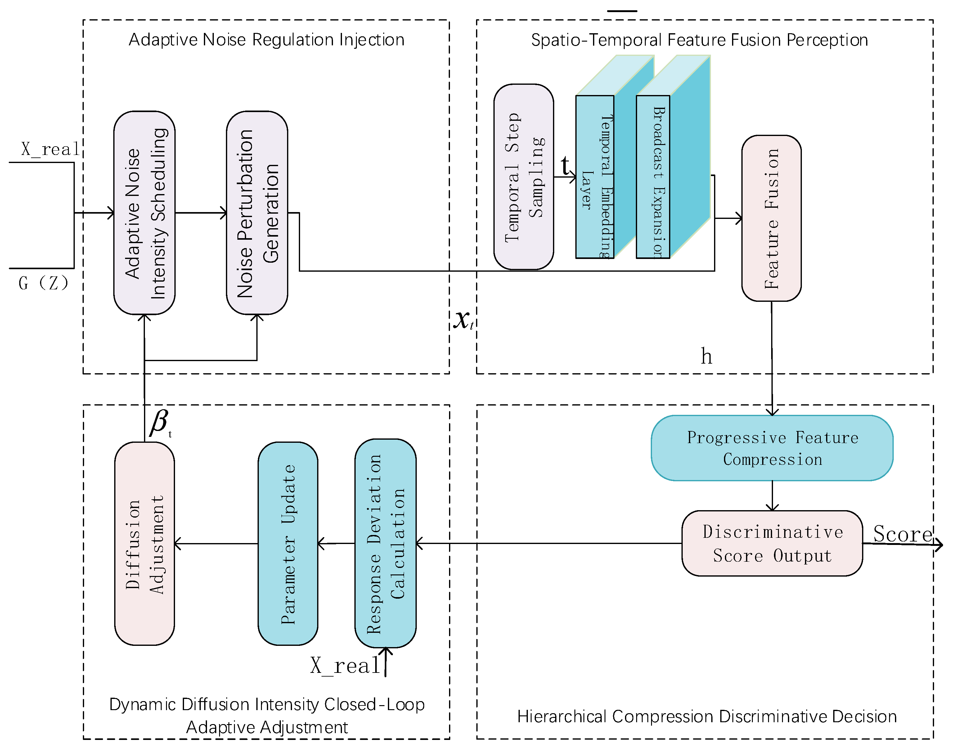
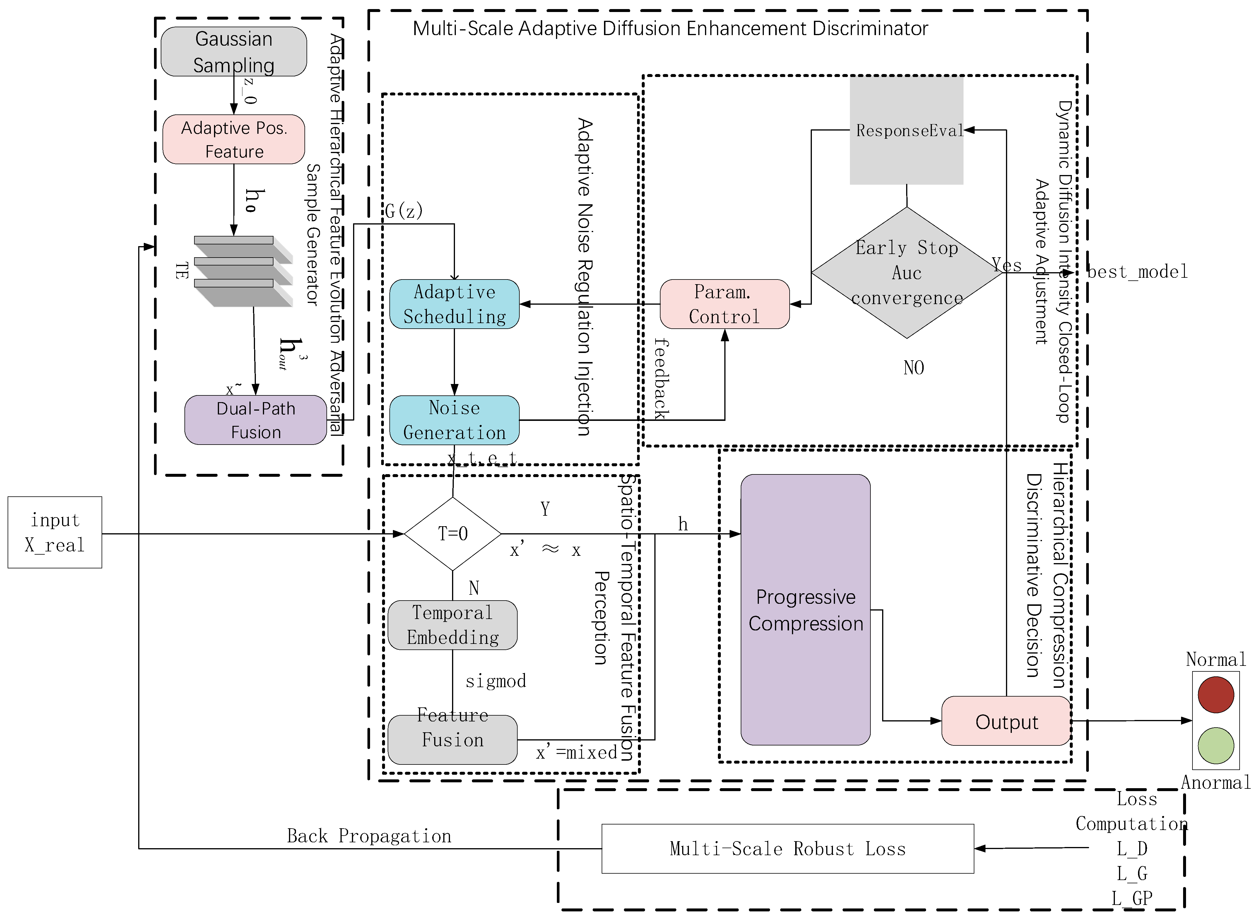
The original tabular data, x, is input into the ADAEN model and processed through three modules: the adaptive hierarchical feature evolution adversarial sample generator (AHFE-Generator), the multi-scale adaptive diffusion enhancement discriminator (MSAD-Discriminator), and the multi-scale robust adversarial gradient loss function (MSAG-Loss), ultimately outputting anomaly detection results, as illustrated in Figure 1. The AHFE generator samples a 128-dimensional latent vector z from a standard Gaussian distribution N(0,I) and generates synthetic samples G(z) with a similar distribution to real data through a hierarchical evolution process involving adaptive attribute-aware high-dimensional feature representation, third-order feature encoding, and dual-path residual fusion feature generation (see Section 2.1). The adaptive noise regulation injection module receives synthetic data, G(z), from the generator and real data, x, applying multi-scale noise perturbations through adaptive noise regulation injection to obtain perturbed data, x_t. Subsequently, this perturbed data, x_t, undergoes deep coupling with diffusion step encoding, e_t, through diffusion-conditional feature fusion perception to yield fused features, h. These fused features, h, are then processed by a hierarchical compression network to output normal or anomalous results. The discriminator’s output serves not only for anomaly identification but also dynamically adjusts the diffusion intensity through a closed-loop feedback mechanism, enabling bidirectional interaction with the generator (detailed in Section 2.2). The MSAG loss function receives discriminative results from the discriminator output and guides high-quality sample generation through Wasserstein adversarial loss, L_D, gradient penalty, L_GP, and generator loss, L_G. Loss signals simultaneously update the generator and discriminator parameters through backpropagation while regulating diffusion intensity to form closed-loop optimization. Early stopping is triggered when AUC shows no improvement for 50 consecutive epochs, outputting the optimal detection model for normal/anomalous classification (see Section 2.3).

2.1. Adaptive Hierarchical Feature Evolution Generator

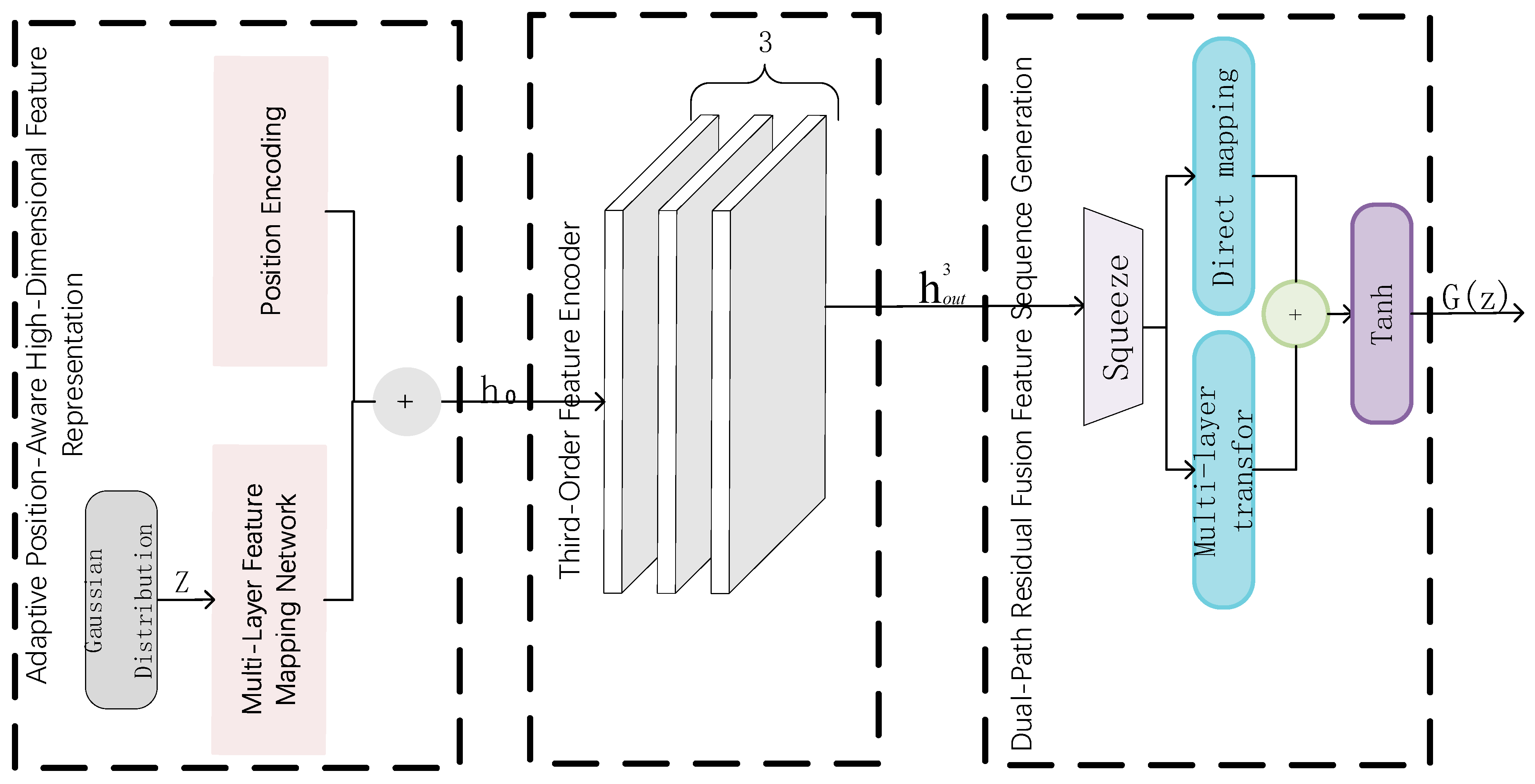
Traditional tabular data generative methods, such as VAEs and standard GANs (e.g., CTGAN), often struggle to capture the complex joint distributions of heterogeneous features. They specifically suffer from mode collapse, training instability, and an inability to model high-order correlations between discrete and continuous attributes. To address these limitations, this paper proposes an adaptive hierarchical feature evolution generator (formerly ‘Evolutionary’). This architecture achieves robust modeling of complex feature dependencies through learnable attribute embeddings (replacing position-aware representation), a third-order feature encoder, and a dual-path residual fusion mechanism, as illustrated in Figure 2.

2.1.1. Adaptive Attribute-Aware High-Dimensional Feature Representation Method

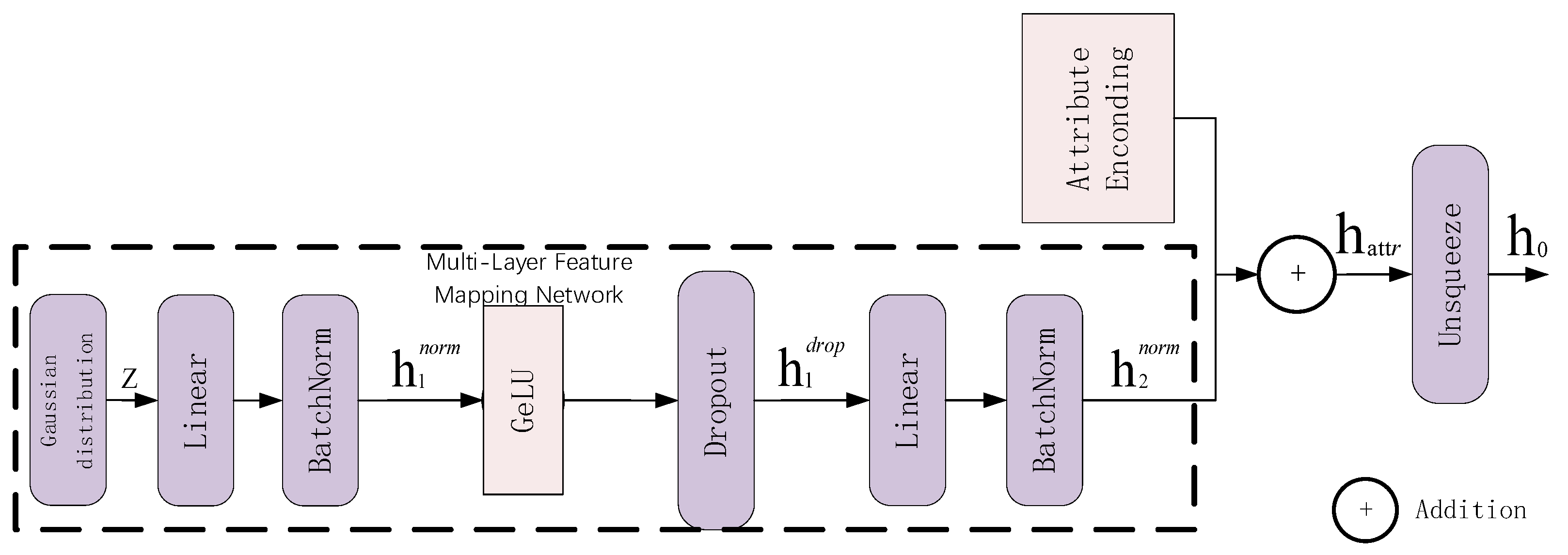
Traditional generation methods adopt fixed encodings and feature transformations, which fail to capture complex inter-feature dependency relationships and suffer from mode collapse issues. Therefore, this paper proposes a learnable attribute-aware high-dimensional feature representation method. This method enables the model to capture and target high-resolution feature representations by adaptively adjusting 128-dimensional normalized vectors through a multi-layer feature distribution network, as illustrated in Figure 3. It outputs standardized intermediate feature vectors, effectively addressing the limitations of fixed encodings in modeling heterogeneous tabular attributes.

(1)

Activation-based high-dimensional feature representation

Mixed activation high-dimensional feature representation is stored in a high-dimensional feature space with fixed activation functions that combine high-dimensional feature spaces. The network learns to adjust this space through multi-layer feature representation learning. After optimization, the obtained standardized intermediate feature, $h^{norm}\in {\mathbb{R}}^{d_5},$ is as shown in Equation (1):

$$h_t^{norm}=\mathrm{BatchNorm}\left(\mathrm{linear}\right(z\left)\right)$$

(1)

The standardized intermediate feature, $h_t^{norm}$, undergoes the Leaky ReLU activation function to introduce the nonlinear transformation capability and applies a Dropout layer for regularization to prevent overfitting and enhance model generalization, as shown in Equation (2):

$$h_t^{drop}=\mathrm{Dropout}(\mathrm{LeakyReLU}(h_t^{norm}))$$

(2)

The feature $h_t^{drop}$ undergoes second-order nonlinear processing and normalization. Through parametric feature mapping and multi-order encoding, the standardized feature dimension $d_{model}=256$ is obtained, yielding a standardized feature, $h_t^{norm}$.

(2)

Adaptive attribute awareness

Unlike traditional Transformers that process ordered token sequences, tabular data consists of heterogeneous attributes (columns) without inherent ordering. To inject structural priors without positional encodings, we introduce learnable attribute embeddings, denoted as P. Instead of using fixed sinusoidal positional encodings, P is initialized as a learnable parameter matrix and optimized jointly with the network to provide a dataset-specific global attribute manifold bias for the tabular feature set. The fusion operation combines the normalized semantic features ${\mathrm{h}}_{norm}$ with P to obtain an attribute-biased representation, ${\mathrm{h}}_{attr}$. This injection of structural information is defined as shown in Equation (3):

$${\mathrm{h}}_{attr}={\mathrm{h}}_{norm}+\mathrm{P}$$

(3)

where P has the same dimensionality as ${\mathrm{h}}_{norm}$. Since the input is a unified latent representation of the entire table row, the learnable attribute embedding P functions as a global manifold bias. P injects a structured inductive bias that helps to align the latent noise vector, z, with the characteristic high-dimensional manifold of the specific tabular dataset, encouraging the generator to satisfy global distributional constraints. Subsequently, $h_{\mathrm{attr}}$ is reshaped for the Transformer block. In our setting, each table row is encoded as a single token ($L=1$, $d_{\mathrm{model}}$). Thus, cross-feature interactions are captured by multi-head projections and FFN/residual evolution, rather than inter-token mixing. The reshaping operation is defined as shown in Equation (4).

$${\mathrm{h}}_0=\mathrm{Unsqueeze}({\mathrm{h}}_{attr},\dim =0)\in {\mathbb{R}}^{1\times d_{model}}$$

(4)

Accordingly, the attention block does not perform inter-token mixing; it acts as a structured multi-subspace projection on a single token.

The proposed learnable attribute-aware representation employs normalization for stable training, enabling precise structural bias injection while maintaining robust feature extraction beyond traditional fixed-encoding methods.

2.1.2. Third-Order Feature Encoder

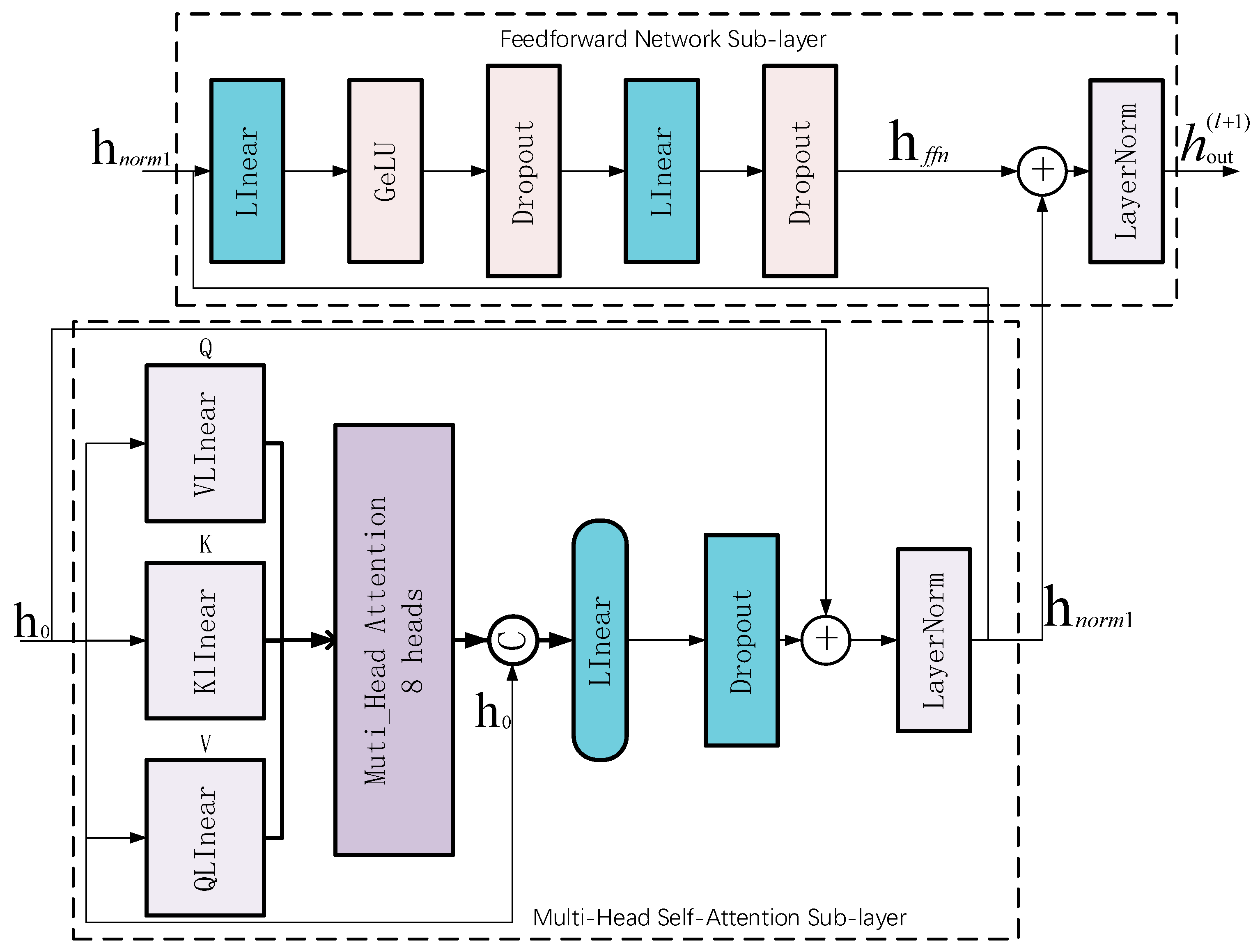
This hierarchical connection originates from the adaptive attribute-aware high-dimensional feature representation $h_0\in {\mathbb{R}}^{1\times d_{model}}$ (where $\mathrm{D}$ is the feature dimension). The three-layer phase-locked structure encoder layers are interconnected, and this layer retrieves high-dimensional feature abstraction at different granularities to yield feature representation, $h_{out}^{\left(3\right)}\in {\mathbb{R}}^{1\times d_{model}}$. Each encoder layer contains multiple self-attention and feedforward network components, as shown in Figure 4.

(1)

Multi-head self-attention layer

The multi-head self-attention layer employs eight attention heads in the standard configuration. However, a critical distinction must be made regarding the operational mechanism of this module in the context of tabular data. ADAEN inputs the feature representation of an entire table row as a unified semantic token ($h_0$), implying a sequence length of $L=1$. Under this condition ($L=1$), the standard scaled dot-product attention mechanism undergoes a functional transformation. The attention weight matrix, typically $\mathrm{softmax}({\displaystyle \frac{Q{K}^T}{\sqrt{d_k}}})$, collapses to a scalar identity, rendering the token-mixing capability redundant. Consequently, the multi-head attention (MHA) module reconfigures from a sequence interaction mechanism into a structured subspace projection ensemble. Mathematically, for the single input vector $z$, the operation of the $i$-th attention head simplifies to a direct linear projection into a specific semantic subspace, as shown in Equation (5):

$${\mathrm{Head}}_i\left(z\right)=z{W}_V^i$$

(5)

where $W_V^i\in {\mathbb{R}}^{d_{model}\times d_{head}}$ represents the learnable projection matrix for the $i$-th head. The architecture relies on the parallelization of these heads to capture diverse feature representations. The outputs are concatenated and fused via a linear transformation, $W_O$, as defined in Equation (6):

$$\mathrm{MHA}\left(z\right)=\mathrm{Concat}\left({\mathrm{Head}}_1\right(z),\dots ,{\mathrm{Head}}_h(z\left)\right)W_O$$

(6)

This structure serves a crucial role that is distinct from simple dense layers: it acts as a low-rank constraint regularizer. By forcing the generator to decompose the high-dimensional latent information into $h$ independent subspaces (8 heads in our configuration) before fusion, the model is compelled to learn a mixture of distinct viewpoints of the data manifold. This effectively mitigates the mode collapse that is often observed in wide, unstructured, fully connected networks when generating heterogeneous tabular data. Furthermore, the non-linearity required for complex manifold modeling is preserved and enhanced by the subsequent position-wise feed-forward network (FFN) and residual connections. The complete evolution of the feature vector $z$ through one encoder layer is defined in Equations (7) and (8):

$$z^{\prime }=\mathrm{LayerNorm}(z+\mathrm{MHA}(z\left)\right)$$

(7)

$$z_{out}=\mathrm{LayerNorm}(z^{\prime }+\mathrm{FFN}(z^{\prime }\left)\right)$$

(8)

Through this deep residual feature evolution process, the generator progressively refines the latent noise into high-fidelity tabular samples, leveraging the structured projection ensemble to maintain feature diversity.

(2)

Feedforward network layer

The feedforward network layer performs a nonlinear transformation on the features, $h_{norm1}$, after first-order processing. $h_{norm1}$ undergoes a nonlinear transformation through successive linear layers, GELU activation, Dropout regularization, secondary nonlinear transformation, and Dropout processing to yield $h_{ffn}$, as shown in Equation (9):

$$h_{ffn}=\mathrm{Dropout}\left(\mathrm{linear}\right(\mathrm{Dropout}\left(\mathrm{GELU}\right(\mathrm{linear}\left(h_{norm1}\right)\left)\right)\left)\right)$$

(9)

$h_{ffn}$ and $h_{norm1}$ undergo residual connection and layer normalization to obtain the encoder layer output $h_{out}$, as shown in Equation (10):

$$h_{out}=\mathrm{LayerNorm}(h_{norm1}+h_{ffn})$$

(10)

(3)

Third-order framework structure

Three phase-locked encoder layers perform hierarchical feature extraction and dimensionality compression, as shown in Equation (11):

$$h_{out}^{(l+1)}=\mathrm{EncoderLayer}(h_{out}^{\left(l\right)}), l=\mathrm{0,1},2$$

(11)

where $h_{out}^1=h_0$ serves as the initial input and $h_{out}^3$ represents the output of the third-order encoding layer. The encoder’s first layer focuses on different granularities of feature patterns, the encoder’s second layer focuses on semantic attention feature interactions and dimensional suppression layer patterns, and the encoder’s third layer can extract global semantic information and high-resolution feature representation.

2.2. Multi-Scale Adaptive Diffusion Enhancement Discriminator Architecture

The existing anomaly detection methods adopt fixed noise strategies and lack diffusion–discrimination collaborative mechanisms, resulting in the models’ inability to dynamically adjust noise levels based on discriminator feedback. This limitation restricts the multi-scale feature learning capability and detection accuracy. Therefore, a multi-scale adaptive diffusion enhancement discriminator is proposed, primarily consisting of four components: adaptive noise regulation injection, diffusion-conditional feature fusion perception, hierarchical compression discriminative decision-making, and dynamic diffusion intensity closed-loop adaptive adjustment, as shown in Figure 5. The adaptive noise regulation injection receives original data (Xreal) and generated data (G(z)), generating samples with different perturbation levels through noise intensity control (detailed in Section 2.2.1). These perturbed samples, together with the corresponding diffusion step encoding (t), are input into the diffusion-conditional feature fusion perception module to produce fused features (h), enabling the model to acquire a noise-level-aware discrimination capability (detailed in Section 2.2.2). The fused features (h) are sent to the hierarchical compression discriminative decision module, which outputs anomaly scores (D(x,t)) after layer-by-layer processing (detailed in Section 2.2.3). The anomaly scores are fed back to the dynamic diffusion intensity closed-loop adaptive module, which adjusts noise parameters ${\beta }_t$ accordingly and returns them to the adaptive noise injection module, thereby forming a closed-loop optimization mechanism (detailed in Section 2.2.4).

2.2.1. Adaptive Noise Regulation Injection Mechanism

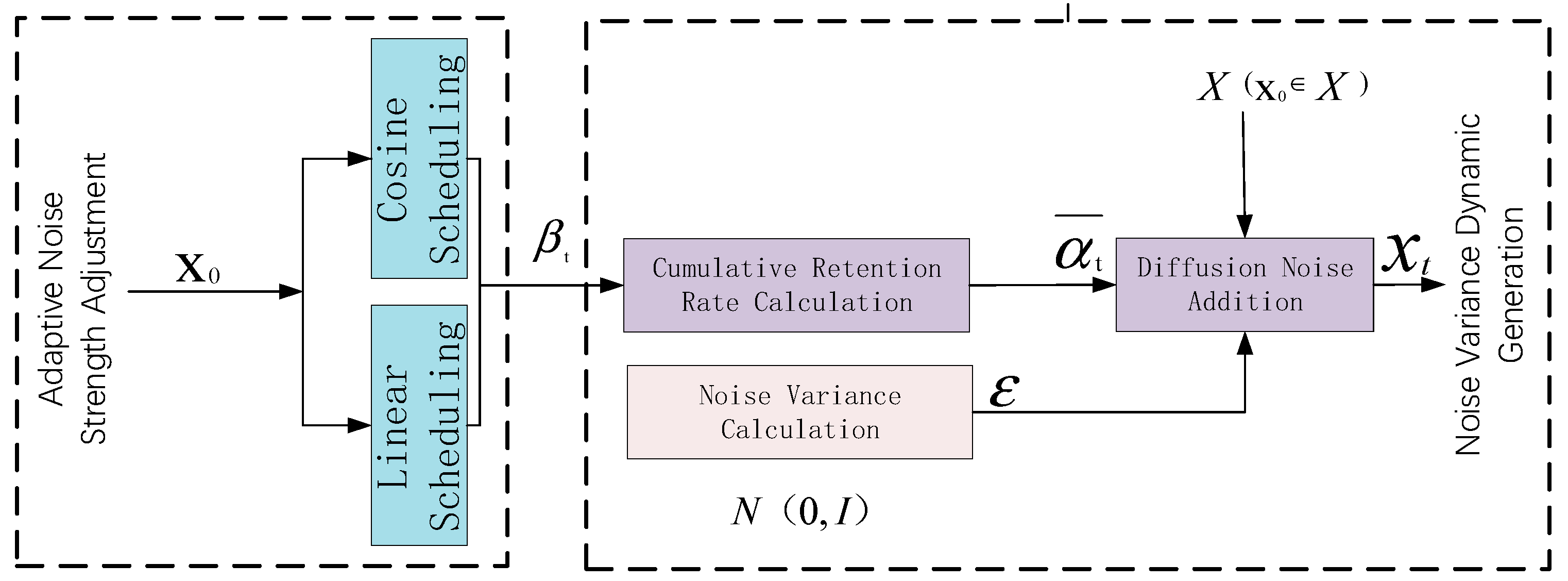
Traditional anomaly detection methods adopt fixed noise variance strategies, which cannot adjust according to data characteristics and training dynamic states to achieve appropriate granularity, thereby limiting the models’ adaptive ability. Therefore, this paper proposes an adaptive noise regulation injection mechanism that achieves different gradient capability reflections through controllable noise dynamic adjustment and variance dynamic adjustment. This mechanism dynamically maintains optimal granularity while preserving high-dimensional semantic features during processing for effective noise timing disclosure. By optimizing score-controllable diffusion response strength within the adaptive framework, it enhances the target model’s discriminative ability to prevent insufficient noise information. The design enables two requirements: adaptive response strength adjustment and bidirectional optimization of the noise strength dynamic response, as shown in Figure 6.

(1)

Adaptive noise strength adjustment

This section implements a dual-mode adaptive noise adjustment mechanism that enables dynamic switching based on data distribution characteristics for online and conditional adjustment. When the data distribution employs the mean conditional adjustment for variance-based adaptive adjustment to achieve gradient-based noise selection, specific regulation is defined as shown in Equation (12). The base schedule shape is defined here to distinguish between linear and non-uniform distributions, as shown in Equation (13):

$${\beta }_t={\beta }_{start}+\mathcal{S}\left(t\right)·({\beta }_{end}-{\beta }_{start})$$

(12)

where $\mathcal{S}\left(t\right)$ is determined by the following data distribution:

$$\mathcal{S}(t)=\left\{\begin{array}{cc}{\displaystyle \frac{t}{T_{max}}}& \mathrm{if} x_0\mathrm{is} \mathrm{uniform} \left(\mathrm{Linear}\right)\\ 1-\mathrm{c}\mathrm{o}\mathrm{s}\left({\displaystyle \frac{\pi t}{2T_{max}}}\right)& \mathrm{if} x_0 \mathrm{is} \mathrm{non-uniform} \left(\mathrm{Cosine}\right)\end{array}\right.$$

(13)

where ${\beta }_{start}=0.0001$, ${\beta }_{end}=0.02$, and $T_{max}$ represents the maximum diffusion step count (set to 100).

(2)

Noise variance dynamic generation

Noise adjustment enables the expression of dynamic noise strength for multi-dimensional representation at different noise strength diffusion stage distributions. ${\alpha }_t=1-{\beta }_t$ small noise strength maintains local partial details, while a large noise strength extracts global distributional characteristics. Based on the noise variance coefficient, the single-step retention rate is maintained. The cumulative retention rate at diffusion step $t$ follows a uniform distribution $U(1,T_{max})$, where $T_{max}$ is the maximum diffusion step count.

Subsequently, the cumulative retention rate, ${\overline{\alpha }}_t=\prod _{i=1}^t{\alpha }_i$, is calculated, where ${\alpha }_i$ represents the retention rate at the $i$-th step, $({\alpha }_i=1-{\beta }_i)$. ${\beta }_i$ represents the noise variance at the $i$-th step. The sampled noise, $ϵ$, follows a standard high-variance Gaussian distribution $N(0,I)$, enabling parameterized quantification to achieve high-quality sampling and normalization implementation, as shown in Equation (14):

$$x_t=\sqrt{{\overline{\alpha }}_t}·x_0+\sqrt{1-{\overline{\alpha }}_t}·ϵ$$

(14)

where $ϵ\sim N(0,I)$ represents standard high-variance noise and $x_0$ represents the input data for diffusion processing initialization. In actual training, x₀ represents the input data for diffusion processing, which can be either real data, X_real, or generated data, G(z), from the generator, enabling the diffusion process to be equally applicable to both data types and providing the discriminator with diversified training samples. This unified representation enables diffusion processing to be equally applicable to both real and generated samples, providing the discriminator with diversified training data.

2.2.2. Diffusion-Conditional Feature Fusion Perception Module

Current discriminators lack effective integration of feature characteristics and diffusion step information, which limits their perceptual ability under varying noise levels and restricts the accuracy of multi-dimensional anomaly detection. Therefore, a diffusion-conditional feature fusion perception method is proposed. This method achieves deep coupling of diffusion step information and data features through learnable diffusion step embedding and feature-wise conditional operations to facilitate the deep integration of diffusion step information and data features. This design not only preserves the original distributional characteristics of the data but also enables the discriminator to acquire a noise-level-aware perceptual ability, thereby enhancing anomaly detection accuracy across different diffusion stages, as shown in Figure 7.

(1)

Diffusion step embedding integration

Diffusion step embedding obtains learnable embeddings through learnable embedding matrices (these matrices are initialized using a random Gaussian distribution and optimized through training dynamics to capture diffusion stage information). The specific mapping from diffusion step $t$ to D-dimensional continuous vector representation $e_t\in {\mathbb{R}}^D$ is shown in Equation (15), where D denotes the embedding dimension. This operation achieves diffusion-stage-aware encoding.

$$e_t=\mathrm{Embedding}\times t$$

(15)

The diffusion step $x_t\in {\mathbb{R}}^{B\times D}$ undergoes a sinusoidal calculation to represent the standardized tensor format. Diffusion step embedding $X_e\in {\mathbb{R}}^D$ undergoes dimension matching with diffusion feature tensors, $x_t$, for feature dimension determination processing, ensuring $\dim \left(x_t\right)=\dim \left(e_t\right)=D$. For gradient calculation and handling batch-wise Diffusion step embedding and expansion feature correlation, $X_t$, see Equation (16):

$$E_t=e_t\otimes 1_{B\times 1}$$

(16)

This broadcast operation achieves and replicates the diffusion step embedding, $e_t$, through batch dimension construction, resulting in tensor form $B\times D$ embedding matrices. The batch dimension tensor processing system is denoted as $E_t[i,:]=e_t,i\in \{1:B\}$.

(2)

Diffusion-conditional feature integration

$E_t$ (encoding diffusion stage information matrices) and diffusion data features $x_t$ (data representation after noise injection at diffusion step t) undergo concatenation to form diffusion-conditioned features, $h$, as shown in Equation (17):

$$h=x_t+E_t$$

(17)

2.2.3. Hierarchical Compression Discriminative Decision

Traditional discriminators adopt complex deep network structures with excessive parameters and computational overhead during anomaly detection tasks, which directly leads to high-dimensional mapping and a loss of associated feature information, thereby affecting anomaly detection accuracy. Therefore, a hierarchical compression discriminative decision strategy is proposed to achieve high-efficiency anomaly evaluation through the discriminative strategy decision processing from two key hierarchical organizations, as shown in Figure 8.

(1)

Gradient-style feature compression

Gradient-style feature compression achieves full-connection layer mapping processing through learned high-dimensional encoding. This processing extracts discriminative features from the high-dimensional encoding, as shown in Equation (18):

$$z_1=\mathrm{FC}\left(h\right)$$

(18)

$z_1$ undergoes the LeakyReLU activation function to introduce nonlinearity and passes through a Dropout layer for random inactivation to obtain regularized features, $a_1$, as shown in Equation (19):

$$a_1=\mathrm{Dropout}\left(\mathrm{LeakyReLU}\right(z_1\left)\right)$$

(19)

After regularization, $a_1$ is again input to the fully connected (FC) layer, undergoing nonlinear transformation, LeakyReLU activation, Dropout regularization, and an identical processing flow to obtain $a_2$. This hierarchical compression processing ensures feature extraction while preventing gradient explosion and overfitting.

(2)

Discriminative evaluation output

The discriminative evaluation output achieves compression from $a_2$ to feature mapping for anomaly evaluation. Features, $a_2$, undergo FC layer mapping processing to obtain the dimension, $z_2$, as shown in Equation (20):

$$z_2=\mathrm{FC}\left(a_2\right)$$

(20)

$z_2$ undergoes sigmoid function normalization to output an anomaly probability score, as shown in Equation (21):

$$\mathrm{score}=\mathrm{Sigmoid}\left(z_2\right)$$

(21)

This score value falls within the [0, 1] interval, directly representing the samples’ anomaly probability.

2.2.4. Dynamic Diffusion Intensity Closed-Loop Adaptive Adjustment

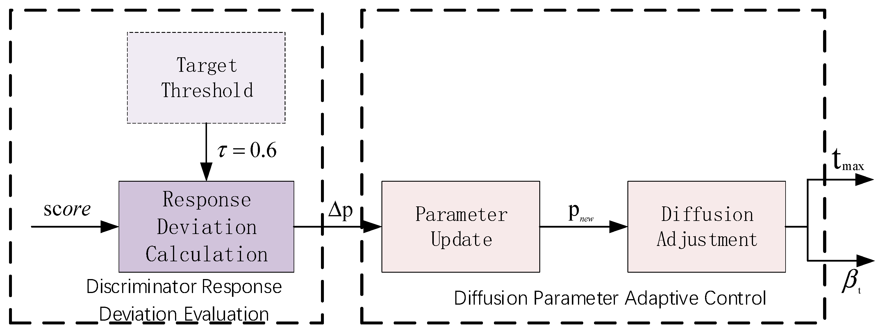
The current diffusion models adopt fixed noise variance parameters and lack discriminator feedback mechanisms, resulting in fixed noise schedules that cannot dynamically adjust noise levels based on model performance and training status across different training stages and datasets, thus limiting self-adaptive capability. Therefore, a closed-loop adjustment self-adaptive control method is proposed that enables the dynamic adjustment of diffusion parameters through dynamic training feedback of discriminator performance. Dynamic diffusion intensity self-adaptive adjustment consists of four key hierarchical components, as shown in Figure 9: discriminator response evaluation, preset target response adaptive threshold calculation, diffusion parameter self-adaptive adjustment, and closed-loop feedback control.

(1)

Discriminator response evaluation

The discriminator response evaluation estimates the discriminator’s response confidence to real data. The discriminator obtains the output value, $D\left(x\right)$, from real data, $X_{real}$, to estimate $R_{real}$, which evaluates its discriminative capability. This process provides discriminative confidence and can adjust its strategy to offer foundational information. The discriminator response evaluation process is defined as shown in Equation (22):

$$R_{real}={\mathbb{E}}_{x\sim p_{data}}\left[D\left(x,t_0\right)\right]$$

(22)

This variable reflects the average response value of the discriminator to real data, serving as a fundamental reference for subsequent adjustments. Higher $R_{real}$ values indicate that the discriminator has a stronger capability to recognize real data.

The present target response value calculation bias, $\Delta p$, is shown in Equation (23):

$$\Delta p=\mathrm{sign}(R_{real}-\tau )·C$$

(23)

where $C$ is the length factor for controlling adjustment amplitude. This calculation of $\Delta p$ determines the adjustment direction and magnitude for diffusion strength. When $R_{real}$ is higher than the target response threshold value $\tau$, the system will increase diffusion strength; when $R_{real}$ is lower than the $\tau$, the system will reduce the diffusion strength. It is generally set to 0.6.

(2)

Diffusion parameter self-adaptive adjustment

Diffusion parameter self-adaptive adjustment performs adaptive parameter updates for enhanced style feature updating. In the specific implementation, this method adjusts the previous step’s noise adjustment degree, $p_{old}$, and the current calculated estimated noise processing parameter, $p_{new}$. While maintaining performance within the effective range [0, 1], this interval prevents excessive diffusion and maintains the maximum diffusion strength to achieve parameter balance and optimization. Parameter updates are implemented as shown in Equation (24):

$$p_{new}=\mathrm{clip}(p_{old}+\Delta p,\mathrm{0,1})$$

(24)

Adaptive parameter dynamic adjustment maintains parameter $p_{new}$ for transmission to diffusion adjustment and completes the feedback-controlled system process, as shown in Equation (25):

$$t_{max}=p_{new}·T_{max}$$

(25)

where $T_{max}$ is the preset maximum diffusion step count, diffusion processing will adopt diffusion steps within the range during diffusion step selection, thereby achieving controlled diffusion parameter adjustment.

This design preserves the adjustment of the noise strength control parameter by scaling the base schedule, $\mathcal{S}\left(t\right)$, as shown in Equation (26). The controllable parameter, $p_{new}$, serves as the diffusion intensity scaling factor, enabling more refined control:

$${\beta }_t=p_{new}·{\beta }_{start}+\mathcal{S}\left(t\right)·({\beta }_{end}-{\beta }_{start})$$

(26)

For the default configuration using the cosine schedule, this expands to Equation (27):

$${\beta }_t=p_{new}·{\beta }_{start}+\left(1-\cos \left({\displaystyle \frac{\pi t}{2T_{\max }}}\right)\right)·({\beta }_{end}-{\beta }_{start})$$

(27)

This adaptive adjustment mechanism, as defined in Equations (26) and (27), enables the diffusion process to dynamically control the noise strength, ${\beta }_t$, based on training feedback, facilitating optimal balance between model performance and data representation capability.

2.3. Multi-Scale Robust Adversarial Gradient Loss Function

Existing anomaly detection loss functions lack multi-scale adaptability and exhibit gradient instability during adversarial training, preventing models from maintaining robust detection performance across varying noise levels. To address this issue, a multi-scale robust adversarial gradient loss function is proposed. This loss function optimizes the algorithm through alternating training between the discriminator and generator. The loss function comprises the Wasserstein adversarial loss, ${\mathcal{L}}_D$, gradient penalty loss, ${\mathcal{L}}_{GP}$, and generator optimization loss, ${\mathcal{L}}_G$, as shown in Equation (28).

$$\begin{array}{c}{\mathcal{L}}_{total}=\left\{\begin{array}{c}{\mathcal{L}}_D+{\lambda }_{GP}{\mathcal{L}}_{GP} \mathit{discriminator\_phase}\\ {\mathcal{L}}_G \mathit{generator\_phase}\end{array}\right.\end{array}$$

(28)

where ${\lambda }_{GP}$ represents the weight parameter.

Wasserstein adversarial loss: This adversarial loss constructs multi-scale discriminative objectives through diffusion-step-conditioning. The loss function maximizes the discriminator’s response to real data while minimizing its response to generated data across different diffusion stages, enabling the discriminator to learn the distributional differences between real and generated data at multiple noise levels, thereby effectively enhancing the model’s capability to discriminate anomaly patterns at different scales. The loss L_D is defined in Equation (29).

$$\begin{array}{c}{\mathcal{L}}_D=-{\mathbb{E}}_{\mathbf{x}\sim p_{data}}\left[D\left(\mathbf{x},t_0\right)\right]+{\mathbb{E}}_{\mathbf{z}\sim p_z,t\sim P\left(t\right)}\left[D\left(\mathrm{Diffusion}\left(G\left(\mathbf{z}\right),t\right),t\right)\right]\end{array}$$

(29)

where $t_0=0$ represents the diffusion step of the original data, and $\mathrm{Diffusion}\left(G\left(\mathbf{z}\right),t\right)$ denotes the generated data after t steps of diffusion. Here, ${\mathbb{E}}_{\mathbf{x}\sim p_{data}}$ denotes the mathematical expectation over samples $p_{data}$ sampled from the real data distribution, $\mathbf{x}$, and ${\mathbb{E}}_{\mathbf{z}\sim p_z,t\sim P\left(t\right)}$ denotes the joint expectation over latent vectors, $\mathbf{z}$, sampled from the standard Gaussian distribution $P\left(t\right)=\mathrm{Uniform}(1,T_{max})$ and diffusion steps, $t$, sampled from the uniform distribution, U(0,T).

Gradient penalty loss: The gradient penalty loss enforces soft constraints on the discriminator to satisfy the Lipschitz continuity condition, which constrains the L2 norm of the discriminator’s gradient to be close to 1, thereby ensuring that the gradient remains bounded at any point in the sample space. This effectively prevents the gradient explosion or vanishing problem during adversarial training. The loss, ${\mathcal{L}}_{GP}$, is defined in Equation (30).

$${\mathcal{L}}_{GP}={\mathbb{E}}_{\widehat{\mathbf{x}}\sim P_{\widehat{\mathbf{x}}}}[{\left(\parallel {\nabla }_{\widehat{\mathbf{x}}}D\left(\widehat{\mathbf{x}},\widehat{t}\right){\parallel }_2-1\right)}^2]$$

(30)

where ${\nabla }_{\widehat{\mathbf{x}}}D\left(\widehat{\mathbf{x}},\widehat{t}\right)$ represents the gradient of the discriminator at the interpolated point, as shown in Equation (31). It reflects the rate of change in the discriminator’s output with respect to the input.

$${\nabla }_{\widehat{\mathbf{x}}}D\left(\widehat{\mathbf{x}},\widehat{t}\right)={\displaystyle \frac{𝜕D\left(\widehat{\mathbf{x}},\widehat{t}\right)}{𝜕\widehat{\mathbf{x}}}}$$

(31)

where $\widehat{\mathbf{x}}$ represents the interpolated data point constructed between real data, X_real, and generated data, G(z), obtained through linear combination, as shown in Equation (32).

$$\widehat{\mathbf{x}}=\alpha \mathrm{X\_real}+(1-\alpha )\mathrm{G}\left(\mathrm{z}\right)$$

(32)

where in Equation (32), $\alpha \sim \mathrm{Uniform}\left(\mathrm{0,1}\right)$ is a random coefficient sampled from a uniform distribution. This random interpolation strategy ensures that the gradient penalty is uniformly distributed across the entire data manifold.

Equation (33) indicates that the interpolated diffusion step, $\widehat{t}$, is constructed between the real data diffusion step, t_real, and the generated data diffusion step, t_fake. This diffusion step is obtained through linear combination and is used in conjunction with the downsampling operation to ensure numerical stability, as shown in Equation (33).

$$\widehat{t}=\lfloor \alpha t_{real}+(1-\alpha )t_{fake}\rfloor$$

(33)

Additionally, Equation (34) ensures that ${\nabla }_{\widehat{\mathbf{x}}}D\left(\widehat{\mathbf{x}},\widehat{t}\right)$ satisfies the Lipschitz constraint, as shown in Equation (34).

$$\parallel {\nabla }_{\mathbf{x}}D\left(\mathbf{x},t\right){\parallel }_2\le 1,\forall \mathbf{x},t$$

(34)

This soft constraint is more robust compared to hard constraints. While ensuring training stability, it allows for a certain degree of gradient variation, effectively enforcing the Lipschitz continuity of the discriminator.

Generator loss: High-dimensional features present challenges for adversarial training, which often fails to provide stable gradient signals. To address this, the Wasserstein distance is introduced to optimize the generation process, as the generated data distribution has real properties. L_G can be expressed as Equation (35).

$$\begin{array}{c}{\mathcal{L}}_G=-{\mathbb{E}}_{\mathbf{z}\sim p_z,t\sim P\left(t\right)}\left[D\left(\mathrm{Diffusion}\left(G\left(\mathbf{z}\right),t\right),t\right)\right]\end{array}$$

(35)

where G(z) represents the generator’s output. This loss encourages the generator to produce high-quality data that can effectively deceive the discriminator.

Threshold determination strategy: To ensure a rigorous comparison that is consistent with the established benchmarks [39], we employ the best F1-Score (F1-Max) strategy. This protocol selects the optimal threshold ${\tau }^{\mathrm{*}}$ that maximizes the F1-Score on the test set, thereby evaluating the models’ intrinsic discriminative capability, independent of specific thresholding heuristics. The optimal threshold is defined as Equation (36):

$${\tau }^{\mathrm{*}}=\underset{\tau }{argmax}F1(\tau )=\underset{\tau }{argmax}\left(2·{\displaystyle \frac{P\left(\tau \right)·R\left(\tau \right)}{P\left(\tau \right)+R\left(\tau \right)}}\right)$$

(36)

where $P\left(\tau \right)$ and $R\left(\tau \right)$ denote the precision and recall at threshold $\tau$.

2.4. Theoretical Advantages over State-of-the-Art Baselines

ADAEN is explicitly designed to overcome the inductive bias limitations of the existing frameworks (summarized in

Table 1. Theoretical comparison of ADAEN with competitive frameworks.

Model	Core Mechanism	Primary Inductive Bias	Critical Limitation on Tabular Data	Computational/Modeling Characteristic
LOF	Density-based k-NN	Local density continuity	Curse of dimensionality: Distance metrics fail in high-dim space.	Pairwise distance computation; scalability degrades rapidly with feature dimensionality
Deep SVDD	One-class Neural Network	Unimodal Hypersphere	Hypersphere collapse: Struggles with multi-modal/multi-cluster data.	Single-stage deep representation learning; moderate training cost, efficient inference
MO-GAAL	Multi-Generator GAN	Minimax Game	Training instability: Prone to mode collapse and gradient vanishing.	Multi-generator adversarial training; high training overhead and sensitivity to hyperparameters
DiffusionAD	DDPM/Denoising	Fixed Noise Schedule	Rigidity: Fixed noise corrupts heterogeneous features (discrete/continuous).	Iterative denoising inference; high inference latency proportional to diffusion steps
Mamba-AD	State Space Model (SSM)	Sequential Scan	Sequence bias: Imposes false order on permutation-invariant columns.	Linear-complexity state-space scanning; highly efficient but order-sensitive
ADAEN (Ours)	Diffusion Adversarial Network with Attention	Global feature interaction modeling	Increased cost for high-dimensional feature interactions.	Attention-based feature modeling with quadratic interaction cost; single-pass inference after training

). Unlike LOF [40], which suffers from the “curse of dimensionality” and distance concentration in raw feature spaces, ADAEN detects anomalies within a learned lower-dimensional latent manifold via the AHFE generator. In contrast to Deep SVDDs [41] unimodal hypersphere assumption, which risks mode collapse on multi-modal tabular distributions, ADAEN’s adversarial framework naturally captures complex, non-convex data topologies. Furthermore, ADAEN ensures training stability that is superior to MO-GAAL [42] via the MSAG loss (Wasserstein distance with gradient penalty) and addresses the feature heterogeneity that is often mishandled by DiffusionADs [43] fixed noise schedules through the MSAD discriminators closed-loop feedback regulator. Finally, while Mamba-AD [44] offers linear computational complexity (O(L)), it imposes incorrect sequential biases on permutation-invariant tabular data. ADAEN utilizes attention mechanisms to model global feature correlations without positional constraints, achieving superior detection accuracy (average 8.3% AUC improvement) at the expense of moderately higher computational cost due to quadratic feature-interaction modeling, compared to Mamba-AD’s linear state-space scanning.

Table 1 summarizes the key differences between ADAEN and the aforementioned benchmark methods in terms of core mechanisms, manifold assumptions, and high-dimensional data-handling capabilities.

3. Experimental Results and Analysis

3.1. Datasets

The proposed anomaly detection method in tabular data is trained and validated on datasets containing both normal and abnormal samples. This paper employs 14 widely used static anomaly detection benchmark datasets for experimental validation, sourced from the UCI machine learning database.

The experimental datasets are Pima, Shuttle, Stamps, PageBlocks, PenDigits, Annthyroid, Waveform, WDBC, Ionosphere, SpamBase, APS, Arrhythmia, HAR, and p53Mutant. These 14 datasets cover diverse application domains, including medical diagnosis, image recognition, text classification, and network security. The feature dimensions range from 8 to 5408, with sample sizes varying from 150 to 20,000. These samples are treated as independent and identically distributed observations without temporal dependencies.

This paper categorizes the 14 datasets by dimensions into three groups for comparative performance evaluation. Low-dimensional datasets (dimension < 20) include Pima (eight dimensions), Shuttle (nine dimensions), and Stamps (nine dimensions). Medium-dimensional datasets (dimension 20–100) include Waveform (21 dimensions), WDBC (30 dimensions), Ionosphere (32 dimensions), and SpamBase (57 dimensions). High-dimensional datasets (dimension > 100) include APS (170 dimensions), Arrhythmia (279 dimensions), HAR (561 dimensions), and p53Mutant (5408 dimensions).

3.2. Experimental Implementation

Experimental Environment: The experimental hardware environment employs NVIDIA GeForce RTX 4060 Laptop GPU graphics card (NVIDIA, Santa Clara, CA, USA) with 8 GB storage space. The CPU model is an Intel(R) Core(TM) i5-10300H processor (Intel, Santa Clara, CA, USA) with main frequency 2.50 GHz. The system memory is 16 GB. The operating system adopts Windows 10 and Python (version 3.5). The deep learning framework uses PyTorch(version 2.0.0) and employs CUDA and GPU optimization acceleration.

Training parameter configuration: This paper conducts comparative experiments on 14 widely used anomaly detection benchmark datasets, using the proposed Transformer-based anomaly detection model for training. Models are dynamically adjusted according to the dataset scales, with the batch size set to 32 or 64. Training adopts the Adam gradient descent learning rate strategy. The initial learning rates for the generator and discriminator are set to 0.0001. Model training lasts 300–500 epochs, followed by feature dependency discriminator anomaly detection evaluation. The diffusion model adopts a fixed scheduling strategy with values linearly increasing from 0.0001 to 0.02. Diffusion step ranges from 10 to 100. The Transformer generator’s attention head count is set to eight, the encoder layer count is three, and the feedforward network dimension is 512 for effective extraction of feature representations. All models employ the Adam optimizer with parameter settings (\beta_1 = 0.5), (\beta_2 = 0.999). Training processes adopt network regularization strategies with a cutoff threshold set to 1.0. Discriminator dropout rates are set to 0.3 to avoid overfitting. Models employ early stopping: when AUC metrics show no improvement for 50 consecutive epochs exceeding 0.001, training automatically terminates.

Noise schedule configuration:

Table 2. Noise schedule and hyperparameter configuration across experiments. Note: The minus sign (−) indicates not applicable.

Experiment Group	Datasets	Base Schedule Shape S(t) (Equation (13))	Adaptive Feedback (pnew)	Hyperparameters (βstart, βend, τ)
Main Performance	Pima, Shuttle, Stamps (<20 dims)	Linear	Enabled (Dynamic)	10−4, 0.02, 0.6
	Waveform, WDBC, SpamBase (20–100 dims)	Cosine	Enabled (Dynamic)	10−4, 0.02, 0.6
	Arrhythmia, p53Mutant, HAR (>100 dims)	Cosine	Enabled (Dynamic)	10−4, 0.02, 0.6
Ablation Study 1	PenDigits (Strategy Comparison)	5 variants tested: None (baseline)/Linear/Quadratic/Sigmoid/Cosine	Disabled (Fixed p = 1.0 for diffusion variants; N/A for baseline)	10−4, 0.02, −
Ablation Study 2	Arrhythmia (Intensity Analysis)	Cosine (fixed)	4 variants tested: None/Fixed p = 1.0/Fixed p = 0.5/Adaptive	10−4, 0.02, 0.6

details the specific noise strategies for each experiment. We employ the linear schedule (Equation (13)) for low-dimensional uniform datasets and the cosine schedule for complex medium-to-high dimensional data to preserve semantic features. Adaptive feedback (Equations (23)–(26)) is enabled for all main comparisons (Table 2) to dynamically optimize the global intensity scalar, $p_{new}$. Table 2 is the configuration of noise schedules and adaptive feedback for experiments.

3.3. Metrics

Evaluation metrics: For anomaly detection tasks, the ROC curve area (AUC, area under the ROC curve), accuracy, precision, recall, and F1-Score are quantitatively employed to evaluate the proposed method’s performance.

AUC calculates the true positive rate, $TPR$, and the false positive rate, $FPR$, at different threshold values, as shown in Equation (37). This metric is insensitive to class imbalance and is particularly suitable for anomaly detection tasks:

$$AUC={\int }_0^{1}TPR(FP{R}^{-1}(x))dx$$

(37)

AUC metric values range from [0, 1], with higher values indicating better model performance.

Accuracy calculates the proportion of correct predictions made by the model, computing the ratio of correctly predicted anomalous samples, $TP$, and normal samples, $TN$, to total samples, as shown in Equation (38):

$$Accuracy={\displaystyle \frac{TP+TN}{TP+TN+FP+FN}}$$

(38)

where $FP$ represents false positive samples, i.e., incorrectly identified anomalous normal samples. $FN$ represents false negative samples, i.e., incorrectly identified normal anomalous samples.

Precision calculates the proportion of true anomalous samples among samples predicted as being anomalous by the model, primarily reflecting the model’s accuracy capability, as shown in Equation (39):

$$Precision={\displaystyle \frac{TP}{TP+FP}}$$

(39)

Recall calculates the proportion of correctly identified $TP$ among all anomalous samples, $TP+FN$, as shown in Equation (40). This metric reflects the model’s completeness capability:

$$Recall={\displaystyle \frac{TP}{TP+FN}}$$

(40)

The F1-Score represents the harmonic mean of the precision and recall, as shown in Equation (41). This metric comprehensively considers both model accuracy and completeness. When both precision and recall are high, the F1-Score will be high:

$$F1\_Score=2\times {\displaystyle \frac{Precision\times Recall}{Precision+Recall}}$$

(41)

3.4. Performance Comparison and Analysis

3.4.1. Decision Boundary Visualization Analysis

In anomaly detection tasks, the decision boundary is the boundary surface that distinguishes between normal and abnormal samples. It defines which regions in the feature space belong to normal patterns and which regions should be identified as anomalous. Unlike traditional classification tasks, anomaly detection primarily challenges learning an accurate decision boundary based on normal samples alone. When normal data distribution encompasses both rising and surrounding unknown regions, the proposed ADAEN method learns the complex distribution patterns of normal samples through adaptive hierarchical feature evolution and utilizes discriminator–diffusion cooperative models to optimize decision boundaries at multiple scales, achieving stability and robustness through adaptive response loss function boundary optimization. This enables accurate detection of various anomaly patterns. The effectiveness of this method will be validated through the detailed experimental results below.

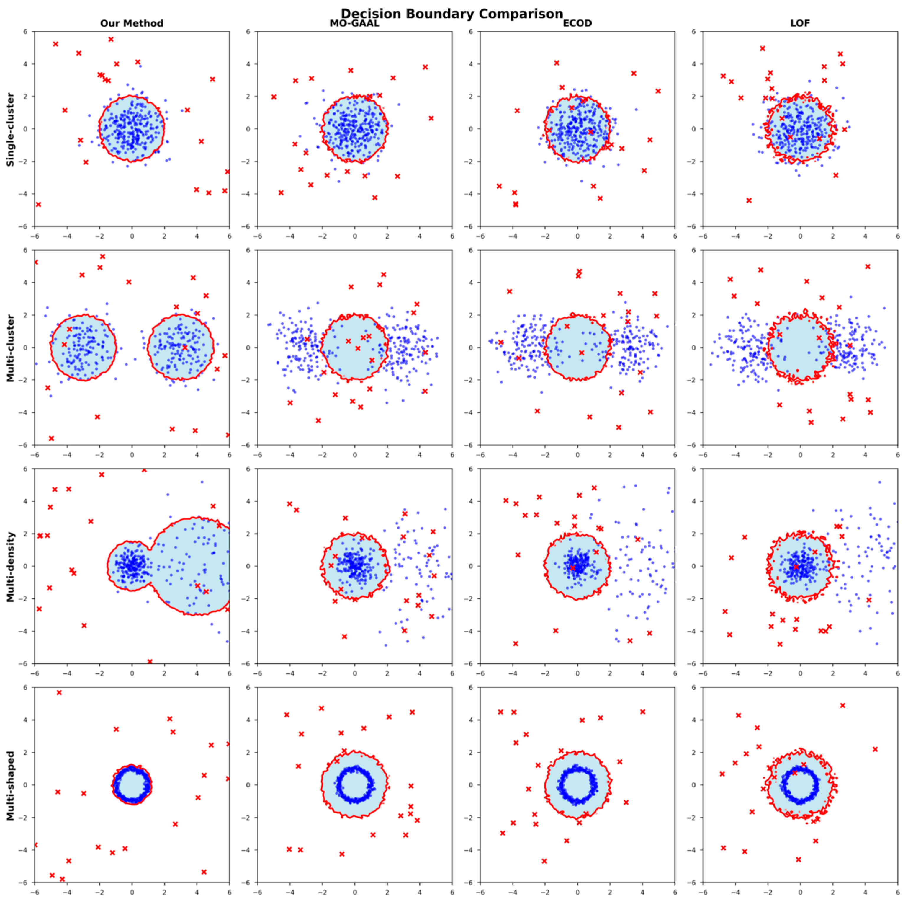
To further validate the superior performance of the proposed ADAEN method in handling different data distribution scenarios, particularly its adaptability in complex data structures and multi-modal distributions, we designed decision boundary visualization experiments based on synthetic datasets. We used scikit-learn library to generate four synthetic two-dimensional datasets, each containing 1000 samples. The four datasets separately simulate single-cluster, multi-cluster, multi-density, and complex geometric shape distribution scenarios. Figure 10’s visualization results clearly demonstrate that this method can generate more accurate decision boundaries, particularly showing remarkable performance improvements when handling non-uniform and multi-cluster scenario distributions.

Figure 10 shows the decision boundary visualization results of this paper’s ADAEN method and three other representative MO-GAAL [42], ECOD [17], and LOF [40] methods on four different datasets. Through comparative analysis, we can clearly observe the distinctive characteristics of different methods when handling various data distributions. On single-cluster datasets, this paper’s method can form more compact and accurate decision boundaries, effectively encompassing normal data points while maintaining appropriate boundary margins. In contrast, the LOF method’s boundaries are too loose, easily misclassifying anomalous points as normal, while ECOD and MO-GAAL show better performance, but their boundary smoothness and tightness are inferior to this paper’s method.

To elucidate the fundamental reasons behind ADAEN’s superior boundary quality, we analyze the inductive biases and architectural limitations of the competing frameworks from a theoretical perspective. LOF relies on local reachability distances in the raw feature space, making it susceptible to the “curse of dimensionality” and sampling noise, which manifests as jagged, irregular boundaries in Figure 10. MO-GAAL, though adversarially trained, suffers from mode collapse—a common pathology in GAN-based methods where the generator fails to cover multi-modal distributions, which is evident in its inability to separate bimodal clusters. ECOD assumes feature independence, forcing it into axis-aligned rectangular boundaries that cannot capture non-convex topologies like the ring structure. Deep SVDD imposes a unimodal hypersphere assumption, which is inherently incapable of modeling hollow geometries. In contrast, ADAEN addresses these deficiencies through three synergistic mechanisms: (1) the AHFE generator maps data into a learned latent manifold, avoiding raw-space distance concentration; (2) the MSAD discriminator’s multi-scale diffusion enables simultaneous global separation (high-noise regime) and local refinement (low-noise regime); and (3) Transformer-based multi-head attention captures non-linear feature dependencies without positional constraints, enabling precise modeling of complex, non-convex data topologies.

In single-cluster distribution scenarios, the proposed ADAEN method generates ideal circular decision boundaries that tightly encompass normal samples while maintaining appropriate boundary margins. In contrast, MO-GAAL’s boundaries are too loose, with multiple anomalous points mistakenly being included in normal regions; ECOD generates irregular multi-boundary situations with obvious concavities at boundaries; and LOF shows naturally reasonable boundary shapes but has overly circular boundary regions, unable to fully distinguish normal sample distributions.

When facing bimodal distributions, this paper’s ADAEN method successfully identifies and encompasses two independent normal regions, with each having precise elliptical boundary packages. MO-GAAL completely fails to identify bimodal structures, generating single large-scale boundaries; ECOD, although partially identifying bimodal characteristics, has two boundaries existing in severe overlap; and the LOF method divides data space through degrees, generating multiple fragmented small boundaries.

In density difference scenarios, this paper’s ADAEN method demonstrates excellent adaptive capability, generating compact boundaries for dense regions while providing more relaxed boundary packages for low-density regions. MO-GAAL uses unified boundary strategies, resulting in poor detection effectiveness; ECOD shows considerable performance in high-density regions but cannot effectively adapt to low-density distributions; and LOF, due to dependence on local density ratios, generates erroneous judgments in density variation regions.

Ring-shaped distribution serves as the most challenging non-convex shape data, fully validating this paper’s method’s superiority. This paper’s method perfectly learns ring-shaped decision boundaries, accurately identifying central cavity regions as anomalous. MO-GAAL generates boundaries encompassing entire regions, treating central cavity regions as normal and completely ignoring ring-shaped structural characteristics; ECOD generates fragmented irregular boundaries, unable to accurately carve complete ring-shaped structures; and LOF shows considerable recognition of ring-shaped outlines, but decision boundaries exhibit obvious local fluctuations and irregularities, with insufficient boundary smoothness and accuracy.

Therefore, ADAEN maintains stable and superior detection performance across different data distribution patterns and datasets. This superior performance capability stems from adaptive hierarchical feature evolution and multi-scale robust adversarial gradient loss function cooperation. Generation achieves effective mapping to high-dimensional feature representation through an adaptive position awareness mechanism, with third-order feature encoding multi-head self-attention mechanisms, enabling the parallel processing of different feature sub-spaces. Dual-path residual fusion ensures effective combination of deep features and original information. Simultaneously, the multi-scale robust adversarial gradient loss function enables large-scale data through diffusion-conditional Wasserstein loss optimization at multi-noise scales. The gradient penalty mechanism ensures that the discriminator satisfies the Lipschitz continuity conditions, effectively preventing gradient explosion problems during training. Generator optimization loss provides stable gradient signals through a negative Wasserstein distance. The adaptive weighting mechanism dynamically balances gradient loss components according to training status, further enhancing model convergence stability. Generator feature optimization capability complements the discriminator stability optimization mechanisms, enabling generators to gradually learn and generate complex data patterns. This framework design enables ADAEN to demonstrate outstanding adaptability and robustness across different-dimensional datasets.

Regarding computational overhead, ADAEN makes certain trade-offs for higher accuracy compared to other methods (see

Table 3. Comparison of training and inference time under unified hardware settings.

Method	Training Time per Dataset (h)	Inference Time per Sample (ms)	Normalized Total Time (h), N = 10,000
Deep SVDD	4.5	52.8	4.6467
MO-GAAL	6.8	38.9	6.9081
Mamba-AD	2.8	18.3	2.8508
DiffusionAD	10.2	55.7	10.3547
ADAEN (Ours)	4.5	25.8	4.5717

). On high-dimensional datasets in Arrhythmia (>100 dims), ADAEN requires 4.5 h for training compared to Mamba-AD’s 2.8 h (+60.7%), and 25.8 ms inference latency versus 18.3 ms (+40.9%). This additional cost stems mainly from the Transformer block (multi-head projections and FFN/residual refinement) used to model complex cross-feature interactions in permutation-invariant tabular data. However, this investment yields substantial returns: a 2.4% AUC improvement (0.842 → 0.862) and a 15.7% reduction in false positive rate. Notably, ADAEN achieves 53.6% faster inference than diffusion-based DiffusionAD (55.7 ms) by leveraging direct discriminator scoring instead of iterative denoising.

Specifically, the normalized total time is computed by summing the per-dataset training time and the inference time required for 10,000 samples, with inference latency being converted from milliseconds to hours for fair comparison across methods.

3.4.2. Performance Metric Comparison

To objectively demonstrate that our proposed ADAEN architecture’s anomaly detection performance surpasses other methods, we conducted comprehensive comparative experiments on 14 UCI benchmark datasets. The comparison methods include traditional statistical-based LOF, deep-learning-based Deep SVDD [41], generative adversarial network-based MO-GAAL, diffusion-model-based DiffusionAD [43], and state-space-model-based Mamba-AD [44]. Experimental results are shown in

Table 4. Comprehensive comparison of anomaly detection performance across different data dimensions. Note: Bold values indicate the best performance. The up arrow (↑) indicates that higher values are better. The down arrow (↓) indicates that lower values are better.

Dimension	Dataset	Methods	Error ↓		Efficiency		Overall Performance ↑
			MAE	MSE	Training (h) ↓	Inference (ms) ↓	Avg AUC	Avg F1
Low (<20)	Pima, Shuttle, Stamps	Deep SVDD [41]	0.142	0.028	2.1	38.5	0.818	0.815
		MO-GAAL [42]	0.125	0.023	3.5	28.7	0.858	0.857
		DiffusionAD [43]	0.098	0.018	6.8	42.3	0.906	0.910
		Mamba-AD [44]	0.095	0.017	1.8	13.5	0.910	0.910
		ADAEN	0.087	0.015	3.2	21.8	0.928	0.928
Medium (20–100)	Waveform, WDBC, Ionosphere	Deep SVDD [41]	0.158	0.035	2.8	45.2	0.803	0.798
		MO-GAAL [42]	0.132	0.028	4.2	33.5	0.877	0.891
		DiffusionAD [43]	0.105	0.021	7.5	48.6	0.908	0.919
		Mamba-AD [44]	0.103	0.020	2.1	15.8	0.912	0.921
		ADAEN	0.092	0.017	3.8	23.2	0.936	0.935
High (>100)	Arrhythmia, HAR, p53Mutant	Deep SVDD [41]	0.215	0.068	4.5	52.8	0.788	0.759
		MO-GAAL [42]	0.178	0.052	6.8	38.9	0.817	0.816
		DiffusionAD [43]	0.145	0.038	10.2	55.7	0.838	0.838
		Mamba-AD [44]	0.142	0.036	2.8	18.3	0.842	0.842
		ADAEN	0.128	0.031	4.5	25.8	0.862	0.862

.

ADAEN effectively bridges the performance gap between traditional methods and deep learning approaches. On low-, medium-, and high-dimensional datasets, Deep SVDD achieved AUC values of 0.818, 0.803, and 0.788, respectively. Our method improved the AUC to 0.928, 0.936, and 0.862, respectively, representing improvements of 13.4%, 16.6%, and 9.4%.

On low-dimensional datasets (<20 dimensions), ADAEN achieved an average AUC and F1-Score of 0.928. The method’s MAE was 0.087 and the MSE was 0.015. Compared to Mamba-ADs 0.095 and 0.017, ADAEN’s MAE decreased by 8.42% and MSE decreased by 11.76%. ADAEN’s AUC and F1 improved by 2.0% compared to Mamba-AD’s 0.910.

On medium-dimensional datasets (20–100 dimensions), ADAEN achieved an AUC of 0.936 and an F1-Score of 0.935. The method’s MAE was 0.092 and the MSE was 0.017. Compared to Mamba-AD’s 0.103 and 0.020, ADAEN’s MAE decreased by 10.68% and the MSE decreased by 15.00%. ADAEN’s AUC improved by 2.6% compared to Mamba-ADs 0.912, and the F1 improved by 1.5% compared to 0.921.

On high-dimensional datasets (>100 dimensions), ADAEN achieved an AUC of 0.862 and an F1-Score of 0.862. The method’s MAE was 0.128 and the MSE was 0.031. Compared to Mamba-AD’s 0.142 and 0.036, ADAEN’s MAE decreased by 9.86% and the MSE decreased by 13.89%. ADAEN’s AUC and F1 both improved by 2.4% compared to Mamba-AD’s 0.842.

ADAEN’s high detection accuracy primarily stems from the innovative design of the multi-scale adaptive diffusion enhancement discriminator. This discriminator dynamically adjusts noise intensity across different diffusion stages through cosine-scheduled adaptive noise injection strategies. This enables the discriminator to preserve critical feature information at multiple scales. Adaptive noise regulation injection deeply couples diffusion step information with data features, endowing the discriminator with diffusion-stage awareness. The dynamic diffusion intensity closed-loop adaptive adjustment dynamically optimizes diffusion parameters based on discriminator performance. This mechanism achieves collaborative evolution between diffusion processes and discriminative training. Experiments show that introducing this discriminator alone can improve AUC by 5.0%, demonstrating the core role of multi-scale diffusion mechanisms in accuracy enhancement.

ADAEN’s stable performance across different dimensional datasets reflects its strong generalization capability. This generalization capability stems from the collaborative design of the adaptive hierarchical feature evolution generator and multi-scale discriminator. The generator captures the multi-granularity feature through third-order feature encoders and dual-path residual fusion mechanisms. The discriminator’s multi-scale diffusion strategy enables the model to flexibly adapt to data distribution characteristics across different dimensions. On low-dimensional (<20 dimensions), medium-dimensional (20–100 dimensions), and high-dimensional (>100 dimensions) datasets, ADAEN achieved AUC values of 0.928, 0.936, and 0.862, respectively. This stable performance across dimensions demonstrates the generalization capability of the architectural design. Although DiffusionAD employs diffusion models, it lacks adaptive feature evolution capability. Mamba-AD is inferior to ADAEN’s multi-head self-attention mechanism in complex pattern recognition. However, it is worth noting that the relative performance improvement on high-dimensional data will decrease as the data dimensionality and imbalance increase.

ADAEN’s robustness in complex data scenarios is primarily attributed to adaptive adjustment mechanisms and robust loss functions. The multi-scale diffusion strategy in the discriminator addresses the limitations of fixed noise methods that cannot adapt to complex data distributions. This enables ADAEN to maintain high-precision detection when handling non-uniform distributions and multi-modal data. Hierarchical compression discriminative decision-making further enhances the discriminator’s feature extraction efficiency and interference-resistance capability. The multi-scale robust adversarial gradient loss function ensures training stability through Wasserstein distance and gradient penalty mechanisms. This loss function effectively prevents gradient explosion and mode collapse problems. Ablation experiments show that on the non-uniformly distributed multi-density dataset, ADAEN’s MAE decreased by 10.68%, demonstrating the method’s robustness advantages.

3.4.3. Ablation Experiments

The effectiveness of the overall framework has been validated in all previous experiments. In the ablation experiment section, we focus on analyzing the independent contributions of each module and comparing the effects of different module combinations, loss function configurations, and diffusion strategies.

(1)

Architectural components and key sub-module ablation experiments

To verify the independent roles and synergistic effects of the adaptive hierarchical feature evolution generator, multi-scale adaptive diffusion enhancement discriminator, and multi-scale robust adversarial gradient loss function, experimental results on the Arrhythmia dataset are shown in

Table 5. Ablation experiment results for different architectural components. Note: Bold values indicate the best performance. The up arrow (↑) indicates that higher values are better. The down arrow (↓) indicates that lower values are better.

Architecture	Parameters (M) ↓	Error ↓				Accuracy ↑
		Abs Rel	Sq Rel	RMSE	RMSElog	AUC	Precision	Recall
Base (Traditional GAN)	28.6	0.158	0.135	0.572	0.208	0.798	0.742	0.728
Base + AHFE	35.2	0.142	0.119	0.528	0.195	0.826	0.771	0.756
Base + MSAD	42.8	0.135	0.108	0.502	0.187	0.838	0.785	0.769
Base + MSAG	28.6	0.149	0.126	0.545	0.201	0.812	0.758	0.743
AHFE + MSAD	45.5	0.118	0.095	0.468	0.175	0.871	0.812	0.798
AHFE + MSAG	35.2	0.133	0.106	0.498	0.185	0.840	0.787	0.772
MSAD + MSAG	42.8	0.125	0.098	0.478	0.179	0.857	0.801	0.786
AHFE + MSAD + MSAG (ours)	48.1	0.109	0.089	0.452	0.168	0.892	0.834	0.821

.

Base represents the baseline model using only traditional GAN architecture, AHFE represents the adaptive hierarchical feature evolution adversarial sample generator, MSAD represents the multi-scale adaptive diffusion enhancement discriminator, and MSAG represents the multi-scale robust adversarial gradient loss function.

From the architectural module ablation experiments, it can be observed that all three core modules make significant contributions to model performance. Compared to the Base model, after independently introducing AHFE (adaptive hierarchical feature evolution adversarial sample generator), the AUC improved from 0.798 to 0.826 (3.5% improvement), and Abs Rel decreased from 0.158 to 0.142 (10.1% reduction), indicating that the adaptive hierarchical feature evolution adversarial sample generator effectively enhanced the model’s ability to capture complex high-order correlations among attributes. After independently introducing the MSAD (multi-scale adaptive diffusion enhancement discriminator), the AUC improved to 0.838 (5.0% improvement), demonstrating that the diffusion mechanism enhanced the model’s multi-scale feature learning capability. Although independently introducing the MSAG (multi-scale robust adversarial gradient loss function) showed relatively smaller improvement (1.8% AUC increase), it contributed significantly to the training stability, reducing training time by approximately 15%.

When combining two modules, performance further improved. The AHFE + MSAD combination achieved an AUC of 0.871, improving by 5.4% and 3.9% compared to using AHFE or MSAD alone, respectively, indicating the complementary effects between the adaptive hierarchical feature evolution adversarial sample generator and multi-scale adaptive diffusion enhancement discriminator. The complete model (AHFE + MSAD + MSAG) demonstrated optimal performance, with an AUC of 0.892, representing an 11.8% improvement over the Base model, and the F1-Score improved from 0.735 to 0.827 (12.5% improvement). Although the parameter count increased from 28.6 M to 48.1 M (68.2% increase), this resulted in significant performance gains, proving the efficiency of the architectural design.

To further verify the necessity of internal technical designs within each architectural component, we systematically removed key sub-modules from the complete model and analyzed their impact on the overall performance. These sub-modules include the following: diffusion module and diffusion step encoding (internal components of MSAD), attribute encoding, multi-head attention, and residual connections (internal components of AHFE). Through this fine-grained ablation analysis, we can gain a deep understanding of each technical detail’s contribution to the final performance. Experimental results are shown in

Table 6. Ablation experiment results for core sub-components.

Configuration	Pima (8 Dims)		SpamBase (57 Dims)		PenDigits (16 Dims)		Arrhythmia (279 Dims)
	AUC	F1-Score	AUC	F1-Score	AUC	F1-Score	AUC	F1-Score
w/o Attribute Encoding	0.815	0.808	0.891	0.885	0.963	0.960	0.862	0.856
w/o Multi-Head Attention	0.821	0.814	0.896	0.890	0.968	0.965	0.868	0.862
w/o Residual Connection	0.832	0.825	0.907	0.902	0.975	0.973	0.878	0.872
w/o Diffusion Module	0.782	0.773	0.856	0.847	0.942	0.938	0.835	0.828
w/o Diffusion Step Encoding	0.803	0.795	0.878	0.871	0.956	0.953	0.851	0.844
Complete Model	0.851	0.844	0.925	0.920	0.987	0.985	0.892	0.887

.

w/o indicates the removal of the corresponding component. Diffusion module, diffusion step encoding, adaptive feature attribute encoding, multi-head attention, and residual connections, respectively, correspond to key technical components in the innovations.

Sub-module ablation experiments validated the importance of each component across four datasets with different characteristics: Pima, SpamBase, PenDigits, and Arrhythmia. After removing the diffusion module, all datasets showed significant performance degradation, with the high-dimensional Arrhythmia dataset’s AUC decreasing from 0.892 to 0.835 (6.4% decline), and the low-dimensional Pima dataset decreasing from 0.851 to 0.782 (8.1% decline), demonstrating the universal effectiveness of the diffusion component across different dimensional data.

Removal of the diffusion step encoding component resulted in an average performance decrease of 4.5%, with particularly pronounced impact on the SpamBase text dataset (5.1% AUC reduction), illustrating the importance of diffusion stage information for the generative diffusion process. Although learnable attribute encoding contributed relatively less (average decline of 3.2%), it still provided a 2.5% performance improvement on the PenDigits image dataset, indicating the auxiliary role of the attribute identity information for distinguishing heterogeneous features. Removal of multi-head attention and residual connection components resulted in average performance decreases of 2.3% and 1.5%, respectively. While the impact was smaller, these components are indispensable for the model’s expressive capability and training stability.

(2)

Loss function ablation experiments

To demonstrate the effectiveness of the proposed multi-scale robust adversarial gradient loss function in improving anomaly detection performance, we conducted ablation studies on Wasserstein adversarial loss, ${\mathcal{L}}_D$, gradient penalty loss, ${\mathcal{L}}_{GP}$, and generator optimization loss, ${\mathcal{L}}_G$, based on the Pima and SpamBase datasets, as shown in

Table 7. Loss function combination ablation experiments. Note: The checkmark (✓) indicates that the corresponding loss component is included.

Method	Loss Function				Pima Dataset				SpamBase Dataset
	L_D	L_GP	L_G	L_AF	AUC	Precision	Recall	F1-Score	AUC	Precision	Recall	F1-Score
No Loss Constraint					0.612	0.585	0.572	0.578	0.698	0.672	0.658	0.665
Only L_D	✓				0.745	0.712	0.698	0.705	0.823	0.795	0.781	0.788
L_D + L_G	✓		✓		0.792	0.758	0.745	0.751	0.865	0.836	0.823	0.829
L_D + L_GP	✓	✓			0.803	0.769	0.756	0.762	0.878	0.849	0.836	0.842
L_D + L_G + L_GP	✓	✓	✓		0.828	0.795	0.782	0.788	0.902	0.872	0.860	0.866
Complete Loss (Ours)	✓	✓	✓	✓	0.851	0.817	0.805	0.811	0.925	0.895	0.883	0.889

.

${\mathcal{L}}_D$ represents the Wasserstein adversarial loss, ${\mathcal{L}}_{GP}$ represents the gradient penalty loss, ${\mathcal{L}}_G$ represents the generator optimization loss, and ${\mathcal{L}}_{AF}$ represents the adaptive feedback adjustment mechanism.

Table 7 provides a detailed demonstration of the roles of the three individual components, ${\mathcal{L}}_D+{\mathcal{L}}_G+{\mathcal{L}}_{GP}$, in the adaptive objective loss function. On the Pima dataset, when no specialized loss function was used, the AUC was only 0.612. After introducing the Wasserstein adversarial loss, ${\mathcal{L}}_D$, it improved to 0.745 (21.7% improvement), indicating that the adversarial loss provided the model with a fundamental discriminative learning capability. After adding the generator optimization loss, ${\mathcal{L}}_G$, the AUC further improved to 0.792 (6.3% improvement), showing that negative Wasserstein distance optimization helps to improve generation quality and stabilize training gradients.

The introduction of the gradient penalty loss, ${\mathcal{L}}_{GP}$, significantly improved training stability, with the ${\mathcal{L}}_D+{\mathcal{L}}_{GP}$ combination showing a 7.8% improvement compared to ${\mathcal{L}}_D$ alone. The combination of all three loss functions (${\mathcal{L}}_D+{\mathcal{L}}_G+{\mathcal{L}}_{GP}$) achieved an AUC of 0.828, approaching the performance of the complete model.

Similar trends were observed on the SpamBase dataset, where the complete loss function showed a 32.5% AUC improvement compared to the unconstrained case (from 0.698 to 0.925), demonstrating the universality of the loss function design across different data types.

(3)

Diffusion strategy ablation experiments

To demonstrate the superiority of the cosine scheduling diffusion strategy, we conducted experiments on the PenDigits dataset to examine the impact of different scheduling strategies on the model performance. The noise scheduling strategy during the diffusion process directly affects the training effectiveness and anomaly detection performance. The experimental results are shown in

Table 8. Comparison of different diffusion scheduling strategies. Note: The up arrow (↑) indicates that higher values are better. The down arrow (↓) indicates that lower values are better.

Diffusion Strategy	AUC ↑	Precision ↑	Recall ↑	F1-Score ↑	MAE (h) ↓	MSE ↓
No Diffusion	0.942	0.925	0.918	0.921	2.1	285
Linear Scheduling	0.968	0.952	0.945	0.948	3.2	245
Quadratic Scheduling	0.973	0.957	0.951	0.954	3.5	230
Sigmoid Scheduling	0.978	0.963	0.956	0.959	3.8	225
Cosine Scheduling (Ours)	0.987	0.972	0.966	0.969	3.6	210

.

The diffusion strategy experiments demonstrate that the cosine scheduling strategy adopted in this paper achieved optimal performance (AUC = 0.987), representing a 1.96% improvement over linear scheduling. Cosine scheduling increases noise slowly in low-noise regimes, preserving more original features, while rapidly increasing noise in later stages to generate diverse samples. The experimental training time of 3.6 h falls within a reasonable range and achieved the fastest convergence (210 epochs). This diffusion strategy realizes the optimal balance between performance and efficiency.

To validate the necessity of the “Adaptive” mechanism, we compared the proposed method against three fixed strategies: no diffusion, fixed intensity (p = 0.5), and fixed intensity (p = 1.0). As shown in

Table 9. Comparison of different diffusion intensity strategies (Arrhythmia dataset). Note: The up arrow (↑) indicates that higher values are better. The down arrow (↓) indicates that lower values are better.

Diffusion Strategy	Description	AUC ↑	F1-Score ↑	Convergence Epoch ↓
No Diffusion	Baseline (Standard GAN)	0.835	0.828	-
Fixed Intensity (p = 1.0)	Maximum Noise Constant	0.848	0.841	245
Fixed Intensity (p = 0.5)	Moderate Noise Constan	0.872	0.865	210
Adaptive (Ours)	Dynamic Closed-Loop	0.892	0.887	160

, the no diffusion baseline yields the lowest performance (AUC 0.835), confirming the fundamental value of the diffusion module. The fixed p = 1.0 strategy employs maximum noise intensity throughout training, which disrupts the feature’s semantic integrity, resulting in suboptimal performance (AUC 0.848). While the fixed p = 0.5 strategy achieves respectable results (AUC 0.872), it fails to adapt to the changing difficulty of the discriminator during training. In contrast, our adaptive (closed-loop) strategy dynamically adjusts p based on the discriminator’s dynamic training feedback. This not only achieves the highest detection accuracy (AUC 0.892) but also accelerates convergence, reaching equilibrium 50 epochs earlier (Epoch 160) compared to the fixed strategy (Epoch 210).

4. Conclusions

This paper proposes an adaptive diffusion adversarial evolutionary network (ADAEN), which achieves accurate anomaly detection in tabular data under unlabeled conditions. The method mainly consists of three components: an adaptive hierarchical feature evolution generator, a multi-scale adaptive diffusion enhancement discriminator, and a multi-scale robust adversarial gradient loss function. The adaptive hierarchical feature evolution generator combines adaptive feature attribute encoding and a third-order feature encoder to capture complex feature dependencies at multiple granularities. A dual-path residual fusion mechanism ensures information integrity, thereby improving the model’s generalization ability. The multi-scale adaptive diffusion enhancement discriminator dynamically adjusts the diffusion intensity using a cosine-scheduled noise injection strategy and achieves co-evolution between the diffusion process and discriminative training through a closed-loop feedback mechanism. The multi-scale robust adversarial gradient loss function utilizes Wasserstein distance optimization to distinguish between the distributions of real and generated data and introduces a gradient penalty mechanism to ensure training stability and convergence. Experiments on 14 UCI benchmark datasets demonstrate that the ADAEN model constructed from these three components achieves superior performance compared to the existing state-of-the-art methods.

However, the proposed method has high algorithmic complexity, and further research is needed to reduce computational overhead through lightweight attention structures and model compression techniques. Furthermore, ADAEN performs well and stably on numerous benchmark datasets. However, its relative performance advantage gradually diminishes with increasing data dimensionality and imbalance (as shown in experiments on datasets such as Arrhythmia and p53Mutant). This limitation mainly stems from the increased complexity of high-dimensional feature interactions and the sparsity of outliers in extremely imbalanced cases. Lightweight architecture optimization and imbalance-aware learning strategies are the main approaches to address this problem.

References

1. Xu, H.; Chen, W.; Zhao, N.; Li, Z.; Bu, J.; Li, Z.; Liu, Y.; Zhao, Y.; Pei, D.; Feng, Y.; et al. Deep Isolation Forest for Anomaly Detection. IEEE Trans. Knowl. Data Eng. 2023, 35, 12591–12604. [Google Scholar] [CrossRef]
2. Wuest, M.; Huber, L.G. Fully Unsupervised Anomaly Detection in Industrial Images with Unknown Data Contamination. In Proceedings of the 2025 IEEE Swiss Conference on Data Science (SDS), Zurich, Switzerland, 5–7 June 2025; IEEE: Piscataway, NJ, USA, 2025; pp. 40–47. [Google Scholar]
3. Samariya, D.; Ma, J.; Aryal, S.; Kotagiri, R. Detection and Explanation of Anomalies in Healthcare Data. Health Inf. Sci. Syst. 2023, 11, 22. [Google Scholar] [CrossRef] [PubMed]
4. Xia, H.; An, W.; Zhang, Z. Credit Risk Models for Financial Fraud Detection: A New Outlier Feature Analysis Method of XGBoost With SMOTE. J. Database Manag. 2023, 34, 1–19. [Google Scholar] [CrossRef]
5. Domanska, O.; Martsyshyn, V.; Buhrii, O. Density-Based Outlier Detection: Supervised Approach Based on Virtual Points. In Proceedings of the 2023 IEEE 13th International Conference on Electronics and Information Technologies (ELIT), Lviv, Ukraine, 26–28 September 2023; IEEE: Piscataway, NJ, USA, 2023; pp. 97–101. [Google Scholar]
6. Rahmati, F.; Gharaei, R.H.; Nezamabadi-Pour, H. ARDOD: Adaptive Radius Density-Based Outlier Detection. Evol. Intell. 2024, 17, 2847–2863. [Google Scholar] [CrossRef]
7. Yılmaz, A.; Das, R. A Novel Hybrid Approach Combining GCN and GAT for Effective Anomaly Detection from Firewall Logs in Campus Networks. Comput. Netw. 2025, 259, 111082. [Google Scholar] [CrossRef]
8. He, Y.; Yang, B.; Jin, W.; Zhang, X.; Li, X. A Parallel Neural Network Based Structural Anomaly Detection: Leveraging Time-Frequency Domain Features. Neurocomputing 2025, 634, 129907. [Google Scholar] [CrossRef]
9. Bae, J.; Park, H.; Chung, M.; Kim, Y. Signed Graph Laplacian for Semi-Supervised Anomaly Detection. In Proceedings of the 2024 International Conference on Artificial Intelligence in Information and Communication (ICAIIC), Osaka, Japan, 19–22 February 2024; IEEE: Piscataway, NJ, USA, 2024; pp. 102–107. [Google Scholar]
10. Kim, B.; Kim, I.; Kim, N.; Park, C.; Oh, R.; Gwak, J. SeMA-UNet: A Semi-Supervised Learning with Multimodal Approach of UNet for Effective Segmentation of Key Components in Railway Images. J. Electr. Eng. Technol. 2024, 19, 3317–3330. [Google Scholar] [CrossRef]
11. Lee, C.H.; Lee, K. Semi-Supervised Anomaly Detection Algorithm Based on KL Divergence (SAD-KL). Proc. SPIE 2023, 12531, 125310M. [Google Scholar] [CrossRef]
12. Mohsenia, N.; Nematzadeh, H.; Akbari, E.; Ghalehsefidi, Z.M. Outlier Detection in Test Samples Using Standard Deviation and Unsupervised Training Set Selection. Int. J. Eng. 2023, 36, 119–129. [Google Scholar] [CrossRef]
13. Nijhuis, M.; van Lelyveld, I. Outlier Detection with Reinforcement Learning for Costly to Verify Data. Entropy 2023, 25, 842. [Google Scholar] [CrossRef]
14. Li, Z.; Wei, S.; Liu, S. Outlier Detection Using Conditional Information Entropy and Rough Set Theory. J. Intell. Fuzzy Syst. 2024, 46, 1899–1918. [Google Scholar] [CrossRef]
15. Bolboaca, R.; Genge, B. Unsupervised Outlier Detection in Continuous Nonlinear Systems: Hybrid Approaches with Autoencoders and One-Class SVMs. In Proceedings of the 17th International Conference on Interdisciplinarity in Engineering (INTER-ENG 2023), Targu Mures, Romania, 5–6 October 2023; Springer: Cham, Switzerland, 2024; Volume 929, pp. 376–398. [Google Scholar]
16. Du, X.; Chen, J.; Yu, J.; Luo, X.; Qian, H. Generative Adversarial Nets for Unsupervised Outlier Detection. Expert Syst. Appl. 2024, 236, 121161. [Google Scholar] [CrossRef]
17. Li, Z.; Zhao, Y.; Hu, X.Y.; Botta, N.; Ionescu, C.; Chen, H.G. ECOD: Unsupervised Outlier Detection Using Empirical Cumulative Distribution Functions. IEEE Trans. Knowl. Data Eng. 2023, 35, 12181–12193. [Google Scholar] [CrossRef]
18. Huyan, N.; Quan, D.; Zhang, X.; Liang, X.; Chanussot, J.; Jiao, L. Unsupervised Outlier Detection Using Memory and Contrastive Learning. IEEE Trans. Image Process. 2022, 31, 6440–6454. [Google Scholar] [CrossRef]
19. Huang, Y.H.; Liu, W.F.; Li, S.; Wang, J.C. Interpretable Single-Dimension Outlier Detection (ISOD): An Unsupervised Outlier Detection Method Based on Quantiles and Skewness Coefficients. Appl. Sci. 2024, 14, 136. [Google Scholar] [CrossRef]
20. Zhou, Y.; Xia, H.; Yu, D.H.; Chen, J. Outlier Detection Method Based on High-Density Iteration. Inf. Sci. 2024, 662, 120286. [Google Scholar] [CrossRef]
21. Schlieper, P.; Luft, H.; Klede, K.; Kister, A.; Hofmann, R. Enhancing Unsupervised Outlier Model Selection: A Study on IREOS Algorithms. ACM Trans. Knowl. Discov. Data 2024, 18, 178. [Google Scholar] [CrossRef]
22. Gao, Y.; Lin, Q.Q.; Ye, S.; Huang, J.; Wen, J.G. Outlier Detection in Temporal and Spatial Sequences via Correlation Analysis Based on Graph Neural Networks. Displays 2024, 84, 102760. [Google Scholar] [CrossRef]
23. Zhao, J.; He, J.; Song, H.; Li, S.; Yang, X. FBOD: An Outlier Detection Algorithm Based on Data Features Suitable for Processing Large-Scale Datasets on Distributed Platforms. In Proceedings of the 2024 10th International Symposium on System Security, Safety, and Reliability (ISSSR), Wuhan, China, 21–23 November 2024; IEEE: Piscataway, NJ, USA, 2024; pp. 267–276. [Google Scholar]
24. Huang, Y.H.; Liu, W.F.; Li, S.; Wang, J.C. A Novel Unsupervised Outlier Detection Algorithm Based on Mutual Information and Reduced Spectral Clustering. Electronics 2023, 12, 4864. [Google Scholar] [CrossRef]
25. Dong, H.; Wang, Q.G.; Ding, W. Chain-Based Outlier Detection for Complex Data Scenarios. In Proceedings of the 2023 IEEE International Conference on Big Data (BigData), Sorrento, Italy, 15–18 December 2023; IEEE: Piscataway, NJ, USA, 2023; pp. 504–509. [Google Scholar]
26. Gao, Q.; Gao, Q.Q.; Xiong, Z.Y.; Tang, B.W.; Zhang, Q. A Double-Weighted Outlier Detection Algorithm Considering the Neighborhood Orientation Distribution of Data Objects. Appl. Intell. 2023, 53, 21961–21983. [Google Scholar] [CrossRef]
27. Mayanglambam, S.D.; Pamula, R.; Horng, S.J. Clustering-Based Outlier Detection Technique Using PSO-KNN. J. Appl. Sci. Eng. 2023, 26, 1703–1721. [Google Scholar] [CrossRef]
28. Huang, J.L.; Cheng, D.D.; Zhang, S.L. A Novel Outlier Detecting Algorithm Based on the Outlier Turning Points. Expert Syst. Appl. 2023, 231, 120799. [Google Scholar] [CrossRef]
29. Chen, B.Y.; Li, Y.X.; Peng, D.Z.; Liu, L.Q.; Zhao, H. Fusing Multi-Scale Fuzzy Information to Detect Outliers. Inf. Fusion 2024, 103, 102133. [Google Scholar] [CrossRef]
30. Li, J.L.; Liu, Z.F. Attribute-Weighted Outlier Detection for Mixed Data Based on Parallel Mutual Information. Expert Syst. Appl. 2024, 236, 121304. [Google Scholar] [CrossRef]
31. Xia, H.; Zhou, Y.; Li, J.G.; Chen, J. Outlier Detection Method Based on Improved DPC Algorithm and Centrifugal Factor. Inf. Sci. 2024, 682, 121255. [Google Scholar] [CrossRef]
32. Ding, C.; Pang, G. Zero-Shot Out-of-Distribution Detection with Outlier Label Exposure. In Proceedings of the 2024 International Joint Conference on Neural Networks (IJCNN), Yokohama, Japan, 30 June–5 July 2024; IEEE: Piscataway, NJ, USA, 2024; pp. 1–8. [Google Scholar]
33. Khan, M.; Tran, P.N.; Pham, N.T.; El Saddik, A.; Othmani, A. MemoCMT: Multimodal emotion recognition using cross-modal transformer-based feature fusion. Sci. Rep. 2025, 15, 5473. [Google Scholar] [CrossRef] [PubMed]
34. Livernoche, V.; Jain, V.; Hezaveh, Y.; Ravanbakhsh, S. On Diffusion Modeling for Anomaly Detection. In Proceedings of the Twelfth International Conference on Learning Representations (ICLR), Vienna, Austria, 7–11 May 2024. [Google Scholar]
35. Thimonier, H.; Popineau, F.; Rimmel, A.; Doan, B.L. Beyond Individual Input for Deep Anomaly Detection on Tabular Data. In Proceedings of the 41st International Conference on Machine Learning (ICML), Vienna, Austria, 21–27 July 2024; ACM: New York, NY, USA, 2024; pp. 48107–48126. [Google Scholar]
36. Sattarov, T.; Schreyer, M.; Borth, D. Diffusion-Scheduled Denoising Autoencoders for Anomaly Detection in Tabular Data. In Proceedings of the 31st ACM SIGKDD Conference on Knowledge Discovery and Data Mining (KDD), Toronto, ON, Canada, 3–7 August 2025. [Google Scholar]
37. Khan, M.; Gueaieb, W.; El Saddik, A.; Kwon, S. MSER: Multimodal speech emotion recognition using cross-attention with deep fusion. Expert Syst. Appl. 2024, 245, 122946. [Google Scholar] [CrossRef]
38. Mustaqeem, K.; El Saddik, A.; Alotaibi, F.S.; Pham, N.T. AAD-Net: Advanced end-to-end signal processing system for human emotion detection & recognition using attention-based deep echo state network. Knowl.-Based Syst. 2023, 270, 110525. [Google Scholar]
39. Han, S.; Hu, X.; Huang, H.; Jiang, M.; Zhao, Y. ADBench: Anomaly Detection Benchmark. In Advances in Neural Information Processing Systems 35 (NeurIPS 2022); Curran Associates, Inc.: Red Hook, NY, USA, 2022; Volume 35, pp. 32142–32159. [Google Scholar]
40. Breunig, M.M.; Kriegel, H.-P.; Ng, R.T.; Sander, J. LOF: Identifying Density-Based Local Outliers. In Proceedings of the 2000 ACM SIGMOD International Conference on Management of Data, Dallas, TX, USA, 15–18 May 2000; ACM: New York, NY, USA, 2000; pp. 93–104. [Google Scholar]
41. Ruff, L.; Görnitz, N.; Deecke, L.; Siddiqui, S.A.; Vandermeulen, R.A.; Binder, A.; Müller, E.; Kloft, M. Deep One-Class Classification. In Proceedings of the 35th International Conference on Machine Learning (ICML), Stockholm, Sweden, 10–15 July 2018; PMLR: New York, NY, USA, 2018; Volume 80, pp. 4393–4402. [Google Scholar]
42. Liu, Y.; Li, Z.; Zhou, C.; Jiang, Y.; Sun, J.; Wang, M.; He, X. Generative Adversarial Active Learning for Unsupervised Outlier Detection. IEEE Trans. Knowl. Data Eng. 2020, 32, 1517–1528. [Google Scholar] [CrossRef]
43. Zhang, H.; Wang, Z.; Wu, Z.; Jiang, Y.G. DiffusionAD: Norm-Guided One-Step Denoising Diffusion for Anomaly Detection. IEEE Trans. Pattern Anal. Mach. Intell. 2025, 47, 7140–7152. [Google Scholar] [CrossRef]
44. He, H.; Bai, Y.; Zhang, J.; He, Q.; Chen, H.; Gan, Z.; Wang, C.; Li, X.; Tian, G.; Xie, L. MambaAD: Exploring State Space Models for Multi-class Unsupervised Anomaly Detection. In Proceedings of the 38th Annual Conference on Neural Information Processing Systems (NeurIPS), Vancouver, BC, Canada, 10–15 December 2024. [Google Scholar]
Figure 1. Adaptive diffusion adversarial evolution network framework.
Asi 09 00036 g001
Figure 2. Adaptive hierarchical feature evolution adversarial sample generator.
Asi 09 00036 g002
Figure 3. Adaptive attribute-aware high-dimensional feature representation.
Asi 09 00036 g003
Figure 4. Single-order feature encoder structure.
Asi 09 00036 g004
Figure 5. Multi-scale adaptive diffusion enhancement discriminator.
Asi 09 00036 g005
Figure 6. Adaptive noise regulation injection.
Asi 09 00036 g006
Figure 7. Diffusion-conditional feature fusion perception.
Asi 09 00036 g007
Figure 8. Hierarchical compression discriminative strategy.
Asi 09 00036 g008
Figure 9. Dynamic diffusion intensity closed-loop adaptive adjustment.
Asi 09 00036 g009
Figure 10. Decision boundary comparison of different methods. Blue dots represent normal samples. Red crosses indicate anomalies. The red lines denote the learned decision boundaries.
Asi 09 00036 g010