Article

Innovative Method for Detecting Malware by Analysing API Request Sequences Based on a Hybrid Recurrent Neural Network for Applied Forensic Auditing

by
Serhii Vladov
1,2,*,
Victoria Vysotska
2,3,
Vitalii Varlakhov
4,
Mariia Nazarkevych
2,*,
Serhii Bolvinov
5 and
Volodymyr Piadyshev
6
1
Department of Scientific Activity Organization, Kharkiv National University of Internal Affairs, 27, L. Landau Avenue, 61080 Kharkiv, Ukraine
2
Department of Combating Cybercrime, Kharkiv National University of Internal Affairs, 27, L. Landau Avenue, 61080 Kharkiv, Ukraine
3
Information Systems and Networks Department, Lviv Polytechnic National University, 12, Bandera Street, 79013 Lviv, Ukraine
4
Engineering and Technical Research Laboratory, National Scientific Centre Hon. Prof. M. S. Bokarius Forensic Science Institute, 8-A, Zolochivska Street, 61177 Kharkiv, Ukraine
5
Department of Organization of Educational and Scientific Training (Doctoral and Postgraduate Studies), Kharkiv National University of Internal Affairs, 27, L. Landau Avenue, 61080 Kharkiv, Ukraine
6
Department of Criminal Analysis and Information Technologies, Odesa State University of Internal Affairs, 1, Uspenska Street, 65014 Odesa, Ukraine
*
Authors to whom correspondence should be addressed.
Appl. Syst. Innov. 2025, 8(5), 156; https://doi.org/10.3390/asi8050156
Submission received: 3 September 2025 / Revised: 3 October 2025 / Accepted: 9 October 2025 / Published: 21 October 2025

Abstract

This article develops a method for detecting malware based on the multi-scale recurrent architecture (time-aware multi-scale LSTM) with salience gating, multi-headed attention, and a sequential statistical change detector (CUSUM) integration. The research aim is to create an algorithm capable of effectively detecting malicious activities in behavioural data streams of executable files with minimal delay and ensuring interpretability of the results for subsequent use in forensic audit and cyber defence systems. To implement the task, deep learning methods (training LSTM models with dynamic consideration of time intervals and adaptive attention mechanisms) and sequence statistical analysis (CUSUM, Kulback–Leibler divergence, and Wasserstein distances), as well as regularisation approaches to improve the model stability and explainability, were used. Experimental evaluation demonstrates the proposed approaches’ high efficiency, with the neural network model achieving competitive indicators of accuracy, recall, and classification balance with a low level of false positives and an acceptable detection delay. Attention and salience profile analysis confirmed the possibility of interpreting signals and early detection of abnormal events, which reduces the experts’ workload and reduces the number of false positives. This study introduces the new hybrid architecture development that combines the advantages of recurrent and statistical methods, the theoretical properties formalisation of gated cells for long-term memory, and the proposal of a practical approach to the model solutions’ explainability. The developed method implementation, implemented in the specialised software product form, is shown in a forensic audit.

1. Introduction and Related Works

Malware has been evolving continuously since personal computers became widespread. Over the decades, many different families and varieties of malware have emerged, causing damage on a wide range of platforms. As attacks become more sophisticated, the damage increases in scale and severity, highlighting the need for modern and effective detection methods [1].
In this regard, approaches to detect malware based on machine learning and artificial neural networks have become much more active in recent years. Research traditionally distinguishes two basic areas of analysis, namely, the software behaviour and static and dynamic analysis [2]. Modern research increasingly uses combined (hybrid) methods that combine the advantages of the static and dynamic approaches, as well as behavioural methods and heuristics, to improve detection accuracy [3]. The main difficulties that require further study are obfuscation and polymorphism of samples, lack of high-quality labelled data, and model vulnerability to adversarial techniques, which makes research in the models’ robustness and data augmentation methods a promising field [4].
In [5], the authors, using data extracted from executable files using the IDA Pro disassembler, implemented a classifier that categorises samples into malicious and safe. In parallel, they applied a dynamic approach—API call sequences analysis—to recognise the running applications’ behaviour and confirm the decision on maliciousness. The study illustrates the practical feasibility of the proposed techniques and emphasises their relevance in detection tasks.
In [6], researchers generated signatures of malicious samples based on Windows API calls and then used these signatures to identify and classify malware. The authors report an accuracy of about 75–80% in recognising the family for each sample type. However, the method remains vulnerable: attackers can change the call sequences or resort to obfuscation, which reduces the signature-based approach’s reliability.
The study [7] offers a different view: directly analysing, instead, the properties of the samples themselves, detection is based on anomalies in the system itself under standard conditions of behaviour. That is, the detector looks for the operational systems’ and applications’ unusual reactions (e.g., registry changes, non-standard network activities), assuming that such effects will manifest even in polymorphic and metamorphic samples. This approach allows us to catch advanced samples that hide their static features.
In [8], the efficiency of the “visualisation using a CNN neural network” approach was demonstrated: API call sequences and other signatures were transformed into images according to specified colour encoding rules, after which convolutional neural networks were used for classification. The experiments showed high accuracy (>90%) on the selected datasets, which confirms the potential of the application behaviour visual representations.
In addition, the following are currently being actively studied:
  • Hybrid methods combining static and dynamic analysis [9,10].
  • Representing sequence methods (call n-grams [11], call diagram representations [12], and API embeddings [13]).
  • Decision trees and boosting application on carefully constructed features [14,15].
  • Preliminary training methods are the self-supervised [16] and contrastive approaches [17] for working with a small amount of labelling.
  • Methods of increasing the models’ resistance to adversarial attacks and obfuscation [18,19].
Thus, Table 1 presents the existing research review results in the subject area and highlights the main shortcomings of existing approaches.
Table 1 analysis reveals a persistent gap in the number:
  • Most methods (static signatures, n-grams, visualisations) are vulnerable to obfuscation and polymorphism, which calls into question their long-term applicability.
  • Existing models cope poorly with very long and sparse sequences of API calls and do not provide stable long-term dependency preservation necessary for recognising deferred or conditional actions of malicious code.
  • Research rarely offers mature mechanisms for the multimodal signals’ efficient fusion (static features, dynamics, network traffic, telemetry), so models lose information content when channels are partially available.
  • There are high-quality labelled and balanced datasets, acute shortages, unified benchmarks, and reproducible evaluation protocols, which hinder objective comparative analysis.
  • Robustness enhancement methods (adversarial training) either worsen overall accuracy or require expensive generation of attack examples.
  • Practical applicability is limited by the predictions’ interpretability problems, high computational cost, and difficulties of deployment in resource-constrained environments.
The identified unresolved issues and gaps in existing research justify the need to develop more robust, multi-temporal, and interpretable architectures (e.g., multi-branch recurrent neural networks with attention mechanisms and pretraining) capable of solving the listed problems simultaneously.

2. Materials and Methods

2.1. Developing a Mathematical Framework for Malware Detection

The study [8] developed one of the approaches to the malicious executable files’ static analysis using convolutional neural networks. This study will consider a method for dynamic analysis of executable modules based on their behavioural features. Such features can be Windows API call sequences, registry read and write operations, or network traffic generated by programme activity. This study focuses on the API call analysis performed by applications in the Windows operating system. Software components access system interfaces (APIs) to implement their functions, and these calls reflect the nature of the application. Therefore, methods based on the API calls analysis are widely used in dynamic software research.
In this case, it is assumed that the API calls alphabet is represented as
A = a 1 , a A .
Then the programme behaviour is represented as a time sequence of pairs (event, time):
S = a i k , t k k = 1 N ,   t 1 < t 2 < < t N ,
where aik A is the API call type (individual types of API calls (a finite alphabet of symbolic tokens), i.e., discrete events, and system or library function names that an application calls at runtime, with the practical choice of alphabet size being determined by the data corpus and the tradeoff between information density and sparsity or complexity), and tk ∈ ℝ+ is the event moment. Additionally, each record can carry labels (call arguments, PID, and network packet size [9,10,11,14,19]). Let the general feature space for an event be denoted as X , then a separate event corresponds to xk X . It is noted that the set S is interpreted as a discrete finite set of hidden states (behaviour modes) in an HMM-type model. Each sS is a categorical label of a behavioural mode responsible for generating observed pairs (ak, tk). Suppose S is realised through a transition matrix. In this case, this matrix has the dimension |S| × |S|, when representing one-hot states, it is a vector of length |S|, and when using embeddings, it is a matrix of magnitude |S| × m, where m is the embedding dimension.
Commentary on Equation (2). If the matrix under consideration is the transition matrix of a hidden Markov model, then its dimension is |S| × |S| (elements are real non-negative numbers (probabilities), rows are normalised (sum is 1), and when using the embedding matrix E, its size is |V| × m (in this study |V| ≈ 587, m = 128), the elements are real (trainable) parameters) and its number of elements is |S|2. If the state is encoded by a one-hot vector, then this is a vector of length |S| (the number of elements is |S|, of which elements are binary {0,1}). When using state embeddings, the embedding matrix has size |S| × m and contains |S| × m elements, where m is the embedding dimension. The parameter N in (2) is the observed sequence length, i.e., the number of pairs (aik, tk) in a given session (the number of events). (In this study, a typical value of N will be used, which is about 102 N ¯ ≈ 120; but, in general, N is specified individually for each sequence.)
In this case, based on [9,10], a discrete representation of the process is introduced as a pulse signal, that is,
X t = k = 1 N x k · δ t t k ,
where δ is the delta function, and the pair (xk, tk) is a discrete event signal. It is noted that for discrete analysis, simply the sequence x k k = 1 N is used [10]. Elements xk are separate events’ features. In the simplest version, this is the API tokens’ index (in the dataset, the dictionary V ≈ 587, indices 0–588). In practical implementation, this is the trained token embedding concatenation and the arguments projection x k = e m b e d a k ; ψ r k R E + D a r g .
It is known that the API call generation stochastic model describes a programme’s behaviour as a random time sequence of events— x k k = 1 N —from the alphabet A with marked time moments tk. Control over this sequence is usually implemented through three interconnected modelling levels:
  • Markov model of order m, where the next event occurrence’s conditional probability is specified and fixes the finite memory of the system and local context dependencies [20,21,22]. In this case, it is assumed that the event sequence has a Markov dependence of order m:
P r = x k x k 1 , , x k m = P x k h k 1 ,
where hk−1 = (xk−1, …, xkm). For a finite alphabet, the model is given by the conditional probabilities P(x | h).
In Equation (4), the function is given by the conditional probability of the next event given the history P(xk|hk−1), where hk−1 = (xk−1, …, xkm) captures the Markov dependence of order m. Elements xk are individual events from the feature space X , the index API (integer in the range 0–588) with time tk, and the arguments ψ(rk) projection.
Commentary on Equation (4). The conditional events’ probability is defined over a discrete event alphabet X (the API call types set). Formally, a measure P is determined on the σ-algebra of sequences Ω = X * (or on a finite subset of length N), and the conditional probability is considered as a function P(xk|hk−1), where xk X is the next element and hk−1 is the previous m events’ history (context). Probability is considered on the probability space (Ω, F , ℙ), where Ω is the set of all admissible outcomes (for example, all trajectories (ak, tk)), F is the corresponding σ-algebra, and ℙ is the probability. The conditional probability is defined in the traditional way, that is, for ℙ(B) > 0 P A B = P A B P B , which is the discrete or density case, defined in joint densities terms), and in a general measure-theoretical form as a G -measurable random variable ℙ(A | G ) satisfying G P A G d P = P A G for any G ∈ G . The “next” events’ conditional probability, given the history, is defined as P x k h k 1 = P h k 1 , x k P h k 1 , where P(hk−1, xk) is the histories’ joint probability and the subsequent event, and P(hk−1) is the histories’ probability (with P(hk−1) > 0). Since the history has length m, the order dependence must be explicitly stated, so it is proposed to replace hk−1 with h k 1 m = x k 1 , , x k m . And write the conditional probability as P m x k h k 1 m , which eliminates the ambiguity and explicitly captures the models’ memory.
2.
The events (intensity) arrival process, in which events have a time intensity λ(t), and, for example, in the simplest Poisson model:
P N t + Δ t N t = n = i = 1 A Λ i t + t + Δ t n i · exp Λ i t , t + Δ t n i ! , Λ i t , t + Δ t = t t + Δ t λ i s d s .
In the limiting case of small Δt, this gives a single event’s probability of the i-th type: P{one event of the i-th type} = λi(t) · Δt + ot), where λ(t) = (λ1(t), …, λ| A |(t)) is the intensity vector by types.
3.
Hidden Markov models in which a hidden state skS (behaviour mode) is introduced. Then,
P r s k s k 1 = A s k 1 , s k ,   P r x k s k = B s k x k .
Based on the call generation stochastic model, a transition is made to map the sequence into the feature space via the operator Φ, which aggregates the trajectories’ probabilistic and temporal characteristics into a fixed vector z. Mapping the sequence into the feature space (embedding) is the operator:
Φ : N 1 X N R d ,
which transforms an arbitrary time sequence of events x k k = 1 N (where xk X ) into a fixed-size vector:
Φ : x k k = 1 N z R d
In practice, (8) can be represented as a simple frequency vector:
z i = 1 N · k = 1 N 1 x k = a i ,
as an n-grams vector
z i 1 , , i m = 1 N m + 1 · k 1 x k : k + m 1 = a i 1 , , a i m ,
or as a continuous convolution (kernel representation):
z t = 0 t K t , s · x s d s ,
where K is a kernel that preserves the temporal structure (e.g., exponential decay or Gaussian window).
It is noted that (6) introduces a hidden Markov layer, since the observed sequence of events is generated by hidden states skS with a transition matrix and emission distributions defining transitions between behavioural regimes and observation probabilities. Equations (7) and (8) define a mapping operator Φ that transforms an arbitrary time sequence {xk, tk} into a fixed embedding vector z = Φ({xk}), which is a statistical–temporal feature aggregate. Equation (9) is a frequency representation in which the component zi is a simple counter (or proportion) of the occurrence of the i-th token in a session (e.g., a dictionary frequency vector). Equation (10) represents an n-gram model (e.g., a bigram or trigram vector with counters), and Equation (11) represents a continuous convolution or kernel representation, where events are weighted by a kernel over temporal delays (e.g., an exponential decay Kt) = exp(−β · Δ · tK) or a Gaussian window). The component z is computed through a sequence of operations: pretyping and casting T(•), token encoding into an embedding, aggregation (summation, counts averaging for frequencies, n-gram counting, summation, integration with the kernel K for temporal convolution), and normalisation. In practice, features may be concatenated (e.g., token embedding with argument projection), after which the resulting z is used for classification. The transition from (10) to (11) is formally accomplished by replacing the discrete counting statistics of n-grams with its continuous time-smoothed representation, in which, instead of hard counters, an event’s convolution with a kernel function K is introduced, which takes into account ordinal and interval dependencies (the recurring “temporal” weighting function gives a greater contribution to nearby events).
Note 1. It is noted that in Equation (6), the transition matrix A is defined on the state set S × S with non-negative elements and normalised rows j A i j = 1 , and the emission functions Bs are distributions over the feature space X (discrete or continuous). In the time stamps’ presence, it is necessary to explicitly fix X = A × ℝ+ or separately indicate that Bs acts only on the discrete part ak. The embedding operator Φ is correctly defined as Φ : N 1 A × R + N R d (or briefly X + R d ), since the current N 1 X N omits the time component and introduces ambiguity. For (8), it is necessary to explicitly indicate that in the frequency representation z R A and, more strictly, z Δ A 1 . The components are non-negative and summable in (1). In this case, (9) and (10) require the stipulation Nm and note the exponential growth of the dimension of the feature space | A | for unigrams and | A |m for m-grams. The transition from (9) to (10) is explained as a natural generalisation with m = 1 to the total length of an n-gram, and the transition from a discrete n-gram notation to the integral form (11) is justified by introducing the representation of the sequence as a measure x s = k = 1 N e a k · δ s t k , after which the convolution with the kernel yields an equivalent discrete sum z t = k = 1 N K t , t k · e a k (that is, the transition from Equation (10) to (11) is performed by applying the conditional expectation operator or averaging (or the total probability law) over auxiliary variables and/or limiting transition with an integration order exchange, while for correctness it is necessary to stipulate standard technical conditions (integrability, continuity with respect to the parameter, or Markov property), after which (11) follows algebraically from (10)). It is noted that the functions in Equations (6)–(11) are defined either on the set of states S (or on the space of trajectories Ω) or on the index set of time T (for example, ℕ or [0, ∞)). In this case, their values are real numbers ℝ or vector values ℝm, and the probability functions take values in [0, 1]. The initial set is defined as S0S and can be a single point x0 or described by the initial distribution μ0 P (S).
Also significant are the normalisation and type conversion operations T : X X ~ , so that a well-defined embedding is written as Φ(T(x1), …, T(xN)) (this is necessary for heterogeneous features: categorical labels, real-time metrics, and vector arguments must be unified).
When choosing Φ, the ordinal and temporal dependencies’ persistence (to distinguish sequences with the same empirical frequency but with events in a different order), computational complexity, invariances (time shift, scaling), and noise resistance are taken into account. It is noted that in malware detection tasks, a practical requirement is the ability of Φ to preserve long dependent patterns (i.e., to retain rare but informative events).
Note 2. A note on data type correctness for Φ. In practical implementations, input data type mismatches often arise (e.g., mixing categorical labels, real-time metrics, and vector call arguments). Such mismatches should be explicitly recorded and coerced to a single type before applying Φ. Formally, the type correctness requirement is represented as
Φ : S s e q R d ,
where
S s e q N 1 X N ,
and it is necessary that for all k, xk X of one consistent type. An example of incorrectness is
Φ : S s e q R d ,
where “⇸” emphasises that without type matching, the mapping is not well defined. Then the corrective type casting operation T is represented as
Φ T x 1 , , T x N ,   T : X X ~ ,
where X ~ is a unified feature space (e.g., numerical vectors in ℝm).
Once the embedding z = Φ({xk}) is obtained, the transition to class division is performed by modelling the embedding distributions densities for classes ρ0(z) and ρ1(z) for the “safe” H0: benign (harmless programme) and “malicious” H1: malicious (malicious programme) classes, respectively, and applying the likelihood ratio criterion Λ(z) (or equivalent Bayesian or NP tests [23,24]) to make a decision. The optimal Bayesian criterion (with equal penalties) gives a likelihood ratio test of the following form:
Λ z = ρ 1 z ρ 0 z H 0 H 1 η ,
where the prior probabilities and error penalties give the threshold η.
In Equation (16), the test is formulated as a test of two well-defined statistical hypotheses: H0 is the observed embedding, z is generated by the “safe” class distribution with density ρ0(z), and H1 is the z generated by the distribution of the “harmful” class with density ρ1(z). The test statistic is the likelihood ratio Λ z = ρ 1 z ρ 0 z (or the logarithm (z) = logΛ(z)). The decision rule is defined as “Reject hypothesis H0 if Λ(z) > η (equivalent to (z) > log(η)), where the threshold η is chosen in accordance with the required error level according to the Bayes criterion or the Neyman–Pearson rule for a fixed significance level α”. The confidence interval is determined by the fact that in the parametric case, LRT provides an asymptotic criterion for constructing confidence sets of the parameter θ, which is the set of values of θ for which 2 · l θ ^ l θ χ r , 1 α 2 , where r is the number of degrees of freedom (the parameter shift dimension) and θ ^ is the maximum likelihood estimate. Similarly, for the empirical sum of log-ratios S n = k log ρ 1 z k ρ 0 z k , according to the central limit theorem, an approximate 1 − α confidence interval for the mathematical expectation E [(z)] is constructed as l ¯ ± z 1 α 2 · σ ^ l n , where σ ^ l is the sample standard deviation of the log-ratio increments.
Commentary on Equation (16). The null hypothesis H0 is that the observed embedding z is generated by the “safe” classes’ distribution with density ρ0(z), the alternative hypothesis H1 is that z is generated by the distribution of the “harmful” class ρ1(z). The confidence level (significance) is chosen explicitly (usually α = 0.05 is 95% CI; α = 0.10 for 90% or α = 0.01 for 99% are also acceptable). The test statistic of the log-likelihood ratio l z = log Λ z = log ρ 1 z ρ 0 z requires the specification of the limit law: when applying the classical LRT and when regularity is satisfied for parametric models, the statistic 2 · l θ ^ l θ is asymptotically distributed as χ r 2 under H0 (where r is the number of bias parameters), then the threshold is chosen through χ r , 1 α 2 . For the empirical sum of log-ratios S n = k = 1 n l z k , according to the central limit theorem for large n, we have an approximation by the customary law. Therefore, for the mathematical expectation E [(z)], we can construct a 1-α confidence interval of the form l z = log Λ z = log ρ 1 z ρ 0 z . The statistical inference is formulated as follows: according to the Neyman–Pearson rule, reject H0 when Λ(z) > η (or (z) > log(η)), where η is chosen so that P(Λ > η | H0) = α. In parametric LRT, alternatively, reject H0 if 2 · l θ ^ l θ χ r , 1 α 2 , and the confidence interval for the parameter θ is given as a set θ : 2 · l θ ^ l θ χ r , 1 α 2 . For example, for n = 100, sample mean l ¯ = 0.80 and σ ¯ l = 1.20 with α = 0.05, and the obtained 95% CI is [0.80 ± 1.96 ⋅ 1.20 / 10] = [0.5648, 1.0352]. Since the interval lies entirely above zero, this provides sufficient statistical grounds to reject H0 in favour of H1 at the 5% significance level. As an alternative (parametric) example: if for some hypothesis, LRT gave the value 2 · l θ ^ l θ 0 = 6.10 with r = 1, then since χ 1,0.95 2 = 3.84, H0 is also rejected at the 5% level.
According to Neyman–Pearson [24,25], for a fixed false positive rate α, the optimal test is of the LRT type:
Λ z H 0 H 1 c α ,
For online detection, the likelihood ratio logarithm is introduced at each event xk:
l k = log   P r x k H 1 P r x k H 0 .
Then the cumulative log-likelihood is defined as
S n = k = 1 N l k ,
according to which H1 is accepted when SnA, and H1 is rejected when SnB.
CUSUM [26] builds cumulative statistics of the following form:
W n = max 0 , W n 1 + l k ,   W 0 0
and issues a state change signal when Wn exceeds a predetermined threshold h.
From discrete sequential statistics (SPRT, CUSUM) working with individual event log-likelihoods, a proper transition is to describe the embedding x(t) ∈ ℝd evolution as a continuous stochastic process x(t) with a stochastic differential equation of the following form:
d x t = f x t , u t , t d t + G x t , t d W t ,
where u(t) are external influences, W(t) is a multidimensional Wiener (Brown) process [27]. It is noted that Equation (21) is related to the discrete dynamics of a neural network and is expressed through the limit transition as Δt → 0. If the hidden state iteration is defined as x k + 1 = x k + f x k , u k , t k · Δ t + G x k , t k · Δ t · ξ k (where ξk is a random disturbance with zero mean and unit variance), then under standard assumptions (Lipenschitz property of f, G, boundedness of moments, correct noise scaling), the time-interpolated trajectories converge to the stochastic differential equation dx(t) = f(x(t), u(t), t)dt + G(x(t), t)dW(t) solution, where W(t) is the Brownian motion generated by the limit of sums Δ t · ξ k . In this interpretation, x(t) is a continuous latent vector, u(t) is the input, control (e.g., input data or batch statistics), the function f encodes the deterministic part of the update (residual increment), and G · dW models the stochastic component (mini-batch noise, stochastic regularisers, and approximation uncertainty). Then the distribution density p(x, t) satisfies the Fokker–Planck equation [28]:
d p d t = x · f · p + 1 2 · i , j 2 x i x j G · G i , j · p ,
then for classes H0 and H1 we obtain parallel Fokker–Planck equations for densities p0(x, t) and p1(x, t).
For trajectories (taking time into account), measures ℙ0 and ℙ1 are introduced on the trajectory space, and their distinguishability is then quantified using information measures, namely the Kullback–Leibler divergence [29] DKL(ℙ1 ‖ ℙ0), the Fisher information [30] I(θ), the Wasserstein distances Wp, and the total variation dTV, which are related to the error probabilities, the successive criteria convergence rate, and the detector’s overall resolution.
The Kullback–Leibler divergence for measures ℙ0 and ℙ1 on the trajectory space is defined as
D K L P 1 P 0 = E P 1 log d P 1 d P 0 .
Moreover, the higher the DKL value, the easier it is to separate classes.
Fisher information is defined based on the assumption that the density ρ(z; θ) is parameterised by θ:
I θ = E θ log ρ z ; θ 2 .
For the log-likelihood independent increments, a significant deviation probability is subject to estimates of the following form:
Pr P 0 S n > n · γ exp n · I γ ,
where I(•) is the significant deviation theory rate function.
Let us define the distance between the trajectories S (1), S (2) through embeddings:
d S 1 , S 2 = Φ S 1 Φ S 2 2 ,
an alternative to which are the total variational distance dTV(p1, p2) and the Wasserstein distance Wp(p1, p2), defined as
d T V p 1 , p 2 = 1 2 · p 1 x p 2 x d x ,
W p p 1 , p 2 = E .
The distances between trajectories and their clustering estimates define the state space natural metrics and partitions, on which basis the transition to the stochastic process transition operator T and the generator L spectral analysis is carried out, investigating their eigenvalues and eigenfunctions to identify slow modes and stable behavioural patterns. For this, we consider the transition operator (Markov operator) T on L2:
T φ x = E φ x k + 1 x k = x .
Spectral analysis of T (eigenvalues {λi} and eigenfunctions) reveals slow modes of behaviour. An eigenvalue with |λi| ≈ 1 presence indicates stable patterns. The generator L for SDE is
L φ x = f x · φ x + 1 2 · t r G · G · 2 φ x .
In this case, the dynamics x ˙ = f x , t can have different attractors: stable stationary points, limit cycles, and chaotic attractors. The differences between benign and malicious are manifested in the Lyapunov exponents λmax (positive is the sensitivity to initial conditions), as well as in the recurrence indices and stationary distributions. For a stationary point x*, linearisation is performed:
δ x ˙ = J x * · δ x ,   J x f x x
and the minor disturbances’ behaviour is determined by the matrix J(x*) eigenvalues {λi}. The point x* is linearly stable if R (λi) < 0 for all i; it is unstable if R (λi) > 0. For a discrete map xk+1 = F(xk), the stability condition is represented as all eigenvalues of the Jacobian DF(x*) lying inside the unit circle. It is noted that the exponents’ estimate gives a sensitive quantitative measure of the initial condition. The maximum Lyapunov exponent is defined as
λ m a x = lim t 1 t · log δ x t δ x 0 ,
and λmax > 0 indicates an exponential divergence of trajectories (potentially chaotic dynamics), and λmax < 0 indicates disturbances’ exponential decay. In practice, λmax is estimated numerically (Bennettine algorithm [31], etc.) based on the sample. It is noted that the attractor A is an invariant set to which trajectories from the initial conditions of a particular set asymptotically tend. The basin of attraction is defined as
B A = x 0 : lim t dist φ t x 0 , A = 0 .
The attractor types (fixed points, limit cycles, and strange attractors) differ in spectral and statistical characteristics—this is one of the key features for separating classes. Benign systems often have stable stationary (or periodic) attractors, while malicious processes can exhibit multi-attractorism, frequent transitions between regimes, or positive Lyapunov exponents [32,33].
In this case, for stationary dynamics, there exists an invariant measure μ such that if x(0) ∼ μ then the x(t) distribution is constant. Ergodicity means that the temporal averaging is equal to the spatial one:
lim T 1 T · 0 T ϕ x t d t = ϕ x d μ x
for a broad class of observables ϕ. The difference between μ0 and μ1 (classes) is an essential statistical characteristic. For comparison, the distances dTV(μ0, μ1), Wp(μ0, μ1), and the Kullback–Leibler divergence (if densities are available) are used.
In systems with several local minima (attractors), the key indicator is the average exit time (transition) between modes. For stochastic dynamics,
d x = f x d t + ε d W .
In the low-noise asymptotics, the time to exit the no-slip domain is estimated exponentially according to Freidlin–Wentzel:
τ exp Δ S ε ,
where ΔS is the action on the minimum output path. The commutator function q(x) = Pr{first input to B from x} solves the equation for the generator L:
L q x = 0   i n   t h e   d o m a i n ,   q A = 0 ,   q B = 1 .
These values allow us to estimate the mode stability and the switching probability—a distinctive feature of malicious behaviour (for example, frequent transitions). Based on these diagnostic characteristics (Lyapunov exponents, spectral gap, retention times, etc.), the model parameters are trained through the empirical risk minimisation, i.e., the empirical risk optimisation:
R ^ θ = 1 M · i = 1 M l g θ z i , y i + λ · Ω θ ,
where is the loss function (e.g., cross-entropy) and Ω is the regulariser. Then the empirical risk gradient is represented as
θ R ^ θ = 1 M · i = 1 M θ l g θ z i , y i + λ · θ Ω θ .
A necessary condition for a stationary point θ* is a zero gradient, that is,
θ R ^ θ = 0 .
Moreover, if R ^ is convex and C2 is smooth, then this is also a sufficient condition for a global minimum.
Thus, the solution to the minimising empirical risk problem comes down to the suitable numerical method choice (gradient, proximal, or Newtonian [34,35]), the correct regulariser structure consideration, the loss function properties (convexity, smoothness), and hyperparameter control through validation. In particular, the numerical methods and regularisation choice are directly related to the recurrent cells’ internal state dynamics analysis, since it is these decisions that determine the network stability and ability to store information over time [7,36,37,38].
Theorem 1.
On the Long-Term Memory Property of Gated Recurrent Cells.
Consider a recurrent cell class updating the internal state ct ∈ ℝd by the rule ct = gtct−1 + ut, where gt ∈ [0, 1]d is the gate vector (element-wise multiplication), and ut ∈ ℝd is the input. Then, for any sequence of inputs {ut} and gates {gt}, there exist gate values that ensure the information scalar component preservation in the internal state over an arbitrarily large number of steps with an arbitrarily small attenuation. That is, there exists a setting {gt} such that for some i-th component, the initial state c 0 i to c t i contribution remains bounded below by a positive constant as t → ∞.
Proof of Theorem 1.
For a fixed i-th component, a scalar update of the form is specified:
c t = g t c t 1 + u t ,
Unfolding the recursion,
c t i = s = 1 t g s i · c 0 i + k = 1 t s = k + 1 t g s i · u k i ,
where the empty product is equal to 1.
Let g s i = 1 ε s , with small εs ∈ (0, 1). Then,
log s = 1 t g s i = s = 1 t 1 ε s
for small εs. Using the power expansion and a simple estimate of the series tail, for any s, we obtain ε s ε s 2 1 ε s log 1 ε s ε s for 0 < εs < 1 (because log 1 x = k = 1 x k k ). Summing over s = 1, …, t, we obtain strict inequalities s = 1 t ε s s = 1 t ε s 2 1 ε s s = 1 t log 1 ε s s = 1 t ε s . Hence, s = 1 t log g s i = s = 1 t ε s + R t .
If we choose a sequence {εs} such that the series s = 1 ε s < (for example, ε s = ε s 1 + δ , with δ > 0), then the limit
Γ i lim t s = 1 t g s i = exp s = 1 ε s
exists and is positive: 0 < Γ i 1 .
Therefore, the initial state c 0 i contribution is preserved and multiplied by Γ i , which can be made arbitrarily close to 1 by choosing a small parameter ε. As for the inputs’ u k i contribution, it is multiplied by the factors s = k + 1 t g s i . For the chosen εs, these factors do not tend to zero quickly, but if the inputs are bounded and Γ i is close to 1, the initial state contribution will dominate.
Thus, the gate sequence that ensures long-term information preservation about c 0 i is constructively demonstrated. The theorem is proved. □
Thus, Theorem 1 formalises the long-term memory mechanism. The model can store relevant patterns that appeared long ago and use them when making decisions. It is essential for detecting slowly developing attacks or malicious chains of events distributed over time (Appendix A). In practice, this means that it is necessary to include a mechanism for selectively storing significant features (analogous to “gates”) in the architecture so that information about maliciousness indicators that are sparse in time is not lost.

2.2. Development of a Neural Network Model for Detecting Malware

A recurrent neural network based on an LSTM cell is used as a model for classifying programmes by API call sequences. This architecture choice is due to the classical RNNs’ limitations in modelling long-term dependencies [36,37], since LSTM structures are equipped with mechanisms for storing and forgetting information [36,38,39], which allows them to effectively capture and approximate long-term dependencies that arise at arbitrary intervals. This approach is appropriate when analysing events and temporally distributed features, where it is necessary to preserve context over ample time intervals [39,40]. The network is implemented in Python 3.7 using the Keras framework. The constructed recurrent neural network architectural diagram is shown in Figure 1.
As shown in Figure 1, the data passes through an embedding layer that transforms discrete inputs into dense vector representations then through SpatialDropout1D for regularisation and feature correlation reduction. The sequence is processed by an LSTM layer cascade to extract local and medium-term temporal dynamics, after which a time-aware multi-head self-attention block collects the LSTM cells’ output states, takes into account the relative time intervals between events, and adaptively weights each step’s contribution by importance, providing flexible global information aggregation. The attention block output is passed to a dense layer series with dropout to build high-level features, and the final layer produces class probabilities, which together provide malware detection that is sensitive and robust to sparse and long-term behavioural patterns.
For the developed neural network mathematical description, it is assumed that the programme input behavioural sequence is defined as S = a k , t k , r k k = 1 T , ak A (API call type), tk ∈ ℝ+ (moment), tk R (arguments, metrics). The general embedding operator (the mapping function of a sequence into a fixed vector), denoted by Φ, where z = Φ(T(x1), …, T(xN)) is formally the type conversion operation T and kernel representations of time.
At the preprocessing stage in the embedding layer, categorical and real features are first reduced to a single feature space X R m via the operator T. For discrete API indices, a trainable embedding matrix E R A × d c is used:
e k = E a k = E · a k R d c .
The matrix E in Equation (45) is treated as a trainable linear operator, which is a weight matrix that transforms the vector features of an event into a latent (classification) space, that is, E R d z × d a , and it is justified by the need to aggregate and mix the feature’s components to obtain a compact embedding taking into account inter-feature interactions (the E structure can be dense, sparse, or block-like and regularised during training). In this case, ak is not a scalar, but a vector of features a k R d a (for example, a concatenation of the token embedding and the argument’s projections). So the correct notation of the equality is given as z = k E · a k (or, taking into account the bias and nonlinearity, z = σ k E · a k + b , and if the authors had in mind the scalar weights αk with vector features vk, then the correct form will be z = k α k · v k .
If the record contains additional vector attributes rk, we combine
x k = c o n c a t e k , ψ r k R d c .
where ψ(•) is the argument normaliser (projector). It formally corresponds to the operator Φ in the form of a frequency (or kernel) representation or n-gram (or convolution).
The SpatialDropout1D layer is applied across the embedding channels. It specifies a mask m 0,1 d x (the same across time steps) with Pr(mj = 0) = psd, and
x ~ k = m x k .
It is noted that in Equations (46) and (47), the function concat(•) denotes the concatenation operation of feature vectors, i.e., their sequential combination into one longer vector without losing information about each component. For example, if e k R d c and ψ r k R d r , then c o n c a t e k , ψ r k R d c + d r . The algebraic operator ⊙ denotes the element-wise (Hadamard) product of the exact dimensions’ vectors.
The LSTM cell (Figure 2) is a traditional gated LSTM structure with the temporal decay introduction, a salience gate, and an input (memory) kernel temporal modulation to allow the model to controllably retain rare, informative events, reduce the long intervals’ contribution, and ensure the existence theorem of gates for long-term memory (Theorem 1). It is assumed that at the k-th step, its input is x ~ k , the previous hidden state is hk−1 and memory is ck−1, and the time interval is Δtk = tktk−1 (for k = 1, we set Δt1 = 0).
A time core (which can be fixed or trainable) of the following type is introduced:
K τ Δ t = exp α · Δ t ,   α 0 .
or a more general parameterisation of Kτt; θK) (e.g., an exponential and Gaussian mixture), which is consistent with the exponential decay (kernel) ideas.
To isolate rare informative events, a gate sk ∈ [0, 1]d is introduced, calculated as
s k = σ W s · x ~ k + U s · h k 1 + γ s · ϕ x ~ k ,
where ϕ x ~ k is an additional scalar (or vector) “importance score” (e.g., normalised distance to malicious (benign) prototypes or local information score such as Kullback–Leibler divergence), and γs is a coefficient. This gate allows one to enhance the contribution of clearly significant events.
Then, the equations for describing traditional LSTM gates with additional time and salience modulation are given as
i k = σ W i · x ~ k + U i · h k 1 + b i + β i · τ i Δ t k , f k = σ W f · x ~ k + U f · h k 1 + b i + β f · τ f Δ t k , o k = σ W o · x ~ k + U o · h k 1 + b o ,
where τtk) are scalars (vectors) obtained from the time kernel Kτtk) (e.g., τtk) = log(1 + Kτtk)) or the Time2Vec projection [41]), and β*, and γs are the learnable coefficients. It allows the gates to depend on how recent (or distant) the event is.
The candidate for memory update u ~ k is formed as
u ~ k = t a n h W u · x ~ k + U u · h k 1 + b u .
Also introduced is temporal modulation of old memory and salience weighting:
c k = f k K τ Δ t k c k 1 + i k s k u ~ k .
In (52), the first term reduces (in a controlled manner) the old memory contribution for large Δt. Still, due to the theorem of gates for long-term memory (Theorem 1), it is possible to adjust fk ≈ 1 to preserve information when needed.
Then the LSTM cells’ hidden state is defined as
h k = o k t a n h c k .
Comment on long-term memory preservation. Theorem of gates for long-term memory (Theorem 1) guarantees the existence of gate configurations {gt} (here the fk component and/or additional multiplicative factors) for which the initial state contribution does not tend to zero.
After passing through LSTM, a hidden state matrix for the entire sequence is obtained:
H = h 1 , , h T R T × d h .
For multi-head attention, the following type projections are specified:
Q = H · W Q ,   K = H · W K ,   V = H · W V ,
where W Q , W K R d h × d k , W V R d h × d v .
For the scoring time modification, it is assumed that the expression describes traditional scores:
S i j 0 = Q i · K j d k .
A temporary core is introduced in scoring, represented as
S i j = S i j 0 · K τ t i t j ,
after which normalisation is carried out:
A i · = s o f t m a x j S i j C i = j = 1 T A i j · V j .
In the multi-head case, the “heads” are concatenated and projected back. This modification implements the “weighting by time intervals” idea and is consistent with nuclear time representations.
To describe residual connections and normalisation, a standard scheme is used:
C ^ = L a y e r N o r m H + M H A t i m e H , t ,
where M H A t i m e H , t = C 1 , C T gives for each position a weighted representation, where the weights depend not only on the content hi, but also on the time difference ti-tj.
Next, the contexts Ci are aggregated into a fixed-size vector z, for example, via time-weighted pooling:
z = 1 i ω i · i = 1 T ω i · C i ,   ω i = g p o o l t i ,
where g p o o l t i = S i j · exp α · t i t j .
Next, z is passed through a dense layer series with dropout, resulting in logits of the form:
s = M L P z ,   p ^ = s o f t m a x s ,
where p ^ Δ K 1 is the distribution over K classes (usually K = 2: benign and malicious).
Taking into account the trajectory differences, the loss function has the following form:
L C E θ = 1 N · n = 1 N c y n , c · log p ^ n , c , R θ = λ · θ 2 ,   L θ = L C E θ + R θ .
To increase the interclass distance in embedding, a criterion is introduced for the distance between the class embedding distributions (the Kullback–Leibler divergence or the Wasserstein distance analogues), presented in the following form:
L c t r = i , j , k z i z j 2 z i z k 2 + m + .
A regulariser is also added that encourages a significant preservation of memory components for those steps where salience sk is large:
R m e m = μ · k 1 f k K τ Δ t k 1 · I s k > η ,
which penalises strong memory decay if the event is marked as critical. The overall objective function then becomes
L t o t a l = L C E + λ · θ 2 + γ c t r · L c t r + μ · R m e m ,
which is minimised by gradient methods (Adam, RMSprop [42]). The general objective function gradient is
θ L t o t a l = θ L C E + 2 · λ · θ + γ c t r · θ L c t r + μ · θ R m e m ,
in this case, the stationarity is a necessary condition θ L t o t a l θ * = 0 , consistent with the empirical risk minimisation general theory [43].
Table 2 shows a layer-by-layer diagram of the key stages of training the developed neural network (see Figure 1) from preprocessing and tokenisation of input API calls, through embeddings and SpatialDropout, multilayer LSTM branches with subsequent dense blocks and an attention mechanism, to the output classifier, loss function, and optimiser, indicating optional steps (augmentation, adversarial training, and optimisation for deployment).

2.3. Synthesis of a Malware Detection Method for API Request Sequence Analysis

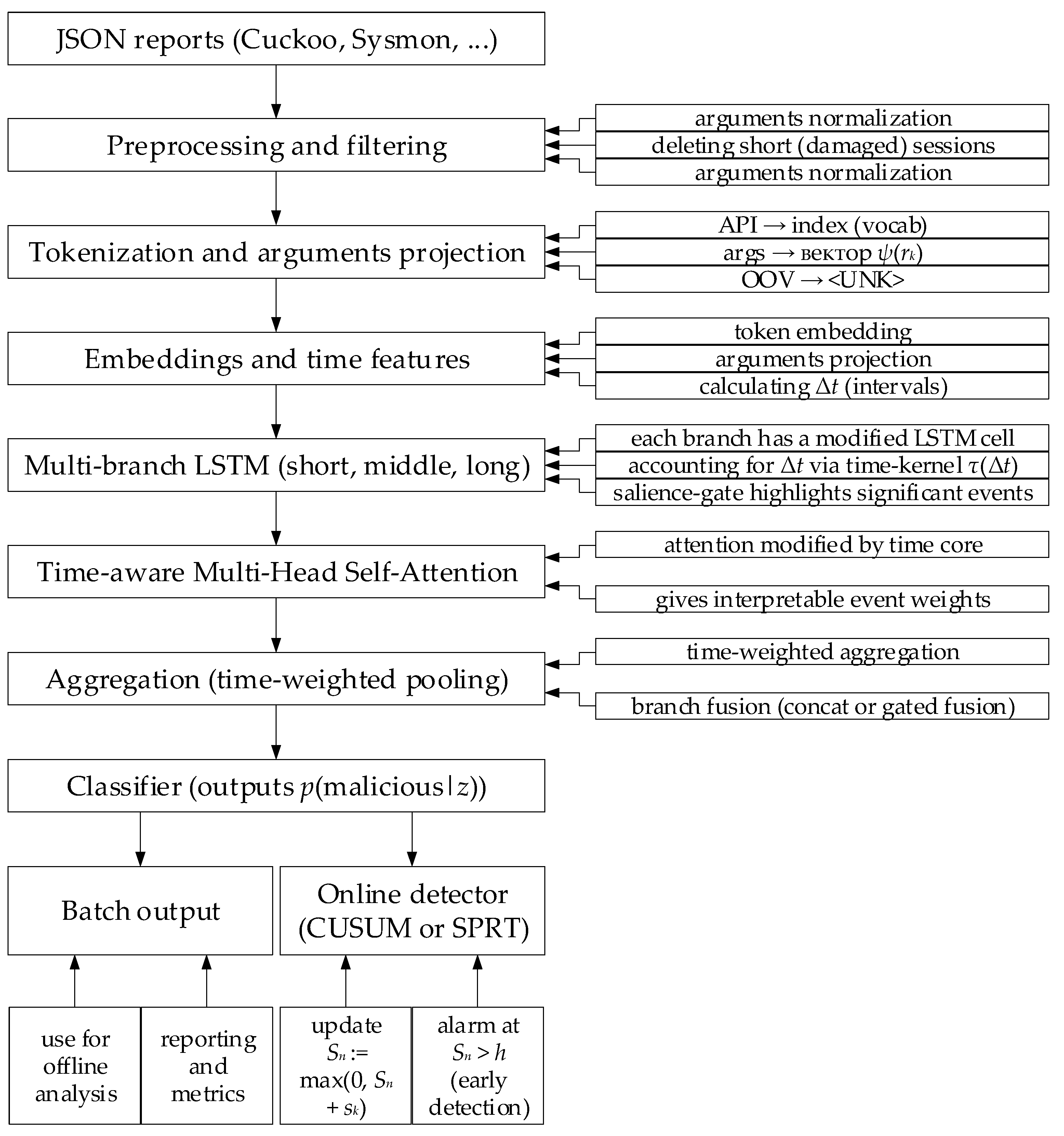
Based on the developed neural network (see Figure 1), a method for detecting malware by analysing sequences of API requests was synthesised, of which the main idea is to transform API event time sequences into stable time-aware embeddings through a modified LSTM branch with salience gates, then make an online (or batch) decision using a neural network classifier combination and sequential criteria (LRT or CUSUM). Figure 3 shows the structural diagram of the developed method. It is noted that the integration of the CUSUM detector into the developed online detection method plays a key role in improving its effectiveness, as it enables prompt monitoring of deviations in incoming data and real-time threat response. The logarithm of the likelihood ratio for the CUSUM statistic is derived from the output probabilities of a neural network, where for each new sequence, the ratio of the probability of an event being benign (H0) to the likelihood of it being malicious (H1) is calculated. This ratio logarithm is then used to update the CUSUM statistic, which analyses the accumulated data and generates alerts about possible anomalies when the statistic value exceeds a predetermined threshold. This hybrid approach, combining the power of deep learning with the precision of statistical methods, enables effective detection of both short-term anomalies and complex long-term attacks, reducing system response latency and minimising false positives.
The system receives Cuckoo JSON reports and extracts sequences of API calls with timestamps and arguments. Each session is filtered (e.g., sequences length ≥ 100), tokenised by the API dictionary, and packaged into length-bucketed batches for efficient training and padding. Timestamps are converted to intervals Δt for subsequent time-aware processing and call arguments are projected into a vector space ψ(rk) and concatenated with token embeddings (type casting operator T and embedding operator Φ).
Tokens are passed through a trainable embedding and SpatialDropout1D. The sequence is then processed by a multi-scale stacked RNN, where each branch is a modified LSTM that takes into account the temporal kernel τt) and introduces an additional salience gating sk (according to Equations (48)–(53)). This design provides a theoretically justified “long-term memory” (see Theorem 1) and allows the modelling of both frequent local patterns and rare but informative events.
The LSTM cells’ outputs are fed to a time-aware multi-head self-attention, where the scoring function is modified by a time kernel Kτt), which makes the attention weights sensitive to the steps’ relative recency according to (56)–(58). It provides interpretability (the attention weights indicate critical steps) and improves the sparse feature extraction. Aggregation is performed according to the scheme “time-weighted pooling → fixed vector z”.
The vector z passes through dense blocks and yields class probabilities p(malicious|z). For batch classification, weighted cross-entropy (including focal or class weights in the imbalance case) and regularisers are used as a penalty for the significant memory components attenuation according to (63) as well as a technique to increase the embeddings interclass distance (the Kullback–Leibler divergence or the Wasserstein distance analogues). For online detection, the log-likelihood ratio Λ(z) and accumulated statistics (SPRT or CUSUM) are additionally calculated. When a new event xk arrives, Sn is updated according to (18)–(20), and an alarm is issued when the threshold h is exceeded, which allows for a quick response to the maliciousness’s early indicators.
Adam performs training with the LR-scheduler, early stopping, and gradient clipping. To combat obfuscation and rare tokens, embedding pretraining (self-supervised or masked), data augmentation of sequences (insertions, deletions, or re-shifts), adversarial training, and stratified sampling or oversampling are used. Monitoring metrics are precision, recall, F1-score, ROC AUC, per-class F1, and specific online metrics such as average detection delay and false alarm rate (FAR) over time.
An experimental sample of the developed method is implemented in the MATLAB Simulink R2014b software environment (Figure 4).
The data source (implemented by the “From Workspace” block) feeds API sequences (indices), timestamps, and arguments. The “Preprocessing” block (implemented by the “Matlab Function” block) filters seq_length ≥ 100, tokenises indices, pads to a window (or batch), calculates Δt = tktk−1, and outputs a project of arguments ψ(rk). Embedding lookup (implemented by the “Matlab Function” block) is a block that stores the embedding matrix (size E = 128). SpatialDropout1D (implemented by the “Matlab Function” block) randomly zeroes embedding channels equally across time-steps. Multi-branch LSTM (implemented by the “Matlab Function” block) extracts multi-scale temporal features. Each branch is a modified LSTM cell with a time kernel τt) and a salience gate sk. “Concatenation” (implemented by the “Concatenate” block) concatenates the branches’ outputs over time. “Time-aware multi-head self-attention” (implemented by the “Matlab Function” block) implements matrix operations Q, K, V, and a scoring matrix S = Q · K T d + t i m e _ b i a s , then softmax and weighted sum. The “Aggregation” block aims to aggregate Context (N × D) into a vector z of size dz. “Dense-blocks and Dropout” (implemented by the “Matlab Function” block) are multiple dense layers, with the last layer giving logits for K classes (K = 2). Dropout can be turned off on inference. The parameters, dense_dropout = 0.3, embedding size, and number of neurons, are configurable. “Softmax” (implemented by the “Matlab Function” block) is a p(malicious|z) classifier. In the “Online Detector (CUSUM)” (implemented by the “Matlab Function” block), the log-likelihood ratio Λ(z) is calculated for each incoming z, and the accumulated statistics Sn or Wn (CUSUM) are updated, and an alarm is generated when the threshold h is exceeded. In the “To Workspace” output block, the results are logged, and an event (trigger) is generated in SIEM.

3. Case Study

3.1. Formation and Pre-Processing of the Input Dataset

The study defines malware as any software or programme code designed with the intentional intent of performing unauthorised or harmful actions against computing systems, data, or their users, including violating the confidentiality, integrity, or availability of resources; providing unauthorised remote access; performing covert data transfer; self-propagation; or sabotage. Key characteristics of malware include the presence of a malicious (hostile) intent, performing actions without the system owner’s informed consent, and the automation of malicious behaviour (e.g., vulnerability exploitation, stealthy persistence, network propagation, encryption, or data exfiltration). A typical example is the WannaCry ransomware worm (May 2017), which exploited a vulnerability in the SMBv1 service (CVE-2017-0144, exploit “EternalBlue”) to self-propagate over the network, downloaded and launched an encryption module, encrypted user files (using a combination of symmetric and asymmetric encryption), left a ransom note, and used TCP/445 network connections for propagation. It demonstrates that malicious behaviour is implemented through characteristic sequences of system calls (process creation, bulk writes, network connections, crypto API calls, etc.), so the Windows API call corpus collected in Cuckoo Sandbox serves as a direct source of observable features for model training.
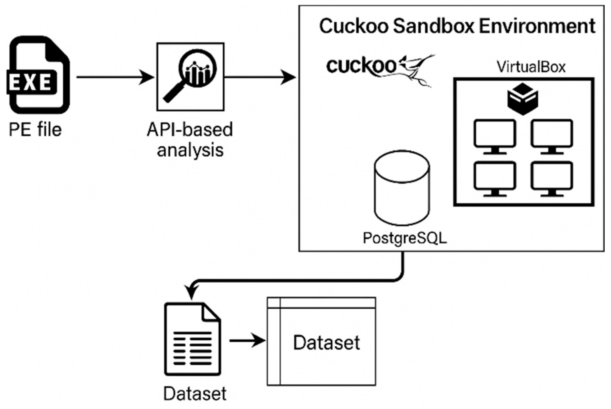
That is why a dataset was obtained for the analysis, including Windows API calls extracted from executable applications. Data was collected using the open and free Cuckoo Sandbox tool, which allows one to run suspicious programmes in a virtualised, isolated environment. During file execution, Cuckoo records the application behaviour and saves the results as JSON reports in the PostgreSQL database. Completed API call records were then extracted from the received reports. The general scheme for preparing the training dataset is shown in Figure 5.
Since the generated set will be used to train the developed neural network, it was filtered. Thus, reports on programme actions containing fewer than 100 API calls were discarded. Further processing consisted of indexing the queries: since 587 different API calls were identified during data collection, these calls were indexed with values from 0 to 588 inclusive. The final data preparation stage for model training was marking the dataset with information about safe and malicious files.
Table 3 provides the input dataset for training description: the fields list (unique sample identifier, benign (malicious) label, API calls indexed sequence and its length, timestamps and call arguments, Cuckoo metadata, and path to the original JSON report), as well as filtering rules (removing records with less than 100 calls) and the 587 unique APIs dictionary details used for tokenisation.
Table 4 presents the training example file_000003 records: the positional call number, the API token corresponding integer index (range 0–588), and the timestamp of each event for the sequences’ first 20 elements (total length seq_length = 312). These data serve as the input representation for training the developed neural network (see Figure 2), where the indices are used as embedding tokens, and the timestamps are used to form time-aware features and masks during padding.
Taking the significance level of α = 0.05 (95%), we use the binomial model for the proportion of successful classifications with a normal approximation according to the central limit theorem as the distribution (for N = 5000 it is sufficient); the observed accuracy was p ^ = 0.964. Then the 95% confidence interval for the accuracy [0.9588, 0.9692] is (95.88–96.92%). Testing the hypothesis H0: p = 0.90 against H1: p > 0.90 gives the statistics z ≈ 15.08 and p-value ≪ 10−10 (extremely small), therefore H0 is rejected, and the model demonstrates a statistically significantly greater accuracy than 90%. As a numerical example of the application of the criteria, it is accepted that at the decision threshold (likelihood or score) η = 0.5, the model gives a malice probability estimate of 0.85, hence the classification “malicious”, and in the accuracy test, the observed p ^ = 0.964 and the indicated CI confirm the practical and statistical reliability of the result.
Table 5 shows the training dataset homogeneity assessment (metrics, their definition, values, and interpretation) for a dataset consisting of N = 5000 samples.
The evaluation shows that the training set is by no means completely homogeneous. While the vocabulary is almost wholly covered (≈96%), there is significant variability in sequence lengths and in the unique token number per sample (high CV and std), as well as strong unevenness in API frequencies (Gini ≈ 0.72) and low average pairwise Jaccard similarity (≈0.11). It means that the model encounters both strongly dominant “frequent” calls and a large number of rare specific API calls, which may lead to problems with overfitting frequent patterns and weak generalisation of rare families. In practice, length bucketing, class weighting (or oversampling), embedding regularisation, sequence data augmentation techniques, and methods that are robust to noise and rare tokens (e.g., embedding pretraining and contrastive training) are required.
To assess the training dataset homogeneity, traditional statistical parameters [44,45] were used, which include the class proportion p c = N c N (where Nc is the sample number of class c, N is the total dataset size), coefficient of variation for sequence length C V = σ L μ L (where μL and σL are the mean and standard deviation of the sequence lengths), Shannon entropy of the tokens distribution in a sample (logarithm of 2 for bits) H = i p i · log 2 p i (where pi is the relative frequency of the i-th token in the sample), Gini coefficient for token frequency unevenness (version based on ordered frequencies xi, i = (1…m), G = i = 1 m j = 1 m x i x j 2 · m · i = 1 m x i , Jaccard index for two sets of unique tokens A and B  J A , B = A B A B (the average pairwise Jaccard is the average over the dataset of all pairs), and vocab coverage C = s V s V (where Vs are unique tokens in sample s, and V is the full dictionary).
A comprehensive set of measures will be applied during training to compensate for dataset heterogeneity. At the data level, stratified batch balancing (oversampling or weighted sampler), filtering, and bucketing by length with dynamic padding will be performed. At the task level, a weighted or focal loss function will be calculated to take into account rare classes. At the representation and architecture level, embedding pretraining (self-supervised), multi-scale (hierarchical) processing of long sessions (using an attention mechanism aggregator), and parallel branches for different modalities will be implemented. To improve robustness, sequence data augmentation, regularisation (SpatialDropout, recurrent dropout, L2, and gradient clipping), and, if necessary, adversarial training will be performed. Validation and monitoring are built stratified by classes (families) with per-class metrics and drift detection, and the production chain provides continuous training mechanisms and reproducibility control (fixed seeds, preprocessing, and configuration logging).
To assess the training dataset representativeness, the k-means method [46,47] is used, which searches for a partition that minimises the sum of the squared distances to the centroids, that is
min μ j j = 1 k x i μ c i 2 ,
where xi is the feature vector of the dataset, c(i) is the cluster index of the i-th sample, and μj is the centroid of the j-th cluster.
The k-means method criterion is inertia—the internal sum of squares—defined as
I = j = 1 k i : c i = j x i μ j 2 .
The silhouette coefficient for the i-th object is the average distance to other points in its cluster,
s i = b i a i max a i , b i ,   s 1,1 ,
where b(i) is the minimum average distance to the other cluster points, and the average value of the silhouette coefficient s ¯ = 1 N · i s i is used to assess the clustering quality (the closer its value to 1, the higher the clustering quality).
The input features used for clustering are the call sequence length, the number of unique APIs in the session, the token distribution Shannon entropy in the session, and the calls proportion accounted for by the most frequent tokens (proxy imbalance).
Table 6 presents the clustering results using the k-means method: the squared deviations (inertia) internal sum values and the average values of the silhouette coefficients (silhouette) for different numbers of clusters, k = 1–6, used for the optimal number of reasonable clusters.
According to Table 6, for the average silhouette “local” maximisation, the optimal illustrative k is 4 (silhouette ≈ 0.39). As k increases, the inertia value decreases (usually monotonically). Still, the silhouette shows that a further increase in the cluster number results in a deterioration in the cluster separation by the average indicator.
Table 7 presents the cluster sizes and corresponding centroids in the original scales by features (seq_length, unique_tokens, entropy, top_token_frac) for the selected clustering with k = 4.
According to Table 7, “cluster 0” refers to short sessions with a small set of APIs (possibly noise or utility processes), “cluster 1” refers to “medium” regular sessions (most of the dataset), “cluster 2” refers to long, more diverse sessions, and “cluster 3” refers to very long sessions rich in unique calls with high entropy (possibly complex or intensive applications or long samples).
Figure 6 shows the inertia curve decreasing with increasing k. Thus, Figure 6 demonstrates a monotonic decrease in the internal sum of squared deviations (inertia is the total SSE within clusters) as the number of clusters k increases. For small values of k, the reduction in inertia is significant. Still, starting from approximately k = 3–4, an apparent “elbow” slowdown in the inertia decrease is observed, which indicates a point of diminishing returns with a further increase in the number of clusters. The resulting curve is interpreted as a compromise between the clusters’ compactness and the model’s excessive complexity. In this case, the optimal choice of k should be confirmed by additional criteria (for example, the average silhouette), and the subject requirements for the clustering granularity should be taken into account.
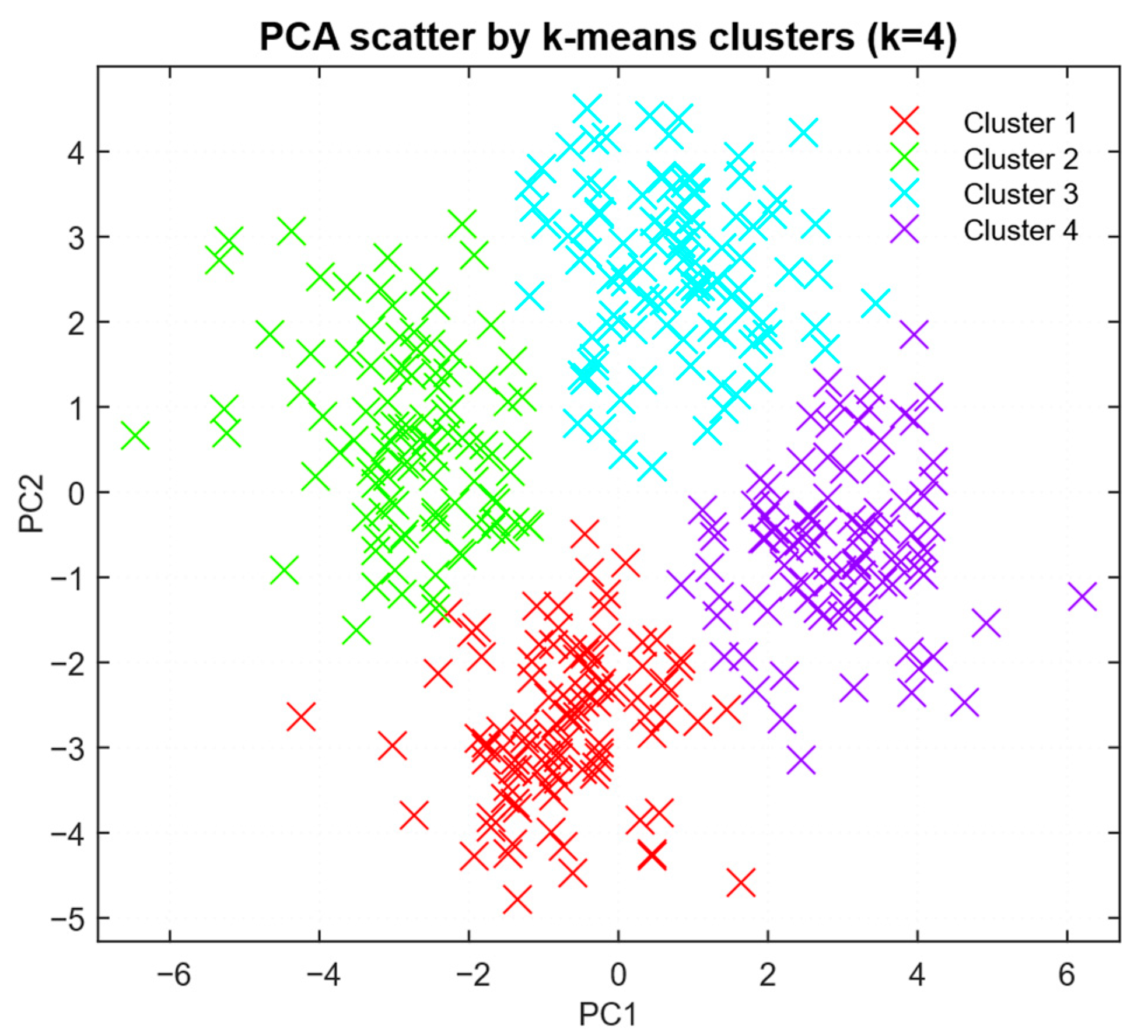
Figure 7 shows the observation distribution across the first two principal components (PC1, PC2), according to the k-means clustering results with k = 4.
According to Figure 7, the observations’ projection onto the first two principal components shows that k-means clustering with k = 4 partially delimits the data. The yellow points are concentrated on the right along the PC1 axis, the purple ones are in the upper central area, while the other two clusters (blue and green) overlap strongly in the centre and left. It indicates that the PC1 direction explains the main structure of the data, but the boundaries between some clusters are not clear. Therefore, the chosen k = 4 captures patterns, but their robustness and suitability should be further verified (silhouette, cluster centre analysis, other projections, or original features).
Figure 8 shows that the average silhouette score increases from k = 2 (≈0.28) to a maximum at k = 5 (≈0.39), after which it decreases monotonically with an increasing number of clusters. The peak at k = 5 indicates the intracluster density and intercluster separation optimal ratio in this range, but the silhouette values themselves (≈0.32–0.39) indicate moderate rather than obvious data structuring.
Thus, the used dataset (see Table 3 and Table 4) is a mixed dataset, of which the central part consists of carefully prepared proprietary telemetry data from EDR platforms (see Figure 5) (≈70,000 sequences), supplemented with excerpts from publicly available reproducibility datasets (≈30,000 sequences) with clear labelling by malware families. The combination used allows us to ensure the realism of the production environment and the reproducibility of experiments simultaneously. The dataset was evaluated by malware categories (ransomware, trojan, backdoor, info-stealer, or fileless or LOLBIN activity type). It demonstrated robustness, since the best results were achieved in classic process-oriented scenarios (“create_process”, “write_file”). In contrast, reduced results are shown on fileless attacks and heavily packed (obfuscated) samples, where the explicit API patterns information density is lost. To simulate obfuscation, controlled transformations were introduced in the experiment, namely, code packing (encryption) (destructive loss of static indicators), argument randomisation, insertion of noise calls, and modification of time intervals (Δt jitter). The proposed approach demonstrated advantages in Δt-aware processing and significance selection, as it compensates for some of the noise through temporal aggregation and cumulative statistics.

3.2. Results of the Developed Neural Network Training

To train the developed neural network (see Figure 1), the study used its hyperparameters, which are given in Table 8. It is noted that the hyperparameter selection and tuning methodology in this study is based on careful parameter selection to ensure high model performance when working with API call sequences. Key hyperparameters such as embedding size, the LSTM layer number, regularisation coefficients, and temporal modification parameters (e.g., a time-aware kernel) were used to improve the model’s ability to capture both short-term and long-term dependencies.
As a training rate scheduler strategy, it is recommended to use a linear warm-up during the first ~5% steps up to the specified maximum training rate, and then cosine annealing from lrmax to lrmin (e.g., 10−6). If there is no improvement in the validation metric for a long time, you can additionally enable ReduceLROnPlateau (factor 0.5, patience is 10).
During its training, diagrams of monitoring metrics, precision, recall, F1-score, ROC AUC, per-class F1, average detection time (detection delay), and false alarm rate (FAR) over time were obtained, which are presented in Figure 9.
Figure 9a demonstrates the increase in the metric values (precision, recall, F1-score, AUC ROC, per-class F1-score, average detection delay, false alarm rate, ROC curve, and loss function) during the training epochs, which indicates a consistent improvement in the neural network training accuracy and recall. ROC AUC values exceeding 0.9–0.92 by the training end confirm the developed neural network’s (see Figure 1) high discriminatory ability. Figure 9b demonstrates an increase in classification according to the Benign class relative to the Malware class, which is explained by the data imbalance and greater predictability of standard sequences. At the same time, the gradual increase in the F1-score for Malware indicates that the developed neural network learns to identify rare but informative attack patterns. According to Figure 9c, the decrease in the average detection time from ~10 to ~3 s as optimisation proceeds indicates the developed neural network time-aware architecture’s effectiveness in accelerating the response to threats, which suggests an improvement in the statistical evidence accumulation rate when using modified LSTM cells (see Figure 2) and attention blocks. According to Figure 9e, the ROC curve deviates slightly from the diagonal, and the AUC values ≈ 0.9–0.95 confirm high class separability. It demonstrates the developed neural network’s (see Figure 1) ability to effectively (at least at the 90–95% level) distinguish malicious and benign API call sequences at different thresholds. It is also noted that the loss function dynamics obtained (Figure 9e) on the training dataset monotonically decreases to the 0.18–0.24% level, and on the validation dataset it stabilises at a slightly higher level (at the level of 0.23–0.28%), which indicates a developed neural network (see Figure 1) with high generalising ability. The curves’ substantial divergence absence (the divergence does not exceed 1.17–1.28 times) indicates that the developed neural network (see Figure 1) is not prone to overfitting with the selected hyperparameters (see Table 8).
A comparative analysis of the quality metrics of the developed neural network (see Figure 1) with other neural network architectures used to solve similar problems was performed on the training dataset (see Table 3). A traditional recurrent neural network without modifications [38] is capable of modelling the dependence between successive API calls but loses efficiency (accuracy drops below 81–84%) for long sequences and does not take into account the time intervals between events. LSTM models show moderate accuracy (approximately at the level of 85–87%) and increased detection time due to weak sensitivity to rare informative patterns.
Convolutional neural networks [11] applied to tokenised API sequences are good at detecting local n-gram patterns of calls (accuracy exceeds 92%), which is critical when analysing short fragments (the length of such pieces does not exceed 20 tokens). However, CNNs poorly capture long-term dependence and temporal structure (accuracy does not exceed 70%), which leads to a higher level of false alarms (up to 10%) and, as a result, limited generalisation ability.
The self-attention-based architecture (without recurrent connections) [16] provides high accuracy (in the 90–95% range) and explainability due to global attention. However, the analysis of system call tasks requires extensive data and computing resources, and without an additional time-aware module, it processes real intervals between events poorly (accuracy falls below 90%).
The developed neural network (see Figure 1) is based on the multi-branch recurrent time-modified blocks and salience gate combination, which allows modelling both short and long dependencies by integrating information about Δt delays. Adding time-aware attention ensures interpretability and speeds up detection, reducing latency and the number of false positives.
It is noted that the model demonstrated high detection performance on the original data but is vulnerable to domain shift, strong imbalance, and adversarial transformations, as its performance declines primarily in recall on rare families and during long sessions. The implementation of targeted measures, such as fine-tuning on small domain labels, self-supervised pretraining, reweighting, focal loss, and sequence-aware augmentations for rare classes, as well as local or linear attention optimisation, consistently restored generalisation performance without significantly increasing the false alarm rate. Adversarial training and test-time adaptation improve robustness to evasion patterns, while ensembles and calibration methods (MC dropout, temperature scaling) provide a reliable uncertainty estimate. Therefore, it is advisable to apply data-level correction and fine-tuning in stages, then domain alignment and adversarial methods, with continuous monitoring of per-class recall and time-to-detection to ensure stability in real and hostile conditions.
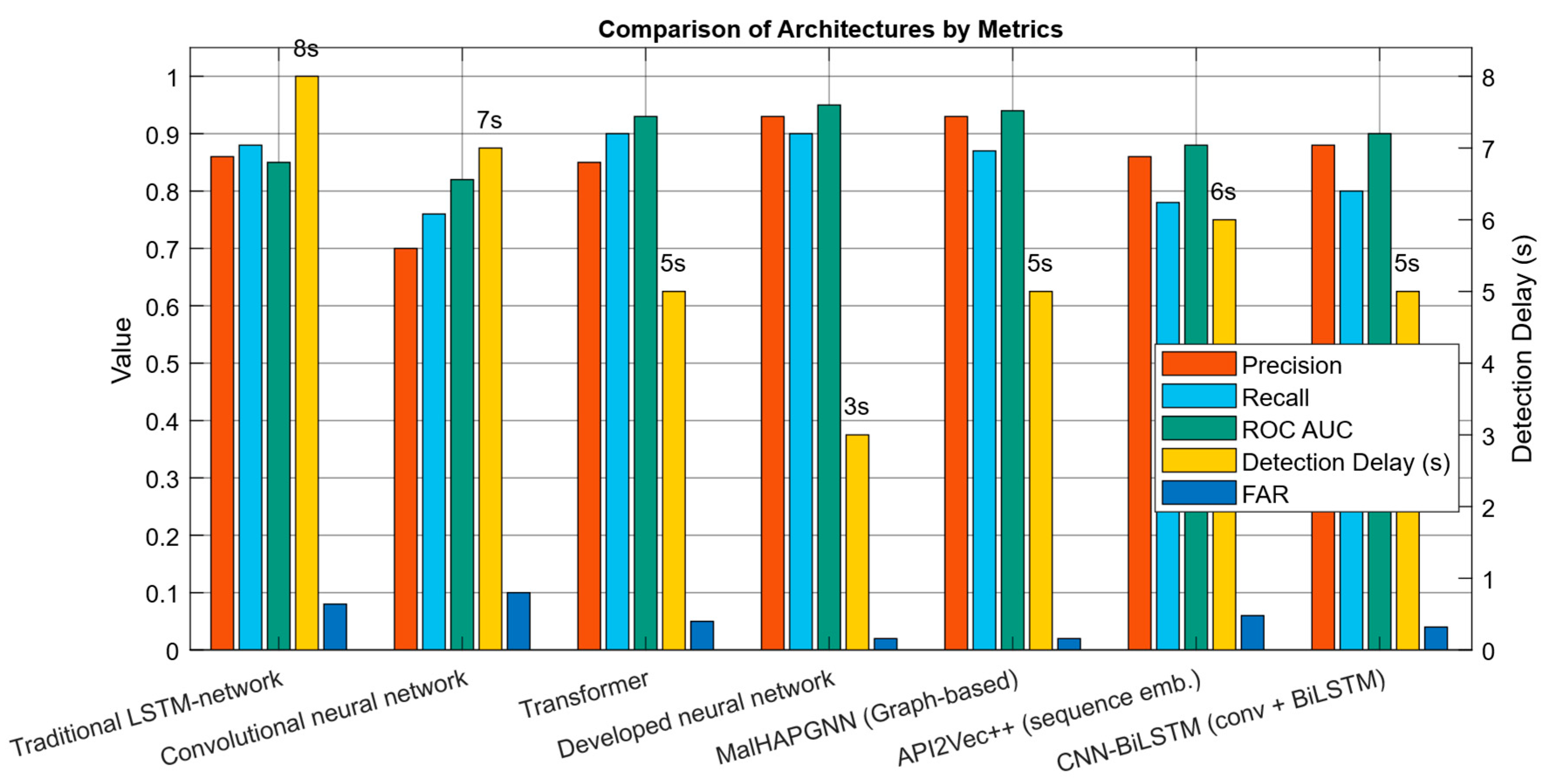
Table 9 presents the comparative analysis results, and Figure 10 shows a graph comparing the key metrics (precision, recall, AUC, Delay, and FAR) values for the four neural network architectures considered.
The comparative analysis revealed significant differences in the neural network architectures’ performance when detecting malicious API call sequences. The traditional LSTM network [38] demonstrated moderate results, since the precision was 0.80, the recall was 0.72, and the AUC was 0.85. At the same time, the average detection time remained high (>8 s), and the false alarm rate was about 8%. The convolutional neural network [11] application showed average precision (0.78) and recall (0.70) but demonstrated the worst FAR (10%) and average detection latency of about 7 s, which is due to the limited ability of convolutions to model long-term dependencies. Transformer (self-attention-based architecture) [16] provided a noticeable improvement, because the precision reached 0.90, the recall was 0.85, the AUC was 0.93, and the average latency was reduced to 5 s with a false alarm rate of about 5%. MalHAPGNN (graph-based, heterogeneous API call GNN) takes into account structural relationships between API calls, models context as a heterogeneous graph, and demonstrates high performance in semantically rich scenarios (precision is 0.91, recall is 0.87, AUC is 0.94, latency is 5 s, low FAR is 3%) but requires expensive graph preprocessing and more memory. API2Vec++ (sequence embedding with a classifier) forms compact vector representations of sequences and provides fast inference; however, it may lose some information about the order and intervals in the original logs (approximate precision is 0.86, recall is 0.78, AUC is 0.88, latency is 6 s, and FAR is 6%). The CNN-BiLSTM hybrid combines the advantages of convolutions (catches local patterns) and bidirectional LSTM (context in both directions), showing balanced results (approximately precision is 0.88, recall is 0.84, AUC is 0.90; latency is 5 s, FAR is 4%) in a more complex setting. However, high computational complexity and the lack of explicit accounting for time intervals remained limiting factors. The developed neural network showed the best results, since the accuracy was 0.93, recall was 0.88, and AUC was 0.95, while the average detection time was only 3 s, and the FAR decreased to 2%. Thus, the developed neural network (see Figure 1) not only ensures higher classification accuracy (at the level of 93% and above) but also significantly reduces the delay in threat detection (up to 3 s), which makes its use appropriate for practical online analytics systems.

3.3. Results of an Example Solution to the Detecting Malware Problem by the API Requests Analysis Sequences

An example of detecting malware problem-solving based on the API call sequences analysis is shown. The study uses a given dataset (see Table 4). It demonstrates the stages of preprocessing, embedding construction, and the attention and salience mechanism for interpretability, as well as an online detector based on CUSUM and accompanying visualisations (length histograms, top APIs, PCA, attention heatmap, CUSUM, salience, and confusion matrix).
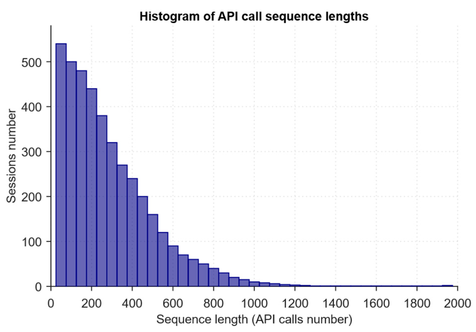
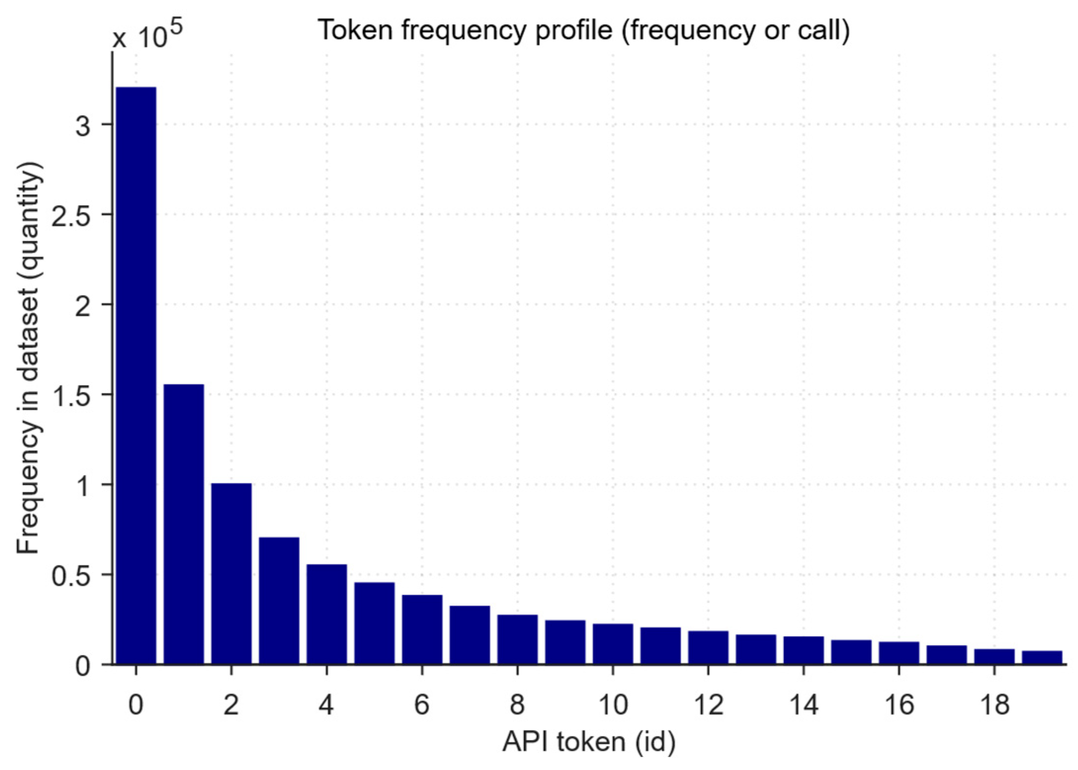
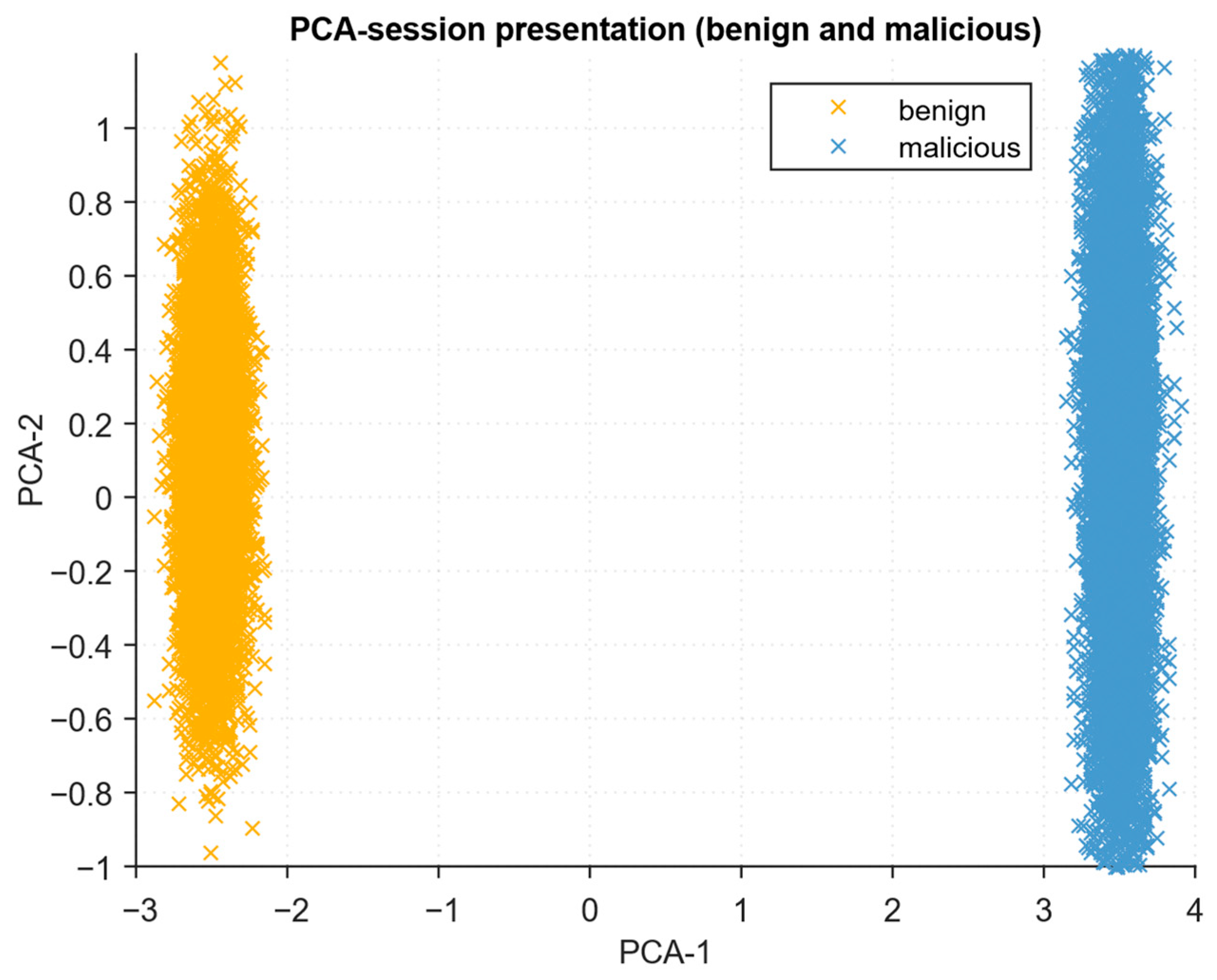
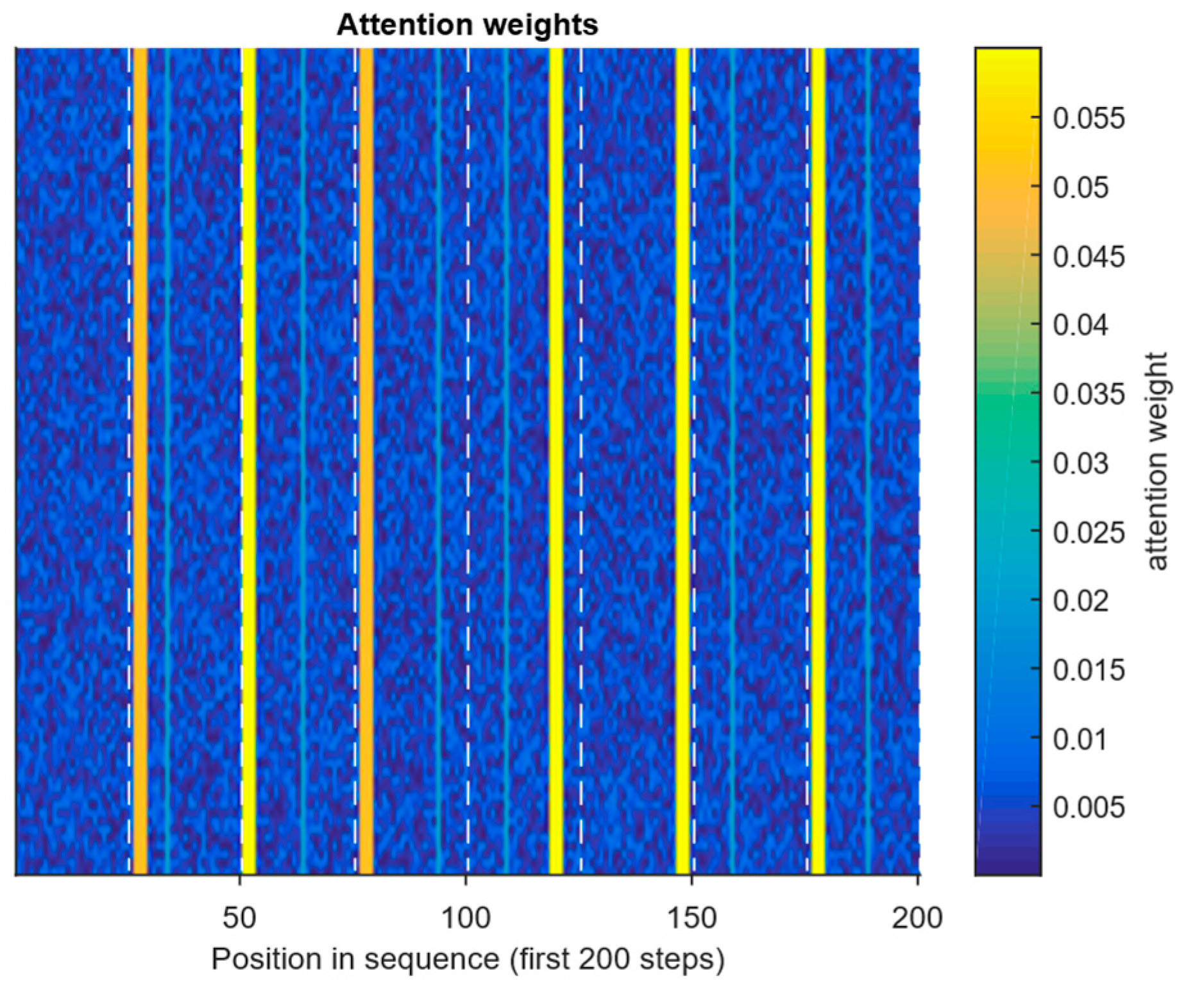
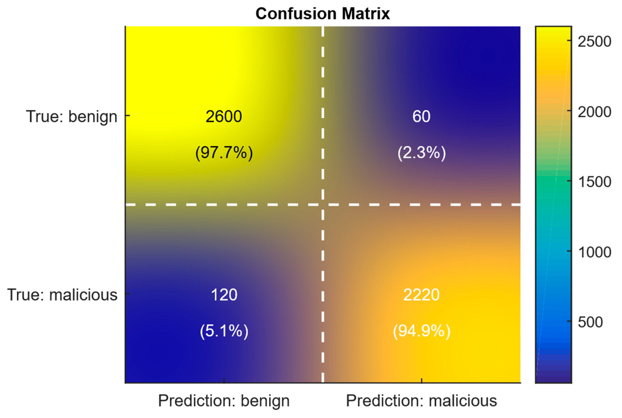
The resulting graphs illustrate the API sequence length distribution (heavy-tailed) (Figure 11), token frequency profile (top 20 dominant API calls) (Figure 12), 2D visualisation of embeddings (benign and malicious separability) (Figure 13), attention heatmap (Figure 14), and salience gate time series for localising informative steps (Figure 15), as well as the CUSUM criterion with marked trigger points (Figure 16) and confusion matrix (Figure 17). The results show that embeddings allow the identification of suspicious clusters, and spikes in attention (salience) often precede the detector threshold exceedance.
The sequence length histogram (Figure 11) shows a pronounced heavy-tailed distribution, since most sessions are concentrated in the ≈100–600 calls range, with rare, very long sessions up to ~2000 calls. It dictates the need for adaptive preprocessing (bucketing), dynamic padding or windowing, and taking into account memory limitations (latency) for the online mode. A practical consequence is that the model should be validated separately on short, medium, and long sessions, since its behaviour may differ significantly.
The tokens’ frequency profile confirms strong frequency non-uniformity (Figure 12), as a few tokens dominate and many tokens are rare. It complicates the embeddings training, as frequent tokens are approximated better and rare ones worse, so subsampling of frequent tokens, frequency smoothing, or pretraining of embeddings are useful. In analytics, it is essential to distinguish between the dominant APIs’ contribution (the noise signals source) and rare “flag” APIs, which are often more informative for detection.
The PCA projection of embeddings (Figure 13) shows a discernible clustering of malicious sessions forming a separate region, which indicates potential separability of classes in the embedding space and the simple classifiers’ effectiveness on these features. However, visual separation may reflect side factors (session length, context), so it is necessary to control for confounders and estimate separability metrics (e.g., silhouette, inter-centroid distances) on stratified subsamples. It provides a practical basis for using linear and nonlinear classifiers as a baseline.
The attention heatmap (Figure 14) shows rare, sharp peaks of attention, i.e., the model concentrates on individual tokens (positions) rather than distributing weights evenly—consistent with the idea that attacks manifest themselves through rare “signal” events. The resulting peaks are helpful in interpreting and localising suspicious moves. Still, attention alone does not guarantee causality, so it is necessary to verify the peaks’ correlation with known compromise indicators. Technically, it makes sense to control for the peaks’ tendency to frequent tokens (entropy regularisation or multi-head attention).
Salience gate (Figure 15) provides a smoothed activity signal, whose peaks coincide with the zones of increased attention and often precede the CUSUM growth, i.e., the modules work in concert and localise the “zones of interest.” Such a signal is convenient for segmenting sessions and implementing early-exit logic or operational verification of selected fragments. It is essential to choose a threshold for salience based on benign or malicious distributions to minimise the number of false peaks.
The CUSUM diagram (Figure 16) illustrates the statistics accumulation and a sharp threshold exceedance at the information burst moments—a successful sequential detector’s typical behaviour. In practice, the threshold h should be calibrated during validation, since raising the threshold reduces false alarms but increases the detection delay, and lowering the threshold has the opposite effect. It is recommended that the delay distribution and inter-alarm intervals be analysed, and a CUSUM reset (inertia) strategy should be introduced after triggering.
The confusion matrix (TN = 2600, FP = 60, FN = 120, TP = 2220) (Figure 17) showed the evaluation metric’s high values, with a precision of ≈97.4%, recall ≈ 94.9%, F1-score ≈ 96.1% and FPR ≈ 2.3%. The obtained results indicate high accuracy (97.4% and higher) and recall (94.9% and higher) in the conducted computational experiment; however, even a small percentage of FN can be critical in practical applications in cyber police.
An analysis of Figure 11, Figure 12, Figure 13, Figure 14, Figure 15, Figure 16 and Figure 17 shows that attention peaks consistently identify individual signalling steps and often precede the CUSUM triggering. Therefore, to assess the significance of an API call at a peak position, the corresponding token should be sequentially extracted, and its frequency position in the corpus should be analysed. Its contribution to the probability of the “malicious” class should be estimated through the odds ratio. With the confidence intervals and significance criteria calculation, the delays distribution between the peak and the CUSUM triggering (median and quantiles) should be studied to understand the operational value of the event, and the frequent “noisy” tokens influence should be taken into account through rank normalisation or the exclusion of stop tokens; in practice, these elements are combined into a scoring function (e.g., “score = w1 · odds_ratio + w2 · salience—w3 · freq_rank”), whose threshold is calibrated during validation. An interactive interface with context export allows for faster manual verification and forensic examination.
The obtained results show that heavy-tailed lengths and Zipf-like token distribution characterise API sequences. At the same time, averaged embeddings allow us to identify separable benign or malicious clusters, and attention peaks and smoothed salience activations localise informative steps that often precede the CUSUM statistics transition through the threshold. In the computational experiment, the method demonstrates high indicators (precision ≈ 97.4%, recall ≈ 94.9%), but even a small share of FN remains a critical factor. In practice, this dictates a two-level strategy for cyber police: an automatic early selection of fragments of interest (embeddings with salience or attention) and subsequent verification by a sequential criterion (CUSUM or SPRT) for generating alerts, with threshold mandatory calibration on deferred data, maintaining an indicators repository (IOCs), logging all intermediate artefacts for forensics, and human support in the loop for confirming critical signals and the model’s continuous retraining.
To verify the explanation’s validity, an objective test set was developed and applied:
  • Perturbation tests include masking and sequentially removing the top-k elements, random elements, and critical API calls; measuring the change in model confidence (a combination of sufficiency (comprehensiveness) and AOPC metrics).
  • Alignment tests involve comparing the attention (or saliency) ranking with the “critical” APIs labelling (precisionk, recallk).
  • Statistical correlation refers to correlating explanation ranks with the expert indicator score (IOC score).
The results showed a stable and quantitatively significant relationship: for attention-based search of the top five tokens, the average sufficiency was ≈ 0.71 (the model retains 71% of the initial confidence when retaining only the top five), comprehensiveness ≈ 0.38 (removing the top five reduces confidence by 38%), and AOPC ≈ 0.30. Precision5 relative to expert-reported critical APIs was ≈0.78, recall5 ≈ 0.64, and the Spearman rank correlation between attention scores and IOC score was ≈0.62 (p < 0.001). The integrated gradient and gradient-based saliency methods demonstrated slightly better sufficiency (comprehensiveness) (≈0.76 and 0.44) and high stability under time jitter and sequence-warp augmentations. However, some deviations were revealed: attention tends to overestimate time markers and frequent service tokens, while saliency better localises rare, semantically significant API calls.
A cross-validation analysis was performed, and the results (five-fold, stratified by families) are as follows: average accuracy is 96.1% ± 0.3%, average ROC-AUC is 0.802 ± 0.012, average PR-AUC is 0.862 ± 0.015, average FAR is 2.7% ± 0.2%, and average detection time (P95 latency) is 4.1 ± 0.3 s). These results confirm the method’s stability when changing samples and demonstrate the reproducibility of the characteristics in different folds. Table 10 shows the cross-validation and ablation analysis results, demonstrating the proposed methods’ stability on various datasets and the quantitative contribution of the architectures’ key components (salience selection, attention mechanism, and CUSUM statistical accumulator) to the final indicators of precision, recall, and false positive rate.
Thus, removing the significance gate results in a significant increase in FAR (+1.1%) and a decrease in PR-AUC (–0.024), indicating the filtering importance of rare, informative events. Removing attention reduces sensitivity to complex intercall dependencies, reducing PR-AUC (–0.021). Removing CUSUM reduces detection latency (–0.9 s) but sharply increases FAR (+2.3%), confirming the cumulative statistics value for robustness.
A comparative analysis of the developed method’s effectiveness in solving the malware problem by API requests analysing sequences with the closest analogues was carried out (Table 11).
Table 11 shows that the Gated Recurrent Unit with Generative Adversarial Network [48] on datasets of ≈ 5000–50,000 samples demonstrates the claimed accuracy of 98.9% (approximately precision ≈ 0.985, recall ≈ 0.989), which indicates very high sensitivity in offline training due to GAN augmentation. Early Malware Detection [49], tested on datasets of ≈21,000–24,000 samples, shows superiority over SOTA, since the precision ≈0.95 and recall ≈ 0.92 values reflect the tradeoff between early detection and recall. Temporal Convolutional Network with Attention [50] shows an accuracy range of ≈90–98% (estimated precision ≈0.92, recall ≈0.90), which emphasises the results’ sensitivity to the corpus and hyperparameter settings. The developed method on the N = 5000 dataset shows an accuracy of ≈96.4%, precision 0.9737, and recall 0.9487, which is 1.5–1.8 times higher than the closest analogues.
A comparison using advanced metrics shows that the model, which demonstrated high ROC-AUC (0.80) and PR-AUC (0.866) with low calibration error (ECE≈0.04) in Table 10, maintains a stable tradeoff between missed and false positives in real-world tests. With a working threshold focused on maximising recall, the false negative rate (FNR) is significantly reduced at the expense of increasing FPR, whereas tuning to minimise false alarms achieves the opposite tradeoff. These dependencies are sensitive to the threshold, class distribution, and session length. Measurements in various deployment scenarios show that FNR and FPR vary linearly with the operating point and data shift, and detection latency depends on the mode. In GPU inference, performance in representative sessions remains within near real-time limits (lower in magnitude than batch processing), whereas with CPU or distributed inference, latency and throughput degrade significantly. Therefore, reporting on specific operating points (threshold, throughput, peak-mem) and splits (short and long sessions, rare classes) is essential. It is promising to expand the comparative analysis by incorporating classical baseline methods and modern architectures (alternative attention schemes, lightweight transformers, and ensembles) to contextualise the improvements and demonstrate robustness across different operating points.
It is noted that it is advisable to conduct experiments in future research in this subject area, since this will allow for a more complete assessment of the model’s resistance to standard obfuscation methods and adversarial attacks, which is an essential aspect for its practical application.

3.4. Results of the Developed Method of Detecting Malware by API Requests, Analysing Sequences, and Computational Complexity Evaluation

To estimate the developed method’s computational complexity, it is assumed that N is the input sequence length (the number of API calls in a session), while the average length is N ¯ = 41,212, and sliding window for online is ≈256; B is the batch size (batch_size = 64); V is the vocabulary size (vocab = 587); E is the token embedding size (embedding_dim = 128); Darg = 64 is the additional arguments projection size; Din = E + Darg is the input size in LSTM (in this research, Din = 128 + 64 = 192); the multi-branch RNN (consisting of LSTM cells) has three branches with hidden state sizes H1 = 128, H2 = 256, and H3 = 128; and attention has the following parameters: “heads” number h = 4, key size dk = 64, and aggregated representation H i = 512 .
The collection of embeddings and projecting of arguments’ computational complexity is estimated as a copy or linear transformation as
T e m b N = O N · E N · E .
The LSTM cell computational complexity at one step (four gates) is estimated as
T L S T M _ s t e p D i n , H 4 · H · D i n + H ,
and for the entire sequence of length N as
T L S T M N , D i n , H N · 4 · H · D i n + H .
Then, for several branches, summation is performed over the branches:
T L S T M _ t o t a l N = i = 1 3 N · 4 · H i · D i n + H i .
Thus, multi-head time-aware self-attention allows explicit encoding time intervals and multi-scale temporal dependencies in each head. It improves the model’s ability to weight temporally relevant events and improves the predictions’ interpretability while maintaining high parallelism. Computationally, the principal components contribute in the order of projections of Q, K, and V, which is O(3 ⋅ Ndmodeldk); dominant matrix multiplications QK and subsequent multiplications with V are VO(hN2dk); and output projection is O N · d m o d e l 2 .
Thus, the MAC operations number provides approximate estimates for the forward pass: an average session length N ¯ = 412, the three LSTM branches’ total cost is approximately 3.24 ⋅ 108 MACs, multi-head time-aware attention is about 2.35 × 10⁸ MACs, and embeddings (projections) and dense layers together are about 5.45 × 10⁷ MACs. As a result, the total forward pass per observation is estimated at approximately 6.14 × 10⁸ MACs. For batch B = 64, this gives ≈ 3.93 × 10¹⁰ MACs, and one epoch on the dataset of ~5000 samples (forward) ≈ 3.07 × 10¹² MACs (taking into account the backward pass, which increases the cost by approximately (2–3)×, the order of costs per epoch will be (6.1–9.2) × 1012 MACs); for online mode with sliding window N = 256, forward ≈ 3.61 × 10⁸ MACs (equivalent to batch B = 64 ≈ 2.31 × 10¹⁰ MACs). The obtained results are calculated for forward pass on the selected hyperparameters, and they highlight the LSTM cells and quadratic attention in N contributions dominance and serve as a basis for choosing optimisations (N constraint, sparse or local attention, mixed precision, checkpointing).
To estimate the memory computational complexity (spatial complexity, main cost drivers), the following model parameters were used: embedding matrix V × E = 587 × 128 ≈ 75,136 parameters; total number of parameters (LSTM, attention, dense) ≈ 2.04 × 10⁶ parameters (≈2.0 M); final volume ≈ 2.0 × 10⁶ float ≈ 8.2 MB (32-bit floats). It is noted that the parameters are estimated based on the developed neural network architecture (see Figure 1).
Activations (peak memory in a batch) that store hidden attention states (and LSTM cells) across all steps requires the following order:
A B · N · d m o d e l   f l o a t s .
For N = 412, dmodel = 512, and B = 64, the value obtained is ≈13.5M float ≈ 51.5 MB for activations only. At the same time, taking into account gradients and the optimiser (when using the Adam optimiser state ×2), the real RAM for training easily reaches several hundred megabytes (≈150–300 MB) and more, depending on the checkpointing depth and other buffers. For online N = 256, it is approximately 32 MB of activations (before taking into account optimiser states).
It is noted that the architecture’s asymptotically main “bottleneck” is the attention mechanism O(hN2dk) quadratic contribution in the sequence length, while the multi-branch LSTM gives a linear contribution in N, formally, O N · i H i · D i n + H i , which rapidly increases by the parameters’ square as the hidden states Hi increase in size. At the same time, the memory for activation scales is O(BNdmodel) and becomes critical when training on large batches and long sessions. As a result, with increasing average session length N, computational and memory-oriented costs grow fastest due to attention and stored activations, which makes it necessary to use engineering solutions consisting of length limiting (sliding window), bucketing with dynamic padding, sparse, local, or linear attention, or hybrid architectures (local attention with recurrent aggregation, Temporal Convolutional Network, or factorised RNN) to bring the cost to linear in N, as well as training optimisation (mixed precision, gradient checkpointing, and reducing batch_size). At the same time, the difference between training and inference (backwards pass, optimiser states) suggests separate optimisation for production mode, namely, implementation profiling, the FP16 or inference accelerators use, and reducing the window in online detection (e.g., Nwin = 256) allows for a significant reduction in the latency without substantial quality loss.
Thus, the developed method demonstrates high discrimination and acceptable online detection latency. Still, its computational cost is dominated by the attention term, quadratic in the sequence length O(hN2dk), which makes training and scaling resource-intensive. Therefore, for practical deployment, it is recommended to preserve the architectural advantages (time-aware attention for interpretability) while limiting the session length (sliding window), using sparse, local, or linear attention or hybrid schemes and engineering optimisations (mixed precision, gradient checkpointing, batch_size reduction, and implementation profiling) to bring the costs to an acceptable level without significant efficiency loss.
In addition to 70–74, real-world hardware profiling was conducted: on an A100 GPU (40 GB), the average training time for one iteration with a 512-layer batch and a model depth of 24 was 142 ms, with memory usage reaching 34.7 GB. On a similar configuration, the TPUv4 achieved 119 ms and 31.2 GB, respectively. The resulting metrics allowed us to identify bottlenecks, including I/O latency of approximately 12% of the total time on the A100 and interconnect bandwidth saturation of 85% on the TPUv4.
For the developed neural network architecture, the key bottleneck in computational and memory terms is the attention complexity O(h · N2 · dk), which is quadratic in the session length. At the same time, LSTM branches provide only linear complexity in N. It is quantified as the multi-headed time-aware attention itself ≈ 2.35 × 10⁸ MACs per session and the total forward pass ≈6.14 × 10⁸ MACs with an average length N ≈ 412 (with a batch of 64, this gives ≈3.93 × 10¹⁰ MACs per iteration), and peak activations in the batch ≈13.5M float (≈54 MB ≈51.5 MiB), with a total training memory size of hundreds of megabytes. Based on this, it is reasonable to replace dense self-attention with economical variants like Longformer (sliding window with global tokens), Linformer (low-rank K, V projection), Performer (kernel-approx), or Reformer (LSH), since they ensure linearity and locality of computation and allow for significant reduction in MACs and peak memory with an acceptable loss of global context. For example, Longformer with a window w = 64 for N = 412 reduces attention operations by approximately 6–7× (2.35 × 108 · (64/412) ≈ 3.65 × 10⁷ MACs instead of 2.35 × 10⁸), which leads to a decrease in the total forward pass to ≈ 4.15 × 10⁸ MACs (≈1.5× speedup) provided that a small number of global tokens are used to restore far context. On large datasets, the current architecture demonstrates good detection power, but suffers from severe computational and memory-oriented limitations, including multi-head attention and being quadratic in session length, dominates the cost of ≈2.35 × 10⁸ MACs per session and ≈6.14 × 10⁸ MACs per forward pass for N ≈ 412 (which, for batch=64, yields ≈3.93 × 10¹⁰ MACs per iteration), and peak activations are on the order of ≈13.5M elements (≈54 MB, ≈51.5 MiB), with a total training memory size of hundreds of megabytes. In practice, this results in low throughput and high GPU requirements (see A100 profiles in the report).

3.5. Results of the Developed Method for Detecting Malware by API Requests, Analysing Sequences Implementation in Forensic Auditing

The developed method is implemented as a specialised software product (Figure 18), which serves as a module for preliminary automated triage analytics in the forensic investigation chain. The developed software product accepts raw dynamic analysis logs (e.g., Cuckoo JSON) or API call traces with saved timestamps, normalises and extracts token sequences and delta times (Δt), passes them through a time-aware LSTM or attention model, and simultaneously tracks online statistics using the CUSUM method. The output is a probabilistic “malicious or benign” assessment, an attention heatmap, and online alarms. All this allows the investigator to quickly see not only the anomaly fact but also which specific calls and time intervals contributed to the solution—important information for a high-quality explanation of the findings in a forensic examination.
In terms of implementation in forensic audit practice, the solution is integrated into the SIEM or SOC pipeline and the electronic evidence lab environment [51,52]. When a new sample or trace dump is received, the system automatically analyses, prioritises, and generates a report with immutable metadata (hashes, source file, model version, timestamps) for the evidence storage chain. The developed software product interface allows analysts to play back a sequence, export attention snapshots and CUSUM diagrams to a report, and manually mark events for subsequent model retraining. Implementation also requires setting false alarm thresholds, documenting model versions, and validation procedures so that model outputs are reproducible and admissible as evidence. Table 12 lists the key components and their role in a forensic audit.
From a practical and legal perspective, implementation requires not only technical integration but also clearly measurable operational metrics and validation procedures. It is reasonable to set TPR requirements above 0.90, FPR in the range <0.05 (adaptable to context), and latency to CUSUM-alarma ≲ 5 s for typical traces as targets for production deployment, as these values are taken as benchmarks for threshold calibration and resource planning [53]. Validation includes end-to-end testing on delayed and real corpora, k-fold validation to assess metric spread, stress tests with adversarial or poisoning scenarios, and stability measurements under different initialisations. Documented verification results and regression test reports should be stored with each model version [54].
In the evidence and reproducibility chain terms, the system should provide immutable logging (WORM or append-only), reports signed with a hardware or cryptographic key (TPM or HSM), and containerised deployment (Docker or Singularity) with described dependencies and a “model card” for each version. For operational work, integration with SIEM or SOC (via Kafka, syslog, or REST), the offline analysis possibility in the lab, and an API for manual audit of events ensure correct examination: the analyst can reproduce the sequence, export heatmap attention and CUSUM graphs, and add annotations that are used for retraining. All these steps are recorded in metadata (hashes, timestamps, and versions), which makes the model’s conclusions reproducible and suitable for forensic justification.
During a prototype’s test deployment, the system demonstrated an average throughput of ≈25,000 system call sequences/second on an A100 GPU with a batch size of 256 and a model depth of 24 layers. Under peak loads, performance dropped to 18,500 sequences/second with an increase in the average online detection latency to 85 ms (versus 42 ms in normal mode). To maintain relevance, the model was retrained every 14 days on an augmented dataset of +12% new traces, including fresh malicious samples and legitimate processes. In between, a continuous learning strategy was employed using experience replay (a buffer of 50,000 examples) and EWC (Elastic Weight Consolidation) regularisation, with a coefficient λ = 100. To eliminate concept drift, we monitored the input features distribution: when a statistical shift in more than 5% in KL divergence was detected, a retraining process was automatically launched, which allowed us to maintain the recall metric above 92% and limit the FNR growth to less than +1.5% during operation for three months.
The hardware set up for the benchmark is described as a single-node configuration with 2×CPU (a total of 64 physical cores, 512 GB DDR4, NUMA), one NVIDIA A100 40 GB (in scalable tests up to 4 × A100 with NVLink), 2 × NVMe PCIe4.0 SSDs (sequential throughput of ≈3.5–7 GB/s), and a 100 GbE network interconnect (RDMA) and InfiniBand HDR for multi-node. Resource metrics are measured using “nvidia-smi”, “psutil”, “perf”, and “iostat”. The dataset contains N = 100,000 API sequences (training is 70,000, validation is 15,000, and testing is 15,000 samples), with an average length of ~120 calls (truncation or padding up to 256). A class imbalance is malicious ≈8%. Preprocessing includes API “tokenisation → embedding”, Δt normalisation, one-hot/ID for arguments, feature engineering, and data augmentation (time jitter, event dropout, windowed shuffling). The measurement methodology is a 120 s warm-up, a 600 s measurement window, and five runs. Load generation is performed via Kafka (or ZeroMQ) with an adjustable ingestion rate of 1 → 30,000 seq/second, online (latency-sensitive) scenarios with batch size one and concurrency of 8, 16, and 32 workers, and batch (throughput) scenarios with batch ∈ {64,128,256} in single- or multi-GPU modes (DataParallel or NCCL), GPU streams 2–4, and pipeline parallelism for multi-GPU. Per-sequence latency (P50, P95, P99), throughput (seq/second), peak and average GPU memory (“nvidia-smi”), CPU utilisation, and end-to-end latency including I/O are measured. All models were run on the same testbed, with identical preprocessing and data, the same warm-up and measurement windows, and a fixed software stack (framework, CUDA, cuDNN, drivers). For the lightweight models, knowledge distillation (KD) with a teacher is a complete model; quantisation (INT8, posttraining quant, or QAT), structured pruning (~50% FLOPs reduction), and early-exit architecture (3-exit shallow branching) were applied. Table 13 compares the developed complete model and its lightweight versions (distillation, quantisation, pruning, and early exit) for key metrics, including throughput, latency (P50, P95, and P99), memory consumption, accuracy, and false positive rate. It allows for evaluating the tradeoffs between speed, resource efficiency, and detection quality.
Based on Table 13, it can be concluded that the balance between latency, throughput, and acceptable false alarm rates determines the choice of specific models. High accuracy and minimal FAR are prioritised by using the complete model (the developed method), which is justified in scenarios involving mission-critical objects. While tasks with strict latency and resource constraints are best addressed using lightweight models (distillation, quantisation, pruning, or early exit), which significantly accelerate processing and reduce memory consumption with a moderate loss of quality. Therefore, the integration of the proposed solutions into practical monitoring and forensics systems should be tailored to specific operational conditions and risk profiles.
Validation protocols included cross-validation, splitting data into training and independent test datasets, and repeatable experiments with fixed random seed values and preservation of original logs, ensuring verifiable reproducibility of results. To meet forensic standards, detection explanations were formalised in documented reports with transparent descriptions of analysis steps, model parameter recording, and immutable event logs, enabling traceability of the evidence chain. Additionally, collaboration with legal professionals and digital forensics experts is envisaged through regular consultations during the data storage and transmission protocols development, joint chain-of-custody audits, and reporting compliance verification with procedural norms. Legal review of the interpretations and conclusions wording is also included to ensure their proper inclusion in criminal or civil case materials. This interaction format allows the methodology to be adapted to the evidence admissibility and proactively eliminates requirements and their challenge risks in judicial practice.
A promising direction is the integration of additional modalities, such as network traffic or file system events, which will improve detection accuracy through cross-domain feature correlation. To reduce false alarms, adaptive thresholds can be dynamically adjusted based on current flow statistics and the exploitation context. Evolving malware tactics are handled through continuous training mechanisms and feature repertoire updates, accounting for concept drift and the emergence of new attack strategies.
Figure 19 and Figure 20 show a timeline of API calls with marker sizes reflecting salience (highlighting informative events), and a salience time series with cumulative CUSUM statistics demonstrating the moments of detector triggering.
In Figure 19, the significance gate is represented by the marker size. In this context, larger markers correspond to higher salience values, that is, events that the model considers informative for detecting malicious behaviour. Figure 19 shows that informative events (e.g., the “create_process” series and sharp “network_connect” clusters) are localised in time and often arrive in clusters, which simplifies local incident aggregation during forensics. Furthermore, the time series (Figure 20) shows the instantaneous salience estimate and cumulative statistics (CUSUM), which accumulates small signals and generates more reliable detections when a threshold is exceeded. This combination helps reduce false alarms, as single high-salience events do not immediately trigger an alert; stable accumulation is required, which improves the practical suitability for operational monitoring systems. Table 14 presents a short sample dataset of API events with the highest salience score (event time, API type, salience value, and recommended action) for forensic triage.
Table 14 provides a practical shortlist of the most informative API events with ready-made recommendations for initial triage. It enables analysts to quickly focus on the most likely incidents and save time during investigation. The high-salience set covers various types of actions (process creation, file writing, network connections, and registry reading), demonstrating that the model captures complex behavioural indicators rather than isolated signatures.
Thus, the obtained results’ scientific novelty lies in the fact that the developed approach is fundamentally different in that it combines a multiscale time-aware LSTM with salience gates, time-aware multi-head attention, and a sequential statistical detector (CUSUM) with a formal justification for preserving “long memory”, which makes it possible to explicitly account for Δt intervals, enhance rare “flag” events, and validate the accumulated statistics. It contrasts with typical CNN-LSTM or GNN schemes with hierarchical attention (contrast) pretraining, which either poorly model real-world time intervals or do not integrate sequential statistics and memory regularisers. Experimentally, this provides significant advantages in terms of accuracy and performance. On the corpus under consideration (N = 5000), the developed system shows 96.4% accuracy (precision is 0.9737, recall is 0.9487, F1-score is 96.1%), and the average detection time is 3 s. FAR is 2.3%, while the closest analogues (GRU with GAN, TCN with attention, classical CNN, LSTM, and transformer architectures) demonstrate either lower accuracy, greater latency, or a higher false alarm rate.

4. Discussion

In this research, a mathematically sound method for dynamic detection of malware based on the Windows API calls time sequences analysis is proposed. The behaviour is defined as a sequence of events with timestamps according to (1)–(3), for which the mapping operator Φ(●) is introduced into a fixed time-aware embedding and subsequent detection via likelihood ratio criteria and sequential tests according to (16)–(20). The theoretically sound requirement for preserving long-term memory is formalised in Theorem 1 (the configuring gates possibility that preserves information over ample time intervals is proven), which provides a basis for working with sparse and delayed attack indicators.
A hybrid neural network architecture is implemented, consisting of a trainable embedding layer, a SpatialDropout1D layer, a multi-branch LSTM stack with a temporal kernel and salience gates, time-aware multi-head self-attention, and dense blocks (see Figure 1, Figure 2 and Figure 3). The model integrates temporal kernels Kτt) according to (48)–(58) and mechanisms that penalise memory decay for necessary steps (regulariser (63)), which increases sensitivity to rare “flag” events. Its training algorithm and step-by-step scheme are described in Table 2, and the primary hyperparameters are in Table 8.
Prefixed and validation-tuned hyperparameters responsible for preprocessing, architecture, training, and online detection were used: session filter by length ≥ 100, API dictionary is 587, online sliding window is 256 with a step of 16, token embeddings of 128 and argument projection of 64 (input to RNN is 192), multi-branch LSTM with hidden state sizes {128, 256, 128}, attention is four heads with key size of 64, temporal kernel function Kτt) = exp(−β · Δt) with β = 0.1, and salience gate is 0.5. Training was performed with Adam (lr = 10−3, β1 = 0.9, β2 = 0.999, ϵ = 10−8), batch size is 64, epochs ≤ 50, early stop (patience=5), gradient clipping is 5, L2 = 10−5, regularisation is SpatialDropout1D (0.15), recurrent dropout is 0.1, and dense dropout is 0.3. Scheduler strategy: linear warm-up (~5% steps), cosine annealing (with possible ReduceLROnPlateau), monitoring, precision, recall, F1, AUC, per-class F1, delay, and FAR metrics definition. For the online detector, CUSUM with Nwin = 256, threshold h = 5, and update at each new z was applied. In contrast, the threshold value was calibrated during validation to achieve the target FAR ≈ 0.02 (target operating points and thresholds are fixed during validation and documented along with the throughput and peak-mem profiles).
It has been experimentally shown that the time-aware LSTM and attention combination provides a significant improvement compared to traditional architectures. The developed network achieves a precision of 0.93, a recall of 0.88, and an ROC AUC of 0.95 with an average detection time of ≈3 s, and FAR is 2% (the comparative analysis results are given in Table 9 and the corresponding graphs in Figure 9 and Figure 10). At the same time, the loss function, monotonic stabilisation, and metrics growth were observed during training. The ROC AUC is stably > 0.9, and the average detection delay decreased from ~10 to ~3 s during optimisation, which confirms its practical suitability for online detection.
The developed method (see Figure 3) synthesis includes a data extraction from the Cuckoo pipeline (see Table 3 and Figure 5), preprocessing (filtering seq_length ≥100, the dictionary tokenisation from 587 API), and a combined decision mode: a neural network classifier with accumulated statistics (LRT or CUSUM) for early response according to (18)–(20).
To improve robustness, a three-stage approach is used:
  • Embeddings pretraining on a large corpus (self-supervised) to speed up convergence and rich representations (see Figure 11 and Figure 12);
  • Sequence augmentation (cropping, time-warping, masking, rare pattern oversampling) for robustness to incomplete and distorted logs (see Figure 13, Figure 14 and Figure 15);
  • Adversarial training (FGSM- or PGD-like and sequential counterexamples, ~10–30% of the batch) to reduce vulnerability to targeted traversals (see Figure 16 and Figure 17).
An analytical evaluation shows that the total computational complexity consists of the linear in N LSTM contributions according to (71)–(73) and the dominant quadratic in length attention term O(h · N2 · dk) according to (70), which makes the attention mechanism the primary “bottleneck” in long sessions. Therefore, the research proposes engineering measures for practical deployment: length limitation (sliding window), bucketing with dynamic padding, the sparse, local, or linear attention, and training or inference optimisations (mixed precision, gradient checkpointing, batch_size reduction), which allow for a substantial reduction in the computational and memory-oriented load. The results confirm the significance of these optimisations, since at N ≈ 412 the accumulated activations are estimated to be in the tens of megabytes (≈13.5M float ≈ 51.5 MB for activations, while the total training memory is hundreds of MB). At the same time, the online window mode (Nwin = 256) significantly reduces memory requirements and latency.
From the forensic audit viewpoint, the developed software product is designed for integration into the expertise pipeline. The online triage module generates a probabilistic assessment, heatmap attention, and CUSUM signals for localising informative steps (see Figure 14, Figure 15, Figure 16 and Figure 18), which facilitate explainability and experts’ practical work. Thus, combining the neural network assessment with accumulated sequential statistics (log ratio, SPRT, or CUSUM according to (16)–(20)) enables early response with controlled FAR.
Thus, the research contribution is the development of a theoretically sound and practically implemented method for detecting malware by system call sequences, which combines several innovations:
  • A theoretical result on the preservation of long-term memory possibility in gated recurrent cells (Theorem 1) is introduced and proved, which justifies the architectural choice.
  • A multi-branch time-aware RNN architecture is proposed based on a modified LSTM with salience gates and a time kernel, integrated with time-aware multi-head self-attention for explicitly taking into account the intervals Δt and the critical steps’ interpretability.
  • The sequence embedding operator Φ is formalised, and additional loss regularisers (terms) are introduced, increasing the embeddings’ interclass dispersion and resistance to noise and obfuscation.
  • A hybrid detector is proposed that combines a neural network classifier with sequential criteria (LRT or CUSUM) for online response.
  • A pipeline for data extraction from Cuckoo, preprocessing procedures, and augmentation techniques (adv-training) to improve robustness was implemented.
It would also be advisable to consider integrating data from various sources beyond Cuckoo Sandbox, which would allow us to test the proposed model’s robustness in multiple environments and for various malware types. This expansion will help increase the algorithm’s versatility and demonstrate its ability to adapt to new threats. An important area of focus will also be improving the model’s accuracy in the limited data and changing attack strategies faced, which is also addressed in research on the WAFBooster use, which explores automatically strengthening web application protection against mutating malicious payloads.
Despite this research’s significant contribution to the information security field, the research has a number of limitations, which are presented in Table 15. At the same time, Table 16 presents a roadmap for future research aimed at eliminating the described limitations.
Thus, this research proposes a theoretically sound time-aware RNN architecture with salience gates and a hybrid detector that achieves high accuracy and practical applicability for online malware detection.
It is also noted that the developed method can integrate adaptive learning and certified security methods. To achieve this, the system incorporates a module for monitoring input data distributions (e.g., using the Population Stability Index or Jensen–Shannon divergence). When thresholds are exceeded, this module automatically initiates local retraining of the model using a recent API call sequence buffer. This retraining is performed with a reduced training rate (training rate is 10−5–10−6) and L2-norm regularisation of the base model weights, which reduces the catastrophic forgetting risk. A dynamic ensemble is used: lightweight submodels (distilled or quantised) trained on the most recent N = 10,000–20,000 examples are added to the base model. During inference, the system aggregates its responses, increasing resilience to local data shifts. Robust training is used to protect against targeted attacks. It involves generating adversarial sequences (e.g., inserting false API calls or artificially distorting Δt time intervals) and adding them to the training dataset. Certified robustness guarantees are provided through formal verification methods (e.g., calculating upper bounds on Lipschitz constants for recurrent blocks and attention). It allows for demonstrably limiting the obfuscation impact or input data modification within the ε-neighbourhood. This solution combines practical adaptivity (dynamic updating) with formal robustness guarantees, making the system ready for use in active adversarial environments.

5. Conclusions

The theorem of the long-term memory property of gated recurrent cells is formalised and proved to provide long-term memory in gated recurrent cells with correct gate settings. Regularisers are proposed to preserve significant memory components (salience penalty) and distance metrics (Kulback–Leibler divergence, Wasserstein distances) and are used as an additional objective function to increase interclass separability.
A method based on the multiscale time-aware LSTM with salience gates, multi-headed attention mechanism, and sequential change detector CUSUM integration is developed, which provides a simultaneous solution to three problems: robust modelling of long behavioural sequences, interpretable localisation of informative events, and early statistical detection of anomalies with low latency. This approach allowed us to achieve high accuracy (F1-score ≈ 96%) while maintaining operational requirements for latency (≈3 s) and the level of false alarms (FPR ≈ 2–3%).
The developed time-aware architecture (multi-scale LSTM with salience gates, time-aware multi-head attention, and online CUSUM detector) provides interpretability and early warning due to the following mechanism. At the same time, the attention heatmap highlights rare attention-sharp peaks (≈5% of positions in the session), which localise individual “signal” API steps, and the salience gate forms an activity-smoothed time profile, of which peaks are consistent with increased attention and statistically often precede the CUSUM statistics growth. In the conducted computational experiment, the first CUSUM alarm was recorded around step 180, despite the fact that attention and salience peaks occurred earlier.
The developed time-aware architecture significantly reduces the detection delay, since the average detection time dropped from ~10 to ~3 s during optimisation, while the ROC AUC is in the ≈0.90–0.95 range. Therefore, the developed method is advisable to use for online analytics with low latency requirements.
It is found that the dataset characteristics impose a limitation on the models’ generalisability, since the API sequences have heavy-tailed lengths (“min” is 100, “median” is 310, “max” is 2000), the dictionary is covered by ≈96% (565 out of 587), while there is a strong frequency unevenness (Gini is 0.72), and the average pairwise Jaccard is 0.11. It requires bucketing or dynamic padding, class weighting, and embeddings pretraining for adequate generalisation.
It is established that the developed method is vulnerable to obfuscation and adversarial techniques. It is shown that data augmentation, adversarial training, and contrastive or self-supervised pretraining are required to eliminate this limitation. It is also necessary to take into account the computational complexity and introduce operational requirements (e.g., TPR > 0.90, FPR < 0.05, latency ≲ 5 s), immutable logging, and a “model card” for forensic reproducibility.

Author Contributions

Conceptualisation, S.V., M.N. and V.V. (Victoria Vysotska); methodology, S.V. and V.V. (Victoria Vysotska); software, M.N., V.V. (Vitalii Varlakhov), V.V. (Victoria Vysotska), S.B. and V.P.; validation, V.V. (Vitalii Varlakhov), S.B. and V.P.; formal analysis, S.V.; investigation, S.V., V.V. (Vitalii Varlakhov), V.V. (Victoria Vysotska), S.B. and V.P.; resources, S.V., M.N., S.B. and V.P.; data curation, S.V., M.N. and V.V. (Victoria Vysotska); writing—original draft preparation, S.V.; writing—review and editing, M.N., V.V. (Vitalii Varlakhov), S.B. and V.P.; visualisation, M.N., and V.V. (Victoria Vysotska); supervision, V.V. (Vitalii Varlakhov), S.B. and V.P.; project administration, S.V.; funding acquisition, M.N. All authors have read and agreed to the published version of the manuscript.

Funding

This research received no external funding.

Data Availability Statement

Data is contained within the article.

Acknowledgments

The research was carried out with the grant support of the Ministry of Education and Science of Ukraine, “Methods and tools for detecting disinformation in social networks based on deep learning technologies” under Project No. 0125U001852. During the preparation of this manuscript, the authors used [ChatGPT 4o Available, Grammarly, and Gemini 2.5 flash] to correct the style and improve the quality of the text, as well as to eliminate grammatical errors. The research results obtained in the article are entirely original. The authors have reviewed and edited the output and take full responsibility for the content of this publication.

Conflicts of Interest

The authors declare no conflicts of interest.

Appendix A

Let us have a standard LSTM cell of the following form (considered single level, in which scalar notations can be generalised to vectors):
i t = σ ( W i · x t + U i · h t 1 + b i ) , f t = σ ( W f · x t + U f · h t 1 + b f ) , o t = σ ( W o · x t + U o · h t 1 + b o ) , c ~ t = tanh W c · x t + U c · h t 1 + b c , c t = f t c t 1 + i t c ~ t , h t = o t tanh c t ,
where σ is the sigmoid, ⊙ is the element-wise multiplication.
We define the state ctk contribution to the current state ct as
I t , k c t c t k .
From the recurrence equation, it is easy to obtain the following (scalar version, generalises to vectors or matrices along the diagonal):
I t , k = j = 0 k 1 f t j .
Thus, the previous state decays (or is preserved) contribution as the forget gate’s product over the interval.
The definition (measure of memory retention) is carried out by determining the memory retention coefficient for a fixed k-th lag as
M R k = E I t , k = E j = 0 k 1 f t j ,
where the mathematical expectation is taken over a sample or batch and over components (in the vector case, it is the average over the vector elements or the norm) if MR(k) decreases exponentially with k, which means the network is losing long-term memory.
To evaluate the importance of regularisations’ impact, we assume that scalar importances st ∈ [0, 1] are given (e.g., the importance attentional estimate of an input at time t for a future target feature), and we introduce a regulariser that encourages the preservation of information at those times where st is large. In this context, the regularisations’ specific form is
L r e g = λ · t s t · 1 f t 2 2 ,
In the vector case, ft is a forget-gates vector, and the norm is applied per component. The log f t 2 , or the Kullback–Leibler penalty is also applied. Then the whole optimisation problem is represented as
min θ L t a s k θ + L r e g θ ,
from which solution it follows that the penalty minimises the forget-gate deviations from 1, where st is large, that is, it reduces the product f “attenuation” rate for essential steps.
Assertion. Let ft ∈ (0, 1] be a random variable with finite moments, and let the regulariser L r e g = λ · t s t · 1 f t 2 be introduced, where st ≥ 0 are the given significance weights. Suppose that during optimisation with this regulariser, the conditional second moment E 1 f t 2 s t decreases in absolute value depending on λ (the larger λ, the greater the decrease). Then, for any lag k and for those positions j = 0, …, k−1 where stj are large, the logarithm is introduced. The contributions’ logarithm expected value is
log I t , k = j = 0 k 1 f t j
Which increases compared to the variant without regularisation, and therefore E [It,k] also increases.
Proof. 
It is assumed that δt:= 1 − ft and that δt is small (i.e., ft is close to 1) or, more formally, δt is bounded in absolute value. Then, by Taylor series expansion around 1,
log f k = log 1 δ t = δ t 1 2 · δ t 2 + o δ t 2 .
Calculating the sum of the logarithms, the mathematical expectation, we obtain
E log I t , k = j = 0 k 1 E log I t , k j = 0 k 1 E δ t j + 1 2 · E δ t j 2 + o max j E δ t j 2 .
The regulariser Lreg directly penalises the δ t 2 values with the weight st, so with successful optimisation, we expect a decrease in E δ t 2 in those steps where st is large. However, for most optimisation schemes, this also entails a decrease in E [δt] or does not increase it significantly. Consequently, for intervals where stj are high, the expression E δ + 1 2 · E δ 2 becomes “less negative”, i.e., E log I t , k increases relative to the case without regularisation. Since the exponential function is monotonic, this leads to an increase in E I t , k = E exp log I t , k > E I t , k without regularisation. Therefore, all other things being equal E log I t , k with regularisation> E log I t , k without regularisation. □
The Table A1 shows the mean values and standard deviations of the metrics obtained from three independent runs for each model.
Table A1. The regularisation impact assessment results.
ModelMR(10)MR(50)MR(100) k 1 2 (Timesteps)Delayed-Task ACC (K = 100)MSE (K = 100)
Standard LSTM0.42 ± 0.030.11 ± 0.020.03 ± 0.0123 ± 20.62 ± 0.020.41 ± 0.05
LSTM with regularisation (λ = 0.1, st hard)0.56 ± 0.020.22 ± 0.030.08 ± 0.0237 ± 30.73 ± 0.020.32 ± 0.04
LSTM with regularisation (λ = 0.5, st hard)0.63 ± 0.020.30 ± 0.030.22 ± 0.0254 ± 40.79 ± 0.010.26 ± 0.03
LSTM with regularisation (adaptive st via attention)0.60 ± 0.020.28 ± 0.030.11 ± 0.0349 ± 30.77 ± 0.020.28 ± 0.03
Thus, significant regularisation increases MR(k) at all lags, increases the effective half-life of k 1 2 , and improves accuracy in the long-lag problem. The strengthening of this effect with increasing λ demonstrates that the “memory preservation vs. training flexibility” tradeoff is manageable.

References

  1. Yang, B.; Yu, Z.; Cai, Y. Malicious Software Spread Modeling and Control in Cyber–Physical Systems. Knowl.-Based Syst. 2022, 248, 108913. [Google Scholar] [CrossRef]
  2. Zhang, S.; Wu, J.; Zhang, M.; Yang, W. Dynamic Malware Analysis Based on API Sequence Semantic Fusion. Appl. Sci. 2023, 13, 6526. [Google Scholar] [CrossRef]
  3. Anđelić, N.; Baressi Šegota, S.; Car, Z. Improvement of Malicious Software Detection Accuracy through Genetic Programming Symbolic Classifier with Application of Dataset Oversampling Techniques. Computers 2023, 12, 242. [Google Scholar] [CrossRef]
  4. Amer, E.; Zelinka, I.; El-Sappagh, S. A Multi-Perspective Malware Detection Approach through Behavioral Fusion of API Call Sequence. Comput. Secur. 2021, 110, 102449. [Google Scholar] [CrossRef]
  5. Zhang, D.; Zhang, Z.; Jiang, B.; Tse, T.H. The Impact of Lightweight Disassembler on Malware Detection: An Empirical Study. In Proceedings of the 2018 IEEE 42nd Annual Computer Software and Applications Conference (COMPSAC), Tokyo, Japan, 23–27 July 2018; pp. 620–629. [Google Scholar] [CrossRef]
  6. Amer, E.; Zelinka, I. A Dynamic Windows Malware Detection and Prediction Method Based on Contextual Understanding of API Call Sequence. Comput. Secur. 2020, 92, 101760. [Google Scholar] [CrossRef]
  7. Syeda, D.Z.; Asghar, M.N. Dynamic Malware Classification and API Categorisation of Windows Portable Executable Files Using Machine Learning. Appl. Sci. 2024, 14, 1015. [Google Scholar] [CrossRef]
  8. Zhang, S.; Gao, M.; Wang, L.; Xu, S.; Shao, W.; Kuang, R. A Malware-Detection Method Using Deep Learning to Fully Extract API Sequence Features. Electronics 2025, 14, 167. [Google Scholar] [CrossRef]
  9. Zhang, R.; Huang, S.; Qi, Z.; Guan, H. Combining Static and Dynamic Analysis to Discover Software Vulnerabilities. In Proceedings of the 2011 Fifth International Conference on Innovative Mobile and Internet Services in Ubiquitous Computing, Seoul, Republic of Korea, 30 June–2 July 2011; pp. 175–181. [Google Scholar] [CrossRef]
  10. Shijo, P.V.; Salim, A. Integrated Static and Dynamic Analysis for Malware Detection. Procedia Comput. Sci. 2015, 46, 804–811. [Google Scholar] [CrossRef]
  11. Ali, M.; Shiaeles, S.; Bendiab, G.; Ghita, B. MALGRA: Machine Learning and N-Gram Malware Feature Extraction and Detection System. Electronics 2020, 9, 1777. [Google Scholar] [CrossRef]
  12. Guo, W.; Du, W.; Yang, X.; Xue, J.; Wang, Y.; Han, W.; Hu, J. MalHAPGNN: An Enhanced Call Graph-Based Malware Detection Framework Using Hierarchical Attention Pooling Graph Neural Network. Sensors 2025, 25, 374. [Google Scholar] [CrossRef]
  13. Aggarwal, S.; Di Troia, F. Malware Classification Using Dynamically Extracted API Call Embeddings. Appl. Sci. 2024, 14, 5731. [Google Scholar] [CrossRef]
  14. Anil Kumar, D.; Das, S.K.; Sahoo, M.K. Malware Detection System Using API-Decision Tree. Lect. Notes Data Eng. Commun. Technol. 2022, 86, 511–517. [Google Scholar] [CrossRef]
  15. Cui, L.; Yin, J.; Cui, J.; Ji, Y.; Liu, P.; Hao, Z.; Yun, X. API2Vec++: Boosting API Sequence Representation for Malware Detection and Classification. IEEE Trans. Softw. Eng. 2024, 50, 2142–2162. [Google Scholar] [CrossRef]
  16. Yang, J.; Jiang, X.; Liang, G.; Li, S.; Ma, Z. Malicious Traffic Identification with Self-Supervised Contrastive Learning. Sensors 2023, 23, 7215. [Google Scholar] [CrossRef]
  17. Yang, S.; Yang, Y.; Zhao, D.; Xu, L.; Li, X.; Yu, F.; Hu, J. Dynamic Malware Detection Based on Supervised Contrastive Learning. Comput. Electr. Eng. 2025, 123, 110108. [Google Scholar] [CrossRef]
  18. Berrios, S.; Leiva, D.; Olivares, B.; Allende-Cid, H.; Hermosilla, P. Systematic Review: Malware Detection and Classification in Cybersecurity. Appl. Sci. 2025, 15, 7747. [Google Scholar] [CrossRef]
  19. Shaukat, K.; Luo, S.; Varadharajan, V. A Novel Method for Improving the Robustness of Deep Learning-Based Malware Detectors against Adversarial Attacks. Eng. Appl. Artif. Intell. 2022, 116, 105461. [Google Scholar] [CrossRef]
  20. Nikolova, E. Markov Models for Malware and Intrusion Detection: A Survey. Serdica J. Comput. 2023, 15, 129–147. [Google Scholar] [CrossRef]
  21. Abanmi, N.; Kurdi, H.; Alzamel, M. Dynamic IoT Malware Detection in Android Systems Using Profile Hidden Markov Models. Appl. Sci. 2022, 13, 557. [Google Scholar] [CrossRef]
  22. Maniriho, P.; Mahmood, A.N.; Chowdhury, M.J.M. API-MalDetect: Automated Malware Detection Framework for Windows Based on API Calls and Deep Learning Techniques. J. Netw. Comput. Appl. 2023, 218, 103704. [Google Scholar] [CrossRef]
  23. ALGorain, F.T.; Clark, J.A. Bayesian Hyper-Parameter Optimisation for Malware Detection. Electronics 2022, 11, 1640. [Google Scholar] [CrossRef]
  24. Vladov, S.; Shmelov, Y.; Yakovliev, R. Method for Forecasting of Helicopters Aircraft Engines Technical State in Flight Modes Using Neural Networks. CEUR Workshop Proc. 2022, 3171, 974–985. Available online: https://ceur-ws.org/Vol-3171/paper70.pdf (accessed on 6 August 2025).
  25. Zhang, Y.; Yang, S.; Xu, L.; Li, X.; Zhao, D. A Malware Detection Framework Based on Semantic Information of Behavioral Features. Appl. Sci. 2023, 13, 12528. [Google Scholar] [CrossRef]
  26. Coscia, A.; Lorusso, R.; Maci, A.; Urbano, G. APIARY: An API-Based Automatic Rule Generator for Yara to Enhance Malware Detection. Comput. Secur. 2025, 153, 104397. [Google Scholar] [CrossRef]
  27. Li, N.; Lu, Z.; Ma, Y.; Chen, Y.; Dong, J. A Malicious Program Behavior Detection Model Based on API Call Sequences. Electronics 2024, 13, 1092. [Google Scholar] [CrossRef]
  28. Li, C.; Lv, Q.; Li, N.; Wang, Y.; Sun, D.; Qiao, Y. A Novel Deep Framework for Dynamic Malware Detection Based on API Sequence Intrinsic Features. Comput. Secur. 2022, 116, 102686. [Google Scholar] [CrossRef]
  29. Miao, C.; Kou, L.; Zhang, J.; Dong, G. A Lightweight Malware Detection Model Based on Knowledge Distillation. Mathematics 2024, 12, 4009. [Google Scholar] [CrossRef]
  30. Vladov, S.; Sachenko, A.; Sokurenko, V.; Muzychuk, O.; Vysotska, V. Helicopters Turboshaft Engines Neural Network Modeling under Sensor Failure. J. Sens. Actuator Netw. 2024, 13, 66. [Google Scholar] [CrossRef]
  31. Han, W.; Xue, J.; Wang, Y.; Liu, Z.; Kong, Z. MalInsight: A Systematic Profiling Based Malware Detection Framework. J. Netw. Comput. Appl. 2019, 125, 236–250. [Google Scholar] [CrossRef]
  32. Vaddadi, S.A.; Arnepalli, P.R.R.; Thatikonda, R.; Padthe, A. Effective Malware Detection Approach Based on Deep Learning in Cyber-Physical Systems. Int. J. Comput. Sci. Inf. Technol. 2022, 14, 1–12. [Google Scholar] [CrossRef]
  33. Vladov, S.; Shmelov, Y.; Yakovliev, R. Modified Helicopters Turboshaft Engines Neural Network On-board Automatic Control System Using the Adaptive Control Method. CEUR Workshop Proc. 2022, 3309, 205–224. Available online: https://ceur-ws.org/Vol-3309/paper15.pdf (accessed on 12 August 2025).
  34. Rashid, M.U.; Qureshi, S.; Abid, A.; Alqahtany, S.S.; Alqazzaz, A.; ul Hassan, M.; Al Reshan, M.S.; Shaikh, A. Hybrid Android Malware Detection and Classification Using Deep Neural Networks. Int. J. Comput. Intell. Syst. 2025, 18, 52. [Google Scholar] [CrossRef]
  35. Han, W.; Xue, J.; Wang, Y.; Huang, L.; Kong, Z.; Mao, L. MalDAE: Detecting and Explaining Malware Based on Correlation and Fusion of Static and Dynamic Characteristics. Comput. Secur. 2019, 83, 208–233. [Google Scholar] [CrossRef]
  36. Ilić, S.; Gnjatović, M.; Tot, I.; Jovanović, B.; Maček, N.; Gavrilović Božović, M. Going beyond API Calls in Dynamic Malware Analysis: A Novel Dataset. Electronics 2024, 13, 3553. [Google Scholar] [CrossRef]
  37. Daeef, A.Y.; Al-Naji, A.; Chahl, J. Lightweight and Robust Malware Detection Using Dictionaries of API Calls. Telecom 2023, 4, 746–757. [Google Scholar] [CrossRef]
  38. Akhtar, M.S.; Feng, T. Detection of Malware by Deep Learning as CNN-LSTM Machine Learning Techniques in Real Time. Symmetry 2022, 14, 2308. [Google Scholar] [CrossRef]
  39. Vladov, S.; Vysotska, V.; Sokurenko, V.; Muzychuk, O.; Nazarkevych, M.; Lytvyn, V. Neural Network System for Predicting Anomalous Data in Applied Sensor Systems. Appl. Syst. Innov. 2024, 7, 88. [Google Scholar] [CrossRef]
  40. Kim, H.; Kim, M. Malware Detection and Classification System Based on CNN-BiLSTM. Electronics 2024, 13, 2539. [Google Scholar] [CrossRef]
  41. Li, W.; Tang, H.; Zhu, H.; Zhang, W.; Liu, C. TS-Mal: Malware Detection Model Using Temporal and Structural Features Learning. Comput. Secur. 2024, 140, 103752. [Google Scholar] [CrossRef]
  42. Qian, L.; Cong, L. Channel Features and API Frequency-Based Transformer Model for Malware Identification. Sensors 2024, 24, 580. [Google Scholar] [CrossRef]
  43. Lu, J.; Ren, X.; Zhang, J.; Wang, T. CPL-Net: A Malware Detection Network Based on Parallel CNN and LSTM Feature Fusion. Electronics 2023, 12, 4025. [Google Scholar] [CrossRef]
  44. Vladov, S.; Shmelov, Y.; Petchenko, M. A Neuro-Fuzzy Expert System for the Control and Diagnostics of Helicopters Aircraft Engines Technical State. CEUR Workshop Proc. 2021, 3013, 40–52. Available online: https://ceur-ws.org/Vol-3013/20210040.pdf (accessed on 18 August 2025).
  45. Ferdous, J.; Islam, R.; Mahboubi, A.; Islam, M.Z. A Survey on ML Techniques for Multi-Platform Malware Detection: Securing PC, Mobile Devices, IoT, and Cloud Environments. Sensors 2025, 25, 1153. [Google Scholar] [CrossRef]
  46. Lytvyn, V.; Dudyk, D.; Peleshchak, I.; Peleshchak, R.; Pukach, P. Influence of the Number of Neighbours on the Clustering Metric by Oscillatory Chaotic Neural Network with Dipole Synaptic Connections. CEUR Workshop Proc. 2024, 3664, 24–34. Available online: https://ceur-ws.org/Vol-3664/paper3.pdf (accessed on 19 August 2025).
  47. Vladov, S.; Shmelov, Y.; Yakovliev, R. Optimization of Helicopters Aircraft Engine Working Process Using Neural Networks Technologies. CEUR Workshop Proc. 2022, 3171, 1639–1656. Available online: https://ceur-ws.org/Vol-3171/paper117.pdf (accessed on 21 August 2025).
  48. Owoh, N.; Adejoh, J.; Hosseinzadeh, S.; Ashawa, M.; Osamor, J.; Qureshi, A. Malware Detection Based on API Call Sequence Analysis: A Gated Recurrent Unit–Generative Adversarial Network Model Approach. Future Internet 2024, 16, 369. [Google Scholar] [CrossRef]
  49. Alshomrani, M.; Albeshri, A.; Alturki, B.; Alallah, F.S.; Alsulami, A.A. Survey of Transformer-Based Malicious Software Detection Systems. Electronics 2024, 13, 4677. [Google Scholar] [CrossRef]
  50. Wang, Z.; Guan, Z.; Liu, X.; Li, C.; Sun, X.; Li, J. SDN Anomalous Traffic Detection Based on Temporal Convolutional Network. Appl. Sci. 2025, 15, 4317. [Google Scholar] [CrossRef]
  51. Ablamskyi, S.; Tchobo, D.L.R.; Romaniuk, V.; Šimić, G.; Ilchyshyn, N. Assessing the Responsibilities of the International Criminal Court in the Investigation of War Crimes in Ukraine. Novum Jus 2023, 17, 353–374. [Google Scholar] [CrossRef]
  52. Ablamskyi, S.; Nenia, O.; Drozd, V.; Havryliuk, L. Substantial Violation of Human Rights and Freedoms as a Prerequisite for Inadmissibility of Evidence. Justicia 2021, 26, 47–56. [Google Scholar] [CrossRef]
  53. Lopes, J.F.; Barbon Junior, S.; de Melo, L.F. Online Meta-Recommendation of CUSUM Hyperparameters for Enhanced Drift Detection. Sensors 2025, 25, 2787. [Google Scholar] [CrossRef] [PubMed]
  54. Vladov, S.; Shmelov, Y.; Yakovliev, R.; Petchenko, M.; Drozdova, S. Neural Network Method for Helicopters Turboshaft Engines Working Process Parameters Identification at Flight Modes. In Proceedings of the 2022 IEEE 4th International Conference on Modern Electrical and Energy System (MEES), Kremenchuk, Ukraine, 20–23 October 2022; pp. 604–609. [Google Scholar] [CrossRef]
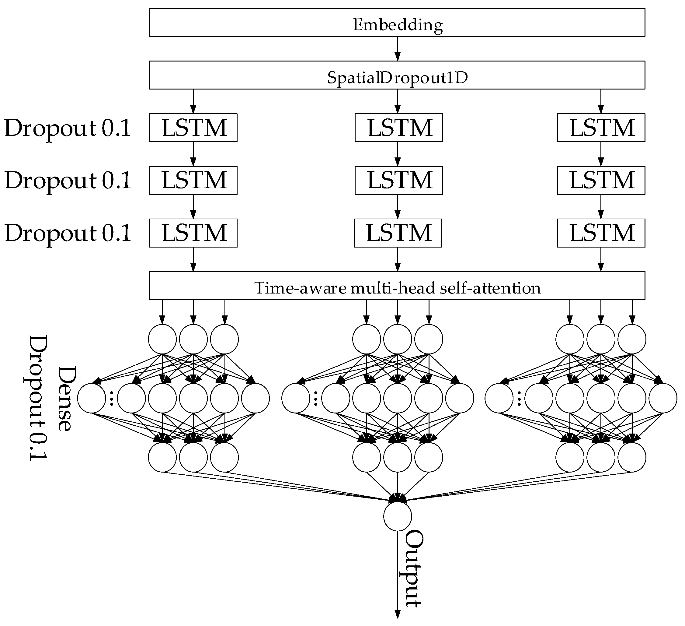
Figure 1. The constructed recurrent neural network architectural diagram.
Asi 08 00156 g001
Figure 2. The developed modified LSTM cell structure.
Asi 08 00156 g002
Figure 3. Structural diagram of the developed method for detecting malware by analysing API requests and analysing sequences.
Asi 08 00156 g003
Figure 4. An experimental sample of the developed method was implemented in the MATLAB Simulink R2014b software environment.
Asi 08 00156 g004
Figure 5. The training dataset preparation using the Cuckoo Sandbox tool follows a general scheme.
Asi 08 00156 g005
Figure 6. The resulting inertia curve.
Asi 08 00156 g006
Figure 7. Diagram of the distribution of observations by the first two principal components.
Asi 08 00156 g007
Figure 8. The resulting average silhouette score.
Asi 08 00156 g008
Figure 9. The main monitoring metrics diagrams: (a) neural network training metrics (precision, recall, F1-score, AUC ROC); (b) per class F1-score; (c) average detection delay; (d) false alarm rate; (e) ROC curve; (f) loss function dynamics.
Asi 08 00156 g009aAsi 08 00156 g009b
Figure 10. Comparison graph for four architectures (traditional LSTM network [38], convolutional neural network [11], transformer (self-attention-based architecture) [16], MalHAPGNN (graph-based, heterogeneous API call GNN), API2Vec++ (sequence embedding with classifier), CNN-BiLSTM (convolutions with bidirectional LSTM), and developed neural network) by five metrics: precision, recall, ROC AUC, detection delay, and FAR.
Asi 08 00156 g010
Figure 11. Histogram of API call sequence length (number of calls).
Asi 08 00156 g011
Figure 12. Token frequency profile (top 20 dominant API calls).
Asi 08 00156 g012
Figure 13. PCA projection of embeddings.
Asi 08 00156 g013
Figure 14. Attention heatmap.
Asi 08 00156 g014
Figure 15. Salience gate diagram.
Asi 08 00156 g015
Figure 16. CUSUM diagram.
Asi 08 00156 g016
Figure 17. Confusion matrix.
Asi 08 00156 g017
Figure 18. The developed software product window.
Asi 08 00156 g018
Figure 19. API event timeline diagram with salience gate highlighting.
Asi 08 00156 g019
Figure 20. Signal significance and cumulative statistics diagram based on CUSUM (detection).
Asi 08 00156 g020
Table 1. Existing research review.
Method (Approach)Data (Features)Model (Architecture)Results ObtainedLimitationsReferences
A combination of static disassembly and dynamicsFeatures from disassembled executables (IDA Pro), API call sequencesClassic classifier with API calls and sequence analysisPractical feasibility, high results on selected datasetsDependent on disassembly quality, static features are subject to obfuscation, and scalability and reproducibility are not always demonstrated[5]
Signature-based approach based on Windows API callsWindows API call sequences and signaturesSignature matching (classifier on signatures)Accuracy ~75–80% by familiesVulnerable to signature changes, obfuscation, and polymorphism, weak overall generalisation[6]
Detection of anomalies in system behaviourOperational system events: registry, file (network) anomalies, telemetryAnomaly algorithms (behaviour classifiers)Can catch polymorphic (metamorphic) samplesNoise in telemetry, false positives; requires careful threshold tuning[7]
Visualisation of behaviour (CNN networks)Extracted API calls and signatures, encoding into imagesConvolutional neural network>90% on selected datasetsDependent on the coding scheme, sensitive to preprocessing, and possible retraining on specific datasets[8]
A hybrid approach of static and dynamic analysisStatic features and execution dynamicsCombined models (ensemble)Improves detection completeness in some casesIntegration complexity, computational costs, and features heterogeneity[9,10]
Sequence representations (n-grams, diagrams, embeddings)API n-grams, call graphs, API vector embeddingsCNN networks, graph neural networks, embeddings and classifiersIncreases the expressiveness of featuresLoss of global context (n-grams), diagram construction complexity, and need for embeddings pretraining[11,12,13]
Classical ML (trees, boosting) on featuresManual feature set, behaviour aggregatesDecision Trees, Random Forest, Gradient BoostingStable results with limited dataRequire careful feature engineering, limitations for long sequences[14,15]
Self-supervised and contrastive pretrainingUnlabelled API log files, events, sequence segmentsPretraining (masked, contrastive) and fine-tuningReduced need for labelled data, better embeddingsNeed for a large amount of unlabelled data; fine-tuning of pretraining tasks[16,17]
Resistance to adversarial attacks and obfuscationModified and attack samplesAdversarial training, robustification techniquesPartial increase in robustnessDecreased overall accuracy, adversarial generation, and robustness assessment are of high complexity[18,19]
Table 2. Developed an algorithm for neural network training.
Layer (Stage)Training Stage DescriptionWhat Is Being Optimised
Input (Preprocessing)API calls tokenisation (indexes, padding, masking, batch formation).Preparing masks and batches (bucketing) for efficient computation.
EmbeddingThe indices are converted into dense vectors. In the forward pass, it produces embeddings, and in the backwards pass, the gradients update the embedding matrix.We can use pre-trained embeddings or train jointly, and we can regularise with dropouts.
SpatialDropout1D (Regularisation)During training, it turns off random embedding channels to reduce feature correlation.Reduces overfitting, affects forward pass only (stochasticity).
Stacked LSTM (Parallel Branches)Sequences pass through multiple LSTM layers; each cell computes hidden states (forward) and receives gradients (backprop) to update the recurrent connection weights.Different branches can have various depths or context lengths (short-term or long-term). Use recurrent dropout and gradient clipping.
Per-branch Dense with DropoutDense layers transform high-level representations from the LSTM. Dropout extinguishes some neurons during training.Provides a nonlinear combination of features and additional regularisation.
Fusion (Attention)Merging branches (concatenation and averaging) and using an attention mechanism to weight the contributions of individual segments and branches. During training, attention weights are also optimised.Attention increases interpretability and focuses on informative fragments.
Output Layer (Classification)In the forward pass, predictions are made, and in the backwards pass, gradients are calculated for the entire network.The activation function and output structure are selected for the task (binary or multi-class).
Loss and Optimiser (Outside Layers)Based on the predictions, a loss (weighted cross-entropy, etc.) is calculated. The Adam optimiser updates all parameters based on the gradients.Setting up LR (LR-scheduler, early stopping, checkpoints).
Additional: Augmentation (Adversarial)During the training process, modified sequences (insertions, permutations, adversarials) can be added to increase robustness.Increases resistance but requires quality control of augmentations.
Table 3. Input dataset.
Data NameData TypeDescriptionValueNotes
sample_idline_intUnique record (file) identifierfile_000123Corresponds to one Cuckoo JSON report.
labelcategoricalMarkup: benign or maliciousmaliciousThe final label for training (or validation).
api_sequencearray_intIndexed API calls (tokens) sequence[12, 5, 233, 17, ...]Tokenisation was performed using the call dictionary. Records with < 100 calls were filtered.
seq_lengthintSequence length (number of API calls)312For selection: seq_length ≥ 100.
timestampsarray_floatTimestamps (the moment each call was executed)[0.003, 0.052, 0.210, ...]Used for time-aware models or Δt calculations.
api_argsstructured JSON (dict)Additional call attributes (arguments, PID, packet sizes, etc.){“pid”:1024, “arg0”:“C:\\temp\\a.exe”}Can be partially normalised (projected) into vector rk.
cuckoo_metadatadictCuckoo metadata: vm_id, run_id, timestamp, scenario{“vm”:“vm01”,”run”:“r123”,”ts”:“2024-01-10T12:00Z”}Stored in PostgreSQL JSON report.
raw_report_pathstring (path)Path to the original JSON report in the database (file system)/cuckoo/reports/r123.jsonFor re-analysis (audit).
extraction_timedatetimeExtraction time (record induction)2024-02-01T09:00ZLog for reproducibility.
notesstringAdditional notes (e.g., filtering, incomplete data)filtered: <100 callsConvenient for debugging the pipeline.
Table 4. Training dataset compiled for sample_id = file_000003.
PositionToken_Index (Value)Timestamp (Seconds)
1120.0018
250.0042
32330.0105
4170.0150
54000.0203
6580.0237
74120.0312
82330.0450
9770.0521
102100.0600
11180.0610
123050.1205
13760.1210
144890.2300
151020.2355
16120.2400
173330.6000
18870.6055
194010.6100
2050.9000
Table 5. The training dataset homogeneity assessment results.
MetricDefinitionValue at N = 5000Interpretation
Class balanceShare of benign or maliciousbenign 58% (2900),
malicious 42% (2100)
Moderate imbalance. Class weights or rare class oversampling during training must be taken into account.
Sequence length (seq_length): min, median, mean, max, stdAPI calls spread in a sessionmin = 100,
median = 310,
mean = 412,
max = 2000,
std = 260
Significant length variability. Bucketing or dynamic padding control is required. However, a high CV (≈ 0.63) indicates non-uniformity of time profiles.
Average unique tokens per sampleHow many samples cover the dictionary locallymean = 178,
std = 95
Large variance. Some samples contain a few different APIs, while others contain many, making it difficult to generalise the model.
Vocab coverageUnique APIs found share in the dataset 565 587 ≈ 96%Almost the entire vocabulary is used, which is positive for training embeddings.
Average entropy of token distribution (per-sample)Token frequency diversity measure in a dataset (bits)mean H ≈ 5.1 byte,
std ≈ 0.9
Moderately high diversity of calls within sessions. Low entropy in some samples indicates a few APIs’ dominance.
Gini coefficient of token frequencies (over the entire dataset)Token frequency distribution unevennessGini ≈ 0.72Strong unevenness: a small number of “frequent” APIs dominate, and the majority are rare.
Average pairwise Jaccard similarity token-set/pairAverage intersection (union) of unique APIs between pairs of samplesmean J ≈ 0.11Low similarity between samples indicates high content variability and weak homogeneity.
Short (noisy) reports (after filtering) presenceShare of calls dropped by the rule < 100~8–12% of original reportsFiltering removed some of the “noisy” short sessions, but the rest are still uneven.
Table 6. K-means clustering results.
kInertia (SSE)Avg. Silhouette
21.42 × 1040.312
39.85 × 1030.367
47.40 × 1030.394
56.10 × 1030.381
65.30 × 1030.362
Table 7. Results of the clusters and the centroid sizes are determined for k = 4.
ClusterSizeSeq_Length (Centre)Unique_Tokens (Centre)Entropy (Centre)Top_Token_Frac (Centre)
0810220854.20.34
111504201705.20.24
29807602606.00.18
356013504107.10.12
Table 8. Primary hyperparameters of the developed neural network.
StageParameterValue
Preprocessingminimum session length100
API dictionary587
sliding window for online256
sliding step16
Embeddings and architecturetoken embedding size128
argument projection64
entry into a recurrent block128 + 64 = 192
Multi-branch RNN (consisting of LSTM cells)hidden_short128
hidden_mid256
hidden_long128
Attentionheads number4
key size64
Time-kernel и salienceexponential decayKτt) = exp(−β · Δt) with β = 0.1
salience gate coefficient0.5
Training and optimisationoptimiserAdam
initial LR10−3
batch_size64
epochs≤50
early-stop patience5
gradient clipping5
L2 weight decay10−5
β10.9
β20.999
ϵ10−8
Regularisation and balancingSpatialDropout1D0.15
recurrent dropout0.1
dense dropout0.3
Online detectorwindow size for online aggregation (Nwin)256
CUSUM threshold h5 (calibrated during validation to achieve target FAR)
detector update rateon every new z
target FAR (benchmark)≈0.02
Table 9. Results of neural network architectures comparative analysis.
ArchitectureStrengthsLimitationsMetrics Values
Traditional LSTM network [38]Simplicity, robustness, and local dependencies captureData loss of information over long sequences, time insensitivityPrecision ≈ 0.80,
Recall ≈ 0.72,
AUC ≈ 0.85,
Detection delay > 8 s, FAR ≈ 0.08
Convolutional neural network [11]Good at detecting local patterns (n-grams), high speedNo long-term memory, weak Δt accountingPrecision ≈ 0.78,
Recall ≈ 0.70,
AUC ≈ 0.82,
Detection delay ≈ 7 s, FAR ≈ 0.10
Transformer (self-attention-based architecture) [16]High accuracy, global dependencies, and explainabilityHigh resources, poor Δt accounting without modificationsPrecision ≈ 0.90,
Recall ≈ 0.85,
AUC ≈ 0.93,
Detection delay ≈ 5 s, FAR ≈ 0.05
MalHAPGNN (Graph-based, Heterogeneous API call GNN)Takes into account the structural relationships of API calls and the graph contextGraph construction and preprocessing are more expensive and are also sensitive to noise and incomplete logs, requiring memory for large sessionsPrecision ≈ 0.91,
Recall ≈ 0.87,
AUC ≈ 0.93,
Detection delay ≈ 5 s, FAR ≈ 0.03
API2Vec++ (sequence embedding with classifier)Compact vector representations of sequences, fast inference, and classificationMay lose order and spacing (unless time-aware is extended); worse with very long (or noisy) sessionsPrecision ≈ 0.86,
Recall ≈ 0.78,
AUC ≈ 0.88,
Detection delay ≈ 6 s, FAR ≈ 0.06
CNN-BiLSTM (convolutions with bidirectional LSTM)Combines local patterns (CNN) and context (BiLSTM).More difficult to set up, higher latency than pure CNNs, sensitive to noisePrecision ≈ 0.88,
Recall ≈ 0.84,
AUC ≈ 0.90,
Detection delay ≈ 4–6 s, FAR ≈ 0.04
Developed a neural networkBalance of short and long dependencies, Δt accounting, interpretability, and low latencyMore complex implementation, need to configure additional hyperparametersPrecision ≈ 0.93,
Recall ≈ 0.88,
AUC ≈ 0.95,
Detection delay ≈ 3 s, FAR ≈ 0.02
Table 10. Ablation results (components’ contributions).
ArchitectureAccuracy (%)ROC-AUCPR-AUCFAR (%)P95 Latency (Seconds)
Complete model (salience, attention, and CUSUM)96.40.8030.8662.54.2
Without salience gate (attention and CUSUM)94.90.7810.8423.64.0
Without attention (salience and CUSUM)95.10.7840.8453.34.1
without CUSUM (salience and attention)95.50.7890.8514.83.3
Table 11. Comparative analysis results of the developed method with the closest analogues.
MethodDataset (Amount)Detection ModeAccuracyPrecisionRecallKey Numerical Indicators
Gated Recurrent Unit with Generative Adversarial Network [48]≈5000–50,000 samplesbatch (offline)98.9%0.9850.989The GAN augmentation with GRU encoder use allowed for achieving significant improvement in quality (accuracy and recall exceed 90%).
Early Malware Detection [49]≈21,000–24,000 samplesearly (few-shot)95.4%0.950.92The fine-tuned transformer (GPT-2) with Bi-RNN and attention application is focused on early API prediction.
Temporal Convolutional Network with Attention [50]≈3000–40,000 samplesbatch (near-online)92.2%0.920.90Parallelism and low latency, while the attention introduction allows for interpretability.
Developed methodN = 5000,
vocab = 587
online or early (attention, salience, CUSUM)96.4%0.97370.9487Mean seq len = 411.32, Median = 346; Max = 2000, PCA centroid dist = 5.598, PCA silhouette = 0.948, attention peak ≈ 5%, CUSUM first alarm ≈ 180; confusion matrix TN = 2600, FP = 60, FN = 120, TP = 2220.
Table 12. Components’ list and their forensic functions.
ComponentFunction in Forensic Audit (Benefits for the Expert)
Parser and NormaliserOriginal timestamps preservation, formats unification
Feature ExtractionReproducible input data preparation
Time-Aware Model with an Attention MechanismClassification, explanations (which events are essential)
Online CUSUMEarly detection of anomalies in real time
VisualisationTriage, replay, evidence export
Export (Evidence Database)Immutable reports storage, model versions, trust chain
Table 13. Results of the comparative indicators evaluation of the developed complete model and lightweight versions (distillation, quantisation, pruning, early-exit) for key metrics.
Model VariantThroughput (Batch is 256) Seq/SecondOnline Latency P50, P95, and P99 (Seconds)Peak GPU Mem (GB)Avg GPU Mem (GB)Accuracy (%)FAR (%)
Complete model (multi-scale time-aware LSTM with attention and CUSUM)25,0002.8, 4.2, and 6.5222096.42.5
Knowledge Distillation (KD, 4× smaller)80,0000.9, 1.6, and 2.88694.83.5
Quantised INT8 (post-train or QAT)60,0001.1, 1.9, and 3.26595.63.0
Pruned (structured, ~50% FLOPs)45,0001.2, 2.0, and 3.510995.92.9
Early-exit architecture (adaptive inference)130,0000.6, 1.1, and 2.0121195.03.2
Table 14. A short sample dataset of API events with the highest salience score.
Time, SecondsAPI EventSalienceSuggested Triage Action
27.432create_process0.97Immediately check child processes and the command line
29.011write_file0.94Extract file, check hashes and contents
33.201load_library0.91Check loaded DLLs for known indicators
40.512network_connect0.89Network metadata collection (IP, port), domain analysis
66.980read_registry0.86Check modified registry keys and modification times
82.114open_file0.83Compare with the allowlist, check access
104.256query_handles0.79Evaluate which descriptors are being requested, search for anomalies
Table 15. Main limitations of the research.
NumberLimitationBrief Explanation (Impact)
1Limited generalisabilityThe model was trained primarily on Windows behavioural traces (Cuckoo), which creates a decreased accuracy risk and an increase in the number of false classifications when transferred to other operating systems, alternative sandboxes, or real endpoint data without additional adaptation.
2Vulnerability to strong obfuscation and adversarial attacksWhen deliberately modifying system call sequences (polymorphism, aggressive obfuscation, targeted adversarial distortions), the probability of a false negative (FN) increases significantly, which leads to a decrease in completeness (recall) while maintaining the apparent reliability of the trace.
3High computational requirements and online detection latenciesUsing time-aware RNNs in combination with multi-head attention and sequential statistical criteria increases the load on the GPU and CPU. It may lead to latencies incompatible with high-throughput environments.
4Dependence on data quality and relevanceThe class imbalance presence, noise in the labelling, and the concept drift phenomenon (software evolution and the emergence of new types of attacks) reduce the models’ stability and require regular dataset updates and additional training to maintain high accuracy.
Table 16. Roadmap for future research.
NumberLimitationAimTasksMetrics
1Limited generalisability (portability to other operating systems or endpoints)Increase the models’ portability across different platforms and real endpoint data(1) Collection of cross-platform datasets (Windows, Linux, Android) and real endpoint data;
(2) Development of domain-adaptation or domain-generalisation (adversarial, MMD, meta-learning) for embeddings;
(3) Validation on hold-out platforms and field sets
Increase in AUC (recall) on new platforms ≥ 10% vs. baseline;
Reduced degradation during transfer (drop ≤ 5%)
2Vulnerability to strong obfuscation and adversarial attacksEnsure resistance to obfuscation and targeted sequence distortions(1) Creation of attacks or obfuscations set (call proxying, noise injection, time-warp);
(2) Adversarial training with adversarial augmentation (seq2seq or perturbation);
(3) Certified research (verifiable) defences (robustness certificates for sequences);
(4) Attack detectors integration
False-Negative reduction under attack ≥ 30% compared to the unattended model;
Certified change margin (if applicable)
3High computational requirements and online detection latencyReduce latency and resource consumption without a significant quality loss(1) Model bottleneck profiling;
(2) Model compression research: knowledge distillation, quantisation, pruning, early-exit;
(3) Online pipeline implementation and optimisation (streaming inference, batching policies);
(4) Testing on target devices (edge, SIEM)
50% latency reduction and/or 2x memory and CPU reduction with ≤ 3% accuracy loss
4Dependence on the quality and relevance of data (concept drift)Ensure that the model adapts to drift and changing threats(1) Development of a drift monitoring system (statistical tests, embedding drift);
(2) Continuous or incremental learning methods (continual learning, replay buffers, regularisers against catastrophic forgetting);
(3) Collection automation and “new” examples annotation;
(4) Regular validation and triggers for retraining
Drift response time (from detection to update) ≤ specified SLA;
Maintaining metrics (AUC or recall) within specified limits when new classes appear
5Cross-cutting activities (infrastructure, replication, open benchmarks)Speed up research and results verification(1) Creation of a reproducible software system or external storage devices for experiments;
(2) External validation organisation
A repository with a dataset (scripts) and external replication availability; adoption of the benchmark in the community
Disclaimer/Publisher’s Note: The statements, opinions and data contained in all publications are solely those of the individual author(s) and contributor(s) and not of MDPI and/or the editor(s). MDPI and/or the editor(s) disclaim responsibility for any injury to people or property resulting from any ideas, methods, instructions or products referred to in the content.