Hybrid Model-Based Traffic Network Control Using Population Games

Abstract

Modern traffic management requires sophisticated approaches to address the complexities of urban road networks, which continue to grow in complexity due to increasing urbanization and vehicle usage. Traditional methods often fall short in mitigating congestion and optimizing traffic flow, inducing the exploration of innovative traffic control strategies based on advanced theoretical frameworks. In this sense, we explore different game theory-based control strategies in an eight-intersection traffic network modeled by means of hybrid systems and graph theory, using a software simulator that combines the multi-modal traffic simulation software VISSIM and MATLAB to integrate traffic network parameters and population game criteria. Across five distinct network scenarios with varying saturation conditions, we explore a fixed-time scheme of signaling by means of fictitious play dynamics and adaptive schemes, using dynamics such as Smith, replicator, Logit and Brown–Von Neumann–Nash (BNN). Results show better performance for Smith and replicator dynamics in terms of traffic parameters both for fixed and variable signaling times, with an interesting outcome of fictitious play over BNN and Logit.

1. Introduction

The continuous growth of cities, especially in developing countries, has produced a considerable increase in the number of vehicles circulating through roads that were not originally designed to accommodate such heavy traffic loads, particularly during rush hours, in which, according to the INRIX Global Traffic Scorecard [1] and the TOMTOM Traffic Index [2], people spent more than 157 h in cities like Bogotá and Lima in 2023. This problem has historically been addressed by means of limited alternatives such as the increase in lanes, circulation restrictions depending on the last number of the car plate, and the banning for heavy vehicles to transit on weekends in some city zones or even country regions, to mention a few, which only tackle the problem in a partial form. In this sense, it is crucial to optimize the use of the available infrastructure for traffic control, such as traffic lights, cameras, and general signaling [3], in order to involve decision making about the green times in intersections considering street lengths, input and output flows, and street capacity to store vehicles, among other traffic parameters. Often, researchers focus their work on traffic signal timing (TST) and traffic signal control (TSC) optimization to develop mechanisms that assure the right of way (ROW) for multiple road users in two different strategy types, one based on fixed time, whose scheme defines the traffic lights plan according to historical data, and other that follows an adaptive schedule considering the traffic variability to assign dynamic times for traffic lights [4].

Fixed-time strategies [5], in spite of their limited applicability in environments with high traffic variability, continue to be widely employed in situations where technological infrastructure upgrades are not feasible. However, modern techniques have emerged to address this challenge, including nonlinear combinatorial programming models for pedestrian and vehicular signal plans [6], and the implementation of platoon size control based on lane dimensions for connected and automated vehicles (CAVs) [7]. Recently, fixed-time strategies have primarily served as benchmarks for comparing performance with novel adaptive approaches. These approaches leverage machine learning algorithms, IoT-based traffic control focused on CAVs [8], semi-actuated networks [8], and multi-agent methods [9,10], as well as many game theory-based controllers that consider not only vehicles but also pedestrian dynamics [11].

In terms of adaptive strategies, multiple solutions have been proposed to integrate multi-agent and game theory concepts [12,13,14,15,16,17]. These strategies aim to improve real-time control over green light cycles and tackle vehicular congestion challenges in contexts involving conventional car drivers, pedestrians, and autonomous vehicles (AV). In this regard, in [18], authors propose a game theory based multi-agent algorithm called GAMEPLAN that determines the optimal action for each agent based on their driving style (passive or aggressive), considering AV and drivers as agents with hidden intentions. In [19], a mixed traffic environment including CAVs and human-driven vehicles (HDVs) is studied using a model involving adaptive dynamic programming (ADP) techniques, alongside quadratic zero-sum games to minimize external disturbances that cause stop and go waves in vehicular platoons. Another mixed study, this time involving pedestrians and vehicles, is proposed in [16]. In this analysis, authors employ a Nash bargaining solution to determine the optimal green time that reduces pedestrian and vehicle delays. Bargaining games, supported by predictive control techniques, have also been employed in [20] to establish an operating agreement among vehicles within a platoon, demonstrating acceptable performance in vehicular network coordination. In general, game theory and multi-agent systems have provided approaches for vehicular time delay reduction [17,21,22,23], space allocation control in vehicular platoons [24], AV driving strategies based on velocity control considering road networks’ structure [25], and traffic signal time modeling in intersections, where cooperating players or agents represent phase sequences as in [26], or agents, which model intersections, work in non-cooperative schemes based on reinforcement learning, or in a cooperative way using Pareto optimal strategy [27].

From the perspective of traffic system modeling, simulation tools offer relevant capabilities for analyzing a wide range of traffic conditions. These tools allow to set control parameters, such as cycle time, phase sequence, and cycle length, enabling detailed examination of various scenarios. Traditionally, simulation tools have been classified based on the level of detail that they consider regarding to the traffic actors in three types: microscopic, macroscopic and mesoscopic. Microscopic models delve into individual interactions between drivers and pedestrians. Between the most popular platforms of this type of models are AIMSUN, CORSIM, MATSim, Paramics, SUMO and VISSIM, with the latter being the most widely accepted in the research community [4]. Macroscopic models, exemplified in platforms such as VISUM, TRANSYT-7F, and FREFLO, among others, provide a general view of the entire traffic network. A Mesoscopic model, on the other hand, combines the above mentioned approaches. Most of the mentioned modeling approaches are focused on traffic parameters for vehicular and pedestrian congestion control without the incorporation of additional and novel techniques, such as game theory, which is of primary interest in this work. Additionally, none of these works, which are heavily focused on techniques related to game theory and multi-agent algorithms, have modeled the traffic system as a hybrid system that represents vehicle storage as a continuous system and the transitions between network modes caused by traffic light changes as a discrete system. Furthermore, these studies have primarily focused on analyzing delay times, without considering other important factors of the traffic network, such as the number of stops, total travel time, average speed, and total distance traveled, among others, which are crucial for determining the relevance of an algorithm.

In this sense, the main contributions of this work, which, to the best of our knowledge, have not been considered in previous research, are described below.

• First, we implement a traffic simulator that integrates the microscopic simulation tool VISSIM with MATLAB to evaluate the dynamics of various evolutionary game-theoretic techniques within a traffic network. This network employs a hybrid signaling system, combining continuous dynamics—modeling vehicular storage changes—with discrete dynamics—representing transitions between network modes driven by traffic light changes. This hybrid approach, combined with control strategies based on evolutionary game theory that consider queue lengths and traffic light times as utility functions both in fixed-time and adaptive traffic control schemes, allows for a more realistic representation of traffic behavior, which, to the best of our knowledge, has not been addressed in the literature.
• Second, beyond traditional metrics like delay, we comprehensively analyze a range of performance parameters that are often overlooked in prior studies involving game theory and multi-agent algorithms, such as the number of stops, the total travel time, average speed, total distance traveled, and average stop time per vehicle. By incorporating these metrics, we provide a more holistic evaluation of traffic control strategies, capturing their impact on efficiency.
• Third, we implement and compare multiple traffic control strategies based on population dynamics and payoff functions that consider queue lengths and green times of network links. These strategies include the following:

  –

  Fictitious play, implemented from a fixed-time perspective due to its offline nature, and

  –

  Adaptive strategies such as Smith, Replicator, Logit, and Brown–Von Neumann–Nash (BNN), which leverage their ability to be continuously updated in real time.

This approach allows us to contrast the performance of offline and adaptive control methods, highlighting their respective strengths and limitations in managing traffic flow under varying conditions.

The remainder of this paper is structured as follows. First, in Section 3, we provide a mathematical description of a vehicular traffic network using graph theory, modeling intersections as nodes and streets as links. In Section 3.1, we describe the mathematical details of the continuous traffic model implemented in the proposed traffic simulator. In Section 4, we show the different population dynamics implemented within the traffic simulator, along with the fitness function definitions of each case, which were obtained considering network parameters such as the queue length and number of vehicles in links. In Section 6, we test the game theory-based model and the traffic software simulator in a nine-intersection network in order to evaluate traffic parameters such as number of stops (NS), total travel time (TTT), total distance traveled (TDT), average speed (AS), total stop time (TST) and average stop time per vehicle (ASTV). Finally, we evaluate the performance of each game-theory based control strategy in Section 7.

2. Notations

In this section, we describe the main notations used in the mathematical model description of Section 3.

• $\mathcal{G}=\left(\mathcal{V},\mathcal{E},\psi \right)$: Directed graph representing a vehicular traffic network.
• $\mathcal{V}=\left\{1,2,3,\dots ,m\right\}$: Set of network nodes. They represent the traffic network intersections.
• $\mathcal{E}=\left\{1,2,\dots ,n\right\}$: Set of network links. They represent the links between traffic network intersections (streets).
• $(p,r)$: Input and output nodes to link $i\in \mathcal{E}$, respectively.
• $\psi \left(i\right)$: Incidence function that matches each edge $i\in \mathcal{E}$ to an ordered pair $(p,r)\in \mathcal{V}$.
• ${\mathcal{I}}_p,{\mathcal{O}}_p$: Sets of input and output links from node p, respectively.
• $L_p$: Idle time for node p. Includes red–yellow transition and yellow light time.
• $g_i$: Green time for link $i\in \mathcal{E}$.
• ${\mathcal{C}}_p$: Cycle time for node p. Includes the idle and green times.
• $o_i$: Output flow capacity of link $i\in \mathcal{E}$, given in $[veh/h]$.
• $w_i$: Storing capacity of vehicles in link $i\in \mathcal{E}$.
• $\tau (i,j)$: Flow rate of vehicles from link i to j, $\tau (i,j)\in \{0,1\}$.
• $s_i$: Traffic light state of link $i\in \mathcal{E}$, $s_i\in \{0,1\}$.
• $\sigma$: Network mode given by the traffic light states.
• $s_i\left(\sigma \right)$: Traffic light state in a link i and mode $\sigma$, $s_i\in \{0,1\}$.
• $l_i$: Queue length. Number of vehicles in a given link.
• $q_i$: Queue input flow, given in $[veh/h]$.
• $h_i$: Queue output flow, given in $[veh/h]$.
• ${\mathcal{F}}_p$: Set of stages for node p. One stage is the time at which an input link to a node p has the right of way (ROW).

3. Mathematical Description of a Urban Traffic Network

According to [28], a vehicular traffic network can be represented as a directed graph $\mathcal{G}=\left(\mathcal{V},\mathcal{E},\psi \right)$, where $\mathcal{V}=\left\{1,2,3,\dots ,m\right\}$ and $\mathcal{E}=\left\{1,2,\dots ,n\right\}$ are the sets of m nodes and n edges of the network, respectively. $\psi$ is the incidence function that matches each edge $i\in \mathcal{E}$ to an ordered pair $\left(p,r\right)\in \mathcal{V}$,

$$\psi \left(i\right)=\left\{\left(p,r\right):p,r\in \mathcal{V}\right\}.$$

(1)

Each network node p has a set ${\mathcal{I}}_p\subset \mathcal{E}$ of input edges given by

$${\mathcal{I}}_p=\left\{i:i\in \mathcal{E},and\left(l,p\right)\in {\leftarrow }_{\mathcal{G}}\left(\mathcal{E}\right)\right\}$$

(2)

with $\left(l,p\right)$ as the input link to p from node l.

The set ${\mathcal{O}}_p\subset \mathcal{E}$ of output edges for node p is given by

$${\mathcal{O}}_p=\left\{i:i\in \mathcal{E},and\left(p,r\right)\in {\leftarrow }_{\mathcal{G}}\left(\mathcal{E}\right)\right\}$$

(3)

with $\left(p,r\right)$ as the output link from node p to node r.

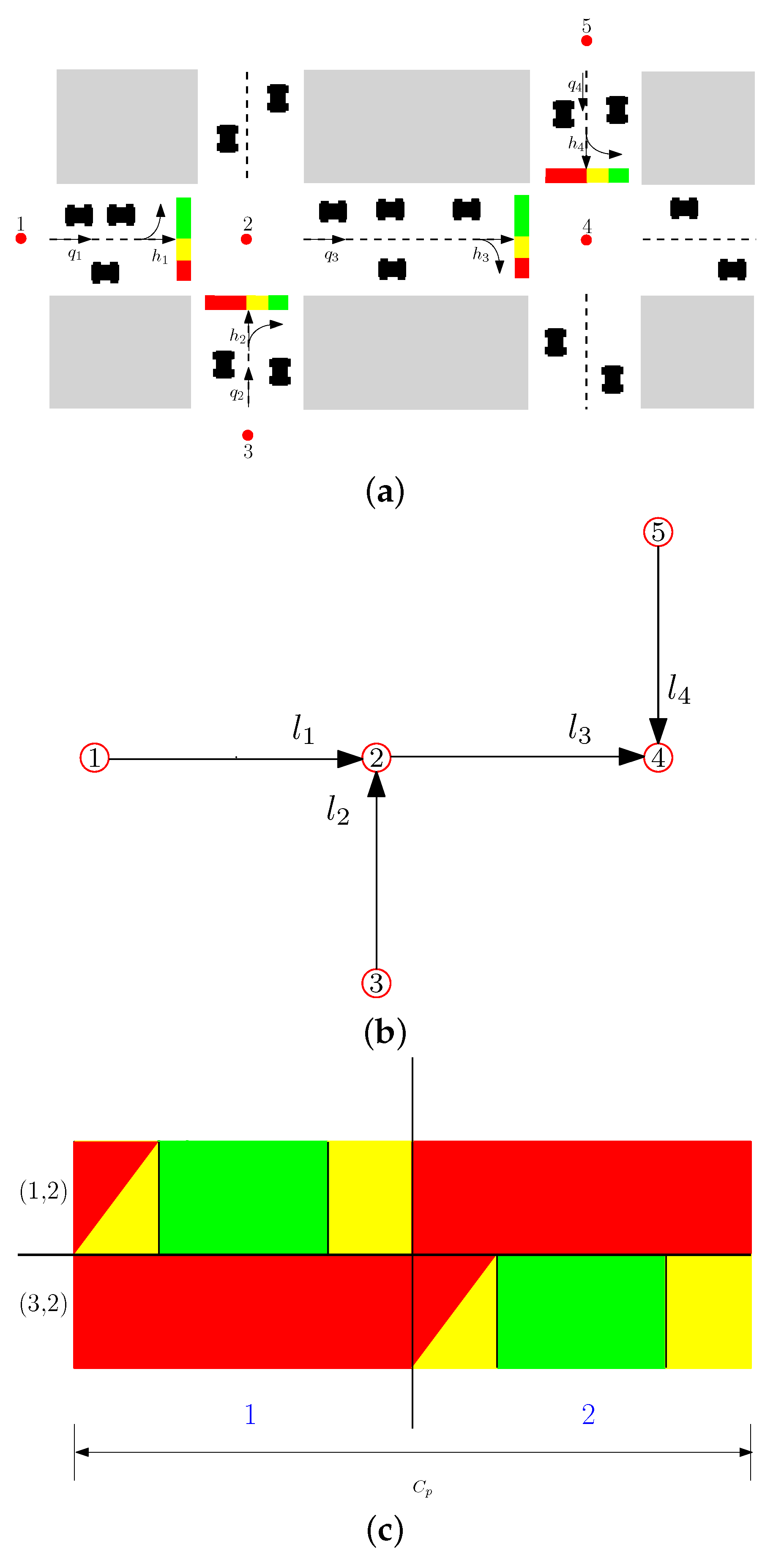
To illustrate this, consider the vehicular traffic network shown in Figure 1a, whose graph representation is shown in Figure 1b, and traffic light behavior described in Figure 1c, where (1,2) represents the link between streets 1 and 2, whereas (3,2) represents the link between streets 3 and 2. The traffic light scheme shows two idle periods in (1,2), one that represents the red–yellow transition, and one that represents the yellow light after the green one. The total idle time is denoted as $L_p$. During the period composed of the idle and green light times in (1,2), the traffic light in (3,2) must be in red. The same scheme applies for (3,2) in the second half of the cycle time $C_p$. Considering the above definitions, the following constraint applies to node p:

$$\sum _{i\in {\mathcal{I}}_p}{g}_i+L_p=C_p,$$

(4)

where $g_i$ is the green light time for link i.

One stage is defined as the time at which an input link to a node p has the right of way (ROW), whereas the set of stages for a node p is denoted as $F_p$. The saturation flow $o_i$, with $i\in {\mathcal{I}}_p$, represents the output vehicular flow capacity for the link i while the traffic light is green. The set of values $\mathbf{o}={\left[o_1,\dots ,o_n\right]}^T$ is normally known as $\forall i\in \mathcal{E}$. The turn rate on each node, denoted by ${\tau }_{\left(i,j\right)}\in \left[0,1\right]$, with $i\in {\mathcal{I}}_p$ and $j\in {\mathcal{O}}_p$, represents the distribution of vehicles turning from link i to j. In other words, ${\tau }_{\left(i,j\right)}$ is the turn rate from link i to j, with $\psi \left(i\right)=\left(p,r\right)$ and $\psi \left(j\right)=\left(l,p\right)$.

The traffic light state in a link $i\in {\mathcal{I}}_p$, denoted as $s_i\in \left\{0,1\right\}$, can be equal to 1 when the traffic light is green (ROW) and 0 in a different case (yellow or red). In general, the set of network states is $\mathbf{s}={\left[s_1,\dots ,s_n\right]}^T$, $\forall i\in \mathcal{E}$.

The expressions $c_i$ and $w_i$, with $i\in {\mathcal{I}}_p$, represent the external vehicular input flow and the vehicular storing capacity of i, respectively. In general terms, $\mathbf{c}={\left[c_i,\dots ,c_n\right]}^T$, $\Omega =\left[w_i,\dots ,w_n\right]$, and $\forall i\in \mathcal{E}$ represent the vehicular input flows and storing capacity of all the network links.

Network Restrictions. The geometry restriction on each link is given by $0\le l_i\le {\overline{l}}_i$, and the control input restriction is represented as ${\underline{g}}_i\le g_i\le {\overline{g}}_i$, where $l_i$ and ${\overline{l}}_i$ are the current and average queue lengths of link i, respectively, and ${\underline{g}}_i$ is the minimum value in seconds for the green light, which depends on the system properties (e.g., it can be equal to zero when there are no vehicles in link i). Finally, the term ${\overline{g}}_i$ represents the addition of all green times in intersection p and is given by ${\overline{g}}_i={\displaystyle \sum _{i\in {\mathcal{I}}_p}}{g}_i\le C_p-L_p$. Observe that this value must not exceed the difference between the cycle time and the total idle time.

3.1. Continuous Modeling of a Urban Traffic Network

The vehicular storing change in a link $i\in \mathcal{E}$ can be modeled as a mass balance, given by

$$w_i{\dot{l}}_i=c_i+q_i-h_i,with{\mathcal{I}}_p\ne \left\{\varphi \right\},$$

(5)

where $h_i$ and ${\dot{l}}_i$ represent the queue output flow and queue length changes, respectively. The input flow change $q_i$ is given by

$$\begin{array}{c}\hfill q_i=\sum _{\begin{array}{c}j\in {\mathcal{I}}_p\end{array}}{\tau }_{\left(j,i\right)}{h}_j,\end{array}$$

(6)

with ${\tau }_{\left(j,i\right)}$ being the turn rate from the input link $j\in {\mathcal{I}}_p$ to node $p\in \mathcal{V}$ direct towards the output link $i\in {\mathcal{O}}_p$. Using (6) and (5), we have

$$\begin{array}{c}\hfill w_i{\dot{l}}_i=c_i+\sum _{j\in {\mathcal{I}}_p}{\tau }_{\left(j,i\right)}{h}_j-h_i.\end{array}$$

(7)

The output traffic flow change of link i is modeled as

$$\begin{array}{c}\hfill \begin{array}{cccccc}{\dot{h}}_i& =& o_i-h_i\hfill & if{s}_i& =& 1,\\ h_i& =& 0\hfill & if{s}_i& =& 0,\end{array}\end{array}$$

(8)

i.e., the traffic flow change is given by the difference between the output vehicular flow capacity for link i while the traffic light is green (saturation flow $o_i$), and the queue output flow change is $h_i$.

Additionally, the green time variation ${\dot{g}}_i$ is expressed as

$$\begin{array}{c}\hfill \begin{array}{cccccc}{\dot{g}}_i& =& 1& if{s}_i& =& 1,\\ g_i& =& 0& if{s}_i& =& 0,\end{array}\end{array}$$

(9)

which is constant when the traffic light state $s_i$ is equal to 1 (green time), since the green time $g_i$ increases linearly from its minimum value ${\underline{g}}_i$ to its maximum value ${\overline{g}}_i$. The second term in (9) indicates that there is no green time variation if the traffic light state $s_i$ is equal to 0 (yellow or red).

Finally, considering (7)–(9) and a $n=\left|\mathcal{E}\right|$ link network, we can represent the system as the differential-algebraic system of equations (DAE) $E_{\sigma }\dot{\xi }=A_{\sigma }\xi +B_{\sigma }$, with the discontinuous coefficients matrix form

$$\begin{array}{cc}\hfill \left[\begin{array}{ccc}{E}_{\Omega }& 0& 0\\ 0& {\mathbf{s}}_{\sigma }& 0\\ 0& 0& {\mathbf{s}}_{\sigma }\end{array}\right]\left[\begin{array}{c}\dot{\mathbf{x}}\\ \dot{\mathbf{h}}\\ \dot{\mathbf{g}}\end{array}\right]& =\hfill \\ \hfill \left[\begin{array}{ccc}0& A_{\tau }& 0\\ 0& {\widehat{\mathbf{s}}}_{\sigma }& 0\\ 0& 0& {\overline{\mathbf{s}}}_{\sigma }\end{array}\right]\left[\begin{array}{c}\mathbf{x}\\ \mathbf{h}\\ \mathbf{g}\end{array}\right]& +\left[\begin{array}{c}\mathbf{c}\\ {\mathbf{s}}_{\sigma }\mathbf{o}\\ {\mathbf{s}}_{\sigma }^T\end{array}\right]\hfill \end{array},$$

(10)

where ${\mathbf{s}}_{\sigma }=\left[s_1^{*},\dots ,s_n^{*}\right]$ is the network configuration in a given mode $\sigma$. $E_{\Omega }\in {\mathbb{R}}^{n\times n}$ is a diagonal matrix whose elements are the $E_{\Omega }^i=w_i\in \Omega$. ${\overline{s}}_i^{*}=1-s_i^{*}$, and ${\overline{\mathbf{s}}}_{\sigma }=diag\left(\left[{\overline{s}}_1^{*},\dots ,{\overline{s}}_n^{*}\right]\right)$. ${\widehat{s}}_i^{*}=-2s_i^{*}+1$, and ${\widehat{\mathbf{s}}}_{\sigma }^{*}=diag\left(\left[{\widehat{s}}_1^{*},\dots ,{\widehat{s}}_n^{*}\right]\right)$. The matrix $A_{\tau }\in {\mathbb{R}}^{n\times n}$ is built by the proper selection of the turn rates.

Rewriting (10) as an homogeneous system, we have

$$E_{\sigma }\dot{\xi }=A_{\sigma }\xi ,$$

(11)

whose matrix form is

$$\begin{array}{cc}\hfill \left[\begin{array}{cccccc}{E}_{\Omega }& 0& 0& 0& 0& 0\\ 0& {\mathbf{s}}_{\sigma }& 0& 0& 0& 0\\ 0& 0& {\mathbf{s}}_{\sigma }& 0& 0& 0\\ 0& 0& 0& {\mathbf{I}}_n& 0& 0\\ 0& 0& 0& 0& {\mathbf{I}}_n& 0\\ 0& 0& 0& 0& 0& {\mathbf{I}}_n\end{array}\right]\left[\begin{array}{c}\dot{\mathbf{l}}\\ \dot{\mathbf{h}}\\ \dot{\mathbf{g}}\\ \dot{\mathbf{s}}\\ \dot{\mathbf{c}}\\ \dot{\mathbf{o}}\end{array}\right]& =\left[\begin{array}{cccccc}0& A_{\tau }& 0& 0& {\mathbf{I}}_n& 0\\ 0& {\widehat{\mathbf{s}}}_{\sigma }& 0& 0& 0& {\mathbf{s}}_{\sigma }{\mathbf{I}}_n\\ 0& 0& {\overline{\mathbf{s}}}_{\sigma }& {\mathbf{I}}_n& 0& 0\\ 0& 0& 0& 0& 0& 0\\ 0& 0& 0& 0& 0& 0\\ 0& 0& 0& 0& 0& 0\end{array}\right]\left[\begin{array}{c}\mathbf{l}\\ \mathbf{h}\\ \mathbf{g}\\ \mathbf{s}\\ \mathbf{c}\\ \mathbf{o}\end{array}\right].\hfill \end{array}$$

3.2. Hybrid Urban Traffic System

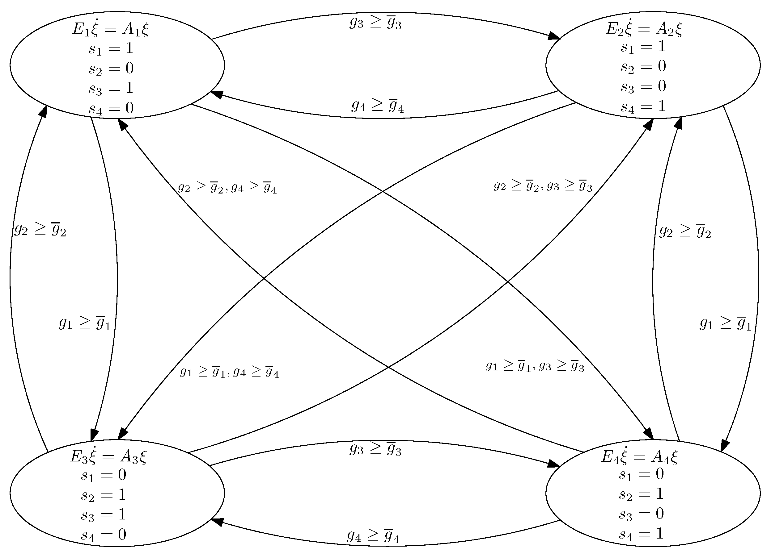
The urban traffic network integrates the continuous scheme described in Section 3.1 with the discrete behavior resulting from transitions between different network modes. This integration allows us to model the network as a hybrid system. To illustrate this, consider the network depicted in Figure 1a and its representation by the automaton in Figure 2. In this case, we have four traffic lights, each one with two possible states $\{0,1\}$, i.e., we have $2^4=16$ possible network configurations. However, since $s_1=\sim s_2$ and $s_3=\sim s_4$, this number can be reduced to $2^2=4$, which is the number of ovals in the automaton. The set of modes is denoted as $\Sigma =\{{\sigma }_1,{\sigma }_2,{\sigma }_3,{\sigma }_4\}$. The transitions between states are governed by a threshold condition based on the difference between the green time of individual links ($g_i$) and the total green time at each node (${\overline{g}}_i$). For instance, the transition from mode ${\sigma }_2=[1,0,0,1]$ to ${\sigma }_1=[1,0,1,0]$ is triggered when $g_4\ge {\overline{g}}_4$, i.e., when the green time in link 4 is greater or equal than the sum of green times of links 3 and 4 (${\overline{g}}_4=g_4+g_3$). In this sense, the switching scheme between modes is dynamic and depends on the variation of green times of links, which changes according to the fitness function used in the control strategies described in Section 4.

In general, the state vector for this system is

$$z=\left(\xi ,\sigma \right)\in {\mathbb{R}}^n\times \Sigma ,$$

where $\Sigma$ is a finite discrete set of modes. The DAE hybrid system representation is

$${\mathcal{H}}_{DAE}\left\{\begin{array}{cc}\left[\begin{array}{cc}{E}_{\sigma }& 0\\ 0& 1\end{array}\right]& \left[\begin{array}{c}\dot{\xi }\\ \dot{\sigma }\end{array}\right]=\left[\begin{array}{c}{f}_{\sigma }\left(\xi \right)\\ 0\end{array}\right]=F\left(z\right),z\in C\\ & \left[\begin{array}{c}{\xi }^{+}\\ {\sigma }^{+}\end{array}\right]\in \left[\begin{array}{c}{\tilde{g}}_{\sigma }\left(\xi \right)\\ {\phi }_{\sigma }\left(\xi \right)\end{array}\right]=G\left(z\right),z\in D\end{array}\right.,$$

where

$$\begin{array}{ccc}\hfill f_{\sigma }\left(\xi \right)& =& A_{\sigma }\xi \hfill \\ \hfill C& =& \bigcup _{\sigma \in \sum }\left(C_{\sigma }\cap {\mathfrak{O}}_{\sigma }\right)\hfill \\ \hfill {\tilde{g}}_{\sigma }\left(\xi \right)& =& g_D\left(z\right)\cup g_{\mathfrak{O}}\left(z\right)\hfill \\ \hfill D& =& \bigcup _{\sigma \in \sum }\left(\left(D_{\sigma }\cap {\mathfrak{O}}_{\sigma }\right)\cup \left(\left({\mathbb{R}}^n\times \left\{\sigma \right\}\right)\setminus {\mathfrak{O}}_{\sigma }\right)\right)\hfill \end{array}$$

and

$$\begin{array}{ccc}\hfill g_D\left(z\right)& =& \left\{\begin{array}{ccc}\prod _{\phi \sigma \left(\xi \right)}{g}_{\sigma }\left(\xi \right)& & ifz\in D_{\sigma }\cap {\mathfrak{O}}_{\sigma }\\ 0& & otherwise\end{array}\right.\hfill \end{array}$$

$$\begin{array}{ccc}\hfill g_{\mathfrak{O}}\left(z\right)& =& \left\{\begin{array}{ccc}\prod _{\phi \sigma \left(\xi \right)}\xi & & ifz\in \left({\mathbb{R}}^n\times \left\{\sigma \right\}\right)\setminus {\mathfrak{O}}_{\sigma }\\ 0& & otherwise\end{array}\right.\hfill \end{array}$$

${\mathfrak{O}}_{\sigma }$ and ${\prod }_{\sigma }$ represent the consistency sets and the projectors, respectively [29]. $C_{\sigma }=\left\{z:g_i\in \left[0,{\overline{g}}_i\right],\mathbf{s}=\left[s_1,\dots ,s_n\right],\sigma \in \sum \right\}$, and $D_{\sigma }=\left\{z:g_i\ge {\overline{g}}_i,\mathbf{s}=\left[s_1,\dots ,s_n\right],\sigma \in \sum \right\}$ are subsets $\in {\mathbb{R}}^n$ that define the system evolution according to F and G. In the transitions between modes, the changes of $\xi$ are defined by the map $g_{\sigma }\left(\xi \right)={\left[\mathbf{l},\mathbf{h},y_{\mathbf{g}}\left(\mathbf{g}\right),y_{\mathbf{s}}\left(\mathbf{g},\sigma \right),\mathbf{c},\mathbf{o}\right]}^T$, where

$$y_{\mathbf{g}}\left(\mathbf{g}\right)=\begin{array}{c}\left\{{\left[g_1,\dots ,g_n\right]}^T:g_i\left\{\begin{array}{ccccc}{g}_i& if& g_i& \le & {\overline{g}}_i\\ 0& if& g_i& \ge & {\overline{g}}_i\\ g_i,0& if& g_i& =& {\overline{g}}_i\end{array}\right.\right\}\end{array}$$

and

$$y_{\mathbf{s}}\left(\mathbf{g},\sigma \right)=\left\{{\left[s_1,\dots ,s_n\right]}^T\begin{array}{cc}:& g_i\ge {\overline{g}}_i,\end{array}\sigma \in \sum \right\}.$$

Additionally, the changes of modes in the network are determined by

$${\phi }_{\sigma }\left(\xi \right)=\left\{\begin{array}{cc}\sigma :& g_i\ge {\overline{g}}_i,\sigma \in \sum \end{array}\right\}.$$

4. Population Game-Based Model for Urban Traffic Control

In the urban traffic system, each node $p\in \mathcal{V}:{\mathcal{I}}_p\ne \varphi$ is represented as a population of agents that share the effective green time $m={\sum }_{i\in {\mathcal{I}}_p}{g}_i$. In this sense, agents form a mass m distributed between the set of pure strategies $S=\left\{1,\dots ,\mathrm{n}\right\}$ of the population. The set S, corresponds to the set of stages $F_p$ described in Section 3, i.e., the proportion of m that the input links of node p have for the right of way (ROW). Thus, each link $j\in {\mathcal{I}}_p$ is assigned a proportion $x_j$ of m, which is a pure strategy of the population.

The whole behavior of the agents defines the population state x, which belongs to the simplex

$$\Delta =\{x\in {\mathbb{R}}_{+}^{\mathrm{n}}:\sum _{\mathrm{j}\in S}{x}_{\mathrm{j}}=m\}.$$

(12)

The set of agents assuming a strategy $j\in S$ allows us to obtain a payoff provided by the fitness function $F_{\mathrm{j}}\left(x\right):\Delta \to \mathbb{R}$, in a determined population state x. The average fitness function is defined as $\overline{F}\left(x\right)={\displaystyle \frac{1}{m}}{\displaystyle \sum _{\mathrm{j}\in S}}{x}_{\mathrm{j}}{F}_{\mathrm{j}}\left(x\right)$, and the excess payoff of j is ${\widehat{F}}_j\left(x\right)=F_{\mathrm{j}}\left(x\right)-\overline{F}\left(x\right)$.

In this approach, the fitness function for a given link j is the relation between its queue length and its assigned proportion of m. This lead us to Definition 1.

Definition 1. 

The fitness function for the adaptive control strategies based in population games depends on the relation between the link queue capacity and its green time assignment. This is given by

$$F_{\mathrm{j}}\left(x\right)={\displaystyle \frac{l_{\mathrm{j}}}{x_{\mathrm{j}}}},$$

(13)

which must be minimized.

4.1. Mean Dynamics and Revision Protocols

In mean dynamics, each of the n agents receive equally likely revision opportunities at rate R, which means that agents playing strategy j have an expected number of opportunities given by $n{x}_{j}Rdt$ in a time space $dt$ to observe their opponents behavior in order to make decisions. On the other hand, the expected number of opportunities that the agents have to change from strategy j to k is $n{x}_j{\rho }_{jk}\left(x\right)dt$, where ${\rho }_{jk}$ represents the conditional switch rate to change from j to k. In this way, the expected change of agents using strategy j is given by

$$\left(\sum _{\mathrm{k}\in S}{x}_{\mathrm{k}}{\rho }_{\mathrm{k}\mathrm{j}}-x_{\mathrm{j}}\sum _{\mathrm{k}\in S}{\rho }_{\mathrm{j}\mathrm{k}}\right)dt,$$

(14)

from which we define an expected-value-based dynamic known as the mean dynamic, given by

$${\dot{x}}_j=\sum _{\mathrm{k}\in S}{x}_{\mathrm{k}}{\rho }_{\mathrm{k}\mathrm{j}}-x_{\mathrm{j}}\sum _{\mathrm{k}\in S}{\rho }_{\mathrm{j}\mathrm{k}}.$$

(15)

The above expression determines how the proportion of agents playing strategy j varies [30].

The switch change ${\rho }_{jk}$ also defines the revision protocols shown in

Table 1. Revision protocols and switch rates.

Revision Protocol	Function
Pairwise proportional imitation	${\rho }_{\mathrm{j}\mathrm{k}}=x_{\mathrm{k}}{\left[F_{\mathrm{k}}-F_{\mathrm{j}}\right]}_{+}$
Pairwise comparison	${\rho }_{\mathrm{j}\mathrm{k}}={\left[F_{\mathrm{k}}-F_{\mathrm{j}}\right]}_{+}$
Logit selection	${\rho }_{\mathrm{j}\mathrm{k}}={\displaystyle \frac{exp\left({\eta }^{-1}{F}_{\mathrm{k}}\right)}{{\displaystyle \sum _{\mathrm{w}\in S}}exp\left({\eta }^{-1}{F}_{\mathrm{w}}\right)}}$
Comparison with average utility	${\rho }_{\mathrm{j}\mathrm{k}}={\left[F_{\mathrm{k}}-{\displaystyle \sum _{\mathrm{w}\in S}}{x}_{\mathrm{w}}{F}_{\mathrm{w}}\right]}_{+}$

. These revision protocols determine the population dynamic used by the agent population. We describe them in detail in Section 4.2, with a particular focus on the fictitious play case, since it uses historical data to define agent strategies, demonstrating its viability within a fixed-time traffic framework.

4.2. Population Dynamics

In this section, we describe the population dynamics employed in this approach to optimize the green times for each node in the traffic network. First, we describe the dynamics that, due to their online nature, are used for adaptive control strategies. These dynamics are replicator, Brown–Von Neuman–Nash, Logit and Smith, which use (13) as a fitness function. Subsequently, we describe fictitious play as a fixed-time control strategy, since it uses historical data for agent decision making. In this case, the payoff function is given by (22).

4.2.1. Replicator Dynamics

The replicator dynamic (RD) describes how the frequencies of different strategies change over time based on the fitness associated with each one, i.e., strategies having higher payoffs tend to increase in frequency within the population, while less successful strategies decrease. An agent using this type of dynamics chooses an opponent and applies the imitation protocol. The opponent’s strategy is followed by this when its utility is better than the current one. This dynamic is described as the difference between the fitness of the strategy j and the average fitness, as follows:

$${\dot{x}}_{\mathrm{j}}=x_{\mathrm{j}}\left[F_{\mathrm{j}}\left(x\right)-\overline{F}\left(x\right)\right].$$

(16)

4.2.2. Brown–Von Neumann–Nash

The Brown–Von Neumann–Nash (BNN) dynamic relies on the excess payoff dynamic, since it compares the excess payoff of strategy j with the excess payoff caused by the switch from strategy j to k. It can be expressed as

$${\dot{x}}_{\mathrm{j}}={\left[{\widehat{F}}_{\mathrm{j}}\left(x\right)\right]}_{+}-x_{\mathrm{j}}\sum _{\mathrm{k}\in S}{\left[{\widehat{F}}_{\mathrm{k}}\left(x\right)\right]}_{+}.$$

(17)

4.2.3. Logit Dynamic

The Logit dynamic adopts the Gibbs–Boltzmann form of (18), in which the rationality parameter $\beta$ is included to increase the probability of strategies having better payoffs or to assign them the same probability to be chosen. In the first case, when $\beta \to \infty$, agents play following the best response rule, and in the second case, when $\beta \approx 0$, agents play under a uniform distribution scheme to select strategies.

$$\begin{array}{c}\hfill {\dot{x}}_{\mathrm{j}}={\displaystyle \frac{exp\left(\beta F_{\mathrm{j}}\left(x\right)\right)}{{\displaystyle \sum _{\mathrm{j}\in S}}exp\left(\beta F_{\mathrm{j}}\left(x\right)\right)}}-x_{\mathrm{j}}\end{array}$$

(18)

Rationality $\beta$ can be interpreted as the inverse of the noise $\eta$, and it is included in the Logit selection protocol shown in Table 1.

4.2.4. Smith Dynamic

In Smith dynamics, agents randomly select a strategy and evaluate its payoff against the current strategy. If the new payoff surpasses the current one, the agent switches to the new strategy with a probability proportional to the difference between the payoffs. Unlike the BNN dynamic, which carries out a comparison against the average payoff, or RD, which compares against an opponent strategy, the Smith dynamic involves a direct comparison between two strategies, which avoids some strategies being eventually discarded. This dynamic is described by

$$\begin{array}{c}\hfill {\dot{x}}_{\mathrm{j}}=\sum _{\mathrm{k}\in S}{x}_{\mathrm{k}}{\left[F_{\mathrm{j}}\left(x\right)-F_{\mathrm{k}}\left(x\right)\right]}_{+}-x_{\mathrm{j}}\sum _{\mathrm{k}\in S}{\left[F_{\mathrm{k}}\left(x\right)-F_{\mathrm{j}}\left(x\right)\right]}_{+}\end{array}$$

(19)

4.3. Fictitious Play

In fictitious play, a player i plays a pure best response (BR) action $a_i$ based on the joint distribution of the selected actions of its opponents. This can be expressed by

$$a_i^t\in B{R}_i\left({\mathbf{p}}_{\_\mathbf{i}}^{\mathbf{t}}\right),$$

(20)

where $a_i^t$ represents the action performed by agent i at time t, and ${\mathbf{p}}_{\_\mathbf{i}}^{\mathbf{t}}$ is the joint probability distribution of actions performed by all players except i. The marginal probability for each player i up to time t is calculated using the expression

$$p_i^t={\displaystyle \frac{{\gamma }_i^t\left(a_i\right)}{t}},$$

(21)

where ${\gamma }_i^t\left(a_i\right)={\sum }_{\tau =0}^{t-1}\mathcal{I}\{a_i^{\tau }=a_i\}$ is an S-dimensional vector that counts the times that player i has played each action. According to the above expressions, it is noticeable that in fictitious play, each agent requires historical data in order to make decisions. Consequently, in our context, this control strategy is assumed to follow a fixed-time approach.

The payoff for an agent i is a function that depends on its current action and the action set $a_{\_i}$ played by the agents different to i. In our case, this payoff depends on the queue length of links converging to a node. This is presented in Definition 2.

Definition 2. 

The payoff function in a fixed-time scheme modeled as a fictitious play based-control strategy depends on the accumulative queue length of the incidents links. This is given by

$$U(a_i,a_{\_i})=\stackrel{n}{\sum _{i=1}}{l}_i,$$

(22)

which must be minimized.

According to Definitions 1 and 2, fitness and payoff functions determine the control strategies’ dynamics in adaptive and fixed-time schemes, respectively. For the adaptive control case, given by the online population dynamics described in Section 4.2, the green time is continuously updated according to the fitness function variation, which impacts the transition between the modes of the hybrid system described in Section 3.2. In the fixed-time case, the payoff function depends exclusively on the queue lengths of incident links to a specific node, which means that the mode transitions are determined by the current network configuration and the modes that have provided the best queue length reduction historically.

Both functions are strongly related with the traffic network dynamics for which they were taught, i.e., to associate good fitness or payoffs in links with low queue lengths and acceptable green times. The results of the dynamic changes in the functions’ values are described through the performance parameters for different scenarios, as shown in Section 7.

5. Traffic Simulator

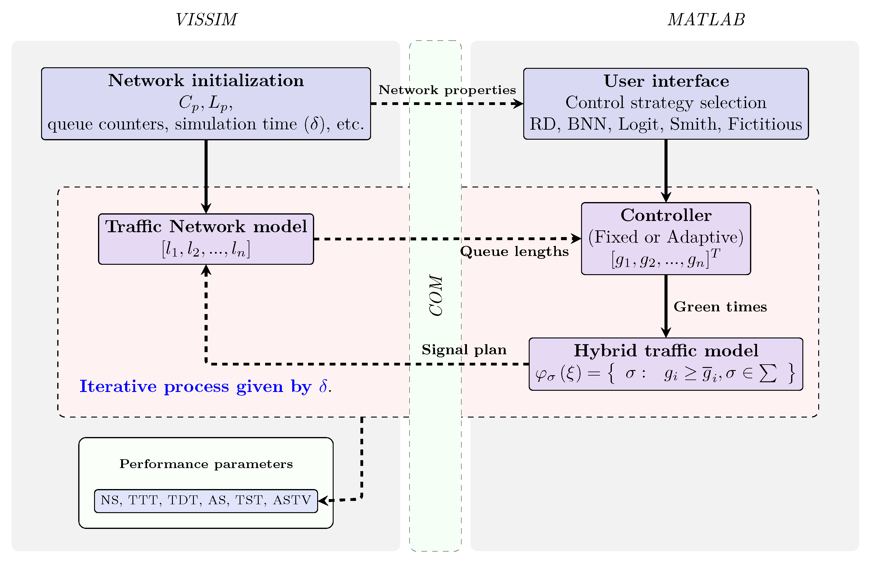
The implemented traffic simulator is shown in Figure 3. This integrates, through a COM server, the VISSIM platform, in which the traffic network is implemented, and MATLAB, where the control strategies described in Section 4.1 and the hybrid model described in Section 3.2 are implemented.

The following are the main steps in the information flow between both simulator sections:

• First of all, the vehicular traffic network is implemented in VISSIM. Subsequently, MATLAB obtains all its properties, such as number of controllers, traffic lights, queue counters, number of links, cycle time ($C_p$), duration of yellow and red lights (intermediate times), and simulation time, among others.
• The runtime environment, which is implemented in an object-oriented scheme, allows for the creation of class instances that represent the traffic network (implemented in VISSIM) and the virtual traffic controller associated with each node that is modeled by means of the hybrid dynamics described in Section 3.2.
• The initial green times are loaded through class instances that represent the control strategies described in Section 4.1. These times, along with the cycle time ($C_p$) and the intermediate times (red and yellow), are used to generate the signaling plan for each controller, which is sent to VISSIM.
• The update of the signaling plan, as well as the reading of the queue counters, are made in sample intervals $\delta$. After this time, the queue lengths calculated in VISSIM are sent to the control strategy instance in order to recalculate the green times. This process is repeated until the simulation time expires.
• Finally, the communication between both modules ends and the information related to performance parameters is stored in VISSIM.

VISSIM includes a COM programming module that allows for an interaction with external programming languages and platforms such as MATLAB in a stable form. In our case, the traffic simulator architecture has an object-oriented scheme implemented in MATLAB, whose main classes are the following:

• COMInterfaceVISSIM: Builds the VISSIM and MATLAB COM connection. It also contains methods to send information to VISSIM (cycle time, simulation time, performance parameters to be measured, etc).
• HybridController: Each instance of this class creates a “virtual controller” that interprets the signal plans and sends the instructions that the VISSIM controllers must follow.
• ControllerUserDefined: Used to define the control strategy to be used. It also generates the green times for each virtual controller generated.
• SignalPlan: Creates the signal plans from the information provided in the graphic interface and the green times given by ControllerUserDefined.
• MainSimulation: Main class in which the instances of the previously described classes are created.

6. Case Study

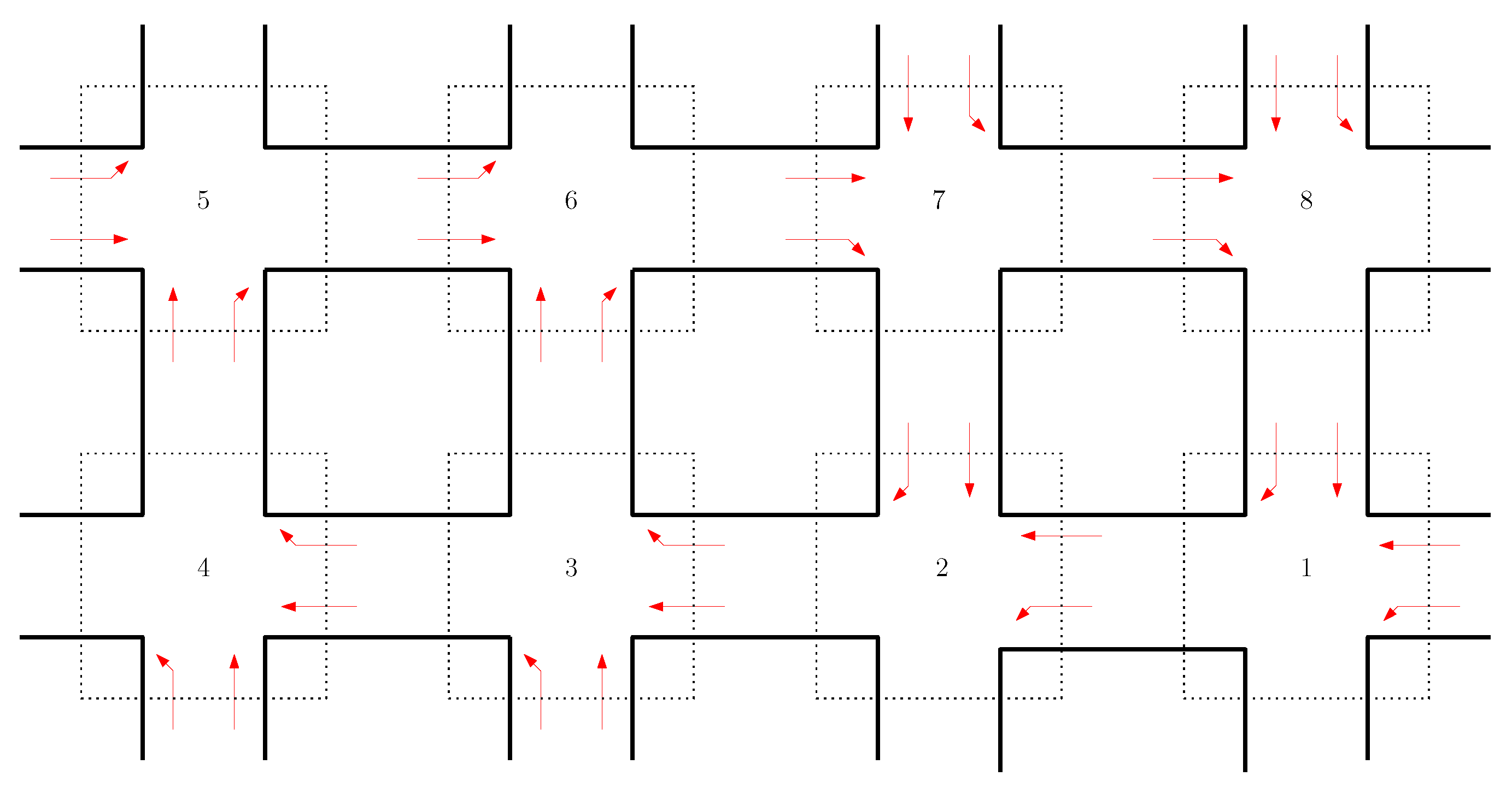
Figure 4 shows the geometry and movement scheme for the traffic network used as a case study, which is located in the urban zone of Barranquilla city in Colombia (between 82 and 84 streets, and Kra. 50 to Kra. 52). The current traffic plans, which are based on a fixed-time strategy that considers only the queue length and historical data, were provided by the city traffic controller company (IMATIC). The results shown in Section 7, compare its performance with the proposed game theory-based controllers for multiple network parameters. In particular, this network has a reduced space between nodes, which avoids a large amount of vehicles within links. The number of input links for each node is 2, which is associated with the number of strategies that each agent can assume in the current node. In general, 16 links are modeled in this approach. Since the network is continuously changing. Moreover, with the aim to test the different control strategies provided by the population dynamics described in Section 4.2, we propose the five scenarios described in

Table 2. Simulation scenarios.

Scenario	Name	Description
1	No saturation condition 1	The input flow of vehicles is constant and equal to $1000{\displaystyle \frac{veh}{h}}$ during the simulation.
2	No saturation condition 2	Input flow increased to $1600{\displaystyle \frac{veh}{h}}$ during the simulation.
3 1	Saturation condition 1	Horizontal links (Streets 82 and 84) are saturated with input flows of $2400{\displaystyle \frac{veh}{h}}$. Additionally, vertical links have flows of $1400{\displaystyle \frac{veh}{h}}$. These values are constant during the simulation time.
4	Saturation condition 2	Vertical links (Kras. 50 to 52) are saturated with input flows of $2000{\displaystyle \frac{veh}{h}}$. Additionally, streets (horizontal links) have flows of $1000{\displaystyle \frac{veh}{h}}$. These values are constant during the simulation time.
5	Variable conditions	Flows for horizontal and vertical links change during the simulation time

¹ The saturation flow rate of 2400 vehicles/hour is a parameter that has been reported in multiple works related to traffic analysis, mostly using a passenger car as a standard unit [31,32,33].

.

7. Discussion

The implemented control strategies based on the population dynamics described in Section 4.1 were used on each one of the scenarios described in Table 2, during a simulation time of $3600s$, with sample intervals $\delta =5s$, cycle time $C_p=60s$ and idle time $L_p=10s$.

The performance of each control strategy is evaluated according to the parameters shown in

Table 3. Performance parameters.

Parameter	Description
NS	Number of Stops
TTT	Total Travel Time
TDT	Total Distance Traveled
AS	Average Speed
TST	Total Stop Time
ASTV	Average Stop Time per Vehicle

and compared in

Table 4. Performance parameters for control strategies.

Scenario	Controller	NS[veh]	TTT[h]	TDT[km]	AS[km/h]	TST[seg]	ASTV[h]
	FP	7917$\left(-6\%\right)$	183.1$\left(-3\%\right)$	8526.2$\left(0.1\%\right)$	46.6$\left(3.3\%\right)$	13.7$\left(-11\%\right)$	22.6$\left(-11\%\right)$
	RD	8257$\left(-2\%\right)$	188.1$\left(-0.4\%\right)$	8522.3$\left(0.1\%\right)$	45.3$\left(0.4\%\right)$	15.9$\left(3\%\right)$	26.1$\left(3\%\right)$
1	BNN	8618 $\left(2\%\right)$	188.9$\left(0.1\%\right)$	8568.8$\left(0.6\%\right)$	45.4$\left(0.7\%\right)$	15.4$\left(0\%\right)$	25.4$\left(0\%\right)$
	Smith	7803$\left(-8\%\right)$	181.9$\left(-4\%\right)$	8491.7$\left(-0.3\%\right)$	46.7$\left(3.5\%\right)$	13.6$\left(-12\%\right)$	22.4$\left(-11\%\right)$
	Logit$\left(\eta =1\right)$	8699$\left(3\%\right)$	189.9$\left(0.6\%\right)$	8558.3$\left(0.5\%\right)$	45.1$\left(0\%\right)$	15.8$\left(3\%\right)$	26.0$\left(3\%\right)$
	FP	16,941$\left(-71\%\right)$	331.5$\left(-18\%\right)$	13,557.1$\left(1\%\right)$	40.9$\left(23\%\right)$	18.1$\left(-29\%\right)$	47.9$\left(-29\%\right)$
	RD	15,321$\left(-74\%\right)$	318.8$\left(-21\%\right)$	13,496.4$\left(1\%\right)$	42.3$\left(27\%\right)$	16.24$\left(-37\%\right)$	42.9$\left(-36\%\right)$
2	BNN	17,870$\left(-70\%\right)$	337.4$\left(-16\%\right)$	13,569.9$\left(1\%\right)$	40.2$\left(21\%\right)$	18.9$\left(-26\%\right)$	50.0$\left(-26\%\right)$
	Smith	15,608$\left(-74\%\right)$	320.7$\left(-20\%\right)$	13,537.8$\left(1\%\right)$	42.2$\left(27\%\right)$	16.0$\left(-38\%\right)$	42.3$\left(-37\%\right)$
	Logit$\left(\eta =1\right)$	17,885$\left(-70\%\right)$	337.7$\left(-16\%\right)$	13,570.6$\left(1\%\right)$	40.2$\left(21\%\right)$	18.9$\left(-26\%\right)$	49.8$\left(-26\%\right)$
	FP	56,974$\left(-17\%\right)$	452.1$\left(-6\%\right)$	14,377.1$\left(6\%\right)$	31.8$\left(13\%\right)$	24.7$\left(11\%\right)$	70.2$\left(18\%\right)$
	RD	52,301$\left(-24\%\right)$	456.7$\left(-5\%\right)$	14,209.7$\left(5\%\right)$	31.1$\left(10\%\right)$	19.6$\left(-12\%\right)$	55.7$\left(-7\%\right)$
3	BNN	67,506$\left(-1\%\right)$	470.3$\left(-2\%\right)$	13,624.5$\left(1\%\right)$	29.0$\left(3\%\right)$	20.7$\left(-7\%\right)$	56.2$\left(-6\%\right)$
	Smith	54,569$\left(-20\%\right)$	458.5$\left(-4\%\right)$	14,185.8$\left(5\%\right)$	30.9$\left(10\%\right)$	19.5$\left(-12\%\right)$	54.9$\left(-8\%\right)$
	Logit$\left(\eta =1\right)$	67,158$\left(-2\%\right)$	471.6$\left(-2\%\right)$	13,620.6$\left(1\%\right)$	28.9$\left(2\%\right)$	20.9$\left(-6\%\right)$	56.4$\left(-6\%\right)$
	FP	21,087$\left(-88\%\right)$	367.4$\left(-32\%\right)$	14,164.8$\left(17\%\right)$	38.6$\left(72\%\right)$	19.2$\left(-43\%\right)$	52.9$\left(-35\%\right)$
	RD	19,087$\left(-90\%\right)$	353.4$\left(-34\%\right)$	14,192.7$\left(17\%\right)$	40.2$\left(79\%\right)$	17.2$\left(-49\%\right)$	47.4$\left(-42\%\right)$
4	BNN	51,206$\left(-72\%\right)$	432.9$\left(-20\%\right)$	14,106.1$\left(17\%\right)$	32.4$\left(44\%\right)$	23.1$\left(-32\%\right)$	63.4$\left(-22\%\right)$
	Smith	18,407$\left(-90\%\right)$	350.3$\left(-35\%\right)$	14,166.2$\left(17\%\right)$	40.4$\left(80\%\right)$	17.0$\left(-50\%\right)$	46.9$\left(-43\%\right)$
	Logit $\left(\eta =1\right)$	59,657$\left(-67\%\right)$	450.8$\left(-16\%\right)$	14,041.3$\left(16\%\right)$	31.1$\left(38\%\right)$	24.0$\left(-29\%\right)$	65.9$\left(-19\%\right)$
	FP	52,650$\left(-53\%\right)$	419.5$\left(-13\%\right)$	13,823.6$\left(7\%\right)$	32.9$\left(23\%\right)$	21.9$\left(-20\%\right)$	60.7$\left(-14\%\right)$
	RD	25,001$\left(-77\%\right)$	367.6$\left(-24\%\right)$	14,206.7$\left(10\%\right)$	38.6$\left(44\%\right)$	18.3$\left(-33\%\right)$	51.4$\left(-28\%\right)$
5	BNN	50,421$\left(-55\%\right)$	430.9$\left(-11\%\right)$	13,978.1$\left(8\%\right)$	32.4$\left(21\%\right)$	22.0$\left(-20\%\right)$	61.3$\left(-14\%\right)$
	Smith	22,758$\left(-80\%\right)$	363.0$\left(-25\%\right)$	14,232.5$\left(10\%\right)$	39.2$\left(46\%\right)$	18.1$\left(-34\%\right)$	50.8$\left(-28\%\right)$
	Logit$\left(\eta =1\right)$	54,132$\left(-51\%\right)$	435.1$\left(-10\%\right)$	13,940.7$\left(8\%\right)$	32.0$\left(19\%\right)$	21.9$\left(-20\%\right)$	60.9$\left(-14\%\right)$

, with the current fixed-time strategy used by the traffic controller company of Barranquilla city. Observe how most of the proposed control strategies outperform the current one, achieving reductions in the number of stops (NS) up to 90% and increasing the average speed (AS) up to 79% and 80% in scenario 4 with RD and Smith dynamics, respectively. There is not a notable improvement for scenario 1 due to the low and constant flow of vehicles. However, it is noticeable that under saturation and variable conditions, the proposed strategies enhance the results for the evaluated parameters, except the total distance traveled (TDT), which has increased up to 17% in scenario 4 in almost all the proposed strategies. This can be attributed to the change of routes inherent to the dynamics of the strategies.

Another important comparison provided by Table 4 encompasses game theory-based control strategies. In general, both Smith and replicator dynamics demonstrate superior performance in saturated and non-saturated scenarios due to their decentralized mechanisms. In replicator dynamics (RD), agents adjust their strategies based on pairwise fitness comparisons, whereas in Smith dynamics, they compare the expected payoffs of different strategies. This localized decision-making approach eliminates the need for complete information—unlike BNN or Logit dynamics—enhancing adaptability to unpredictable environments and, consequently, traffic volatility.

• Scenario 1.

In this case, the control strategy with better performance was Smith dynamics. As shown in Table 4, all parameters show the most favorable values in comparison with the other controllers. On the other hand, the fixed-time control strategy, fictitious play, demonstrates that is also a good option, with values that do not deviate significantly from the Smith case; Logit ($\eta =1$) yields the least favorable outcomes.

• Scenario 2.

In this scenario, all the control strategies demonstrate a notable improvement in comparison with scenario 1, especially Smith and replicator dynamics. However, there are some parameters in which some control strategies exhibit better behaviour, since Smith dynamics surpasses replicator dynamics in ASTV and TST, whereas the replicator dynamic outperforms the Smith dynamic in TTT.

• Scenario 3.

In this case, the fixed-time strategy, fictitious play, yields superior outcomes compared to the adaptive strategies, replicator and Smith, in certain parameters such as TTT and AS. However, in terms of TST and ASTV, fictitious play is surpassed by them. Once more, the Smith dynamic and replicator demonstrate superior performance, with the replicator dynamic outperforming it in NS and TTT, while Smith dynamics slightly surpass replicator dynamics in TST.

• Scenario 4.

Saturated network conditions are maintained but this time with a reduction in flows in relation to scenario 3. The adaptive strategy, Smith, exhibits the best performance among all strategies, followed by replicator dynamics. The fixed-time strategy based on fictitious play presents better results compared to the BNN and Logit cases.

• Scenario 5.

This last scenario pretends to test the adaptive strategies’ performance. Again, the best results are obtained for Smith and replicator dynamics, in that order. Since this scenario is completely variable, the fixed-time strategy, fictitious play, exhibits a performance reduction in comparison with BNN and Logit, in relation to scenario 4.

8. Conclusions

In this work, we implemented a traffic simulator that combines the micro-simulation platforms VISSIM and MATLAB in order to include population game-based control strategies to define green times in an eight-intersection traffic network. Due to its determinant role in network congestion, the queue length of links is an important parameter for fitness and payoff functions’ definitions, both in the fixed case, which is modeled using fictitious play dynamics, and for the adaptive case, modeled using the control strategies based on RD, BNN, Logit and Smith dynamics. Within the traffic simulator, we included a hybrid system to model both the continuous and discrete behavior of the network in order to involve both the vehicular storing change in links and the transitions between modes caused by the traffic light changes in nodes. The results, obtained in five different traffic scenarios, demonstrated acceptable performance for the fixed-time scheme modeled with fictitious play in a traffic network without saturation conditions. In conditions considering saturation and variability in traffic flows, fictitious play exhibited good performance in many of the analyzed parameters, specifically in NS, TTT, AS, TST and ASTV, in which it outperformed BNN and Logit dynamics. On the other hand, Smith dynamics emerged as the most effective control strategy across all studied scenarios, consistently outperforming the others, particularly in situations where increased congestion led to a decline in fitness values. Replicator dynamics also demonstrated strong performance, though slightly behind Smith dynamics. This superior performance can be attributed to the decentralized nature of Smith dynamics and RD. In the case of RD, agents adjust their strategies based on pairwise comparisons of fitness values, while in Smith dynamics, agents compare the expected payoffs of different strategies. This localized decision-making process enhances their adaptability in unpredictable environments, such as traffic conditions, as they do not rely on a complete information scheme, which is a requirement that other dynamics, such as BNN or Logit, depend on.

The proposed model, unlike other related works, considers five distinct levels of saturation or traffic characteristics, ranging from constant flows to variable flows in both vertical and horizontal links. Under these scenarios, the performance of various control strategies based on game theory was evaluated across multiple parameters, including the number of stops (NS), total travel time (TTT), total distance traveled (TDT), average speed (AS), total stop time (TST), and average stop time per vehicle (ASTV). Although the density of traffic flows can be adjusted to further validate the results, this study demonstrates that certain control strategies outperform others across most performance metrics, particularly under high saturation levels. The findings provide clear evidence of which game theory-based control strategies are best-suited for fixed or adaptive schemes. Furthermore, the traffic network is modeled as a hybrid system, a novel approach not explored in previous studies. This hybrid modeling provides a more realistic representation of traffic behavior, capturing both the continuous and discrete dynamics inherent in real-world traffic systems.

Limitations and Future Directions

Although VISSIM and MATLAB are widely used for traffic analysis, the proposed combination operates in a simulated environment that accounts for various congestion conditions and performance metrics. However, it does not incorporate real-world data, which would enhance the accuracy and practical applicability of the results. Therefore, future research should focus on implementing this approach using actual traffic datasets and more complex traffic networks. Additionally, it is important to consider how the proposed control strategies could improve the performance in terms of the TDT parameter, which was the only one presenting negative behavior in saturated scenarios.