Niching-Driven Divide-and-Conquer Hill Exploration

Abstract

Optimization problems often feature local optima with a significant difference in the basin of attraction (BoA), making evolutionary computation methods prone to discarding solutions located in less-attractive BoAs, thereby posing challenges to the search for optima in these BoAs. To enhance the ability to find these optima, various niching methods have been proposed to restrict the competition scope of individuals to their specific neighborhoods. However, redundant searches in more-attractive BoAs as well as necessary searches in less-attractive BoAs can only be promoted simultaneously by these methods. To address this issue, we propose a general framework for niching methods named niching-driven divide-and-conquer hill exploration (NDDCHE). Through gradually learning BoAs from the search results of a niching method and dividing the problem into subproblems with a much smaller number of optima, NDDCHE aims to bring a more balanced distribution of searches in the BoAs of optima found so far, and thus enhance the niching method’s ability to find optima in less-attractive BoAs. Through experiments where niching methods with different categories of niching techniques are integrated with NDDCHE and tested on problems with significant differences in the size of the BoA, the effectiveness and the generalization ability of NDDCHE are proven.

1. Introduction

Many optimization problems have a large number of local optima. To locate the desired optima—normally the global ones—a variety of evolutionary computation (EC) methods have been proposed. Due to their mechanisms for initializing and updating the population, EC methods are considered to be able to search around a wide range of optima in the early stage and concentrate on the promising ones in the latter stage.

The mechanisms for updating the population, which are usually termed survivor selection mechanisms, help the EC methods save fitness evaluations in areas around those local optima with poor fitness values. However, if an EC method identifies a desired optimum as a poor local one early on, it may struggle to revisit it later. This scenario happens a lot when the basin of attraction (BoA) of an optimum differs greatly from the BoA of another optimum, which leads to a significant difference between these two BoAs in the probability of finding good individuals [1].

A mainstream idea for addressing the above issue is to change the mode of survivor selection from global competition to restricted competition. In global competition, an individual can be replaced with any individual that is better than it. In restricted competition, an individual can only be replaced by a better individual that is in its neighborhood. As EC methods with restricted competition are more commonly known as niching methods in the field of multimodal optimization, the techniques they used for implementing restricted competition are termed niching techniques in this paper.

Existing niching techniques can be classified into five categories according to their ways to form the neighborhood, namely the radial repulsion [2,3,4,5,6,7], k-nearest neighbors [8,9,10,11,12], clustering with a specified number of groups [12,13,14], clustering with an adaptive number of groups [15,16,17,18,19,20,21], and valley detection [22,23,24,25]. Each category of niching technique has one or more key parameters to adjust the range of neighborhoods for restricted competition, allowing them to address the increasing challenge as the differences between BoAs increase.

However, it can be observed through both mechanistic analysis (refer to Section 2) and experimental validation (refer to Section 4) that the number of evaluations used to locate optima with varying degrees of attractiveness is quite imbalanced. Specifically, the numbers of evaluations within the BoAs of different optima are always proportional to their attractiveness. If this imbalance remains unaddressed, the limitations of niching techniques will become more pronounced as the disparity in attractiveness between optima increases: either it becomes increasingly difficult to set effective parameters, or an unsustainable number of evaluations are wasted on optima with greater attractiveness.

To address this imbalance issue, we believe it is necessary to learn the explicit boundaries of the BoAs of optima online during the evolutionary process. To verify this point, we propose a hierarchical divide-and-conquer framework, which can be integrated with existing niching methods. The framework is named niching-driven divide-and-conquer hill exploration (NDDCHE). Its main idea is that a problem with a large number of optima to find can be hierarchically divided into a series of subproblems with a much smaller number of optima to locate.

An intuitive illustration is shown in Figure 1. The contour lines depict the fitness landscape of a two-dimensional optimization problem with five optima, which are denoted by white crosses. Although there are significant differences in the size of BoA between the five optima, it is not hard to find the two optima with the largest two BoAs. If these two prominent BoAs can be told apart, the problem can be divided into two subproblems, whose search spaces are the largest BoA and the remaining four BoAs, respectively. For the second subproblem, it can be further divided into two subproblems whose search spaces are the second largest BoA and the three remaining BoAs, respectively. Through this recursive process, a niching method that can only find the two optima with the largest two BoAs is eventually able to locate all five optima.

Our proposed framework is integrated with five representative niching methods using different categories of niching techniques. Experimental results show that, on problems with exponential differences in size of BoA, the framework significantly reduced the imbalance of evaluations spent in different BoAs by all the five selected niching methods, which prove the effectiveness and generalization ability of the framework. Experimental results also show that the framework significantly increase the probability of the niching methods locating less-attractive optima without tuning their key parameters, which implies that the balance of search resources for different optima plays a crucial role in finding less-attractive optima.

The rest of the paper is organized as follows: Section 2 reviews the existing niching techniques in niching methods and analyzes their limitations. The implementation of our proposed framework is detailed in Section 3. The experimental results of its effect on five representative niching methods are demonstrated in Section 4. The final section summarizes the main contributions of this paper.

2. Related Works

Researchers have long recognized that when locating different optima varies significantly in difficulty, it is hard to locate all of them if individuals around the harsher ones can be replaced with individuals around the easier ones. So, a large number of niching methods have been proposed to ensure that competition only occurs among individuals within the same niche, where a niche refers to a local region containing some individuals that are close to each other. According to their ways to form the niches, the specific niching techniques can be classified into five categories. Their mechanisms and key parameters are introduced in the five following subsections.

2.1. Radial Repulsion

A natural idea to form the niches is to specify a threshold distance. Any individuals with its distance to a target individual greater than the given threshold are considered outside the target individual’s niche. The specific mechanisms for applying these niches can be quite different. For example, in sharing genetic algorithm (GA) [2], individuals in the same niche will degrade each other’s fitness. In clearing GA [3], or species conserving GA [4], the population is sorted according to the fitness of the individuals, then the best k individuals—any two of which are not in each other’s niche—are first preserved in the population. In forking GA [5], each time the best individual is converged, other individuals inside its niche are reinitialized and the population is forbidden from entering the niche since then.

Despite the difference in the specific way of applying the niches, the above techniques achieve a similar effect that searches with their distances to any of already found optima less than a given threshold are inhibited, which is the reason for referring to them as radial repulsion in this paper. This kind of technique is so simple and effective that it is still popular among state-of-the-art niching methods such as covariance matrix self-adaptation evolution strategy with repelling subpopulations (RS-CMSA) [6] and penalty-based differential evolution (DE) for multimodal optimization (PMODE) [7].

However, with the growth of difference between BoAs of optima, a suitable range for the key parameter of radial repulsion, i.e., the threshold distance, becomes much harder to determine [1]. If the threshold distance is too large, the optima to be found will be included in the niches of already found optima, which makes them repulsive to the following searches. If the threshold distance is too small, the niches of already found optima will be smaller than their BoAs, which makes them still attractive to following searches.

2.2. k-Nearest Neighbors

Another natural idea to form the niches is to specify the size of neighboring individuals. The nearest k individuals to a target individual among the population are considered inside the target individual’s niche. In most niching methods adopting this technique, k is usually not greater than 2. For example, in crowding DE [8], a trial vector competes with the nearest individual among the population. In DE/nrand/1 [9], the nearest individual to an individual is selected as its base vector. In particle swarm optimization (PSO) using a ring topology [10], the local best of a particle is selected from its personal best and the personal best of the particle whose index in population is adjacent. In distance-based locally informed particle swarm model [11], a particle is accelerated toward its nearest two personal best particles at its early stage. In neighborhood-based crowding DE [12], although the base vector of an individual is selected from its nearest five individuals, a trial vector still competes with its nearest individual.

The size of the niche formed by this technique is determined by the topology of the adjacency network, which varies with the evolution. At the early stage, the individuals are uniformly distributed, which makes it possible for the connection of niches to span over a large area. As the population converges towards a number of solutions, overlapping niches become rare. At the late stage, any optimum surrounded by no less than k individuals is highly probable to be covered by a stable and concentrated niche. Similarly to the radial repulsion, the k-nearest neighbors technique is also simple and effective, thus it is commonly combined with other niching techniques in a large number of state-of-the-art niching methods.

However, as the specific degree of differences between the sizes of BoAs is unknown, the only way for the nearest neighbors technique to maintain individuals in small BoAs is to make k as small as possible and the size of the population as large as possible. It is because a larger size of the population and a smaller k both contribute to a greater probability of having more niches within smaller BoAs. Nonetheless, they may also make the number of niches in large BoAs much greater than needed.

2.3. Clustering with a Specified Number of Groups

In the previous technique, a niche is represented by a small group of individuals. The grouping of individuals is implicitly determined by the adjacency network. On the other hand, it can also be explicitly determined by a variety of clustering methods.

In clustering methods, the number of groups can be either specified or adaptive. To the best of our knowledge, in existing niching methods, clustering with a specified number of groups is implemented by specifying the size of group m. For example, in neighborhood-based species-based DE (NSDE) [12], the population is sorted according to the fitness of the individuals, then the nearest $m-1$ individuals to the best individual are assigned to the same group with the best individual. In the remaining individuals, the process is repeated until all individuals are assigned. This clustering process is also applied by cluster-based species-based DE with a self-adaptive strategy [13] and dynamically hybrid niching DE [14]. In cluster-based crowding DE with a self-adaptive strategy [13], the clustering process is basically the same, except that the best individual is replaced with a random position.

In the above examples, although the number of individuals in each niche is equal, which is not the case in the nearest neighbors technique, a large BoA normally contains more niches than a small BoA, which makes them face the same problem as the nearest neighbors technique. Specifically, a larger population size and a smaller m help tell apart smaller BoAs, but also make the individuals in larger BoAs much more than required.

2.4. Clustering with an Adaptive Number of Groups

In existing niching methods, clustering with an adaptive number of groups is implemented in various ways. In niching covariance matrix adaptation evolution strategy with nearest-better clustering (NEA2) [15], locally best individuals are identified as they have higher nearest-better distances compared to other individuals. In DE based on distinguishing niche centers  [16], locally best individuals are identified as they contribute to the maximum fitness-entropy measurement. In ESPDE [17], two individuals are assigned to the same group if the box space formed by them contains no individual inferior to both of them. In history-based topological speciation crowding DE [18], an enhanced version of the process in ESPDE is adopted, where a middle individual in the box space is determined first, and two individuals are assigned to the same group if one of them is inferior to the middle individual while both of them are in the same group with the middle individual. In an adaptive multi-population framework [19], a single linkage hierarchical clustering method is used to create nonoverlapping subpopulations. In the automatic niching DE [20], as the population converges towards a number of centers with the evolution, a density-based clustering method is adopted for the population. In evolutionary multi-objective optimization-based multimodal optimization [21], individuals with their fitness higher than a threshold are divided into groups by a density-based clustering method.

Although the specific implementations are different, a common principle lays behind them, i.e., group centers are identified as they are far away from each other while both having good fitness. Since both “far” and “good” are relative terms defined in comparison to other individuals within the population, a larger population size is required to obtain group centers in smaller BoAs by these clustering methods. However, as the initial population is commonly uniformly distributed, the outcome of redundant individuals in large BoAs is inevitable.

2.5. Valley Detection

In the above niching methods, two target individuals are considered to be in different BoAs if there exist some solutions that lie between the target individuals and are inferior to both of them. These inferior solutions are individuals from the evolving population. Apparently, they can also be direct samples along the path from one target solution to another. This idea is first used in multinational evolutionary algorithms [22] and named a hill-valley function. It is used by some following niching methods such as dynamic niche clustering with recursive middling [23], the topological species conservation algorithm [24], and also some state-of-the-art ones such as RS-CMSA [6] and the hill-valley evolutionary algorithm (HillVallEA) [25].

To identify smaller BoAs, a smaller distance or a larger number of samples between the two target individuals is needed. As for the former, it is usually achieved by setting a larger population size. As a result, in niching methods that primarily rely on this technique for identifying small BoAs, an unnecessarily great number of samples in large BoAs are also inevitable.

2.6. Discussion

On the surface, the limitation of the above niching techniques lies in the difficulty of tuning their parameters. It is difficult for the radial repulsion technique to find the appropriate range of the threshold distance. An either excessively large or small range of repulsion decreases the probability of finding less-attractive optima. As for the remaining four techniques, a larger population size is effective, but it also leads to a large number of redundant evaluations in large BoAs, which is unacceptable when the total number of evaluations is limited.

In essence, finding an optimum hinges on ensuring that sufficient evaluations can be allocated within the neighborhood of this optimum. According to the mechanistic analysis of the above techniques, apart from the radial repulsion, all others are based on an initial population uniformly distributed across the entire search space. This is evidently disadvantageous for balancing the allocation of search resources when there are significant differences in the attractiveness of optima. While the radial repulsion technique can avoid distributing initial individuals around already found optima by setting a repulsion radius, it struggles to achieve an appropriate niche range through this setting. Consequently, all five categories of niching techniques find it challenging to effectively or efficiently allocate adequate search resources to the neighborhoods of optima with lesser attractiveness.

3. Methodology

To provide a more intuitive approach to balance search resources among the optima of varying attractiveness, thus efficiently allocating adequate search resources to the neighborhoods of optima with lesser attractiveness, a hierarchical divide-and-conquer framework for niching method is proposed in this paper. The framework is named niching-driven divide-and-conquer hill exploration and abbreviated as NDDCHE.

The general process of NDDCHE is described in Algorithm 1. A set of seed solutions $\mathit{U}$ is maintained, which stores the best solutions found in different BoAs. The search space is divided into a set of hill regions $\mathbb{H}$, which are the online learning estimation of BoAs. $\mathbb{H}$ initially consists of a single hill region, which is equal to the entire search space. The process of NDDCHE consists of repeated cycles. In each cycle, a hill region $\mathit{H}$ is randomly selected, and a niching method is started from $\mathit{H}$, which means that its population is initialized inside $\mathit{H}$. Once the population become stagnant, seed solutions will be updated according to the population. After that, the hill regions will be updated to make each seed solution have its own hill region, and the next cycle comes.

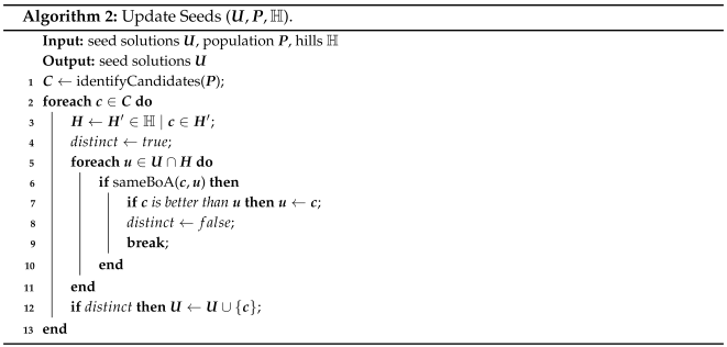
The process of updating seed solutions is shown in Algorithm 2. First, some potential seed solutions, which are termed candidate solutions $\mathit{C}$, are selected from the population. Then, for each candidate solution $\mathit{c}$, it will be checked against existing seed solutions that are located in the same hill region as $\mathit{c}$. If $\mathit{c}$ is better than an existing seed solution located in the same BoA as $\mathit{c}$, the seed solution is replaced with $\mathit{c}$. If $\mathit{c}$ does not share the same BoA with any of the seed solutions, it will be added into the set of seed solutions.

The process of updating hill regions is shown in Algorithm 3. For each hill region $\mathit{H}$, if it contains more than one seed solutions, it will be divided into multiple hill regions, whose number is equal to the number of seed solutions in $\mathit{H}$. Specifically, N random solutions are uniformly sampled in $\mathit{H}$. N is set to 100 times the number of decision variables in this paper. It is worth noting that, the evaluation of these random solutions is the only additional computational cost introduced by our method, which amounts to 100 times N times the number of evaluations for population reinitialization. These random solutions, together with the seed solutions in $\mathit{H}$, are divided into groups $\mathbb{G}$ according to the nearest-better clustering method [15]. A crucial part in the method is to set the threshold value of the nearest-better distance (NBD) for deciding whether a solution is a group center or not. However, this step is omitted in our method, as we directly select the seed solutions in $\mathit{H}$ as the group centers. The remaining part of clustering is as the same as the original method. For each group center $\mathit{u}$, any solution whose nearest-better solution is $\mathit{u}$ is assigned to the group of $\mathit{u}$. Any solution whose nearest-better solution belongs to the group of $\mathit{u}$ is also assigned to this group. After the clustering, the hill region $\mathit{H}$ is divided into multiple hill regions, each of which covers one group from $\mathbb{G}$.

$$\mathrm{B}(\mathit{x},\mathit{X})=\{{\mathit{x}}^{\prime }\in \mathit{X}|{\mathit{x}}^{\prime }\mathrm{is}\mathrm{better}\mathrm{than}\mathit{x}\},\mathit{x}\in \mathit{X}$$

(1)

$$\mathrm{NB}(\mathit{x},\mathit{X})=\underset{{\mathit{x}}^{\prime }\in \mathrm{B}(\mathit{x},\mathit{X})}{argmin}\parallel {\mathit{x}}^{\prime }-\mathit{x}\parallel ,\mathit{x}\in \mathit{X}\wedge \mathrm{B}(\mathit{x},\mathit{X})\ne \varnothing$$

(2)

$$\mathrm{NBD}(\mathit{x},\mathit{X})=\underset{{\mathit{x}}^{\prime }\in \mathrm{B}(\mathit{x},\mathit{X})}{min}\parallel {\mathit{x}}^{\prime }-\mathit{x}\parallel ,\mathit{x}\in \mathit{X}\wedge \mathrm{B}(\mathit{x},\mathit{X})\ne \varnothing$$

(3)

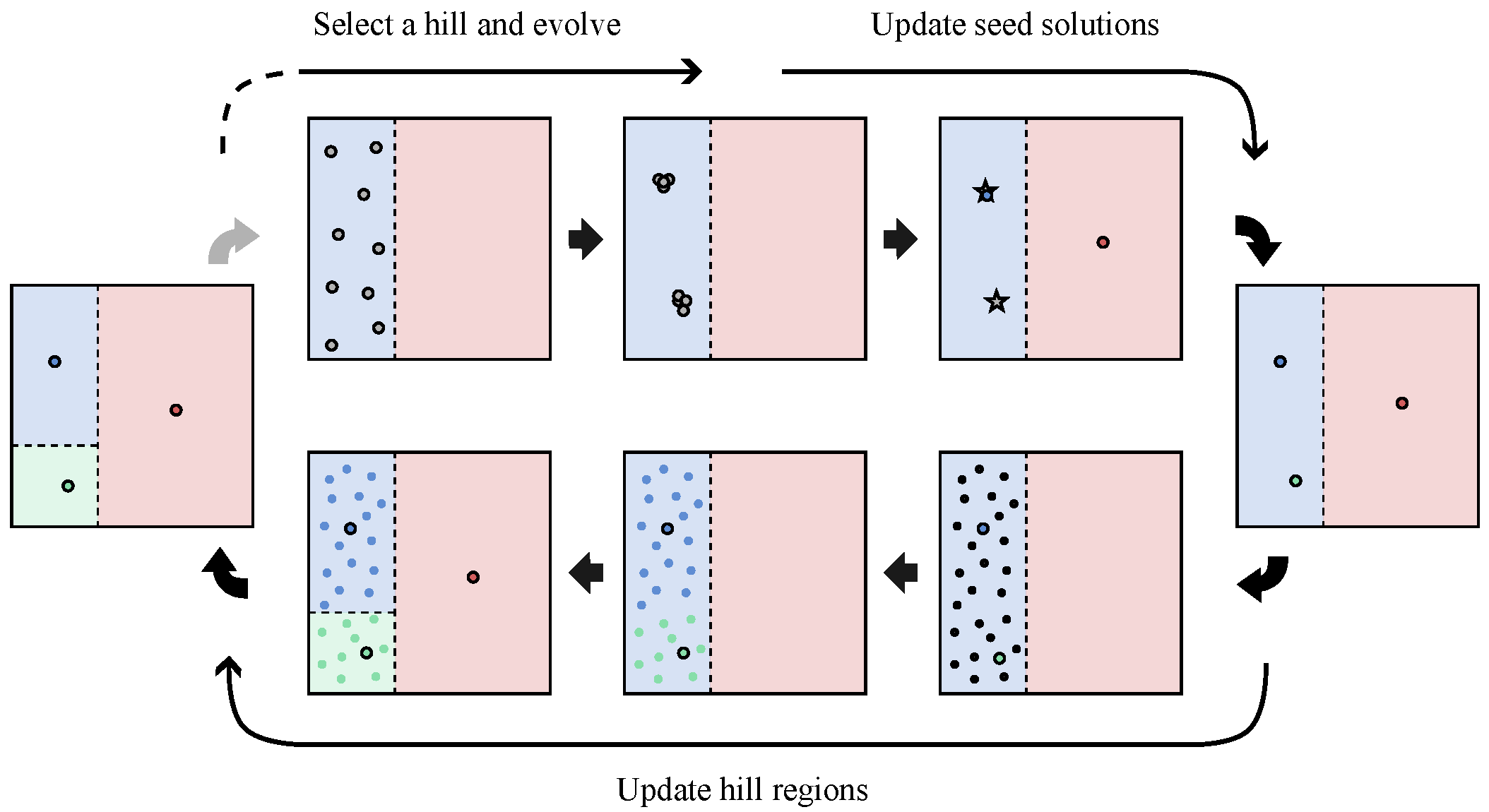
An intuitive flow of the above processes can be illustrated in Figure 2. First, a hill region is selected and the population is initialized inside the hill region. Different hill regions are denoted by rectangles of different colors. Individuals in the population are denoted by solid gray circles. Once the population is stagnant, candidate solutions, which are denoted by pentagrams, are selected from the population. Seed solutions, which are denoted by solid colorful circles, are updated according to the candidate solutions. After that, in any hill region that contains more than one seed solution, such as the blue hill region in our example, random solutions will be sampled, which are denoted by black points, and then grouped. Solutions belonging to the group of each seed solution are denoted by the points of the same color as the seed solution. After clustering, the hill region is divided into multiple hill regions, any of which contains only one group of solutions.

To meet the requirements of an ablation study, two modes have been designed for NDDCHE: the omniscient mode and the heuristic mode. The remaining details of each mode of NDDCHE including how to identify candidate solutions from the population, how to check whether two solutions are in the same BoA, and how to divide the hill region to make one hill region only contain one group of solutions, which will be provided in the corresponding subsection. The major difference between the two modes is that, in omniscient mode, the optima and BoAs are given, which make each step of NDDCHE obtain the most ideal result. So after integrating the NDDCHE in omniscient mode with a niching method, the potential improvement of NDDCHE on this niching method can be investigated thoroughly. In heuristic mode, no prior knowledge is given. So, after integrating the NDDCHE in heuristic mode with a niching method, the practical improvement of NDDCHE on this niching method can be demonstrated.

3.1. Omniscient Mode

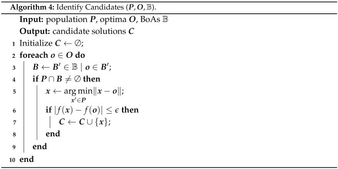
In omniscient mode, the method for identifying candidate solutions from the population is simple. As shown in Algorithm 4, since the optima and BoAs are given, individuals in each BoA can be identified, then the nearest individuals to the optimum can be found and added into the set of candidate solutions. To prevent an individual not participating in the evolution from being added to the candidates, the objective distance between the individual and the optimum is calculated. If the distance is greater than $ϵ$, which is set to ${10}^{-2}$ in this paper, the individual is discarded.

The method for checking whether two solutions are in the same BoA in omniscient mode is obvious since the BoAs are given.

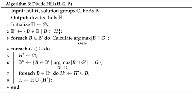
As for the method for dividing a hill region by the groups of solutions, the process is shown in Algorithm 5. The set of BoAs covered by the hill region to divide $\mathit{H}$ is denoted by ${\mathbb{B}}^{\prime }$. Each group of individuals corresponds to a new hill region. Then, for each BoA in ${\mathbb{B}}^{\prime }$, it is assigned to the new hill region whose corresponding group of individuals occupies the most in this BoA.

3.2. Heuristic Mode

In heuristic mode, the specific method for identifying candidate solutions depends on some details of the niching method integrated with NDDCHE as follows:

• For niching methods with seed solutions or analogous structures, the archive solutions are directly selected as the candidate solutions;
• For niching methods without seed solutions or analogous structures,

  –

  If a clustering method is adopted in the niching method, the group centers are selected as the candidate solutions;

  –

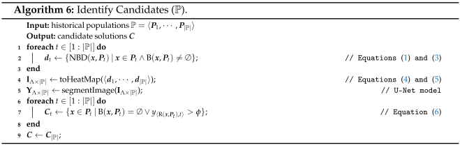
  Otherwise, a novel method based on image segmentation model is adopted to select the candidate solutions as the process shown in Figure 3 and Algorithm 6.

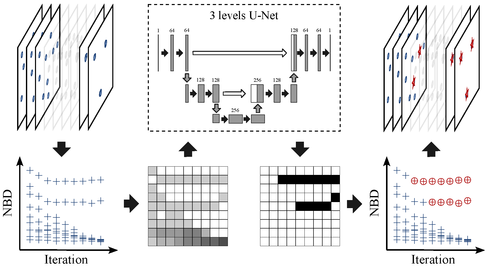
The idea behind the method based on the image segmentation model is that, after calculating the distribution of NBDs of individuals in the population according to Equations (1) and (3), the variation of the distribution exhibits a clear pattern with the evolution. As the example shown in Figure 3, the left upper graph shows the variation of distribution of individuals in the 2D search space with the evolution, and the left lower graph shows the corresponding variation in NBDs. For most individuals, their NBDs decreased rapidly with the growth of iteration, except for the three individuals. Two of them have their NBDs shown in the graph. The remaining individual is the best individual who does not have a nearest-better solution. For these three individuals whose NBDs are outliers, they are also the three centers that the population is converging towards.

To automatically identify these outliers, the variation in the distribution of NBDs is transformed into an image ${\mathbf{I}}_{\Lambda \times \left|\mathbb{P}\right|}$ according to Equations (4) and (5). $\Lambda$ denotes the specified resolution of NBD, which is set to 50 in this paper, and $i_{\langle r,t\rangle }$ denotes the value of pixel in the r-th row and t-th column. Input the image through a 3-level U-Net model [26], an output image ${\mathbf{Y}}_{\Lambda \times \left|\mathbb{P}\right|}$ highlighting the pixels corresponding to the outliers is generated, where $y_{\langle r,t\rangle }$ denotes the value of pixel in the r-th row and t-th column. According to the image, the candidate solutions in each generation can be obtained, where the threshold value $\varphi$ is set to $0.5$. For the ease of use, the candidate solutions in the last generation is selected. To prevent the loss of potential seed solutions during the evolution, candidate solutions from other generations can also be selected.

$$\begin{array}{c}\hfill i_{\langle r,t\rangle }={\displaystyle \frac{2}{\pi }}arctan\left(\right|\{d\in {\mathit{d}}_t|{\displaystyle \frac{r-1}{\Lambda }}\le {\displaystyle \frac{d}{d_{max}}}<{\displaystyle \frac{r}{\Lambda }}\}\left|\right),\\ \hfill r\in [1:\Lambda ],t\in [1:|\mathbb{P}\left|\right]\end{array}$$

(4)

$$d_{max}=max\left(\right\{max\left({\mathit{d}}_t\right)|t\in [1:\left|\mathbb{P}\right|\left]\right\})$$

(5)

$$\mathrm{R}(\mathit{x},{\mathit{P}}_t)=\lceil \Lambda ·{\displaystyle \frac{\mathrm{NBD}(\mathit{x},{\mathit{P}}_t)}{d_{max}}}\rceil ,\mathit{x}\in {\mathit{P}}_t\wedge \mathrm{B}(\mathit{x},{\mathit{P}}_t)\ne \varnothing$$

(6)

The method for checking whether two solutions are in the same BoA in heuristic mode is through the hill–valley function [22], where the number of samples between the two solutions is set to 2.

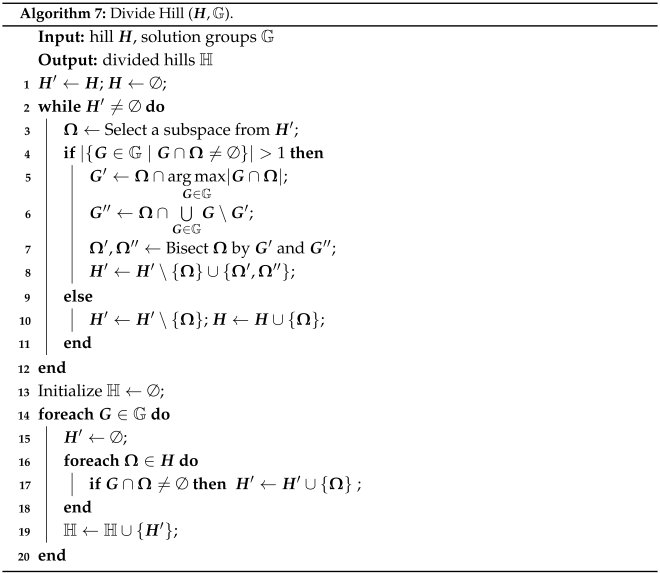
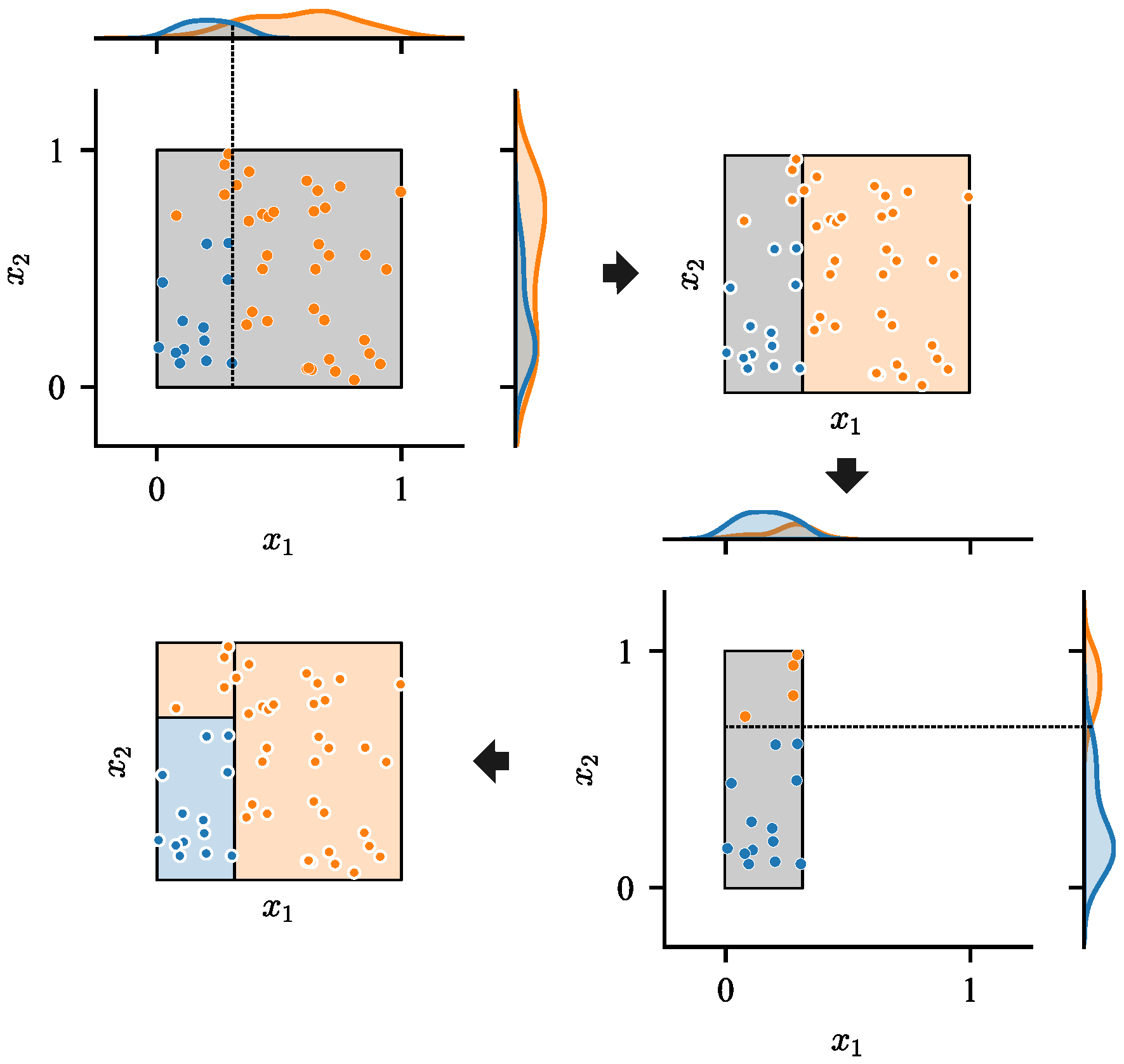
The method for dividing a hill region by the groups of solutions in heuristic mode is shown in Algorithm 7. It consists of two parts. In the first part, the subspaces composing the hill region are continuously bisected until each of the subspaces only contains individuals from the same group. For continuous search spaces, which are concerned by this paper, a subspace is bisected along the axes. Regarding the specific dimension to be selected and the specific position to split in this dimension, an intuitive illustration is shown in Figure 4.

First, in each dimension, the kernel density estimations for the largest solution group ${\mathit{G}}^{\prime }$ and other solutions ${\mathit{G}}^{″}$ are calculated separately, whose probability density functions are represented by areas of corresponding colors. After that, the dimension where two functions have the minimum intersection is selected. The intersection of two probability density functions $f_1\left(x\right)$ and $f_2\left(x\right)$ is ${\int }_{-\infty }^{\infty }min(f_1\left(x\right),f_2\left(x\right))dx$, which is approximately calculated by $|{\mathit{G}}^{\prime }\cup {\mathit{G}}^{″}|$ uniform samples between the minimum and maximum values of solutions of ${\mathit{G}}^{\prime }\cup {\mathit{G}}^{″}$ in this dimension.

Finally, the first equiprobability point of the two functions in this dimension is determined as the position to split, which is also approximately located by the uniform samples.

In the second part, the subspaces are divided into groups, each of which composes a new hill region. Subspaces in which individuals are from the same group are assigned to the same hill region.

4. Experiments

With the hierarchical divide-and-conquer framework for niching methods implemented as NDDCHEs in both omniscient mode and heuristic mode, a set of targeted experiments can be conducted in phased stages.

The experiments in the first stage, which are shown in Section 4.1, are designed for answering why the hierarchical divide-and-conquer framework is essentially different from existing niching techniques, which have been theoretically analyzed in Section 2. This is achieved by investigating the effect of NDDCHE in omniscient mode, where the optima and BoAs of the problem are given, and thus the ideal effect of NDDCHE on niching methods can be demonstrated. For this purpose, the free peaks [27] model is adopted to generate test problems, where the boundaries of BoAs can be clearly defined, and exponential differences in the sizes of the BoAs $v_1,\cdots ,v_k$ can be specified as in Equation (7),

$$\forall i\in [2:k],{\displaystyle \frac{v_i}{{\sum }_{j=1}^{i-1}{v}_j}}=2,$$

(7)

where k denotes the number of optima. The contour lines of fitness of an instance problem with $k=7$ in two-dimensional search space are shown in Figure 5, where the locations of the optima are denoted by white crosses.

The experiments in the second stage, which are shown in Section 4.2, are designed for answering how feasible the hierarchical divide-and-conquer framework is. This is achieved by investigating how much difference would be made if the methods in omniscient mode are replaced with corresponding methods in a heuristic mode. An ablation study on the effectiveness of each of the two parts of NDDCHE is also conducted through this process. The first part consists of methods for updating seed solutions, while the second part consists of methods for updating hill regions. These experiments will show how closely the heuristic mode approximates the performance of the omniscient mode.

The experiments in the third stage, which are shown in Section 4.3, are designed for showing the effect of NDDCHE in complex cases, including when the number of decision variables is much higher than 2, the distribution of optima is chaotic, and the fitness landscape in each BoA is ill-conditioned and asymmetric.

4.1. Effect of NDDCHE in Omniscient Mode

To prove the generalization ability of the framework, NDDCHE is integrated with representative niching methods with each category of niching technique. The selected niching methods are as follows.

• For the radial repulsion technique, two state-of-the-art niching methods with this technique, which are RS-CMSA [6] and PMODE [7], are selected.
• For the nearest neighbors technique, in most state-of-the-art niching methods with this technique, it is combined with other techniques. So k-nearest PSO (kNPSO) [1], which is a recently proposed PSO that only uses the nearest neighbors technique to achieve a great performance, is selected.
• For the specified number of groups technique, NSDE [12] is selected as it is a representative niching method that achieves niching only through the specified number of groups technique.
• For the adaptive number of groups technique, NEA2 [15], which is a representative niching method with this technique and still competitive, is selected.
• For the valley detection technique, a state-of-the-art niching method with this technique, namely HillVallEA [25], is selected.

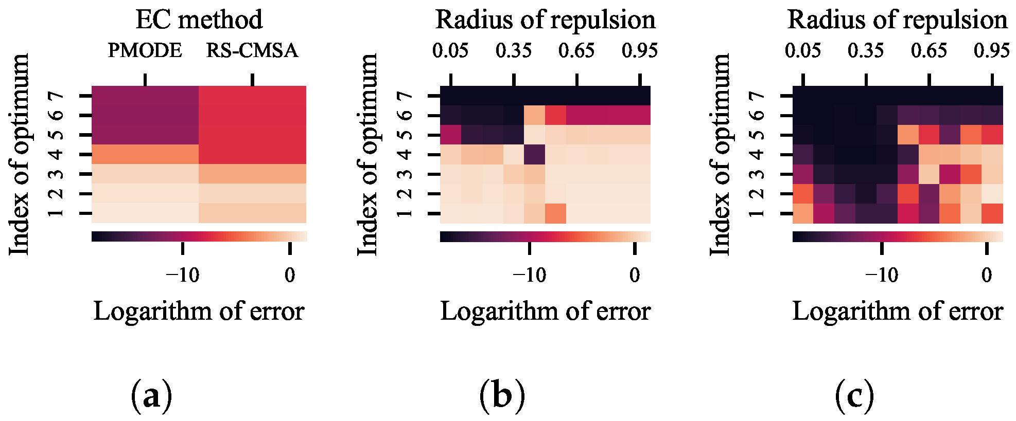
Firstly, 100 independent runs of RS-CMSA and PMODE on the test function are conducted. The random seeds for the 100 runs are set to 1/101,…, 100/101, respectively. The maximum number of evaluations is set to 50,000. The population size in PMODE is set to 20. The average error for each optimum is shown in Figure 6a. The error to an optimum is defined as the objective distance between the optimum and the best solution found within its BoA. The clear boundaries of the BoAs facilitate an accurate differentiation of the errors to different optima.

In this heat map, each column corresponds to a niching method. The color of grid in a specific column denotes the average value of the logarithmic error to the corresponding optimum. According to Equation (7), the smaller the index of an optimum, the smaller the size of its BoA. So the results clearly indicate that, for both RS-CMSA and PMODE, the smaller the size of a BoA, the lower the probability of locating the optimum in it.

As mentioned in the related works, setting the threshold distance for radial repulsion between a more appropriate range can improve the performance. However, the threshold distance is adaptively adjusted in both RS-CMSA and PMODE, which affords no opportunity for us to attempt. To this end, a recently proposed DE with the radial repulsion technique, namely local repulsion DE (LRDE) [1], is adopted. In LRDE, by setting the radius of repulsion to a value in the range of [0:1], the threshold distance for radial repulsion becomes the product of the radius of repulsion and $V^{1/D}$, where V and D denote the volume and dimension of the search space, respectively.

After 100 independent runs of LRDE with the radius of repulsion set to different values, where the maximum number of evaluations is set to 50,000 and the population size is set to 20, the error for each optimum is shown in Figure 6b. Each column shows the result of LRDE with a specific value of the radius of repulsion. The results prove that, by setting the threshold distance for radial repulsion within a more suitable range, which is around $0.35·V^{1/D}$ in the experiment, a better performance can be achieved. However, although setting the radius of repulsion to $0.35$ makes LRDE competitive with the two state-of-the-art niching methods, it is still hard to further improve it by finding a more suitable value of the radius of repulsion, especially in practical cases.

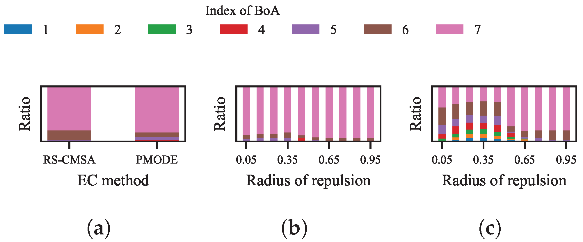
At this juncture, it is imperative to revisit the perspectives summarized in Section 2. We believe that existing niching techniques share a common limitation: while it is possible to increase the probability of finding less-attractive optima by tuning parameters, it is difficult to address the imbalance of search resources among the optima caused by the disparity in their attractiveness. To prove this point, the evaluations spent in the BoA of each optimum in the previous experiments are demonstrated in Figure 7a,b. According to the results, for either RS-CMSA, PMODE, or LRDE with various radii of repulsion, all spent the red majority of evaluations within the largest BoA.

As the proposed framework claims to balance the evaluations between different optima, 100 independent runs of LRDE integrated with NDDCHE in omniscient mode and with the radius of repulsion set to different values are conducted. The maximum number of evaluations is set to 50,000 and the population size is set to 20. The results are shown in Figure 6c and Figure 7c.

According to the results, the numbers of evaluations spent in different BoAs are significantly balanced by NDDCHE in omniscient mode. We can also observe that the corresponding performance of LRDE is significantly improved. For LRDE with each value of radius of repulsion, there has been a notable reduction in its errors for optima in smaller BoAs, which indicate the growth of probabilities of finding these optima. With the radius of repulsion set to the most suitable value observed in the previous experiment, i.e., $0.35$, all seven optima can be found while the maximum of evaluations is still 50,000.

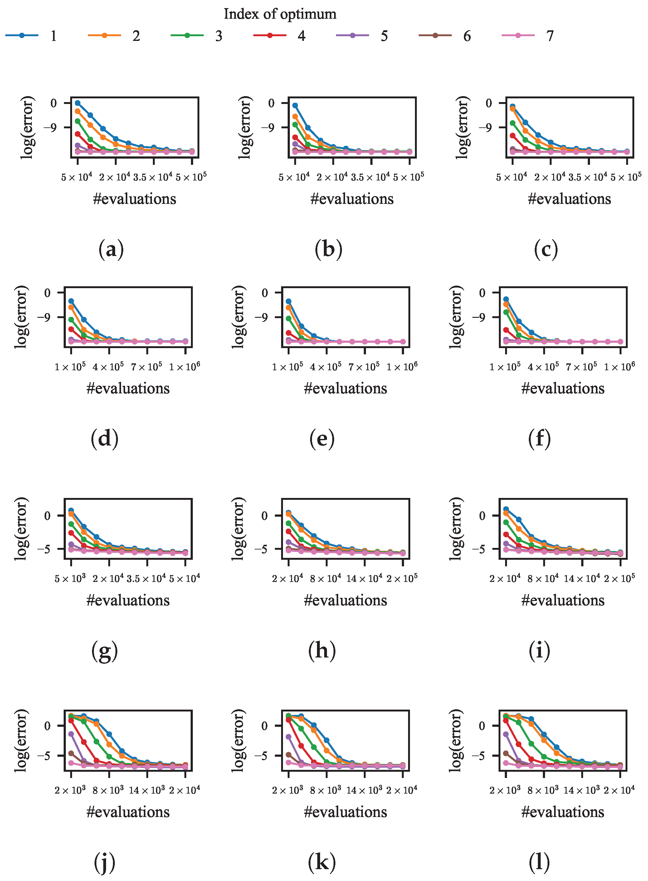
As for the niching methods with the four remaining categories of niching techniques, the effect of tuning their common key parameters, i.e., the size of the population, is observed first. The observation is through a restart strategy in which, upon detecting stagnation in the population, it is reinitialized and its size is doubled. Another restart strategy in which the size of the population remains unchanged in each restart is used as the background for comparison. In the four selected niching methods, HillVallEA and NEA2 have their own criterion for judging the stagnant population. For kNPSO and NSDE, if none of the individuals have improved in the last 10 generations, the population is considered stagnant.

After 100 independent runs of the four niching methods with different restart strategies on the test function, the variation of the average error for each optimum is shown in Figure 8a–h. The initial size of the population in kNPSO, NSDE, and NEA2 is set to 20. Each line of a color denotes the variation of the average error to a specific optimum.

According to the results, for all four niching methods, the error for each optimum decreases with the evolution when the size of the population is constant or doubled upon each restart. This indicates that both restart strategies contribute to finding more optima. Additionally, the speed of decreasing is higher when the size of the population is doubled at each restart, which indicates that a larger size of population increases the probability of these niching methods finding the optima in smaller BoAs.

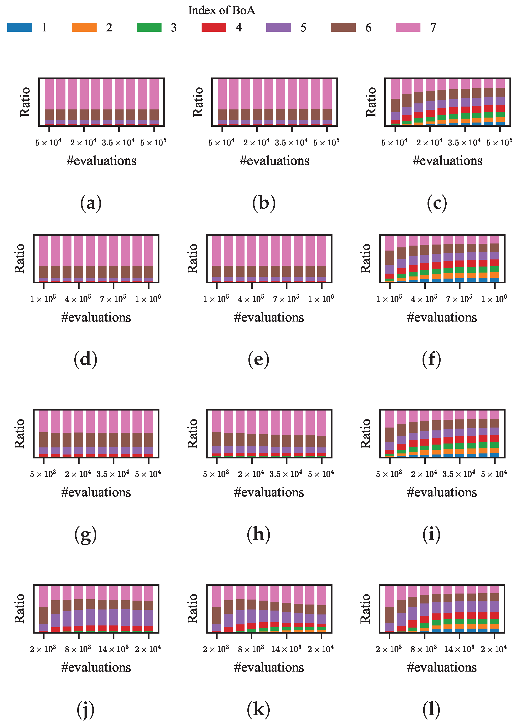
Nonetheless, the limitations previously discussed regarding LRDE are also evident in the four methods currently under examination. This can be observed from the corresponding variation of the ratio of evaluations spent by these methods in each BoA during the evolution, which is shown in Figure 9a–h. For kNPSO, NSDE, and NEA2, the significant imbalance between evaluations in each BoA almost remain unchanged during the evolution regardless of whether the population size doubled or not at each restart. As for HillVallEA, although the imbalance decreases a bit at the early stage of evolution, it soon keeps unchanged or even increase at the later stage.

To demonstrate the effect of NDDCHE on addressing their limitations, 100 independent runs of the four niching methods integrated with NDDCHE in omniscient mode on the test function are conducted. The results are shown in Figure 8i–l and Figure 9i–l. These results show that, when NDDCHE is integrated with any of the four niching methods, the imbalance between evaluations in different BoAs continuously decreases until the ratios of evolutions in each BoA are almost equal. The results also show a significant difference in the speed of error decreasing between the niching methods with and without NDDCHE.

The above experimental results imply that only through changing the area for initialization from the entire search space to a randomly selected hill region that learned from evaluated solutions can the distribution of searches for different optima be balanced, and thus can the probability of locating optima of lower attractiveness be enhanced.

4.2. Effect of NDDCHE in Heuristic Mode

The above experiment shows the ideal effect of the proposed hierarchical divide-and-conquer framework. However, although the hill regions are gradually learned from scratch in NDDCHE in omniscient mode, the locations of the optima and the boundaries of BoAs are utilized to ensure the accuracy of learning, which is far beyond the practical cases. So, in the following experiments, the parts of NDDCHE in omniscient mode are replaced with their heuristic versions to demonstrate the feasibility of the proposed framework.

An ablation study on the effect of each of the two major parts of NDDCHE is also conducted during this process. Firstly, the methods for updating seed solutions in omniscient mode are replaced with their heuristic versions, while that for updating hill regions remain the omniscient versions. The framework in this mode is named NDDCHE in the half-heuristic mode for ease of description. A comparison between NDDCHE in omniscient mode and that in half-heuristic mode can show the effect of updating seed solutions in practical cases. Next, a comparison between NDDCHE in half-heuristic mode and that in heuristic mode, where all methods in NDDCHE are in their heuristic forms, can show the effect of updating hill regions.

For LRDE, 100 independent runs of LRDE with NDDCHE in half-heuristic mode and LRDE with NDDCHE in heuristic mode are conducted on the test problem. The results are shown in Figure 10b,c. For ease of comparison, the result of LRDE with NDDCHE in omniscient mode is shown in Figure 10a. It can be observed that the errors of LRDE integrated with NDDCHE in half-heuristic mode are a bit larger than those in omniscient mode, and there is no significant difference between the effects of NDDCHE in half-heuristic mode and NDDCHE in heuristic mode.

As for the four remaining niching methods, 100 independent runs with NDDCHE in half-heuristic mode and them with NDDCHE in heuristic mode are conducted on the test problem. The results are shown in Figure 11e–l. Like LRDE, the result of the four remaining niching methods with NDDCHE in omniscient mode is shown in Figure 11a–d for ease of comparison. The results demonstrate that the decrease in the error in heuristic mode is a bit slower than that in half-heuristic mode, which is also a bit slower than that in omniscient mode. However, compared with the difference between whether the EC method uses NDDCHE or not, the difference between niching methods using different modes of NDDCHE is almost negligible.

Above all, the methods in heuristic mode or half-heuristic mode basically achieve the same effect as the methods in omniscient mode on the test problem, which indicates that the effectiveness of NDDCHE can be guaranteed without prior knowledge about optima or BoAs.

4.3. Effect of NDDCHE in Complex Cases

Although there exists an exponential difference in the size of the BoA between the optima in the problem used in the above experiments, some other factors may also increase the difficulty of the problem. As shown in Figure 5, the distribution of the optima shows a fractal structure in the previous test problem, which is chaotic in many cases. Additionally, the fitness landscape in the BoA of each optimum is symmetric and isotropic around the optimum in the test problem, which might be asymmetric and ill-conditioned in practical cases.

To investigate the effect of NDDCHE in those complex cases, we use the free peaks [27] to generate eight test problems F1 to F8. Their fitness landscapes are shown in Figure 12. In these problems, the distribution of optima is randomly determined, and some random transformations are used to make the fitness landscape in each BoA ill-conditioned and asymmetric. The exponential difference in size of the BoA between optima is kept, which ensures that there is a significant difference in attractiveness between optima.

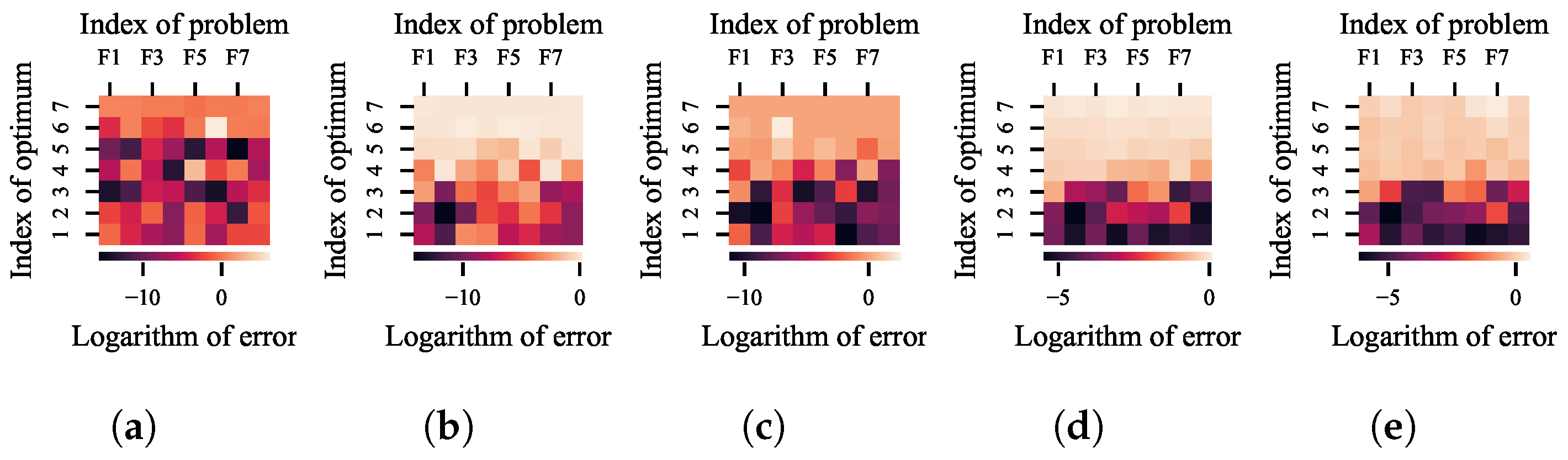
For each of the five selected niching methods, after 100 independent runs on the above eight test problems, the average improvement in error for each optimum made by NDDCHE is shown in Figure 13. The improvement in error is calculated as the logarithmic error of a niching method integrated with NDDCHE minus the logarithmic error of the method without NDDCHE. Each heat map corresponds to a specified niching method. In the heat map, each column refers to the improvement in error on a specified problem, and each row refers to the difference in error to a specified optimum. The population size of LRDE, kNPSO, NSDE, NEA2 is set to 20. The number of maximum evaluations of LRDE, kNPSO, NSDE, NEA2, and HillVallEA is set to 1 × 10⁵, 2 × 10⁶, 4 × 10⁶, 1 × 10⁵, and 1 × 10⁵, respectively. The radius of repulsion of LRDE is set to 0.35.

According to the results, as a lower logarithm of error indicates a smaller error, NDDCHE significantly decreases the errors for optima in most cases. In general, the heat maps of the latter four methods exhibit a distinct pattern: errors for optima with smaller indices have lesser decrements. This is because optima with smaller indices possess larger BoAs, making them more attractive and thus easier to locate even without using NDDCHE. Conversely, for optima with larger indices and consequently smaller BoAs, the application of NDDCHE leads to substantial decrements in the average error to these optima, indicating a significant enhancement in the probability of locating them.

Additionally, The results also demonstrate that the improvement achieved by NDDCHE depends on the niching method integrated with it. There is a clear similarity between the heat maps for kNPSO and NSDE, which indicate the similarities between their operators for local search and their niching techniques. The heat maps for NEA2 and HillVallEA also exhibit remarkably similar patterns, which is primarily due to the similarity between their core algorithms. As for LRDE, its niching technique is markedly distinct from the niching techniques employed by the other four niching methods. This distinction is so pronounced that the heat map of LRDE bears little to no resemblance to those of the latter methods.

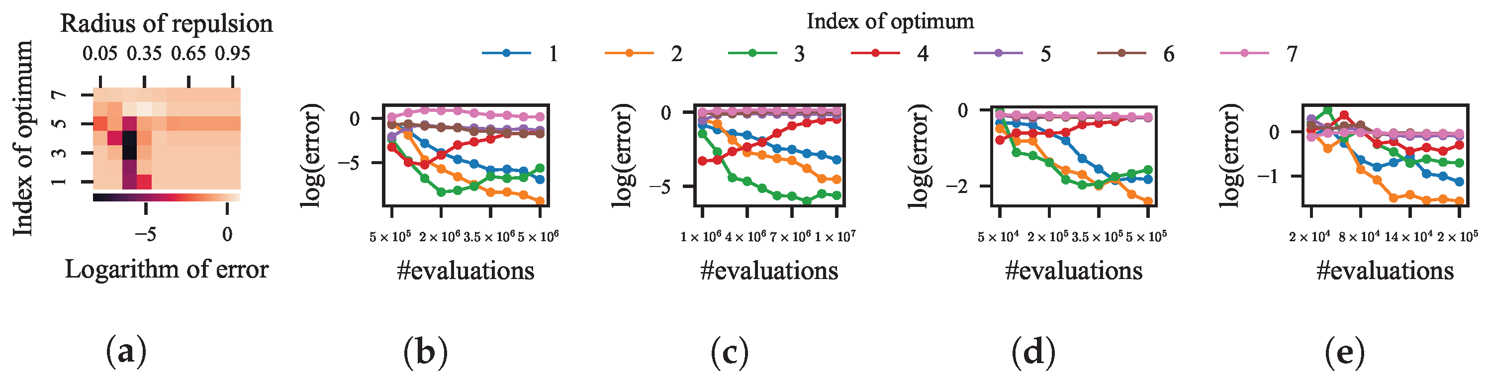
In addition to irregular fitness landscapes, the increase in the dimensionality of the problem’s decision space also escalates the search difficulty. To investigate the effect of NDDCHE when the number of decision variables is much higher than two, 100 independent runs of the five selected niching methods on a 10-D test problem are conducted. As was the case in previously tested problems, there also exists an exponential difference in the size of BoA between the seven optima of the 10-D test problem as described in Equation (7).

The maximum numbers of evaluations for LRDE, kNPSO, NSDE, NEA2, and HillVallEA are set to $5\times {10}^6$, $5\times {10}^6$, $1\times {10}^7$, $5\times {10}^5$, and $2\times {10}^5$, respectively. The population size for LRDE, NSDE, or NEA2 is set to 20. As for kNPSO, the speed of convergence decreases drastically with the growth of the number of decision variables when its number of neighbors k remains to be 2, so k is set to 5 and the population size is set to 100. The results are shown in Figure 14, where (a) demonstrates the heat map of the average improvement in error for each optimum made by NDDCHE on LRDE with different radii of repulsion, and (b–e) show the variation in the average improvement in error for each optimum made by NDDCHE on the remaining four EC methods.

According to the results, NDDCHE decreased the errors for optima with smaller BoAs for LRDE in most cases, especially when the radius of repulsion was set to 0.35. As for the remaining four EC methods, the incorporation of NDDCHE resulted in at least one order of magnitude enhancement in the rate of reduction in errors for optima with smaller BoAs.

Above all, the above experimental results demonstrate the effectiveness of NDDCHE in complex cases, i.e., when the problem has a higher number of decision variables or an irregular fitness landscape in each BoA, a hierarchical divide-and-conquer framework can still enhance the abilities of niching methods in locating optima with lower attractiveness.

5. Conclusions

This paper reviews and analyzes representative niching techniques used in existing methods. Although both of them can enhance their abilities in terms of locating less-attractive optima by tuning their key parameters, it is hard for them to balance search resources over optima with significant differences in attractiveness, which limits their potentials as the difference further increases.

To address the above issue, this paper proposed a hierarchical divide-and-conquer framework for niching methods, which is named NDDCHE. From the search result of a niching method, the framework identifies seed solutions, any two of which do not share the same BoA, and gradually divide the search space into smaller hill regions, each of which corresponds to the estimation of the BoA of an optimum that has already been detected. After that, the niching method is reinitialized in one of the hill regions, which contributes to detecting more seed solutions.

The framework is integrated with five representative niching methods with different categories of niching techniques. The experiments on test problems with exponential differences in the size of BoA between the optima proved that NDDCHE enables each niching method to achieve a much more balanced distribution of search resources among the optima and thereby improves the ability to find optima with less attractiveness without tuning any parameters.

Moreover, although NDDCHE was compared with parameter tuning in some experiments, it does not conflict with the latter. Specifically, if desired solutions cannot be found by a niching method, NDDCHE can be initially employed to fully exploit the potential of the niching method under the current parameter settings. When no additional seed solutions can be identified within any hill region, the parameter should then be tuned. If a new seed solution is found after tuning the parameter, NDDCHE can then continue to fulfill its role.

It is worth noting that, in the current framework, no priority is assigned to different hill regions, as the population is re-initialized in a randomly selected hill region. Clearly, the number of BoAs requiring further subdivision varies across different hill regions, and the fitness values of different local optima also differ. Therefore, if hill regions containing more BoAs or better local optima could be prioritized in the search, the search efficiency could be further improved. Predicting the differences in search potential among various hill regions will be the focus of our next steps.