Objective Function Formulation to Optimize Control Structure Parameters Using Nature-Inspired Optimization Algorithms

Abstract

This paper uses a nature-inspired optimization algorithm to discuss the automatic selection of control structure parameters. The commonly used quality indicators are presented and analyzed for the optimization process of the control system. Moreover, the possibilities of formulating objective functions for nature-inspired optimization algorithms that can be successfully used to solve multi-objective constrained optimization problems are presented. The proposed general methodology was presented and discussed in detail using an example, which is published in the open-source repository Mathwork FileExchange. Theoretical aspects are validated in the case studies for automatic tuning of the hysteresis and PI controller.

1. Introduction

Automatic control is the most basic task used in the industry. To obtain a satisfactory system response, many control structures have been developed. Because complex control systems are not trivial to analyze, selecting the control structure parameters does not seem trivial. Therefore, automatic tuning procedures based on nature-inspired optimization algorithms have attracted significant attention in recent years. Such auto-tuning allows the user to obtain optimal system responses, in terms of a defined objective function, regardless of the control system complexity. The proper formulation of the objective function is crucial for the proper optimization process. In general, higher values of control structure proportional gains allow for the achievement of better dynamics. On the other hand, the limitation of the physical system’s accuracy is related to delays, quantization, measurement noises, or unmodeled non-linearities during control structure design, which limits the possible dynamic of the control system. The objective function requires expert knowledge of the control system to maximize the system’s dynamics and still provide a chattering-free control signal. However, formulating the objective function seems less difficult than selecting the optimal control structure parameters. It should be noted that automatic selection of control structure parameters was intensively researched in recent years. The following control structures were considered: Proportional–integral–derivative (PID) controllers [1,2,3,4,5,6], two degree-of-freedom PID (2DoF PID) [7], state-feedback controllers [8,9,10,11], multi-resonance controllers [12], neural network-based controllers [13], fuzzy logic controllers [14], and event-triggered controllers [15]. Moreover, selecting nature-inspired optimization algorithms is not crucial for properly operating automatic tuning. Due to the no free lunch theorem, there is no best algorithm to solve all optimization problems. In the case of global optimization algorithms, which are nature-inspired, every algorithm can solve the same problem. The difference is related to the optimization time required to find the global optimum. Therefore, the selection of the optimization algorithm can be interpreted as user preferences. The most commonly used in the literature for automatic tuning are particle swarm optimization [2,16,17], artificial bee colony algorithm [10,12], and grey wolf optimizer [13,18,19].

The simple objective function with the integral time absolute error (ITAE) indicator was used in [17,20], while the particle swarm optimization and Jaya optimization algorithms were used to solve the problem, respectively. Robust two-degree-of-freedom state-feedback PI-controller tuned by the particle swarm optimization algorithm for an automatic voltage regulation system was proposed in [21]. The objective function was not presented, except to mention that it utilizes the output and control signal. In [22], a nature-inspired optimization algorithm has been employed to obtain the weighting matrices values needed to calculate discrete state-feedback speed controllers for permanent magnet synchronous motor drive. This approach selects eight controller parameters using one weighting factor in the objective function. The objective function was based on minimizing the speed and current error in the d-axis of the rotational coordinate system. The penalty function was related to changes in the control signal, and this part has an additional coefficient that the user should select. In [23], the particle swarm optimization algorithm is used to optimize the linear quadratic regulator for a voltage source inverter with an LC output filter. The proposed objective function is based on the ISE indicator and the penalty for control signal chattering. The 15-D problem has been reduced to the selection of a single penalty coefficient. The design process of the adaptive neural controller implemented for a non-linear object using grey wolf optimizer was presented in [19]. The objective function was based on the integral-squared time-squared error (ISTSE) indicator extended by additional penalties for error and control signal changes to limit excessive growth of the optimized values. Such an objective function required the determination of two coefficients using the trial-and-error approach. In [8], the optimal parameters of the state-feedback controller were selected using an artificial bee colony algorithm with a non-trivial objective function. To minimize steady-state oscillations in permanent magnet synchronous motor drive, an additional component related to steady-state oscillations was added. Unfortunately, an additional weighting factor was required to balance the oscillation damping and good step response indicators. The proportional–integral–derivative (PID) controller was automatically tuned in [24]. The objective function was created by determining the required overshoot, minimizing the settling time and steady-state error. In [25], hybrid simulated annealing and manta ray foraging optimization algorithms were used to find the optimal PID controller parameters. The objective function does not utilize standard indicators such as integral absolute error (IAE) or integral-squared error (ISE). It is based on the value of rising time, overshoot, and steady-state error. In [12], the auto-tuning of a multi-resonant current controller is proposed with a nature-inspired optimization algorithm. The objective function was free of additional weighting factors and used the ISE indicator. However, additional requirements, such as a noise-free control signal and a minimal rise time, were determined. The violation function was used to ensure that the chattering would not appear. The second requirement ensured that the rise time would not be less than the predefined value. In such a case, the proposed objective and violation functions do not require additional weighting factors. To solve the constrained optimization problem, Deb’s rule has been utilized [22].

To summarize the previously mentioned and discussed papers, nature-inspired optimization algorithms can be successfully applied to determine control structure parameters. The selection of the optimization algorithm is less important compared to the proper formulation of the objective function. The objective function must be determined for a particular case. In this paper, the methodology of formulating objective functions is presented and proposed in the form of the algorithm supported by an example. The authors discuss different indicators, the formulation of the objective function and the violation function, constraint-handling techniques, and the weighting factor selection process. The novelty of this paper is related to the proposed algorithm describing, step by step, how to apply nature-inspired optimization algorithms to select the optimal control structure parameters. To the best of the authors’ knowledge, such an algorithm has not been presented in the literature before. This paper is summarized with case studies in which the objective function is determined and the simulation results are presented.

This paper is organized as follows. Section 2 introduces the review of the system response performance indicators: the basic integral performance indicators, the step response indicators, and, finally, the examples of the formulation of additional requirements. The general idea of the application of nature-inspired optimization algorithms for multi-objective constrained optimization problems is presented in Section 3. The proposed methodology for selecting structure parameters using nature-inspired optimization algorithms is described in Section 4. In addition, the in-depth analysis of a simple example is included to provide better readability and understanding of the proposed methodology. Section 5 presents two real-world examples, where the proposed methodology can be applied. Section 6 concludes this study.

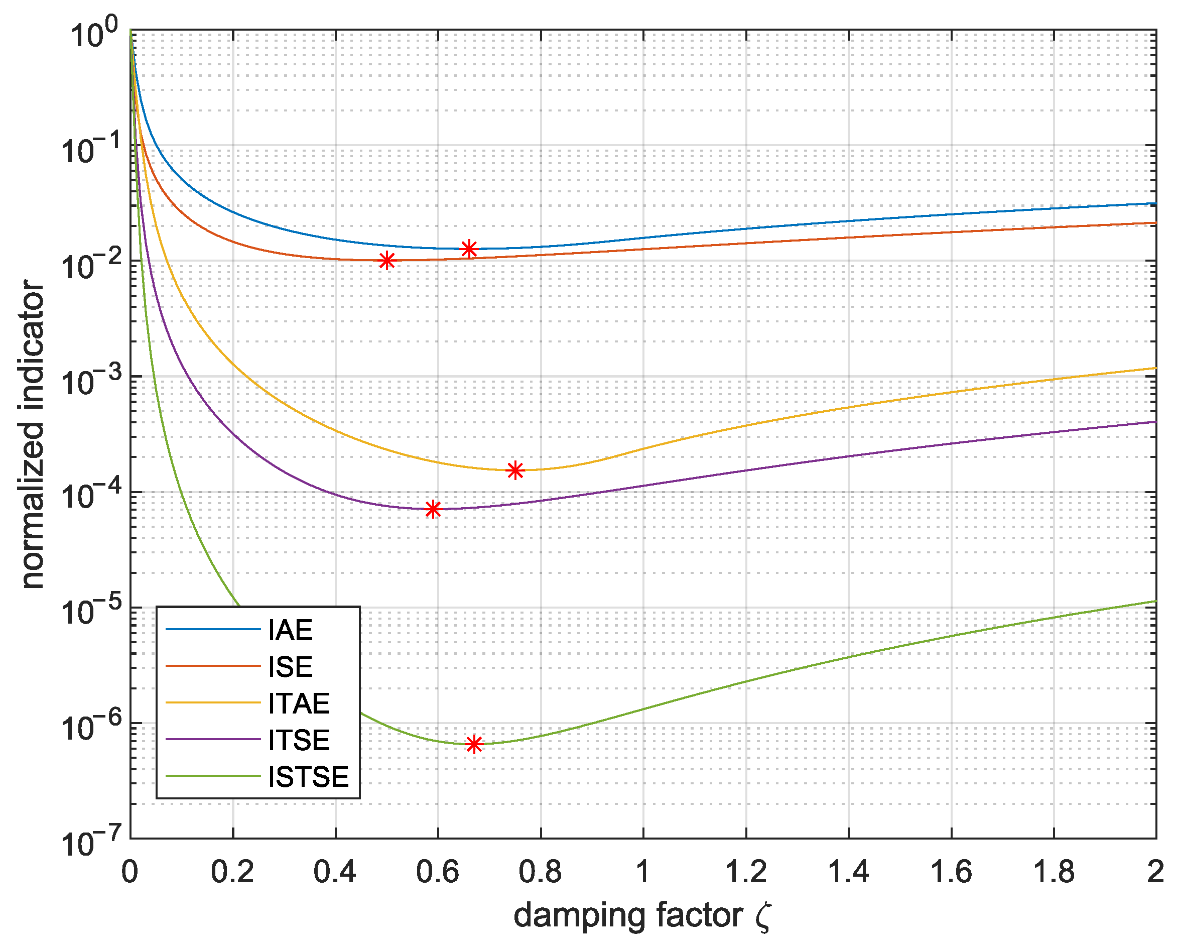
2. Performance Indicators of System Response

The optimization problem is based on the numerically defined objective function. In control theory, the basic indicators of system response quality are related to the integral of the control loop error. Additional criteria can be easily defined for evaluating the response of the system based on the step input signal, i.e., rise time, settle time, and percentage overshoot. In this section, these criteria are formulated and described in terms of how they can be used in the formulation of objectives.

2.1. Basic Criteria

Indicators are based on the integration in time from 0 to T on some function of the control loop error (e), i.e., the squared or absolute error. The list of the basic criteria that are commonly used in automatic tuning of the parameters is as follows:

• Integral-Squared Error (ISE):

  $$\mathrm{ISE}={\int }_0^T{e}^2\left(t\right)dt$$

  (1)
• Integral Absolute Error (IAE):

  $$\mathrm{IAE}={\int }_0^T\left|e\left(t\right)\right|dt$$

  (2)
• Integral Time Squared Error (ITSE):

  $$\mathrm{ITSE}={\int }_0^{T}t·e^2\left(t\right)dt$$

  (3)
• Integral Time Absolute Error (ITAE):

  $$\mathrm{ITAE}={\int }_0^{T}t·\left|e\left(t\right)\right|dt$$

  (4)
• Integral-Squared Time-Squared Error (ISTSE):

  $$\mathrm{ISTSE}={\int }_0^T{t}^2·e^2\left(t\right)dt$$

  (5)

To present the impact of the selection of the above criteria, the second-order system is considered:

$$G_{II}\left(s\right)={\displaystyle \frac{k{\omega }_n^2}{s^2+2\zeta {\omega }_{n}s+{\omega }_n^2}}$$

(6)

where k is static gain, $\zeta$ is the damping factor, and ${\omega }_n$ is the natural frequency. In Figure 1, all of the above-mentioned indicators are presented in the damping factor domain for the following parameters: $k=1$ and ${\omega }_n=1$.

The red markers are used to mark the minimal values of the plots because automatic tuning using a nature-inspired optimization algorithm minimizes one of these indicators. Comparing the additional time in the integral (ISE, ITSE, and ISTSE), it can be seen that the damping factor moves towards a higher damping factor. It should be noted that a higher power of time allows us to reduce the oscillations and settling time because of the higher importance of higher time values. Furthermore, it should be noted that the minimal values differ significantly. In such a case, the weighting factor in objective functions must be selected to the used integral indicator due to different orders of magnitude.

2.2. Step Response Indicators

The shape of the system response cannot be simply determined based on the value of basic indicators, e.g., ISE. In addition, such quality indicators are highly dependent on measurement noises (in the case of online automatic tuning). For this reason, the step indicators (SIs) are commonly used to determine the required response of the system. The commonly used step indicators are as follows:

• Percentage Overshot (PO):

  $${\mathrm{SI}}_{\mathrm{PO}}={\displaystyle \frac{maxy\left(t\right)-y(\infty )}{y(\infty )-y\left(0\right)}}$$

  (7)
• Rising Time (RT):

  $${\mathrm{SI}}_{\mathrm{RT}}=t_{90\%}-t_{10\%}$$

  (8)

  with

  $$t_{90\%}=min\left\{t\in 〈0,\infty 〉\left|y\left(t\right)=90\%·y(\infty )\right.\right\}$$

  $$t_{10\%}=min\left\{t\in 〈0,\infty 〉\left|y\left(t\right)=10\%·y(\infty )\right.\right\}$$
• Settling Time (ST):

  $${\mathrm{SI}}_{\mathrm{ST}}=t_{2\%}$$

  (9)

  with

  $$t_{2\%}=min\left\{t\in 〈0,\infty 〉\left|{\forall }_{\tau \ge t}\left|y\left(\tau \right)\right|\le 2\%·\left|y(\infty )\right|\right.\right\}$$
• Steady-State Error (SSE):

  $${\mathrm{SI}}_{\mathrm{SSE}}=y_{\mathrm{reference}}-y(\infty )$$

  (10)

As mentioned earlier, integral value indicators cannot simply be determined for the required response of the system. The user can define the required response using the step indicators, e.g., required rise time or maximum percentage overshoot.

The short summary of the considered integral quality indicators in terms of obtained step response indicators is presented in

Table 1. Comparison of the impact of integral quality indicators to step response indicators. Low value: $•\circ \circ \circ \circ$. High value: $•••••$.

	IAE	ITAE	ISE	ITSE	ISTSE
Rise Time (${\mathrm{SI}}_{\mathrm{RT}}$)	$•••\circ \circ$	$•••••$	$•\circ \circ \circ \circ$	$••\circ \circ \circ$	$••••\circ$
Settling Time (${\mathrm{SI}}_{\mathrm{ST}}$)	$•••\circ \circ$	$•\circ \circ \circ \circ$	$•••••$	$••\circ \circ \circ$	$•••\circ \circ$
Percentage Overshoot (${\mathrm{SI}}_{\mathrm{PO}}$)	$•••\circ \circ$	$•\circ \circ \circ \circ$	$•••••$	$••••\circ$	$••\circ \circ \circ$

. The table can be used to determine which integral quality indicator should be selected for a particular application.

2.3. Additional Requirements’ Formulation

One of the most important aspects in selecting control system parameters is the feasibility of the parameters in a real plant. This aspect is strictly dependent on the plant and the control structure. In this part of the paper, the authors present few possibilities to determine the constraints to obtain the feasible control structure parameters. The basic feasibility problems are related to the control signal’s chattering caused by high control structure parameter values. To solve it, the researchers are using a simple penalty function related to control signal changes during the evaluation [9,18,21,22,26]:

$${\mathrm{PF}}_{\Delta u}={\int }_0^T{\left({\displaystyle \frac{du\left(t\right)}{dt}}\right)}^{2}dt$$

(11)

A similar approach has been proposed in [12]. Instead of calculating the sum of changes in the control signal, the threshold value related to the laboratory stand was used. In such a case, the number of violations of the threshold value is considered. If the counted number of violations exceeds the limit considered, the examined solution is rejected. In this approach, the objective function does not require the weighting factor. However, expert knowledge of the analyzed system is required to determine the threshold values of the control signal derivative. Another method is to set a lower bound for the rise-time indicator. The lower the dynamic of the control system, the lower the control signal, and it has a smaller value and a smoother shape. It can be simply defined using the following formula for minimization:

$${\mathrm{PF}}_{\mathrm{RT}\min }=max\left(0,{\mathrm{SI}}_{\mathrm{RT}}^{\min }-{\mathrm{SI}}_{\mathrm{RT}}\right)$$

(12)

Due to the use of the function max, if the current rise time is less than the minimum value, the penalty factor will be greater than zero (${\mathrm{PF}}_{\mathrm{RT}\min }>0$). Otherwise, it will be equal to zero and will not affect the optimization process. To define the required rise time, the penalty function for minimization is as follows:

$${\mathrm{PF}}_{\mathrm{RT}\mathrm{required}}=\left|{\mathrm{SI}}_{\mathrm{RT}}^{\mathrm{required}}-{\mathrm{SI}}_{\mathrm{RT}}\right|$$

(13)

The absolute difference between the required value and the current value of rising time causes the optimization algorithm to try to minimize this penalty function, so these values will be close. To set the upper bound for the percentage overshoot, the following penalty function should be minimized:

$${\mathrm{PF}}_{\mathrm{PO}\max }=max\left(0,{\mathrm{SI}}_{\mathrm{PO}}-{\mathrm{SI}}_{\mathrm{PO}}^{\max }\right)$$

(14)

The higher percentage of overshoot than the maximum values will cause the penalty function to be greater than zero (${\mathrm{PF}}_{\mathrm{PO}\max }>0$). Therefore, the percentage overshoot will be minimized to not exceed this value. However, the final value of the percentage overshoot may not be close to the maximum value.

3. Application of Nature-Inspired Optimization Algorithms for Multi-Objective Constrained Optimization

The previous section presented and discussed the possibilities of the mathematical formulation of the requirements for automatic tuning of the control system parameters. Therefore, the final formulation of the objective function for the optimization algorithm will be discussed. In general, the nature-inspired optimization algorithm solves the problem described as follows:

$$min{\mathcal{F}}_{opt}\left(x\right)x\in {\mathbb{R}}^N$$

(15)

which is subject to

$$u{b}_i\ge x_i\ge l{b}_i,\forall i=1..N$$

(16)

where $ub$ and $lb$ are the upper and lower bounds of the search space, x is a vector of controller parameters, and N is a number of parameters that need to be optimized. In this section, the possibilities of formulating the objective function and solving it using nature-inspired optimization algorithms are discussed.

3.1. Penalties

Most nature-inspired algorithms do not natively allow us to solve multiple objective-constrained optimization problems. However, the multiple objective constrained optimization problems can be simply redefined into single objective problems using weighting factors to properly balance the objectives and constraints. Let us consider the following multiple objective functions:

$$min{\mathcal{F}}_1\left(x\right)$$

(17a)

$$min{\mathcal{F}}_2\left(x\right)$$

(17b)

$$max{\mathcal{F}}_3\left(x\right)$$

(17c)

In the case of application, when the optimization algorithm is used to minimize the objective function ${\mathcal{F}}_3\left(x\right)\ge 0$, Equation (17c) can be rewritten as follows:

$$max{\mathcal{F}}_3\left(x\right)=min{\displaystyle \frac{1}{1+{\mathcal{F}}_3\left(x\right)}}$$

(18)

Next, to reduce the multiple optimization problem to a single optimization problem, the following method can be used [22,27]:

$$min\left({\mathcal{F}}_1\left(x\right)+{\alpha }_{1}min{\mathcal{F}}_2\left(x\right)+{\alpha }_2{\displaystyle \frac{1}{1+{\mathcal{F}}_3\left(x\right)}}\right)$$

(19)

where ${\alpha }_1$ and ${\alpha }_2$ are weighting factors that must be properly selected to balance the considered objectives. In the literature, the weighting factors were also defined as follows [24]:

$$min\left((1-{\beta }_1-{\beta }_2){\mathcal{F}}_1\left(x\right)+{\beta }_{1}min{\mathcal{F}}_2\left(x\right)+{\beta }_2{\displaystyle \frac{1}{1+{\mathcal{F}}_3\left(x\right)}}\right)$$

(20)

and [25,28]:

$$min\left((1-e^{{\gamma }_1}-e^{{\gamma }_2}){\mathcal{F}}_1\left(x\right)+e^{{\gamma }_1}min{\mathcal{F}}_2\left(x\right)+e^{{\gamma }_2}{\displaystyle \frac{1}{1+{\mathcal{F}}_3\left(x\right)}}\right)$$

(21)

where ${\beta }_1$, ${\beta }_2$, ${\gamma }_1$ and ${\gamma }_2$ are weighting factors. It should be noted that all of the above-mentioned options allow us to achieve the same balance between the objective functions. The selection of the method is an individual preference of the user. Specifically, Equation (21) can be considered in the case of an unknown value of the particular objectives. Due to the usage of exponential functions, the balance between functions with significantly different orders of magnitude may be easier.

A similar approach can be used to include the constrained optimization problem in a single objective function:

$$min\mathcal{F}\left(x\right)$$

(22a)

$$\mathcal{G}\left(x\right)\ge 0$$

(22b)

In such a case, the function max can be used in the following way:

$$min\left(\mathcal{F}\left(x\right)+\delta max\left(0,-\mathcal{G}\left(x\right)\right)\right)$$

(23)

where $\delta$ is a weighting factor. If $\mathcal{G}\left(x\right)$ is less than zero, then the constraint-related part will affect the objective function. For this reason, the $\delta$ weighting factor should have an enormous value compared to the value of $\mathcal{F}\left(x\right)$ to reject the solution if the constraint is violated.

3.2. Deb’s Rules

Some algorithms are able to include objective and violation functions, e.g., the artificial bee colony algorithm [12]. In such a case, the mechanism of comparing two solutions must be defined. One of the most commonly used methods is Deb’s rules. It defines the feasible solution when constraints are not violated and the infeasible solution otherwise. The rules are as follows:

• Two feasible solutions: Select the one with better objective function value;
• Feasible and infeasible solutions: Select the feasible solution;
• Two infeasible solutions: Select the one with the lower constant function value.

One of the advantages is that the method does not require a weighting factor and ensures that an optimized solution will be feasible (if possible).

3.3. Augmented Lagrangian Method

The penalty methods’ main drawback is the difficulty of determining the optimal penalty coefficient for different problems and the fact that an exact solution to the constrained problem can only be obtained with infinite penalties [29]. The family of augmented Lagrangian methods circumvents this limitation by adding additional penalty-like components to the unconstrained objective function, which are adapted during optimization to determine their optimal parameter values. The objective function with added terms is called the augmented Lagrangian (AL). The solution of the constrained problem is obtained by sequentially solving the unconstrained problem with the augmented Lagrangian as the objective function. After each iteration, the penalty factors of the AL are updated, and the solutions obtained are used as initial guess for the next iteration. Alternatively, the augmented Lagrangian can be minimized only once with modifications of the penalty factors being performed online during the minimization. The second approach is more suitable for evolutionary swarm algorithms for global searches [11].

For a problem defined as

$$min\mathcal{F}\left(x\right)$$

(24)

$$\mathcal{G}\left(x\right)\le 0$$

(25)

the AL function is given by the Powell–Hestenes–Rockafellar (PHR) formula [30]:

$$\mathcal{L}(x,\lambda ,\rho )=\mathcal{F}\left(x\right)+{\displaystyle \frac{\rho }{2}}\sum _{i=1}^m{\left[max\left(0,{\mathcal{G}}_i\left(x\right)+{\displaystyle \frac{{\lambda }_i}{\rho }}\right)\right]}^2$$

(26)

where $\mathcal{G}\left(x\right)$ represents the inequality constraint function, m is the number of constraints, $\rho$ is the penalty factor. ${\lambda }_i$ variables represent the Lagrange multipliers for each constraint.

To find the solution of the equivalent constrained problem, the Lagrangian is minimized by an unconstrained or box-constrained optimization algorithm such as PSO or ABC. The augmented Lagrangian method can be outlined in the following steps:

• The initial values of the Lagrange multipliers are set to 0, and the penalty parameter is set to [31]

  $${\rho }_0=max\left[{\rho }_{min},min\left({\rho }_{max},{\displaystyle \frac{2\left|\mathcal{F}\right(x_0\left)\right|}{\left|\right|\mathcal{G}\left(x_0\right){\left|\right|}^2}}\right)\right]$$

  (27)

  where ${\rho }_{min}={10}^{-6}$ and ${\rho }_{max}=10$ are the minimum and maximum values of the penalty factor, respectively, and $x_0$ is the initial guess of the optimization problem.
• Minimize $\mathcal{L}(x,\lambda ,\rho )$ using an unconstrained or box-constrained optimization algorithm.
• While the augmented Lagrangian is minimized, the penalty factor $\rho$ is updated every N iterations:

  $${\rho }_{k+1}=\left\{\begin{array}{c}\gamma {\rho }_{k}whenIC{M}_{k+1}>{\displaystyle \frac{IC{M}_k}{2}}\hfill \\ {\rho }_{k}otherwise\hfill \end{array}\right.$$

  (28)

  where $\gamma =10$ is the penalty increase factor; ICM is the infeasibility/complementarity measure defined as [30]

  $$ICM=\parallel max\left({\mathcal{G}}_i\left(x\right),-{\displaystyle \frac{{\lambda }_i}{\rho }}\right){\parallel }_{\infty }$$

  (29)
• While the augmented Lagrangian is minimized, the Lagrange multipliers are updated every N iterations:

  $${\lambda }_{i,k+1}=max\left[{\lambda }_{min},min\left({\lambda }_{max},{\lambda }_{i,k}+{\rho }_{k+1}{\mathcal{G}}_i\left(x_0\right)\right)\right]$$

  (30)

  where ${\lambda }_{min}=-{10}^{20}$ and ${\lambda }_{max}={10}^{20}$ are the minimum and maximum values of the Lagrange multipliers, respectively.
• If the termination criteria of the optimization algorithm are met, return the results.

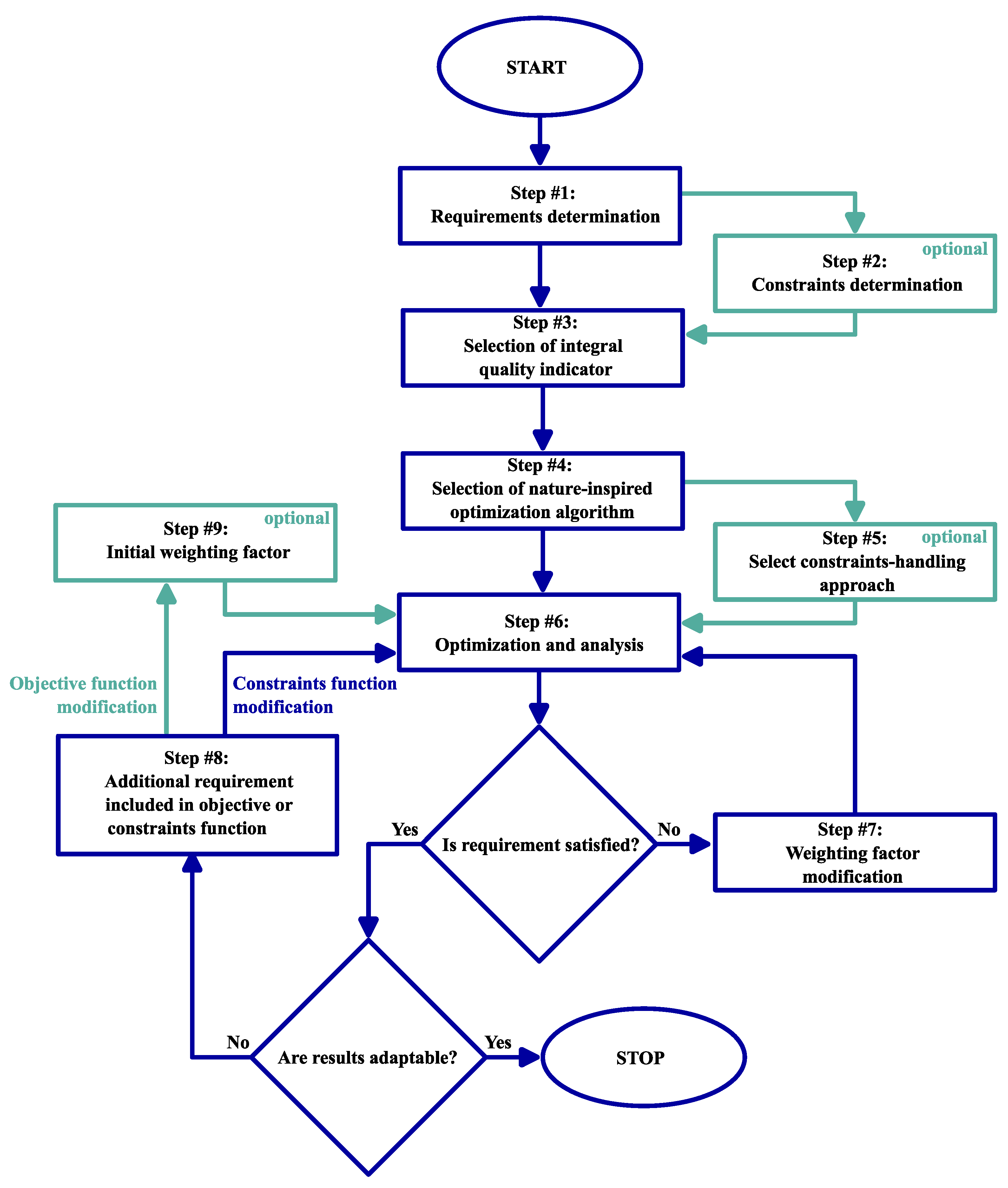
4. The Methodology

The most crucial aspect of applying a nature-inspired optimization algorithm to select optimal control structure parameters is related to determining the appropriate objective function. The task is not trivial and is related to the analyzed plant. However, a general procedure can be determined. In this section, the proposed methodology for the application of nature-inspired optimization algorithms to select optimal control structure parameters is described in detail with an example.

The procedure is performed step by step with feedback and a repetition of particular steps to achieve the predefined requirements of the output signal of the control system considered. The algorithm is as follows:

Step #1: 

Determine the requirements of the system response.

Step #2: 

(optional) Determine the constraints for the control system.

Step #3: 

Select the basic integral quality indicator, e.g., IAE Equation (2), ITSE Equation (3) (Section 2.1).

Step #4: 

Select the nature-inspired optimization algorithm.

Step #5: 

(optional) Select constraint handling approach, e.g., penalties (Section 3.2), Deb’s rules (Section 3.1).

Step #6: 

Optimize the current objective function and interpret solution. If the solution is satisfactory, the process is finished. Otherwise, continue.

Step #7: 

(optional) Modify the weighting factor and go to point 6.

Step #8: 

Include additional requirements, for example, the maximum overshoot value (see Section 2.3).

Step #9: 

Set the initial guess of the weighting factor of the new requirement and go to point 6.

The graphical representation in the form of the flow diagram of the proposed algorithm is presented in Figure 2.

4.1. An Example

For a better understanding of the proposed methodology, the following example is considered. The object is defined as a second-order system:

$$G_{\mathrm{O}\mathrm{example}}\left(s\right)={\displaystyle \frac{k{\omega }_n^2}{s^2+2\zeta {\omega }_{n}s+{\omega }_n^2}}$$

(31)

where $k=1$, $\zeta =0.5$ and ${\omega }_n=10$. The controller is a continuous-time PID:

$$G_{\mathrm{R}\mathrm{example}}=K_p+{\displaystyle \frac{K_i}{s}}+K_{d}s$$

(32)

where $K_p$, $K_i$, and $K_d$ are proportional, integral, and derivative gains, respectively. The source files can be found at Mathworks FileExchange in [32] for simulation in the Matlab environment.

4.1.1. Step #1: Requirement Determination

The requirements of the system response are as follows: the best possible performance with the predefined rise time and relatively low overshoot.

4.1.2. Step #3: Selection of Integral Quality Indicator

Therefore, the ITAE quality indicator was selected, because its minimum value is achieved for a high damping factor (see Section 2.1):

$$\mathcal{F}\left(x\right)=\mathrm{ITAE}$$

(33)

4.1.3. Step #4: Selection of Nature-Inspired Optimization Algorithm

The selection of a nature-inspired optimization algorithm is usually based on personal experience. The most important aspect is to select an algorithm that can handle constraints, if applicable. According to the no free lunch theorem, there is no best algorithm for any optimization problem. However, each nature-inspired optimization algorithm can find the global minimum. The difference is how many iterations of the algorithm is required and how many additional parameters must be selected. Many optimization algorithms are built into the Matlab environment or Python libraries. Therefore, the user should select the preferred one.

In this example, there are no constraints. Therefore, the state-of-the-art PSO optimization algorithm can be used successfully. The choice is motivated by the implementation in Matlab with automatic algorithm parameter selection.

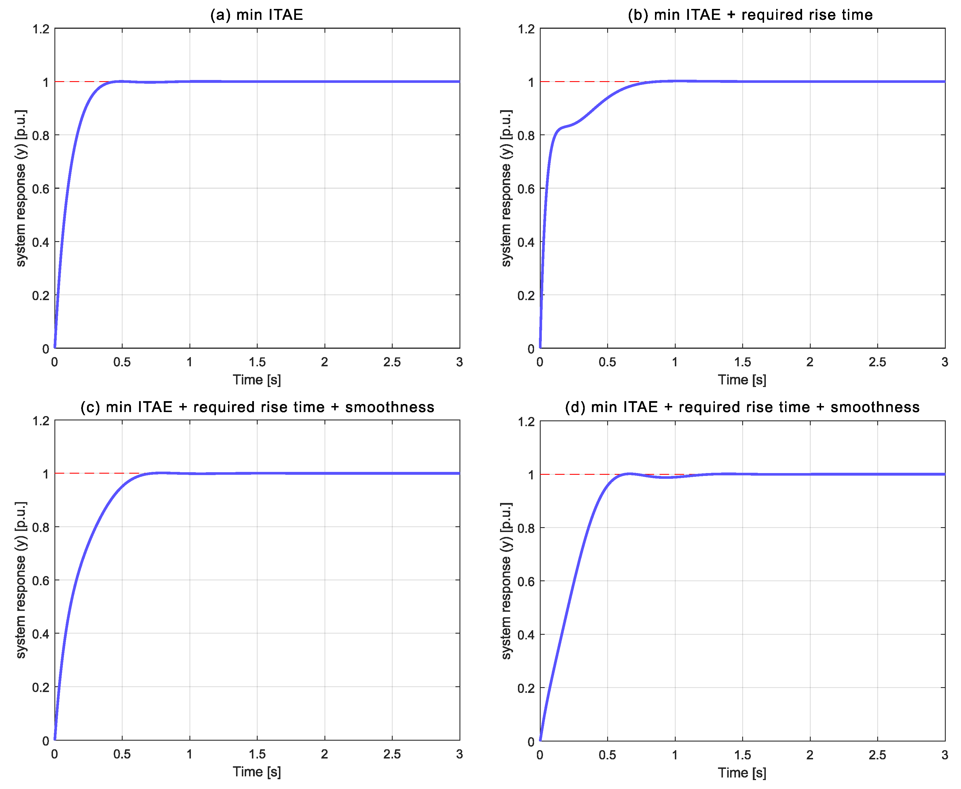
4.1.4. Step #6: Optimization and Analysis

The optimal solution for the current objective function is as follows:

$$K_p=0.92,K_i=10.0,K_d=0.094$$

$$f_{\mathrm{ITAE}}=0.0094$$

The rise time obtained is equal to $0.217$ s. The step response of the system is presented in Figure 3a. One can see that the step response is satisfactory. However, the rise time is shorter than the required rise time. Therefore, the inclusion of additional requirements into the objective function is necessary.

4.1.5. Step #8: Additional Requirement

Let us consider the required rise time equal to $0.4$ s. Therefore, the objective function is extended with the penalty function (Equation (13)), creating a multi-objective optimization problem. The determined objective function has the following form:

$$\mathcal{F}\left(x\right)=\mathrm{ITAE}+\alpha ·{\mathrm{PF}}_{\mathrm{RT}\mathrm{required}}$$

(34)

where $\alpha$ is a weighing factor, which must be determined.

4.1.6. Step #9: Initial Weighting Factor

Let us consider the accuracy of the rise time ${\mathrm{RT}}^{\mathrm{accuracy}}=25\%·{\mathrm{RT}}^{\mathrm{required}}$; then, the $\alpha$ weighting factor should be selected initially as being perfectly balance in comparison to ITAE:

$$\alpha ={\displaystyle \frac{f_{\mathrm{ITAE}}}{{\mathrm{RT}}^{\mathrm{accuracy}}}}\approx 0.09467$$

In such a case, as the difference is equal to 25% of the current rise time and the required rise time, the component related to the penalty function will have the same value as $f_{\mathrm{ITAE}}$. It is a good approximation for the initial guess of the weight factor. The optimization and analysis must be provided to ensure the weighting factor is proper.

4.1.7. Step #6: Optimization and Analysis

The optimal solution for the current objective function is as follows:

$$K_p=1.67,K_i=9.48,K_d=0.20$$

$$f_{\mathrm{ITAE}\&\mathrm{RT}}=0.0213$$

The rise time obtained is equal to $0.390$ s. One can see that the solution obtained is close to the accuracy considered. However, a higher value of the rise time provides a higher value of the ITAE indicator. Let us increase the $\alpha$ parameter.

4.1.8. Step #7: Weighting Factor Adjustment

Please, remember that the weighting factors should be as small as possible to keep the balance between the other components of the objective function. Increasing it to 10 times the previous value will force the algorithm to find a solution with an equal rise time as required, ignoring other indicators. For this reason, increase $\alpha$ by 20% as follows:

$$\alpha =1.2·{\displaystyle \frac{f_{\mathrm{ITAE}}}{{\mathrm{RT}}^{\mathrm{accuracy}}}}\approx 0.11360,$$

and repeat the optimization process.

4.1.9. Step #6: Optimization and Analysis

The optimal solution for the current objective function with an increase in $\alpha$ is as follows:

$$K_p=1.72,K_i=9.44,K_d=0.21$$

$$f_{\mathrm{ITAE}\&\mathrm{RT}}=0.0214$$

The rise time obtained is equal to $0.40$ s. The rise time value is perfectly selected to our requirement. In Figure 3b, the step response of the system is presented. Sadly, the smoothness of the output signal is not acceptable. The oscillations during the step response should be removed or minimized.

4.1.10. Step #8: Additional Requirement

To minimize the oscillations, the sum of squared derivatives of the output signal (similar to the approach presented in Equation (11)) is introduced. Therefore, the modified objective function has the following form:

$$\mathcal{F}\left(x\right)=\mathrm{ITAE}+\alpha ·{\mathrm{PF}}_{\mathrm{RT}\mathrm{required}}+\beta {\int }_0^T{\left({\displaystyle \frac{dy\left(t\right)}{dt}}\right)}^{2}dt$$

(35)

where $\beta$ is a weighing factor, T is the simulation time, and $y\left(t\right)$ is an output signal.

4.1.11. Step #9: Initial Weighting Factor

Let us considered the accuracy of the smoothness indicator as the value of

$${\mathrm{PF}}_{dy}^{\mathrm{accuracy}}={\mathrm{PF}}_{dyITAE}={\int }_0^T{\left({\displaystyle \frac{d{y}^{\mathrm{ITAE}}\left(t\right)}{dt}}\right)}^{2}dt$$

for the objective function using ITAE without additional penalties:

$$\beta ={\displaystyle \frac{f_{\mathrm{ITAE}\&\mathrm{RT}}}{{\mathrm{PF}}_{dy}^{\mathrm{accuracy}}}}\approx 4.48$$

4.1.12. Step #6: Optimization and Analysis

The optimal solution for the current objective function with an additional component and weighting factor ($\beta$) is as follows:

$$K_p=0.53,K_i=5.90,K_d=0.071$$

$$f_{\mathrm{ITAE}\&\mathrm{RT}\&\mathrm{smoothness}}=0.041$$

The obtained rise time is equal to $0.40$ s, which is the required value. In addition, the smoothness has been significantly improved, from the value ${\mathrm{PF}}_{dy}=0.0091$ to ${\mathrm{PF}}_{dy}=0.0030$. The step response of the system is presented in Figure 3c. The selected weighting factor can be decreased or increased to improve the output signal of the considered system. Let us increase its value to force the algorithm to provide a smoother system response.

4.1.13. Step #7: Weighting Factor Adjustment

For example, let us increase it ten times to show its impact on the final solution:

$$\beta =10·{\displaystyle \frac{f_{\mathrm{ITAE}\&\mathrm{RT}}}{{\mathrm{PF}}_{dy}^{\mathrm{accuracy}}}}\approx 44.8$$

4.1.14. Step #6: Optimization and Analysis

The optimal solution for the current objective function for the increased weighting factor value $\beta$ is as follows:

$$K_p=0.22,K_i=4.48,K_d=0.034$$

$$f_{\mathrm{ITAE}\&\mathrm{RT}\&\mathrm{smoothness}}=0.131$$

The obtained rise time is still equal to $0.40$ s and the smoothness is improved to $0.0020$. The step response of the system is presented in Figure 3d.

One can see that the smoothness indicator is improved, but the response of the system is more oscillating compared to the previous weighting factor value ($\beta$). Therefore, the final result obtained for an initial guess of $\beta$ is satisfactory and the process is finished with the result presented in Figure 3c.

5. Case Studies

In this section, two examples are considered. Each represents a different control structure, plant, and approach for formulating the objective function. Hysteresis and PID controllers are considered in terms of control structure. These control structures control the heating system and the DC motor, respectively. The objective functions are formulated to present requirements, penalties, and constraints. Therefore, case studies should be analyzed with particular emphasis on approaches to formulating the proper objective and constraint functions.

In the first example, the particle swarm optimization algorithm was used. To show that the other nature-inspired optimization algorithms are also eligible for application, the artificial bee colony optimization algorithm was used in the following case studies. However, most of the nature-inspired optimization algorithms can solve analyzed problems. The selection of the optimization algorithm is related to the authors’ experience applying the ABC algorithm to different optimization problems. In the previous papers, the authors compared artificial bee colony algorithm to other nature-inspired optimization algorithms [12]. The conclusions can be summarized as follows: all of the examined optimization algorithms allow us to reach the satisfactory solution. However, the time required to find the global minimum differs significantly. The comparison and in-depth review of nature-inspired optimization algorithms can be found in [33,34].

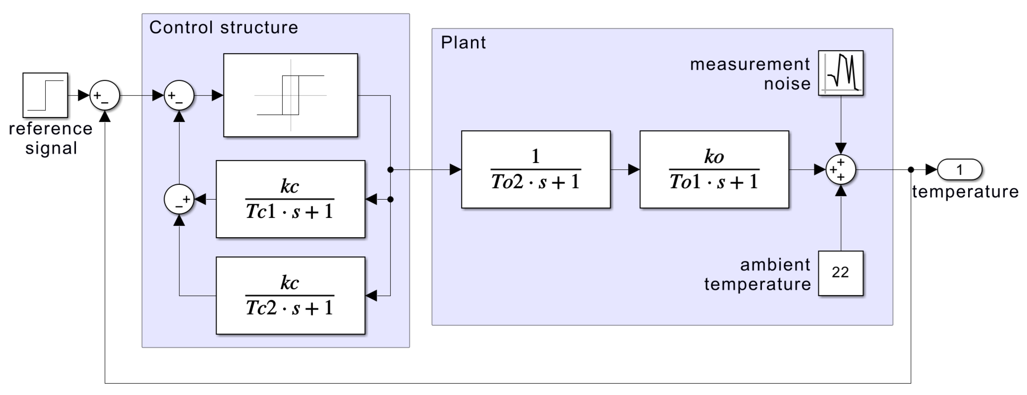
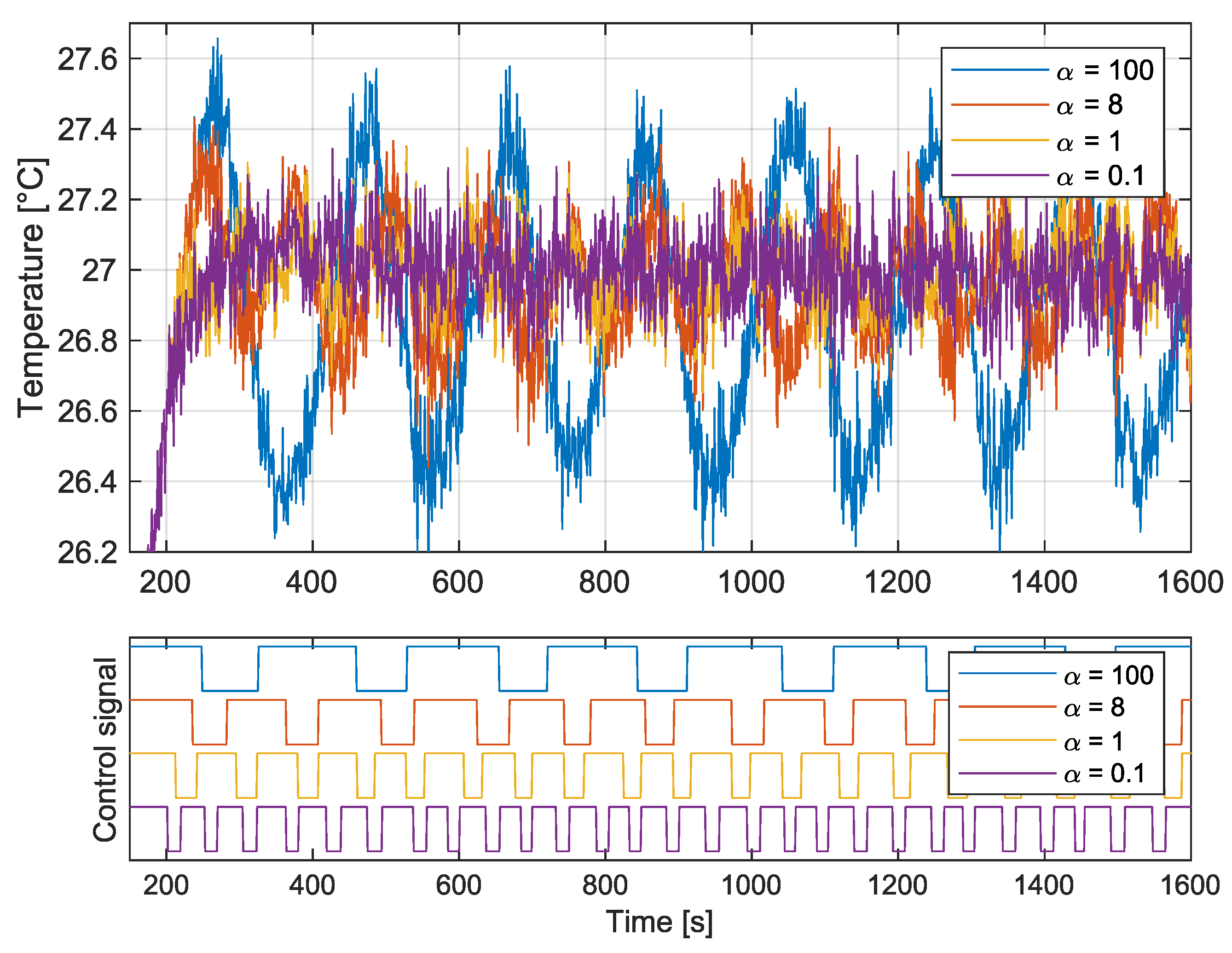
5.1. Hysteresis Control with PID Correction for Temperature Control

In the first example, the heating system is considered. It was selected as an example of a non-linear plant. Moreover, the requirement of such a control structure can be simply determined: minimize the oscillations in a quasi-steady state and minimize the switching frequency. The considered heating system, described in the form of the transfer function, is as follows:

$$G_{\mathrm{plant}}\left(s\right)={\displaystyle \frac{k_o}{(T_{o1}s+1)(T_{o2}s+1)}}$$

(36)

where k is the static gain of the plant, and $T_{o1}$ and $T_{o2}$ are time constants. The output signal is the temperature, while the control signal is the heater state. Due to the consideration of a discontinuous control signal, i.e., on/off output state, the hysteresis controller is used. To obtain higher system performance, the PID correction method can be used.The hysteresis controller is covered by two additional close loops with the following transmutations:

$$G_{c1}\left(s\right)={\displaystyle \frac{k_c}{T_{c1}s+1}}$$

(37)

$$G_{c2}\left(s\right)={\displaystyle \frac{k_c}{T_{c2}s+1}}$$

(38)

where $k_c$, $T_{c1}$ and $T_{c2}$ are PID correction parameters. The general block diagram of the system is presented in Figure 4. The parameters of the control system are listed in

Table 2. Parameters of the heating system.

Parameter	Value
Static gain of the plant ($k_o$)	7.5 °C/V
Time constant of the plant ($T_{o1}$)	150 s
Time constant of the plant ($T_{o2}$)	50 s
Hysteresis value (H)	1 °C

.

Note that measurement noise was added to the plant’s output to increase the impact of PID correction on system performance.

5.1.1. Proposed Objective Function

Note that the main objective of the considered example is to provide a lower error between the reference and the current temperature. An ISE indicator is proposed to minimize the control loop error in this case. On the other hand, the hysteresis controller commonly uses the electronic relay. Therefore, the number of switches should be minimized to ensure long-term operation of the system without maintenance. If the ISE indicator is minimized, the number of changes in the relay state increases the overall value of the objective function as a punishment. The objective function for the considered hysteresis control with PID correction for temperature control is as follows:

$$F_{\mathrm{heater}}=\sum _{k=0}^N{\left(y^{\mathrm{ref}}-y\left(k\right)\right)}^2·T_s+\alpha \sum _{k=0}^N\Delta u\left(k\right)$$

(39)

with

$$\Delta u\left(k\right)=\left\{\begin{array}{cc}1,& \mathrm{if}u \& (k-1)=0u\left(k\right)=1\hfill \\ 0,& \mathrm{otherwise}\hfill \end{array}\right.$$

where N is the number of samples per experiment; $y^{\mathrm{ref}}$ and y are reference and current temperature, respectively; $T_s$ is the sampling period; $\alpha$ is a weighting factor; u is a state of the hysteresis controller; and $\Delta u$ is used to count the rising edges of the control signal.

5.1.2. Results

To minimize the proposed objective function given by Equation (39), the artificial bee colony optimization algorithm was used. Figure 5 presents the plot obtained for different values of the weighting factor $\alpha$, while

Table 3. Results of hysteresis PID correction coefficients for the proposed objective function with different values of the $\alpha$ coefficient.

$\mathit{\alpha }$	$\sum \Delta \mathit{u}$	ISE	${\mathit{k}}_{\mathit{c}}$	${\mathit{T}}_{\mathit{c}1}$	${\mathit{T}}_{\mathit{c}2}$
0.1	58	$2.54\times {10}^3$	7.12	57.0	100
1	40	$2.55\times {10}^3$	8.96	69.5	93.6
8	25	$2.60\times {10}^3$	3.29	59.6	92.5
100	15	$2.92\times {10}^3$	0.1	100	47.2

presents the numerical indicators.

One can see that the proposed objective function minimizes the oscillations in the quasi-steady state and simultaneously minimizes the control signal’s switching frequency. The proposed objective function successfully met the above-discussed assumptions. The balance between these two requirements can be determined by properly selecting the weighting factor $\alpha$. Unfortunately, in such an objective function, the value of the switching frequency cannot be easily determined. Therefore, the weighting factor $\alpha$ has to be selected using a trial-and-error approach.

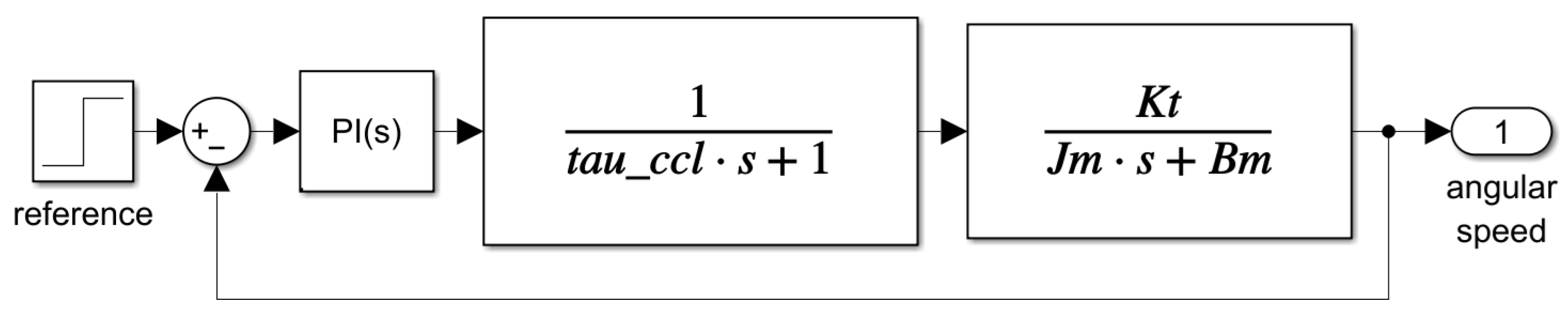
5.2. Proportional–Integral Speed Controller for DC Motor

The second example presents the automatic tuning of the most commonly used controller, the proportional–integral (PI) controller. The speed control of the DC motor is considered. In such a system, the step response of the speed will be determined using step response indicators. Therefore, the required overshoot and the required rise time will be used to formulate the objective function.

5.2.1. Mathematical Formulation

To simplify the mathematical description, the torque control loop is modeled as the first-order system:

$$G_{\mathrm{DC}TCL}\left(s\right)={\displaystyle \frac{T_e\left(s\right)}{T_e^{\mathrm{ref}}\left(s\right)}}={\displaystyle \frac{K_t}{{\tau }_{CCL}s+1}}$$

(40)

where $T_e\left(s\right)$ and $T_e^{ref}\left(s\right)$ are the torque generated by the motor and the reference value, respectively, ${\tau }_{CCL}$ is the time constant of the current control loop, and $K_t$ is the torque constant of the DC motor. Next, the mechanical equation can be modeled using a moment of inertia ($J_m$) and a viscous friction ($B_m$):

$$G_{\mathrm{DC}m}\left(s\right)={\displaystyle \frac{{\mathrm{\Omega }}_m\left(s\right)}{T_e\left(s\right)}}={\displaystyle \frac{1}{J_{m}s+B_m}}$$

(41)

where ${\mathrm{\Omega }}_m\left(s\right)$ is the angular speed of the motor. Finally, the plant can be written as

$$G_{\mathrm{DC}}\left(s\right)={\displaystyle \frac{{\mathrm{\Omega }}_m\left(s\right)}{T_e^{\mathrm{ref}}\left(s\right)}}=G_{\mathrm{DC}TCL}\left(s\right)·G_{\mathrm{DC}m}\left(s\right)$$

(42)

As mentioned earlier, the PI controller will be used to control the speed loop of the DC motor. Assuming that the system operates in a linear range, the transfer function of the PI controller is as follows:

$$G_{\mathrm{PI}}\left(s\right)={\displaystyle \frac{T_e^{\mathrm{ref}}\left(s\right)}{{\mathrm{\Omega }}_m^{\mathrm{ref}}\left(s\right)-{\mathrm{\Omega }}_m\left(s\right)}}=K_p+{\displaystyle \frac{1}{T_{i}s}}$$

(43)

where $K_p$ and $T_i$ are parameters of the PI controller that will be optimized to minimize the objective function. The block diagram of the control system is presented in Figure 6, while the parameters used are listed in

Table 4. Parameters of the DC drive systems.

Parameter	Value
Current control loop time constant (${\tau }_{CCL}$)	0.001 s
Torque constant ($K_t$)	1 Nm/A
Moment of inertia ($J_m$)	1 × 10−4 kg·m2
Viscous friction coefficient ($B_m$)	4 × 10−5 Nm·s/rad

.

5.2.2. Proposed Objective Function

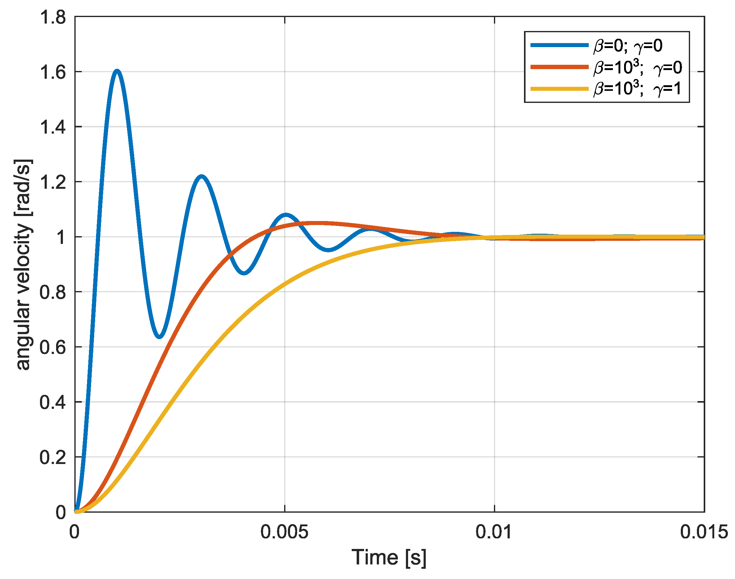
Firstly, to ensure that steady-state errors do not occur, the ITSE quality indicator will be used. Secondly, the maximum overshoot (${\mathrm{SI}}_{\mathrm{PO}}^{\mathrm{limit}}$) and the required rise time (${\mathrm{SI}}_{\mathrm{RT}}^{\mathrm{required}}$) are defined as follows:

$${\mathrm{SI}}_{\mathrm{PO}}^{\mathrm{DC}}\approx {\mathrm{SI}}_{\mathrm{PO}}^{\mathrm{limit}}$$

(44)

$${\mathrm{SI}}_{\mathrm{RT}}^{\mathrm{DC}}\approx {\mathrm{SI}}_{\mathrm{RT}}^{\mathrm{required}}$$

(45)

Therefore, the objective function is defined as follows:

$$\begin{array}{cc}\hfill F_{\mathrm{DC}}=& \sum _{k=0}^{N}k{T}_s{\left({\omega }_m^{\mathrm{ref}}-{\omega }_m\left(k\right)\right)}^2·T_s\hfill \\ \hfill & +\beta ·max\left({\mathrm{SI}}_{\mathrm{PO}}^{\mathrm{DC}}-{\mathrm{SI}}_{\mathrm{PO}}^{\mathrm{limit}},0\right)\hfill \\ \hfill & +\gamma ·\left|{\mathrm{SI}}_{\mathrm{RT}}^{\mathrm{DC}}-{\mathrm{SI}}_{\mathrm{RT}}^{\mathrm{required}}\right|\hfill \end{array}$$

(46)

where $\beta$ and $\gamma$ are weighting factors. It should be noted that $\beta$ is responsible for limiting the overshoot. Therefore, it should be a relatively high value to reject the solution if the overshoot exceeds. Due to usage of MAX, the expression can be analyzed as a discrete value equal to 0 (criterion Equation (44) fulfilled) or ∞ (criterion Equation (44) unfulfilled). On the other hand, the weighting factor $\gamma$ determines the importance of the ITSE part of the objective function and the rise time requirement.

5.2.3. Results

Figure 7 presents the step responses obtained for different values of the weighting factors $\beta$ and $\gamma$, while

Table 5. Step response quality indicators of speed control using PI controller obtained with different values of $\beta$ and $\gamma$ coefficients.

$\mathit{\beta }$	$\mathit{\gamma }$	ITSE	${\mathbf{SI}}_{\mathbf{PO}}^{\mathbf{DC}}$	${\mathbf{SI}}_{\mathbf{RT}}^{\mathbf{DC}}$	${\mathit{K}}_{\mathit{p}}$	${\mathit{T}}_{\mathit{i}}$
0	0	$4.98\times {10}^{-7}$	60.3%	$3.7\times {10}^{-4}$ s	10	10
${10}^3$	0	$1.37\times {10}^{-6}$	5.0%	$28.0\times {10}^{-4}$ s	0.546	1.748
${10}^3$	1	$2.96\times {10}^{-6}$	0.04%	$50.0\times {10}^{-4}$ s	0.319	0.954

presents the step response indicators and the PI controller parameters obtained. The weighting factors were selected to present the result for the ITSE indicator ($\beta =\gamma =0$), ITSE indicator with overshoot limited ($\beta ={10}^3,\gamma =0$), and additional requirement to reach the required rise time ($\beta ={10}^3,\gamma ={10}^{-3}$).

The first experiment with zero values of $\beta$ and $\gamma$ is an objective function using only the ITSE indicator. In such a case, huge overshoots and oscillations occur. Next, the value $\beta$ was set at a relatively high value to limit the percentage overshoot to the assumed value (equal to 5%). One can see that the proposed objective function successfully limits the overshoot. It should be noted that reducing the overshoot also reduces the rise time. Increasing the weighting factor $\gamma$ allows one to define the required rise time.

6. Conclusions

Today, the application of nature-inspired optimization algorithms for an optimal selection of control structure parameters is common. This paper discussed the automatic selection of control structure parameters using a nature-inspired optimization algorithm. The authors presented and discussed possibilities for quality control indicators, the creation of an objective function, and weighting factor impacts. Moreover, the methodology of the application of nature-inspired optimization algorithms was proposed to select the optimal parameters of the control structure. The proposed algorithm was discussed in depth on a simple example published in the open source repository. It is worth pointing out the universality of the proposed approach. The number of parameters in the control structure is not important from the point of view of the proposed methodology. The higher dimensionality problem requires a higher computational effort; however, from a practical point of view, user-friendly requirements like step response indicators are an important advantage of the proposed method. However, for a very high number of parameters, the optimization algorithm can require many hours or even days. The case studies summarize the theoretical aspect of this research paper. A simple example is presented allow readers to understand the crucial aspects of the automatic tuning mechanism using nature-inspired optimization algorithms. The impact of the weighting factor was presented and discussed.

References

1. Sahu, B.K.; Pati, S.; Mohanty, P.K.; Panda, S. Teaching–learning based optimization algorithm based fuzzy-PID controller for automatic generation control of multi-area power system. Appl. Soft Comput. 2015, 27, 240–249. [Google Scholar] [CrossRef]
2. Solihin, M.I.; Wahyudi; Kamal, M.; Legowo, A. Optimal PID controller tuning of automatic gantry crane using PSO algorithm. In Proceedings of the 2008 5th International Symposium on Mechatronics and Its Applications, Amman, Jordan, 27–29 May 2008; IEEE: Piscataway, NJ, USA, 2008; pp. 1–5. [Google Scholar]
3. He, Y.; Zhou, Y.; Wei, Y.; Luo, Q.; Deng, W. Wind driven butterfly optimization algorithm with hybrid mechanism avoiding natural enemies for global optimization and PID controller design. J. Bionic Eng. 2023, 20, 2935–2972. [Google Scholar] [CrossRef]
4. Patil, R.S.; Jadhav, S.P.; Patil, M.D. Review of Intelligent and Nature-Inspired Algorithms-Based Methods for Tuning PID Controllers in Industrial Applications. J. Robot. Control JRC 2024, 5, 336–358. [Google Scholar] [CrossRef]
5. Malarczyk, M.; Katsura, S.; Kaminski, M.; Szabat, K. A Novel Meta-Heuristic Algorithm Based on Birch Succession in the Optimization of an Electric Drive with a Flexible Shaft. Energies 2024, 17, 4104. [Google Scholar] [CrossRef]
6. Tarczewski, T.; Stojic, D.; Dzielinski, A. Large Language Model-Based Tuning Assistant for Variable Speed PMSM Drive with Cascade Control Structure. Electronics 2025, 14, 232. [Google Scholar] [CrossRef]
7. Sahu, R.K.; Panda, S.; Rout, U.K.; Sahoo, D.K. Teaching learning based optimization algorithm for automatic generation control of power system using 2-DOF PID controller. Int. J. Electr. Power Energy Syst. 2016, 77, 287–301. [Google Scholar] [CrossRef]
8. Niewiara, Ł.J.; Szczepański, R.; Tarczewski, T.; Grzesiak, L.M. State feedback speed control with periodic disturbances attenuation for PMSM drive. Energies 2022, 15, 587. [Google Scholar] [CrossRef]
9. Tarczewski, T.; Niewiara, Ł.J.; Grzesiak, L.M. Application of artificial bee colony algorithm to auto-tuning of state feedback controller for DC-DC power converter. Power Electron. Drives 2016, 1, 83–96. [Google Scholar]
10. Szczepanski, R.; Kaminski, M.; Tarczewski, T. Auto-tuning process of state feedback speed controller applied for two-mass system. Energies 2020, 13, 3067. [Google Scholar] [CrossRef]
11. Szczepanski, R.; Tarczewski, T.; Erwinski, K.; Grzesiak, L.M. Comparison of Constraint-handling Techniques Used in Artificial Bee Colony Algorithm for Auto-Tuning of State Feedback Speed Controller for PMSM. In Proceedings of the 15th International Conference on Informatics in Control, Automation and Robotics, Portu, Portugal, 29–31 July 2018; pp. 279–286. [Google Scholar]
12. Tarczewski, T.; Stojic, D.; Szczepanski, R.; Niewiara, L.; Grzesiak, L.M.; Hu, X. Online auto-tuning of multiresonant current controller with nature-inspired optimization algorithms and disturbance in the loop approach. Appl. Soft Comput. 2023, 144, 110512. [Google Scholar] [CrossRef]
13. Zychlewicz, M.; Stanislawski, R.; Kaminski, M. Grey wolf optimizer in design process of the recurrent wavelet neural controller applied for two-mass system. Electronics 2022, 11, 177. [Google Scholar] [CrossRef]
14. Łapa, K.; Cpałka, K. Flexible fuzzy PID controller (FFPIDC) and a nature-inspired method for its construction. IEEE Trans. Ind. Inform. 2017, 14, 1078–1088. [Google Scholar]
15. Benitez-Garcia, S.E.; Villarreal-Cervantes, M.G.; Mezura-Montes, E. Event-triggered control optimal tuning through bio-inspired optimization in robotic manipulators. ISA Trans. 2022, 128, 81–105. [Google Scholar] [CrossRef] [PubMed]
16. Du, C.; Yin, Z.; Zhang, Y.; Liu, J.; Sun, X.; Zhong, Y. Research on active disturbance rejection control with parameter autotune mechanism for induction motors based on adaptive particle swarm optimization algorithm with dynamic inertia weight. IEEE Trans. Power Electron. 2018, 34, 2841–2855. [Google Scholar] [CrossRef]
17. Bassi, S.; Mishra, M.; Omizegba, E.E. Automatic tuning of proportional-integral-derivative (PID) controller using particle swarm optimization (PSO) algorithm. Int. J. Artif. Intell. Appl. 2011, 2, 25. [Google Scholar] [CrossRef]
18. Sun, X.; Hu, C.; Lei, G.; Guo, Y.; Zhu, J. State feedback control for a PM hub motor based on gray wolf optimization algorithm. IEEE Trans. Power Electron. 2019, 35, 1136–1146. [Google Scholar] [CrossRef]
19. Kaminski, M. Nature-inspired algorithm implemented for stable radial basis function neural controller of electric drive with induction motor. Energies 2020, 13, 6541. [Google Scholar] [CrossRef]
20. Jumani, T.A.; Mustafa, M.W.; Hussain, Z.; Rasid, M.M.; Saeed, M.S.; Memon, M.M.; Khan, I.; Nisar, K.S. Jaya optimization algorithm for transient response and stability enhancement of a fractional-order PID based automatic voltage regulator system. Alex. Eng. J. 2020, 59, 2429–2440. [Google Scholar] [CrossRef]
21. Gozde, H. Robust 2DOF state-feedback PI-controller based on meta-heuristic optimization for automatic voltage regulation system. ISA Trans. 2020, 98, 26–36. [Google Scholar] [CrossRef]
22. Tarczewski, T.; Grzesiak, L.M. An application of novel nature-inspired optimization algorithms to auto-tuning state feedback speed controller for PMSM. IEEE Trans. Ind. Appl. 2018, 54, 2913–2925. [Google Scholar] [CrossRef]
23. Ufnalski, B.; Kaszewski, A.; Grzesiak, L.M. Particle swarm optimization of the multioscillatory LQR for a three-phase four-wire voltage-source inverter with an LC output filter. IEEE Trans. Ind. Electron. 2014, 62, 484–493. [Google Scholar] [CrossRef]
24. Fister, D.; Fister, I., Jr.; Fister, I.; Šafarič, R. Parameter tuning of PID controller with reactive nature-inspired algorithms. Robot. Auton. Syst. 2016, 84, 64–75. [Google Scholar] [CrossRef]
25. Micev, M.; Ćalasan, M.; Ali, Z.M.; Hasanien, H.M.; Aleem, S.H.A. Optimal design of automatic voltage regulation controller using hybrid simulated annealing–Manta ray foraging optimization algorithm. Ain Shams Eng. J. 2021, 12, 641–657. [Google Scholar] [CrossRef]
26. Coutinho, J.P.; Santos, L.O.; Reis, M.S. Bayesian Optimization for automatic tuning of digital multi-loop PID controllers. Comput. Chem. Eng. 2023, 173, 108211. [Google Scholar] [CrossRef]
27. Cao, J.; Sun, X.; Tian, X. Optimal control strategy of state feedback control for surface-mounted PMSM drives based on auto-tuning of seeker optimization algorithm. Int. J. Appl. Electromagn. Mech. 2021, 66, 705–725. [Google Scholar] [CrossRef]
28. Aguilar-Mejía, O.; Minor-Popocatl, H.; Tapia-Olvera, R. Comparison and Ranking of Metaheuristic Techniques for Optimization of PI Controllers in a Machine Drive System. Appl. Sci. 2020, 10, 6592. [Google Scholar] [CrossRef]
29. Eberhard, P.; Sedlaczek, K. Using Augmented Lagrangian Particle Swarm Optimization for Constrained Problems in Engineering. In Advanced Design of Mechanical Systems: From Analysis to Optimization; Springer: Vienna, Austria, 2009; pp. 253–271. [Google Scholar] [CrossRef]
30. Birgin, E.G.; Martinez, J.M. Improving ultimate convergence of an augmented Lagrangian method. Optim. Methods Softw. 2008, 23, 177–195. [Google Scholar] [CrossRef]
31. Andreani, R.; Birgin, E.G.; Martínez, J.M.; Schuverdt, M.L. On augmented Lagrangian methods with general lower-level constraints. SIAM J. Optim. 2008, 18, 1286–1309. [Google Scholar] [CrossRef]
32. Szczepanski, R. An Example of Automatic Tuning of Controller Parameters. MATLAB Central File Exchange. 2025. Available online: https://www.mathworks.com/matlabcentral/fileexchange/181202-an-example-of-automatic-tuning-of-controller-parameters (accessed on 29 May 2025).
33. Yang, X.S. Nature-Inspired Optimization Algorithms; Academic Press: Cambridge, MA, USA, 2020. [Google Scholar]
34. Kumar, A.; Nadeem, M.; Banka, H. Nature inspired optimization algorithms: A comprehensive overview. Evol. Syst. 2023, 14, 141–156. [Google Scholar] [CrossRef]
Figure 1. Impact of damping factor ( ζ ) in second-order system on basic quality indicators.
Asi 08 00079 g001
Figure 2. The flow diagram of the proposed algorithm.
Asi 08 00079 g002
Figure 3. Optimization result obtained for an analyzed example.
Asi 08 00079 g003
Figure 4. Control scheme of hysteresis control with PID correction for temperature control.
Asi 08 00079 g004
Figure 5. Results of hysteresis PID correction coefficients for the proposed objective function with different values of the α coefficient.
Asi 08 00079 g005
Figure 6. Control scheme of PI speed controller for DC drive.
Asi 08 00079 g006
Figure 7. Step response of speed control using PI controller obtained with different values of β and γ coefficients.
Asi 08 00079 g007