Abstract
This study focuses on the remotely operated underwater vehicle (ROV) and addresses key issues in existing simulation systems, such as neglecting the influence of ocean currents on the ROV’s trajectory or only simulating the impact of ocean currents instead of combining wake flow and ocean currents. Additionally, the visualization capabilities of current simulation systems still have room for improvement. This paper develops a three-dimensional path simulation system for ocean inspection robots to tackle these challenges based on MATLAB and Simulink. The system optimizes the drag matrix of the original simulation model by decomposing the sea current into three directional components in three-dimensional space and simulating the relative velocity in each direction separately; it introduces the influence of the current wake, thus more accurately realizing the trajectory simulation of the ROV under the current perturbation. Experimental results demonstrate high consistency between the optimized model’s simulation outcomes and theoretical expectations. The proposed system significantly improves trajectory evolution stability and consistency, compared to traditional models. The findings of this study indicate that the proposed optimized simulation system not only effectively verifies the applicability of control algorithms but also provides reliable data support for ROV design and optimization. Additionally, it lays a solid foundation for further developing intelligent underwater robots based on Internet of Things (IoT) technology.
1. Introduction
In recent years, the global underwater robotics market has been experiencing rapid growth (Figure 1). Underwater robots have a wide range of applications and significant market demand in fields such as deep-sea exploration, aquaculture, and marine engineering [1]. Currently, a variety of robots have been developed that can operate at different depths and perform multiple tasks, including oil extraction, seabed mineral surveys, salvage operations, pipeline laying and inspection, cable installation and inspection, offshore aquaculture, dam inspections in rivers and reservoirs, and military applications [2]. Underwater robots are increasingly vital in military and civilian sectors, among which autonomous navigation and path planning are considered core technologies.
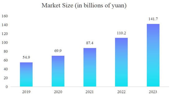
Figure 1.
Global underwater robotics market size.
A significant body of research has focused on the path planning and simulation of underwater robots, with particular emphasis on enhancing performance in complex marine environments. A deep-sea condition-based simulation system has been developed to replicate underwater scenarios, highlighting the importance of intelligent path planning for improving operational efficiency [3]. However, such systems often assume simplified current fields and do not integrate high-fidelity control or close-range hydrodynamic effects, which limits their predictive capability in dynamic environments. A six-degrees-of-freedom underwater robot model has been proposed to track moving targets, offering high precision and incorporating ocean current effects; however, it is limited to tracking along fixed linear paths and does not account for wake flow during close-range maneuvers, reducing its applicability in dynamic settings [4], which are especially critical during docking, inspection, or other operations that require precise proximity control. The genetic algorithm-based simulation framework considers automatic obstacle avoidance and two-dimensional ocean current influence, yet it remains constrained to planar analysis, omitting the impact of three-dimensional current disturbances and wake effects on trajectory accuracy [5], limiting its applicability in complex ocean environments where vertical current gradients and vortex shedding significantly affect vehicle stability. Another model integrates path planning in ocean environments but lacks support for three-dimensional current simulations, thus failing to provide robust trajectory optimization for real-world deployment [6]. While effective in route optimization, this model abstracts away from physical hydrodynamics and fails to simulate near-field flow interactions needed for real-time control. Force and motion data of a tethered ROV operating under combined wave and current conditions have been presented to provide a reliable benchmark for validating numerical simulation methods [7]. The fixed structure cannot support trajectory tracking or adaptive control in unstructured flow fields. However, the fixed configuration of the ROV in this setup limits its applicability to scenarios requiring real-time control and unrestricted movement. A computational fluid dynamics (CFD)-based modeling approach has also been employed to analyze hydrodynamic forces on ROVs under varying current speeds and flow directions [8], suggesting that similar hybrid techniques could be adapted to underwater domains, especially for real-time trajectory tuning in turbulent fields. Nevertheless, this method lacks integration with trajectory tracking and closed-loop control mechanisms. In a related domain, an aerodynamic optimization method has been proposed for reducing drag on vehicle surfaces using CFD in combination with machine learning and genetic algorithms [9]. Although applied in an atmospheric environment, this approach highlights the potential of simulation-driven optimization strategies for improving underwater trajectory planning in complex flow fields.
Based on the deficiencies in path planning for underwater robots mentioned above, this paper proposes an optimized simulation model for underwater robots under the influence of three-dimensional ocean currents by considering the interference of ocean currents and introducing the influence of wake currents simultaneously, based on previous research results. The model allows the user to specify the currents in a particular region, set the size, and then observe how the trajectory of the six-degrees-of-freedom ROV model is affected by the currents and wake flows while moving close to the target, which makes it easy for the user to re-specify the route or analyze the data.
2. Extension and Refinement of the Ocean Disturbance Simulation System Model
To achieve precise modeling and control of underwater vehicle motion in the presence of complex ocean current disturbances, it is essential to construct a comprehensive simulation framework that integrates both physical dynamics and control logic. This section presents the theoretical underpinnings of the proposed ocean disturbance simulation system. By leveraging the MATLAB/Simulink environment, the framework establishes a closed-loop control structure composed of five interrelated functional modules. Each module plays a critical role in accurately simulating the real-time behavior of underwater vehicles under hydrodynamic forces and control feedback, thereby ensuring the fidelity and robustness of the simulation system.
2.1. Theoretical Basis
The proposed method established a closed-loop framework within the MATLAB/Simulink environment to enable accurate motion control and dynamic simulation under ocean current disturbances. The system architecture comprised four interdependent modules—Kinetics, Kinematics, Controller, and Allocation—constituting an underwater vehicle’s fully integrated motion control and simulation loop [10]. The functional descriptions of each module are as follows.
- 1.
- Kinetics Module
The Kinetics module models the dynamic behavior of the underwater vehicle by solving the six-degrees-of-freedom (6-DOF) Newton–Euler equations of motion. It receives external force and moment inputs τ and ocean current disturbances v and computes the linear and angular accelerations of the vehicle. The dynamic model includes an inertia matrix M, a Coriolis and centripetal matrix C(ν), a hydrodynamic damping matrix D, and a restoring force vector G(η), all contributing to a physically realistic simulation. The resulting accelerations are passed to the Kinematics module for further processing.
- 2.
- Kinematics Module
This module estimates the real-time status of the robot, including position, velocity, and orientation (i.e., roll, pitch, and yaw angles). It integrates the accelerations provided by the Kinetics module to derive the vehicle’s motion trajectory in the global frame. The module also accounts for initial pose conditions and continuously updates the robot’s motion states throughout the simulation [11]. The resulting kinematic information is then forwarded to the Controller module to support closed-loop control [12].
- 3.
- Controller Module
The Controller module is the decision-making center of the system. It compares the real-time motion states from the Kinematics module with the desired trajectory and orientation. Based on the computed tracking errors, it employs control strategies—such as proportional–integral–derivative (PID) control or advanced nonlinear control algorithms—to generate control inputs u. These inputs represent the desired generalized forces and moments needed to correct the robot’s trajectory and are passed to the Allocation module [13].
- 4.
- Allocation Module
The Allocation module decomposes the control inputs u into actuator-level commands. Utilizing a predefined thrust allocation matrix T and actuator calibration matrix K, it computes the required thrust for each thruster such that the resultant forces and moments match the global control objectives. This module ensures effective resource distribution and minimizes control errors due to actuator constraints. The computed thrust commands are passed to the Thruster module for implementation.
- 5.
- Thruster Module
The Thruster module acts as the actuator interface. It is responsible for transforming the individual thruster commands into a combined force/moment vector τ applied to the vehicle in six degrees of freedom. The module can compute the net force and moment exerted by all thrusters using the thruster configuration model, considering their positions, orientations, and operational characteristics [14]. The output τ is then used by the Kinetics module to update the robot’s motion dynamics, thereby closing the simulation loop.
In this paper, the dynamic model of the underwater vehicle is established based on the Newton–Euler equation.
The dynamic model of the underwater robot is defined as follows:
τ is the external input control force and moment;
ν ∈ R6 denotes the velocity vector of the underwater vehicle expressed in the body-fixed frame. It is composed of three linear velocity components (u, v, w) and three angular velocity components (p, q, r):
v = [u, v, w, p, q, r]T,
denotes the time derivative of v.
The forms of each matrix are expanded as follows.
- Inertia matrix M
The inertia matrix M = MR + MA consists of two parts:
MR: inertia term composed of rigid body mass and rotational inertia;
MA: the added mass matrix accounting for the fluid-induced inertial effects due to the hydrodynamic coupling between the vehicle and the surrounding water.
The complete form is as follows. The body-fixed coordinate system is defined with its origin located at the vehicle’s center of gravity (CoG). The x-axis points forward, the y-axis points to the starboard, and the z-axis points downward, following the standard right-hand convention.
In the following matrix, m denotes the mass of the ROV. Ix, Iy, and Iz represent the moments of inertia about the roll, pitch, and yaw axes, respectively. The coordinate system used for defining these quantities is illustrated in Figure 2. MA is the additional mass term; and , and are the added mass coefficients on the three directions of freedom, respectively. The terms such as Zg, Zw, and similar off-diagonal components reflect the coupling effects arising from the offset between the center of gravity (CoG) and the center of buoyancy (CoB).
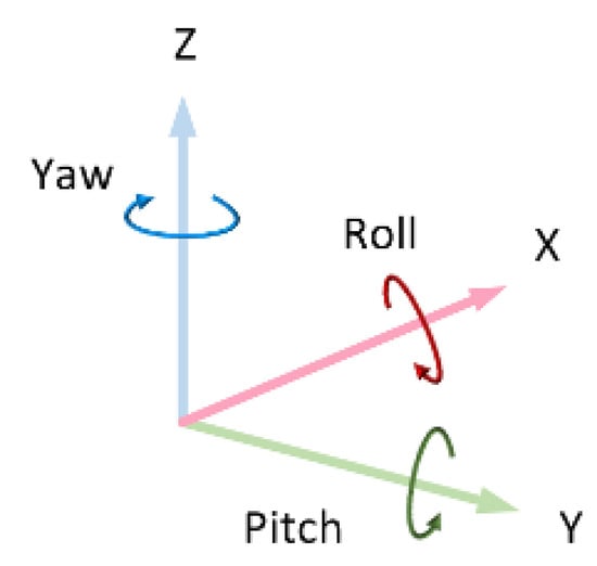
Figure 2.
The coordinate system.
Specifically, (xg, yg, zg) represents the coordinates of the CoG, which is the point where the total gravitational force is considered to act. These coordinates are determined by the mass distribution of the vehicle.
(xb, yb, zb) denotes the coordinates of the CoB, which is the centroid of the displaced fluid volume and the point where the buoyant force acts. These coordinates depend on the geometry and submerged volume of the vehicle.
Therefore, M can be expressed as follows:
- Coriolis moment matrix C(v)
This matrix reflects the inertial coupling effect, mainly affecting the system’s stability under high-speed motion [15,16].
- Damping matrix D(ν)
The matrix reflects the damping effect of the surrounding water on the vehicle’s motion and is divided into linear and nonlinear components. The linear damping model accounts for viscous resistance proportional to velocity, while the nonlinear damping accounts for drag forces that increase nonlinearly with speed, typically using quadratic terms. To simplify the hydrodynamic model and reduce computational complexity, the damping matrix is assumed to be diagonal, neglecting cross-coupling terms between different degrees of freedom—an approach commonly used for symmetric underwater vehicles operating at low to moderate speeds [17].
The nonlinear damping terms are represented in a simplified quadratic form, ∝|v|v, which captures the dominant drag behavior in most practical scenarios and maintains computational efficiency. It is acknowledged, however, that more rigorous models may employ third-order terms (e.g., |v|v2) or sign-varying cubic expressions to reflect direction-dependent energy dissipation, since nonlinear damping forces are not always strictly positive. Such complexities become important under oscillatory flow or dynamic maneuvering. The current model adopts the simplified form as a practical trade-off between model fidelity and computational tractability:
Dlin = diag(Xu, Yv, Zw, Kp, Mq, Nr),
Dnonlin = diag(X∣u∣∣u∣,Y∣v∣∣v∣,Z∣w∣∣w∣,K∣p∣∣p∣,M∣q∣∣q∣,N∣r∣∣r∣),
D(v) = Dlin + Dnonlin,
Note that although the damping matrix D(v) includes terms proportional to the absolute value of the velocity, all damping coefficients (e.g., Xu, X|u|) are strictly non-negative. When the damping force is computed as −D(v)v, the result always opposes the direction of motion, ensuring that the damping effect is dissipative. Therefore, D(v) is positive definite (or semi-definite) in the sense of energy dissipation and does not introduce any energy into the system. The parameters can be obtained by CFD simulation or experimental calibration [18].
- Gravity and buoyancy matrix G(η)
The matrix reflects the restoring force caused by gravity and buoyancy under attitude change. Some parameters are defined as follows:
θ represents the pitch angle;
φ represents the yaw angle;
W represents the weight of the underwater vehicle, typically measured in newtons (N);
B represents the buoyancy force acting on the vehicle, measured in newtons (N);
G(η) represents the gravity and buoyancy force/moment vector as a function of the vehicle attitude η;
η = [x, y, z, φ, θ, ψ]T represents the pose vector, including position and attitude in six degrees of freedom.
Then, we can express the matrix G(η) as follows:
After the definition above, the Newton–Euler equation’s general form is:
Several simplifying assumptions and physical constraints were adopted to facilitate the establishment of the dynamic model of the underwater inspection robot. First, the robot was modeled as a rigid body, and structural deformations were neglected during motion. Second, the surrounding fluid was considered an incompressible and homogeneous medium, allowing the application of classical hydrodynamic theories. Third, ocean currents were treated as external disturbances with constant velocity, and their influence was incorporated into the path planning and control framework. Finally, internal disturbances caused by the thrusters, including high-speed rotational effects on the fluid environment, were not considered in the current model to reduce computational complexity and focus on the primary dynamic behavior of the vehicle.
In this simulation, the ROV was modeled as a rigid rectangular prism, consistent with common industrial designs for observation-class or inspection-class underwater vehicles. The simplified shape was used for hydrodynamic calculations and thrust distribution.
The dimensions of the simulated ROV were approximately length 1.2 m, width 0.8 m, and height 0.6 m, based on the configuration in the source model. The vehicle was assumed to maintain a neutral buoyancy condition, and its center of mass was located near the geometric center shown in Figure 3.
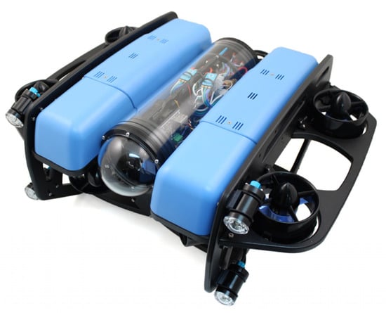
Figure 3.
Real shape of an ROV.
The ROV’s orientation followed the standard right-hand coordinate system (Figure 2). Thrusters were symmetrically distributed on the ROV frame to enable overactuated motion in all six degrees of freedom. This layout allowed full control of the surge, sway, heave, roll, pitch, and yaw and facilitated realistic control and response testing under multi-directional flow conditions.
Based on the theory above, we added three-dimensional ocean currents to the system.
2.2. Method Analyses
Before starting the simulation, we must determine the ROV’s path. As Figure 4 shows, its path was as follows.
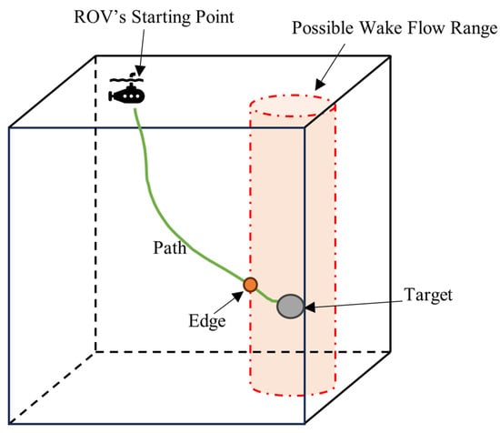
Figure 4.
The path that the ROV travels.
According to experimental observations, we defined d as the distance between the ROV and the target. When d was less than 4 m, the influence of the ocean wake flow should be taken into account in some cases. Figure 5 illustrates a typical wake flow pattern encountered as the ROV approached the target.
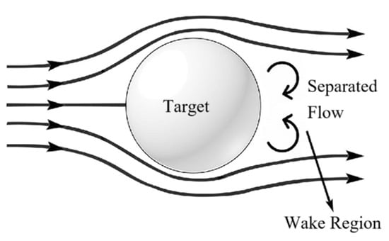
Figure 5.
A Typical type of wake flow.
As shown in Figure 5, the influence of wake flow varied significantly, depending on the ROV’s relative approach direction to the target. When the ROV approached the target head-on (i.e., directly facing the current), the impact of wake flow was minimal and could often be neglected. In contrast, wake-induced disturbances became more prominent when the ROV approached from the side or the rear, either perpendicular to the flow or aligned, and they must be considered in the trajectory and control model because wake turbulence introduces unpredictable velocity fluctuations and pressure gradients, which can degrade control accuracy and cause trajectory deviation, especially when using PID-based or linear control strategies. Therefore, we divided the directions from which the ROV approached the target into three parts, as shown in Figure 6.
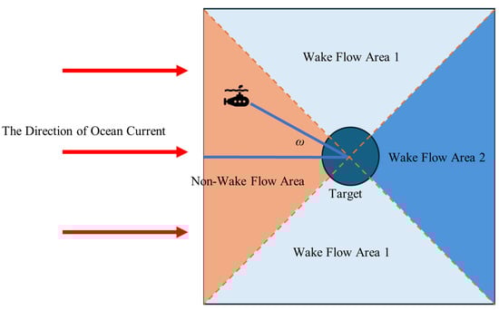
Figure 6.
Illustration of wake flow near the target, segmented into three analytical regions.
In the non-wake flow area, we only simulated the path under the influence of ocean currents, while in the wake flow area, both ocean currents and wake flow needed to be considered [19]. Based on Figure 6, in wake flow area 1, we considered the wake flow in the same direction as ocean currents, but in wake flow area 2, it was in the opposite direction.
ω denotes the angle between the ROV’s approach direction and the ocean current (as shown in Figure 6). The flow field around the target was divided into three regions based on ω:
- The non-wake flow area corresponded to ω ∈ [−45°, +45°], where the ROV approached from the front without entering the wake region;
- Wake flow area 1 covered the angular range ω ∈ (45°, 135°) ∪ (225°, −45°), where the ROV encountered lateral wake effects;
Wake flow area 2 was defined for ω ∈ [135°, 225], representing the direct downstream wake region behind the target.
According to DNV RP C205 [20], the velocity within the wake region vf can be estimated as a fraction of the freestream current velocity v. The wake deficit coefficient Δ, which depends on the geometry and blockage of the upstream obstacle, was used to characterize the velocity reduction inside the wake region. The relationship is typically expressed as follows:
vf = v (1 − Δ),
Thus, the wake velocity generally ranged from 30% to 80% of the freestream current velocity, consistent with engineering approximations suggested in DNV RP C205 and supported by empirical studies, such as those by Vermeer et al. Δ was set to 0.5 in wake flow area 1 and 0.3 in wake flow area 2.
This region-based classification is informed by classical wake flow theory and offers clear physical interpretability and engineering practicality. Compared to continuous gradient models, discrete disturbances improve simulation stability while sufficiently capturing the dominant characteristics of the flow field, making it suitable for path planning and control algorithm development [21]. According to the standard DNV RP C205, when detailed field measurements are not available, the variation in shallow tidal current velocity with depth may be modeled as a simple power law. Assuming unidirectional current, some parameters are defined as follows:
vc is the ocean current velocity at depth h;
v is the tidal current velocity at the still water level, which must be measured in the actual experiment;
z is the vertical distance from the still water level (positive upwards, typically negative);
h is the total water depth measured downward from the still water level.
α is an exponent, and typically, α = 1/7; we can calculate the speed of the ocean current:
To improve simulation efficiency while maintaining modeling accuracy, the tidal current velocity profile was simplified based on the operational depth range of the robot (0–25 m below the still water level). According to Equation (9), the velocity variation within this depth range was moderate and allowed for approximation. For example, assuming a total water depth d = 100 m, the distance from the still water level z = −60, and an empirical exponent α = 1/7, the velocity decreased gradually from the surface downward. The velocity was approximated to be vc = 0.14 × v. These representative values were derived from the theoretical profile and effectively reduced computational costs while preserving the fidelity required for motion simulation. The corresponding value was selected based on the robot’s real-time depth in actual implementation.
2.3. Building the Ocean Current Disturbance Module
To better illustrate the ocean currents, we decomposed the three-dimensional model, as shown in Figure 7.
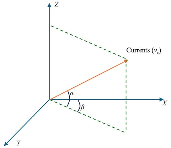
Figure 7.
Ocean current example model.
Based on Figure 7, if the angle between the current and the XOY plane was defined as φ, the angle between the current and the ZOX plane was θ, and the speed of the ocean current was vc. According to the knowledge of trigonometric functions, we can obtain the formula for calculating the components of the ocean current in all directions as follows:
Wake flow happened in the horizontal direction, making it easier to analyze. Figure 8 shows the decomposed wake flow model.
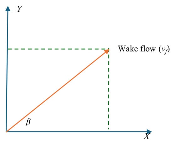
Figure 8.
Wake flow example model.
Using the same method as in Equation (10), we can obtain the formula for calculating the components of the wake flow in all directions as follows:
Thus, based on Figure 8 and Equations (8)–(11), we can calculate the influence of ocean currents and wake flow (vf) as follows:
- Non-wake flow area: V = Vcurrent;
- Wake flow area 1: V = Vcurrent + Vwake, that is:
- Wake flow area 2: V = Vcurrent − Vwake, which means:
The ROV’s approach direction relative to the ocean current was determined based on the initial and target positions, as illustrated in Figure 4. The approach angle ω, defined in Figure 6, was used to classify the flow interaction region and to select the appropriate control model accordingly:
- Non-wake flow area (ω ∈ [−45°, +45°]): When the ROV moved approximately in the same direction as the ocean current, approaching from the front without entering the wake region, Equation (11) was applied;
- Wake flow area 1: (ω ∈ (45°, 135°) ∪ (−135°, −45°)): When the ROV experienced lateral wake interference due to side-on current interaction, Equation (13) was used;
- Wake flow area 2: (ω ∈ [135°, 225°]): When the ROV moved directly against the current, entering the downstream wake region behind the target, Equation (14) was employed.
This classification balanced hydrodynamic realism with computational simplicity by adapting the model to varying current interaction scenarios.
According to the previous analysis, to incorporate the influence of ocean currents on the underwater robot’s trajectory, we only needed to modify the relative velocity components in the drag matrix’s X, Y, and Z directions (shown in Figure 2). Specifically, the relative velocity was defined as the difference between the vehicle’s body-fixed velocity and the ocean current velocity projected into the same frame. This approach followed the conventional assumption in underwater vehicle hydrodynamic modeling that the ocean current affects the system linearly by modifying the relative velocity vector, without introducing additional nonlinear terms [22,23]. Thus, the nonlinear terms in the dynamic model remained unchanged. The updated relative velocity vector was then used to calculate hydrodynamic damping forces, and the modified drag matrix [24] was expressed as:
By combining Equations (11), (13), and (14), we updated the components Du, Dv, and Dw in the drag matrix to Du1, Dv1, and Dw1, as follows:
Thus, the continuous influence of ocean currents on the underwater robot was successfully integrated into the simulation system.
3. Experimental Materials
Simulation Environment: All simulations were conducted using MATLAB R2022b and Simulink, developed by MathWorks Inc. This environment provided an integrated platform for modeling dynamic systems and performing time-domain simulations.
The hardware platform used for simulation was a ROG Gunship 6p laptop equipped with an NVIDIA RTX 3070 Ti GPU. The specific configuration included an Intel Core i9 processor and 32 GB of RAM. This setup ensured sufficient computational capability for real-time rendering and large matrix calculations, especially in simulating the six-degrees-of-freedom (6-DOF) dynamics of the ROV under complex ocean flow fields.
4. Experimental Results
The ROV’s trajectory was simulated in Simulink under the influence of ocean currents and wake flows. We could accurately simulate the ROV’s path in various scenarios by analyzing the wake flow from different directions and assessing its impact on the ROV’s motion. The simulation explored multiple orientations the ROV may face, allowing us to observe the resulting changes in its trajectory. The results were as follows: we determined that the range of wake flow was R = 2 m, the ocean current on the surface was v = 2 m/s, and the depth of the ocean was 100 m.
4.1. When the ROV Is Facing Directly Toward the Current
In this scenario, the ROV was oriented directly against the direction of the ocean current, resulting in minimal disturbance from wake flow. The simulation was configured with consistent parameters for the first and second path segments. Specifically, the ROV started at position [0, 0, −40] and aimed to reach the target location [−15, −15, −60]. The yaw angle at the target was set to 0°, while the ROV’s initial yaw was 165°, causing it to face nearly opposite the current.
βc = π/4, representing the current’s direction in the horizontal xy-plane, was measured counterclockwise from the x-axis, and
αc ≈ 0.955 rad, representing the elevation angle of the current from the xy-plane toward the z-axis.
This configuration ensured that the current vector was oriented near the target direction, resulting in an angular separation of approximately 180° between the current and the desired trajectory. The resulting ROV trajectory under these conditions is illustrated [25] in Figure 9.
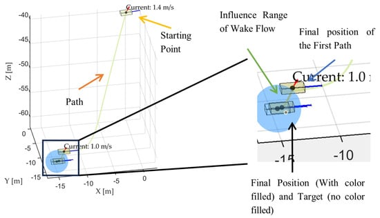
Figure 9.
When the ROV moves facing the ocean current.
In this sample, the ROV started at [0, 0, −40] and finally reached [−14.8114, −14.5905, −60.039]. Using the Euclidean distance formula, there was approximately 0.4525 m between the final position and the target. The component-wise deviations were 0.1886 m in the x-direction, 0.4095 m in the y-direction, and 0.0390 m in the z-direction.
4.2. When the ROV Is Side-On to the Current
In this scenario, the ROV moved along the direction [−15, −15, −60], while the ocean current flowed orthogonally to its trajectory. To achieve a 90° angle between the current and the path, the current vector was defined as [1, −1, 0], lying purely in the horizontal plane. This corresponded to an azimuth angle βc = −π/4 and elevation angle αc = π/2.
With the ROV’s initial position at [0, 0, −40], target at [−15, −15, −60], and target yaw set to 0°, this setup allowed us to analyze how lateral wake effects influenced the vehicle. The simulation outcome under this perpendicular interaction is visualized in Figure 10.
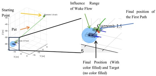
Figure 10.
When the ROV moves side-on to the ocean current.
In this sample, the ROV started at [0, 0, −40] and finally reached [−14.6195, −14.4217, −60.0334]. The resulting Euclidean distance between the two points was approximately 0.8221 m. The individual absolute deviations were 0.3805 m in the x-direction, 0.5783 m in the y-direction, and 0.0334 m in the z-direction.
4.3. The ROV Is Facing Away from the Current
In this scenario, the ROV moved along the vector direction [−15, −15, −60] while the ocean current flowed orthogonally to its trajectory. To establish a 0° angle between the current and the ROV’s path, the current vector was defined as [1, −1, 0], which lay entirely within the horizontal xy-plane. This configuration corresponded to an azimuth angle βc = −3π/4 and an elevation angle αc ≈ 2.34 rad, representing a purely horizontal flow with no vertical component.
The ROV started from the initial position [0, 0, −40] and navigated toward the target position [−15, −15, −60], with the target yaw set to 0°. This setup facilitated the investigation of how lateral ocean currents and resulting wake flow influenced the vehicle’s maneuvering and trajectory correction. The simulation results for this perpendicular interaction are presented in Figure 11.
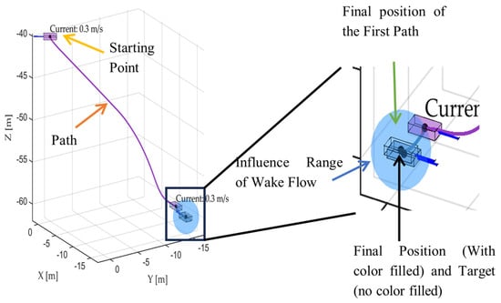
Figure 11.
When the ROV moves facing away from the current.
In this sample, the ROV started at [0, 0, −40] and finally reached [−14.9869, −14.7836, −60.148]. The resulting Euclidean distance between the two points was approximately 0.6924 m. The absolute deviations in each direction were 0.3805 m along the x-axis, 0.5783 m along the y-axis, and 0.0334 m along the z-axis.
Table 1 compares three scenarios of the ROV approach relative to the ocean current. The ROV exhibited the highest efficiency when aligned with the current, achieving the target with minimal deviation. In contrast, lateral approaches resulted in moderate sideways drift, while moving against the current demanded substantial corrective actions and caused trajectory delays. These findings highlight the critical role of orientation in path planning within dynamic underwater environments.

Table 1.
The results of three cases.
Such insights are valuable for developing adaptive control strategies for ROVs operating under varying flow conditions, ensuring robust performance despite changing current directions [26,27].
5. Comparison Between the Proposed Model and Current Mainstream Models
This model was based on the existing six-degrees-of-freedom ROV model, with optimizations made to the resistance matrix and including the three-dimensional ocean current interference on the underwater robot’s motion path. Additionally, the plotting functions of the original model were modified to enable the simulation of the underwater robot’s three-dimensional path.
To objectively highlight the advantages and innovations of the proposed model, a comparative simulation was conducted against a baseline model. To emphasize the differences in behavior under dynamic flow conditions, we intentionally used an intensified ocean current velocity of v = 7 m/s, not to represent typical marine conditions but to amplify the response characteristics of the models for clearer observation. In this scenario, the ROV started from position [0, 0, −40] and aimed for a target at [−15, −15, −60]. The water depth was set to 30 m, with the ROV initially located 12 m below the still water level. The baseline model results are presented in Figure 12, while the simulation outputs from the proposed model are shown in Figure 9, Figure 10 and Figure 11.
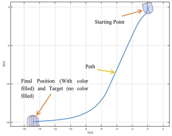
Figure 12.
The simulation result of the previous model.
The results were as follows: In the previous model, the ROV finally reached [−14.96, −14.77, −60.34], which was considered to have no ocean currents and wake flow because it reached the target with minor inaccuracy, which is not based on real-life. Compared with Figure 13, where a considerable gap was found between the target and final positions, the ocean current successfully influenced the path of the ROV. Thus, the proposed model successfully figured out how ocean currents influenced the path of an ROV’s track with a 3D visualization.
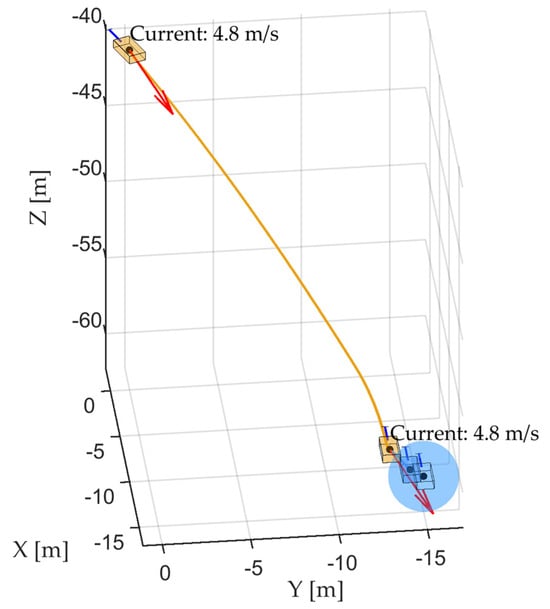
Figure 13.
The simulation result of the proposed model.
6. Discussion and Future Work
This study investigated the motion behavior of an ROV under the influence of ocean currents and wake disturbances. The primary contribution lay in improving the accuracy of the hydrodynamic damping matrix D, which is often oversimplified in traditional models. Refining this matrix based on empirical data and theoretical corrections, we aimed to enhance the ROV’s responsiveness to lateral and angular hydrodynamic forces.
However, several simplifications in the overall system remain, mainly inherited from the baseline control framework and the need to constrain computational complexity. These include the following:
- (1)
- The control structure is based on a traditional PID controller, which, although widely used in marine systems, does not adapt to environmental variations or uncertainties.
- (2)
- The environmental model assumes quasi-steady ocean currents and simplified wake interference, which may not fully capture real-world turbulence or chaotic fluctuations.
- (3)
- The simulation does not incorporate external feedback loops, real-time sensor data, or actuator dynamics.
- (4)
- The study is limited to a single-ROV scenario and does not account for distributed cooperation or inter-ROV interference.
While these simplifications are standard in preliminary marine vehicle modeling, we performed a comparative simulation to evaluate their quantitative impact. Specifically, we examined the difference in trajectory when wake flow effects were excluded from the damping matrix D. The results indicate that neglecting wake interference can result in trajectory deviations of up to 3.9% in lateral motion under certain ocean current configurations. Therefore, the assumption of steady-state flow and uniform damping, as used in traditional models, may underestimate hydrodynamic disturbances in real-world conditions. This further justifies the inclusion of an empirically corrected damping matrix in our study. Based on similar findings in related hydrodynamic simulation studies, other assumptions, such as fluid incompressibility and rigid body modeling, are expected to introduce smaller errors (typically below 1.5%) in low-speed operations.
Moreover, the current damping model assumes a diagonal damping matrix with simplified quadratic nonlinear terms, neglecting cross-coupling between different degrees of freedom and potential higher-order nonlinear damping effects. While this assumption balances model complexity and computational efficiency, it limits the ability to capture complex hydrodynamic interactions that may significantly influence ROV dynamics in turbulent or rapidly changing flow conditions. Future research will focus on incorporating these effects to enhance model fidelity and simulation accuracy.
While unnecessary for focusing on the damping model’s impact, these constraints could reduce the model’s fidelity when applied to field deployments or more complex operational conditions. As noted by the reviewers, unexpected environmental fluctuations, model uncertainties, and control delays may affect both performance and stability, especially in unstructured or chaotic marine environments.
In future works, we plan to address these limitations in several directions. First, we will consider time-varying and turbulent flow fields to better model realistic ocean disturbances. Second, advanced control strategies, such as model-predictive control (MPC) or data-driven adaptive methods, may be incorporated to improve system robustness. Third, extending the framework to include multi-ROV interactions and cooperative decision-making will allow for more complex mission scenarios. Additionally, improving the visual simulation platform and analyzing computational efficiency will be necessary for real-time deployment on embedded hardware.
This work provides a solid foundation for these enhancements by addressing a key physical component—the damping matrix—while outlining the path toward more comprehensive and field-ready ROV navigation systems.
7. Conclusions
This study addresses the issue that existing simulation systems overlook or only simulate the impact of two-dimensional ocean currents on ROV motion trajectories [28]. It also acknowledges that these systems’ visualization of simulation results could be improved. Focusing on the ROV, a highly modular simulation system was built using MATLAB and Simulink to optimize these issues. The system primarily optimized the resistance matrix in the original simulation model, decomposing three-dimensional ocean currents into the X, Y, and Z directions. Simulations were performed on the relative velocity in each direction, enabling the simulation of ROV motion trajectories under ocean current interference. Additionally, to provide an intuitive display of simulation results and data, the model incorporated a 3D plotting module, allowing users to rotate the 3D view and observe the results.
In contrast to traditional path planning simulations that often ignore the impact of current direction and magnitude, this study incorporated a complete 3D current model to replicate realistic underwater conditions better, which enhanced the validity of the simulation outcomes and provided a more comprehensive understanding of ROV trajectory behavior under various current alignments. Yaw dynamics and directional drift also improved upon prior simplified methods, making the results more applicable to real-world operations.
Although this research has made some progress, many areas still warrant further exploration. Future studies may incorporate time-varying or turbulent currents and autonomous decision-making for real-time path correction. Additionally, game theory or distributed control methods could be introduced to extend the control of a single ROV to collaborative control and path planning for multiple ROVs. Artificial intelligence (AI) technologies, such as deep learning algorithms, could be integrated on the technical application front. Combined with deploying distributed sensor networks and a hardware/software simulation test platform, this could push advancements in the direction of intelligence and multi-functionality.
Author Contributions
Conceptualization, Y.Z. and S.X.; Methodology, Y.Z.; Software, Y.Z.; Validation, S.X.; Investigation, B.X.; Resources, L.L.; Writing—original draft, Y.Z. and S.X.; Writing—review & editing, S.X. and X.Z.; Supervision, X.Z. and C.X.; Project administration, C.X. All authors have read and agreed to the published version of the manuscript.
Funding
This work was supported in part by the Guangdong Ocean University Research Project Initiation Fund (360302042202) and the China National College Students Innovation and Entrepreneurship Training Program Funding Project (202410566040).
Data Availability Statement
There were no new data created, and there were no particular data used during the research.
Conflicts of Interest
The authors declare no conflicts of interest. The funders had no role in the design of the study; in the collection, analyses, or interpretation of data; in the writing of the manuscript; or in the decision to publish the results.
References
- Amundsen, H.B.; Caharija, W.; Pettersen, K.Y. Autonomous ROV Inspections of Aquaculture Net Pens Using DVL. IEEE J. Ocean. Eng. 2022, 47, 1–19. [Google Scholar] [CrossRef]
- Bartlett, B.; Trslic, P.; Santos, M.; Penica, M.; Riordan, J.; Dooly, G. Dynamic Positioning System for low-cost ROV. In Proceedings of the OCEANS 2023—Limerick, Limerick, Ireland, 5–8 June 2023; pp. 1–5. [Google Scholar]
- Zhao, J.; Xu, Y.; Lei, L. Establishment of a simulator for intelligent path planning of underwater robots. J. Syst. Simul. 2004, 11, 2448–2450. [Google Scholar]
- Xu, L.; Bian, Y.; Zong, G. Path Control and Simulation of Underwater Robots. J. Beihang Univ. 2005, 2, 162–166. [Google Scholar]
- Ren, C.; Wan, N.; Wang, S.; Wang, D. Research on Optimal Path Planning Problem for Autonomous Underwater Robots. China Navig. 2003, 9, 14–18. [Google Scholar]
- Li, Y.; He, J.; Jiang, Y.; An, L. Semi physical simulation of AUV return and seated docking. Robotics 2017, 39, 119–128. [Google Scholar]
- Gabl, R.; Davey, T.; Cao, Y.; Li, Q.; Li, B.; Walker, K.L.; Giorgio-Serchi, F.; Aracri, S.; Kiprakis, A.; Stokes, A.A.; et al. Hydrodynamic loads on a restrained ROV under waves and current. Ocean. Eng. 2021, 234, 109279. [Google Scholar] [CrossRef]
- Rostamzadeh-Renani, M.; Rostamzadeh-Renani, R.; Baghoolizadeh, M.; Azarkhavarani, N.K. The effect of vortex generators on the hydrodynamic performance of a submarine at a high angle of attack using a multi-objective optimization and computational fluid dynamics. Ocean. Eng. 2023, 282, 114932. [Google Scholar] [CrossRef]
- Rostamzadeh-Renani, M.; Baghoolizadeh, M.; Sajadi, S.M.; Rostamzadeh-Renani, R.; Azarkhavarani, N.K.; Salahshour, S.; Toghraie, D. A multi-objective and CFD based optimization of roof-flap geometry and position for simultaneous drag and lift reduction. Propuls. Power Res. 2024, 13, 26–45. [Google Scholar] [CrossRef]
- Liu, P.; Tian, L.; Qiu, T.; Li, L.; Huang, F.; Yin, B.; Zhu, G. Optimization simulation of ROV controller parameters based on combinatorial optimization algorithm. Mar. Eng. Equip. Technol. 2023, 10, 64–70. [Google Scholar]
- Long, C.; Qin, X.; Bian, Y.; Xu, B.; Hu, M. Trajectory tracking control of an ROV using model predictive control considering external disturbances. In Proceedings of the 2021 5th CAA International Conference on Vehicular Control and Intelligence (CVCI), Tianjin, China, 29–31 October 2021; pp. 1–5. [Google Scholar]
- Lack, S.; Rentzow, E.; Jeinsch, T. Trajectory generation for a quaternion based 6-DoF ROV tracking controller. In Proceedings of the 2022 30th Mediterranean Conference on Control and Automation (MED), Vouliagmeni, Greece, 28 June–1 July 2022; pp. 414–419. [Google Scholar]
- Daddi, A.S.; Gundewar, P.P.; Mulay, G. MIMO Model Development of the Navigational System of an Underwater ROV. In Proceedings of the 2022 International Conference for Advancement in Technology (ICONAT), Goa, India, 21–22 January 2022; pp. 1–7. [Google Scholar]
- Huang, H.; Wan, L.; Pang, Y.; Qin, Z.; Zeng, W. Research on fault-tolerant control of SY-II remote-controlled underwater robot thruster. J. Appl. Basic Eng. Sci. 2012, 20, 1118–1128. [Google Scholar]
- Mulero-Martínez, J.I. A new factorization of the Coriolis/centripetal matrix. Robotica 2009, 27, 689–700. [Google Scholar] [CrossRef]
- Fossen, T.I. Fossen’s Marine Craft Model. Wikipedia. 2002. Available online: https://www.fossen.biz/html/marineCraftModel.html (accessed on 27 February 2025).
- Fossen, T.I. Handbook of Marine Craft Hydrodynamics and Motion Control; Wiley: Hoboken, NJ, USA, 2011. [Google Scholar]
- Hosseinnajad, A.; Loueipour, M. Design of a Robust Observer-based DP Control System for an ROV with Unknown Dynamics Including Thruster Allocation. In Proceedings of the 2021 7th International Conference on Control, Instrumentation and Automation (ICCIA), Tabriz, Iran, 23–24 February 2021; pp. 1–6. [Google Scholar]
- Zhao, M.; Chen, Y.; Jiang, J. Hydrodynamics and Wake Flow Analysis of a Floating Twin-Rotor Horizontal Axis Tidal Current Turbine in Roll Motion. J. Mar. Sci. Eng. 2023, 11, 1615. [Google Scholar] [CrossRef]
- Det Norske Veritas. DNV-RP-C205: Environmental Conditions and Environmental Loads; DNV: Høvik, Norway, 2010. [Google Scholar]
- Brandt, A.; Sebben, S.; Jacobson, B. Base wake dynamics and its influence on driving stability of passenger vehicles in crosswind. J. Wind. Eng. Ind. Aerodyn. 2022, 230, 105164. [Google Scholar] [CrossRef]
- Fossen, T.I. Guidance and Control of Ocean Vehicles; John Wiley & Sons: Chichester, UK, 1994. [Google Scholar]
- Prestero, T. Verification of a Six-Degree of Freedom Simulation Model for the REMUS Autonomous Underwater Vehicle; MIT/WHOI Joint Program: Cambridge, MA, USA, 2001. [Google Scholar]
- Sun, G.; Su, Y.; Mao, Y.; Xie, J.; Jiao, H.; Qv, J. Multi level thrust allocation strategy for hybrid propulsion ROV based on fuzzy logic. Robot 2023, 45, 472–482. [Google Scholar]
- Liu, S.; Deng, Z.; Sun, J.; Ding, L. Introduction to the Drawing Function of MATLAB Software. Comput. Learn. 2000, 3, 49. [Google Scholar]
- Zou, Y.; Tao, Z.; Li, X. Research on Attitude Control of Underwater Robots Based on Active Disturbance Rejection Controller. Chem. Autom. Instrum. 2024, 51, 621–630. [Google Scholar]
- Xue, Y.; Wang, S.; Ma, W.; Zeng, Z. Underwater Wall-Climbing Inspection ROV Scheme Design and Flow Resistance Simulation Based on BlueROV2 Modification. In Proceedings of the 2023 IEEE 3rd International Conference on Software Engineering and Artificial Intelligence (SEAI), Xiamen, China, 16–18 June 2023; pp. 215–219. [Google Scholar]
- Yao, X.L.; Wang, F.; Wang, J.F.; Wang, X. A method for optimal energy consumption path planning of AUV under time-varying ocean flow field. Control Decis. 2020, 35, 2424–2432. [Google Scholar]
Disclaimer/Publisher’s Note: The statements, opinions and data contained in all publications are solely those of the individual author(s) and contributor(s) and not of MDPI and/or the editor(s). MDPI and/or the editor(s) disclaim responsibility for any injury to people or property resulting from any ideas, methods, instructions or products referred to in the content. |
© 2025 by the authors. Published by MDPI on behalf of the International Institute of Knowledge Innovation and Invention. Licensee MDPI, Basel, Switzerland. This article is an open access article distributed under the terms and conditions of the Creative Commons Attribution (CC BY) license (https://creativecommons.org/licenses/by/4.0/).