
Enhanced Grey Wolf Optimization for Efficient Transmission Power Optimization in Wireless Sensor Network


Abstract
1. Introduction
2. Methodology
2.1. WSN Transmission Power
2.2. Optimization Algorithms
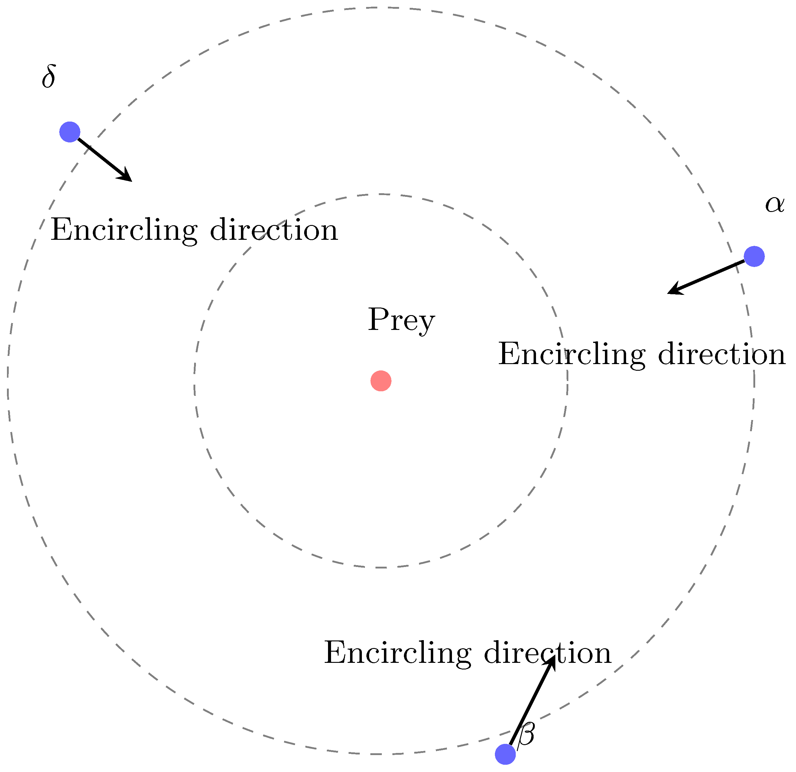
2.2.1. Grey Wolf Optimizer
- Alpha (): The best solution, leading the search.
- Beta (): The second-best solution, assisting in leadership.
- Delta (): The third-best solution, subordinate to and .
- Omega (): The remaining wolves, following , , and .
Encircling Prey
Proposed Enhanced GWO with Non-Linear Decreasing Coefficient
- Problem dimensionality (D): 30;
- Number of wolves (N): 30;
- Maximum iterations (T): 100;
- Number of independent runs: 30.
Hunting Behavior
Convergence and Termination
Application in WSNs
- Energy Efficiency: Minimizing energy consumption by optimizing cluster head selection and communication paths.
- Delay Reduction: Reducing end-to-end latency for time-sensitive IoT applications.
- Network Throughput: Enhancing packet delivery ratio and overall network performance.
- E: Total energy consumption;
- D: Average delay in data transmission;
- T: Total network throughput;
- : Weighting factors balancing the objectives.
2.2.2. Particle Swarm Optimization
- : velocity of particle i at iteration t;
- : position of particle i at iteration t;
- : personal best position of particle i;
- : global best position in the swarm;
- w: inertia weight, controlling the balance between exploration and exploitation;
- : cognitive and social coefficients, respectively;
- : random numbers uniformly distributed in .
2.2.3. Bi-Directional Evolutionary Structural Optimization
Mathematical Formulation
- 1.
- Objective Function: The objective function for minimizing compliance is defined aswhere
- C: Structural compliance;
- : Global displacement vector;
- : Global stiffness matrix.
- 2.
- Volume Constraint: The optimization problem must satisfy a volume constraint:where
- V: Total material volume;
- : Maximum allowable material volume;
- : Total number of finite elements;
- : Volume of element e.
- 3.
- Sensitivity Analysis: The sensitivity of the objective function with respect to the design variable is calculated aswhere and are the displacement vector and stiffness matrix of element e, respectively.
Convergence and Termination
- 4.
- Evolutionary Update Rule: The material distribution is updated iteratively usingwhere is a threshold determined by the volume constraint and evolutionary ratio.
- 5.
- Bi-directional Adjustment: BESO allows both the addition and removal of materials, enabling a balanced search for optimal topology:where is the material adjustment increment.
Application in Multi-Scale Optimization
- : Compliance of the structure;
- : Penalization term for multi-scale connectivity;
- : Weighting factors balancing the objectives.
Performance in Structural Design
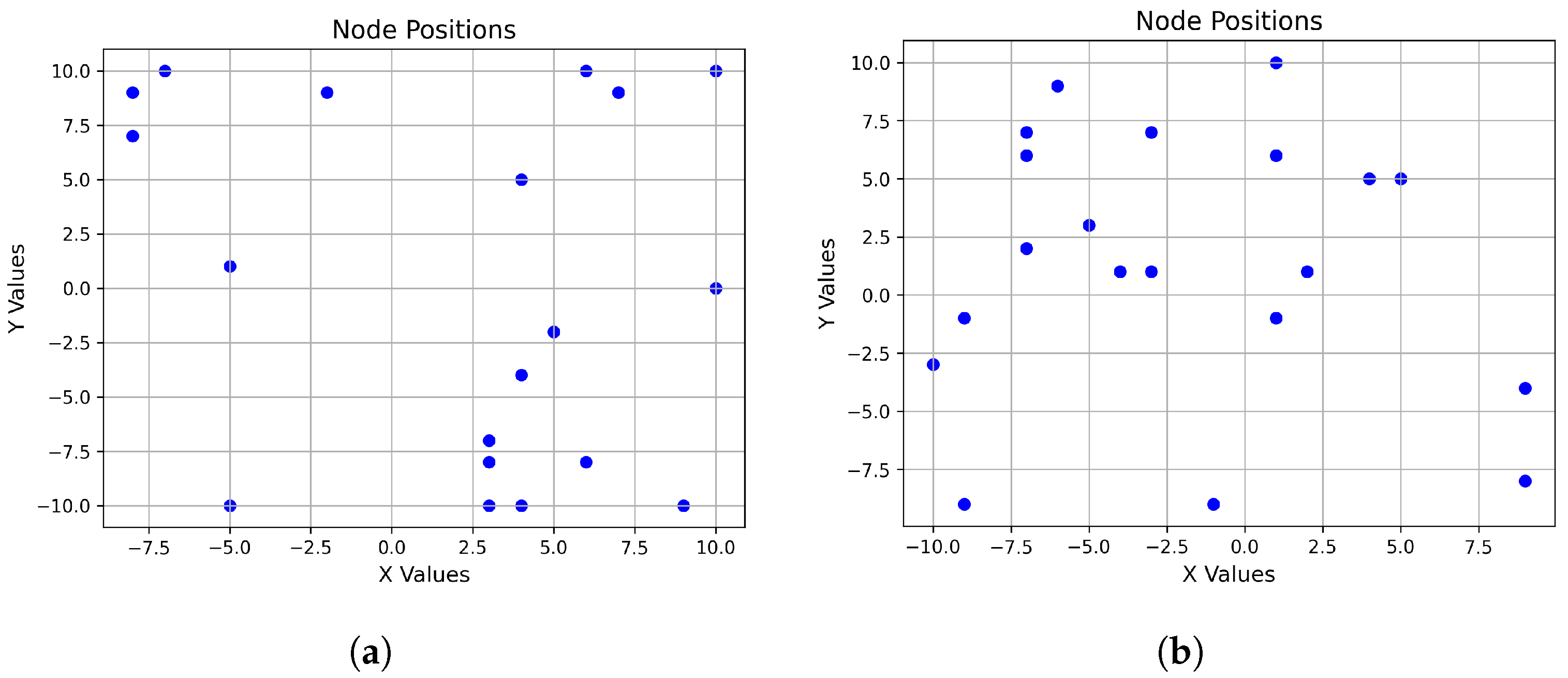
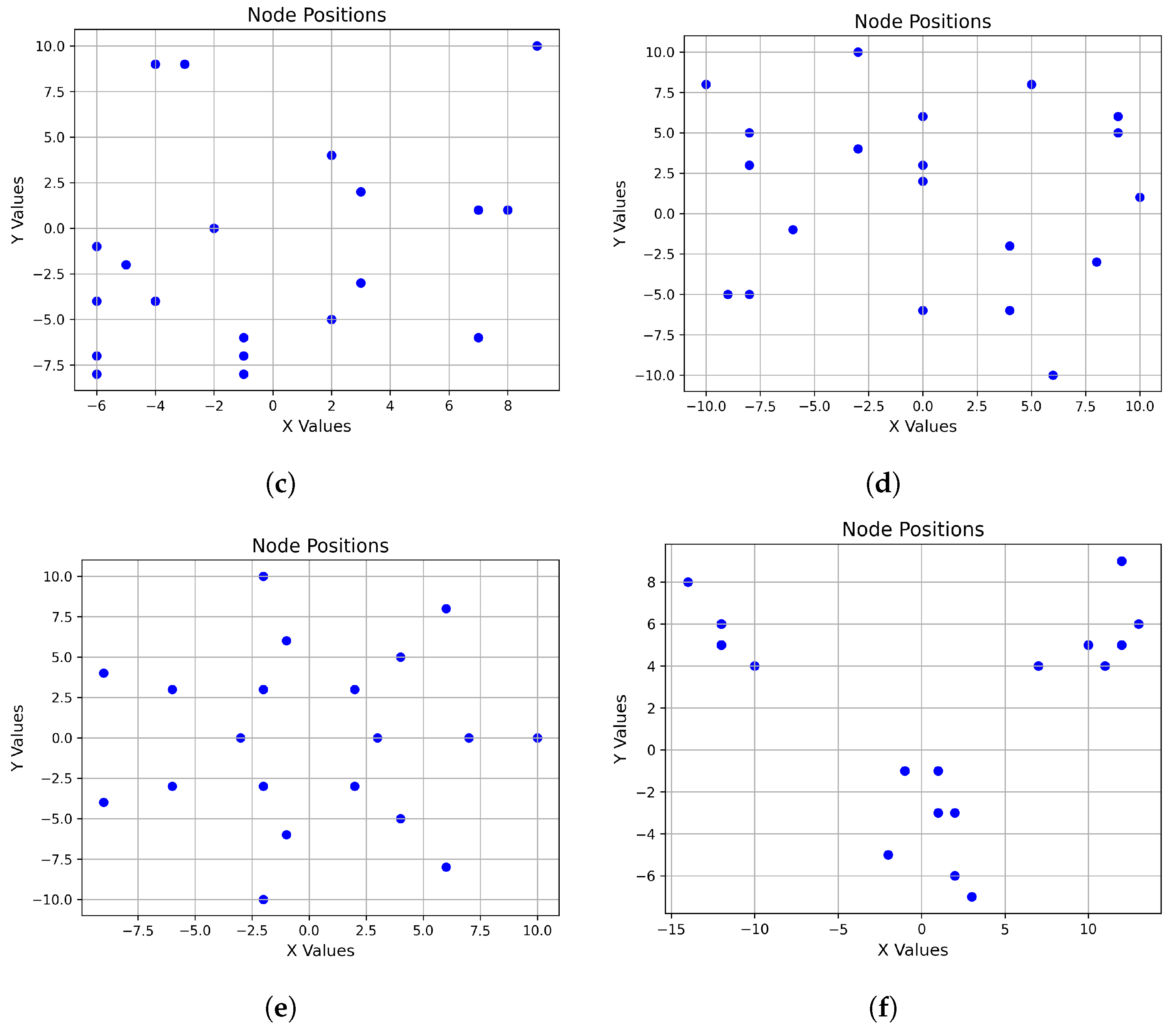
2.3. Experimental Scenario
3. Results and Discussion

| Algorithm | Minimum | Maximum | Mean |
|---|---|---|---|
| BESO | 10.429456 | 20.312532 | 14.171138 |
| PSO | 11.898477 | 33.346832 | 18.473567 |
| GWO | 13.291528 | 21.313970 | 16.461065 |
| EGWO | 13.619340 | 21.6570003 | 19.445919 |
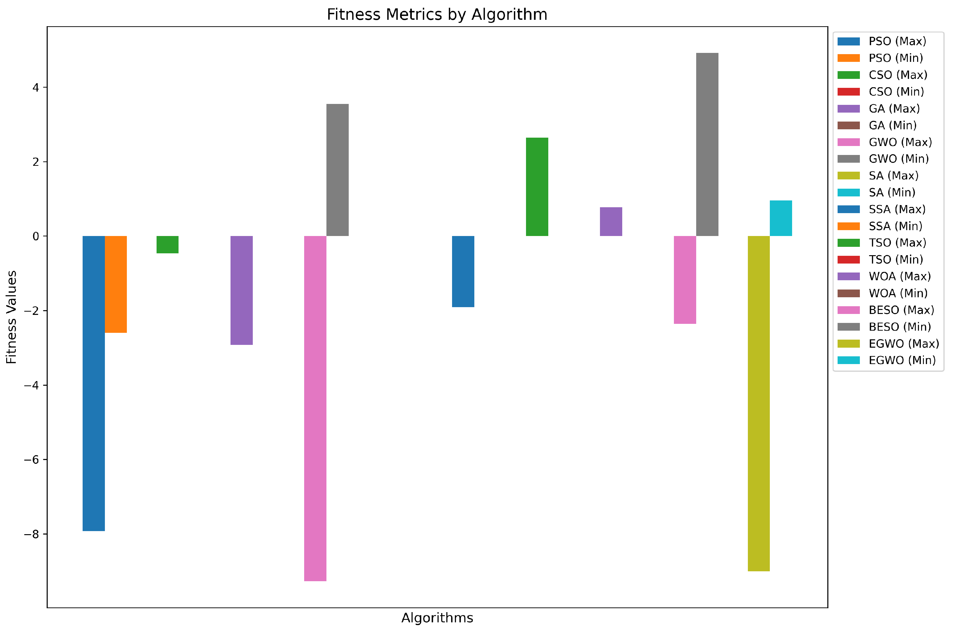
| Algorithm | Minimum | Maximum | Mean |
|---|---|---|---|
| BESO | −2.357431 | 4.919863 | 2.214195 |
| PSO | −7.926426 | −2.605397 | −3.725375 |
| GWO | −9.274447 | 3.547884 | −0.614383 |
| EGWO | −9.006406 | 0.953669 | −4.150733 |
4. Conclusions
Author Contributions
Funding
Data Availability Statement
Acknowledgments
Conflicts of Interest
References
- Precedence Research. Wireless Sensor Market Report 2024. Available online: https://www.precedenceresearch.com/wireless-sensor-market (accessed on 26 January 2025).
- GlobeNewswire. Industrial Wireless Sensor Network Global Market Report. 2023. Available online: https://www.globenewswire.com/news-release/2023/03/16/2628826/28124/en/Industrial-Wireless-Sensor-Network-Global-Market-Report-2023-Sector-to-Reach-16-1-Billion-by-2028-at-a-CAGR-of-18-21.html (accessed on 26 January 2025).
- Gupta, A.; Gulati, T.; Bindal, A.K. Wsn based iot applications: A review. In Proceedings of the 2022 10th International Conference on Emerging Trends in Engineering and Technology—Signal and Information Processing (ICETET-SIP-22), Nagpur, India, 29–30 April 2022; pp. 1–6. [Google Scholar] [CrossRef]
- Jamshed, M.A.; Ali, K.; Abbasi, Q.H.; Imran, M.A.; Ur-Rehman, M. Challenges, applications, and future of wireless sensors in internet of things: A review. IEEE Sens. J. 2022, 22, 5482–5494. [Google Scholar] [CrossRef]
- Neeha, S.; Charles, I.; Krishna, S.V.; Swarnakar, S. Performance analysis of leach, leach-c, ts-leach, mod-leach in wsn. Int. J. Comput. Intell. Commun. Technol. 2022, 11, 4–8. [Google Scholar] [CrossRef]
- Gupta, A.D.; Sathiyasekar, K.; Krishnamoorthy, R.; Arun, S.; Thiyagarajan, R.; Padmapriya, S. Proposed ga algorithm with h-heed protocol for network optimization using machine learning in wireless sensor networks. In Proceedings of the 2022 Second International Conference on Artificial Intelligence and Smart Energy (ICAIS), Coimbatore, India, 23–25 February 2022; pp. 1402–1408. [Google Scholar] [CrossRef]
- Ramadhan, F.; Munadi, R.; Istikmal. Modified combined leach and pegasis routing protocol for energy efficiency in iot network. In Proceedings of the 2021 IEEE International Seminar on Application for Technology of Information and Communication (iSemantic), Semarangin, Indonesia, 18–19 September 2021; pp. 389–394. [Google Scholar] [CrossRef]
- Redjimi, K.; Redjimi, M. The deec and edeec heterogeneous wsn routing protocols. Int. J. Adv. Netw. Appl. 2022, 13, 5045–5051. [Google Scholar] [CrossRef]
- Wodajo, H.H.; Kumar, K.S.A.; Kidane, G.T.; Hababa, S.M. Performance Evaluation of LEACH, PEGASIS and TEEN Routing Protocols in Wireless Sensor Networks Based on Network Lifetime. Int. J. Adv. Netw. Appl. 2021, 13, 4955–4961. [Google Scholar] [CrossRef]
- Sahoo, B.M.; Amgoth, T.; Pandey, H.M. Particle swarm optimization based energy efficient clustering and sink mobility in heterogeneous wireless sensor network. Ad Hoc Netw. 2020, 106, 102237. [Google Scholar] [CrossRef]
- Xiao, X.; Huang, H. A clustering routing algorithm based on improved ant colony optimization algorithms for underwater wireless sensor networks. Algorithms 2020, 13, 250. [Google Scholar] [CrossRef]
- Moshref, M.; Al-Sayyed, R.; Al-Sharaeh, S. An enhanced multi-objective non-dominated sorting genetic routing algorithm for improving the qos in wireless sensor networks. IEEE Access 2021, 9, 149176–149195. [Google Scholar] [CrossRef]
- Jacob, I.J.; Darney, P.E. Artificial bee colony optimization algorithm for enhancing routing in wireless networks. J. Artif. Intell. Capsul. Netw. 2021, 3, 62–71. [Google Scholar] [CrossRef]
- Barzin, A.; Sadegheih, A.; Zare, H.K.; Honarvar, M. A hybrid swarm intelligence algorithm for clustering-based routing in wireless sensor networks. J. Circuits Syst. Comput. 2020, 29, 2050163. [Google Scholar] [CrossRef]
- da Silva Fré, G.L.; de Carvalho Silva, J.; Reis, F.A.; Mendes, L.D.P. Mendes, Particle swarm optimization implementation for minimal transmission power providing a fully-connected cluster for the internet of things. In Proceedings of the 2015 International Workshop on Telecommunications (IWT), Santa Rita do Sapucai, Brazil, 14–17 June 2015; pp. 1–7. [Google Scholar] [CrossRef]
- ElMessmary, M.H.; Diab, H.Y.; Abdelsalam, M.; Moussa, M.F. A novel optimization algorithm inspired by Egyptian stray dogs for solving multi-objective optimal power flow problems. Appl. Syst. Innov. 2024, 7, 122. [Google Scholar] [CrossRef]
- Mirjalili, S.; Mirjalili, S.M.; Lewis, A. Grey Wolf Optimizer. Adv. Eng. Softw. 2014, 69, 46–61. [Google Scholar] [CrossRef]
- Jaiswal, K.; Anand, V. A grey-wolf based optimized clustering approach to improve qos in wireless sensor networks for iot applications. Peer-to-Peer Netw. Appl. 2021, 14, 1943–1962. [Google Scholar] [CrossRef]
- Mukherjee, A.; Goswami, P.; Yan, Z.; Yang, L.; Rodrigues, J.J.P.C. Adai and adaptive pso-based resource allocation for wireless sensor networks. IEEE Access 2019, 7, 131163–131171. [Google Scholar] [CrossRef]
- Kazakis, G.; Lagaros, N.D. Multi-scale concurrent topology optimization based on beso, implemented in matlab. Appl. Sci. 2023, 13, 10545. [Google Scholar] [CrossRef]
- Tang, M.; Xin, Y.; Qiao, Y. Multi-objective resource allocation algorithm for wireless sensor network based on improved simulated annealing. Adhoc Sens. Wirel. Netw. 2020, 47, 157–173. [Google Scholar]
- Brindha, S.; Bhargavi, K.V.; Kamali, T. Optimal cluster minimization for vanets using modified tuna swarm optimization. In Proceedings of the 2023 IEEE 7th International Conference on Trends in Electronics and Informatics (ICOEI), Tirunelveli, India, 11–13 April 2023; pp. 1389–1393. [Google Scholar] [CrossRef]
- Ajmi, N.; Helali, A.; Lorenz, P.; Mghaieth, R. Mwcsga—Multi weight chicken swarm based genetic algorithm for energy efficient clustered wireless sensor network. Sensors 2021, 21, 791. [Google Scholar] [CrossRef] [PubMed]
- Zishan, F.; Mansouri, S.; Abdollahpour, F.; Grisales-Noreña, L.F.; Montoya, O.D. Allocation of renewable energy resources in distribution systems while considering the uncertainty of wind and solar resources via the multi-objective salp swarm algorithm. Energies 2023, 16, 474. [Google Scholar] [CrossRef]
- Rana, N.; Jeribi, F.; Siddiqui, S.T. Efficient resource allocation in cloud data centers using the whale optimization algorithm with adaptive penalty function. In Proceedings of the 2023 IEEE International Conference on Networking, Sensing and Control (ICNSC), Marseille, France, 25–27 October 2023; pp. 1–7. [Google Scholar] [CrossRef]
- Nuha, H.; Liu, B.; Mohandes, M.; Balghonaim, A.; Fekri, F. Seismic data modeling and compression using particle swarm optimization. Arab. J. Geosci. 2021, 14, 2542. [Google Scholar] [CrossRef]
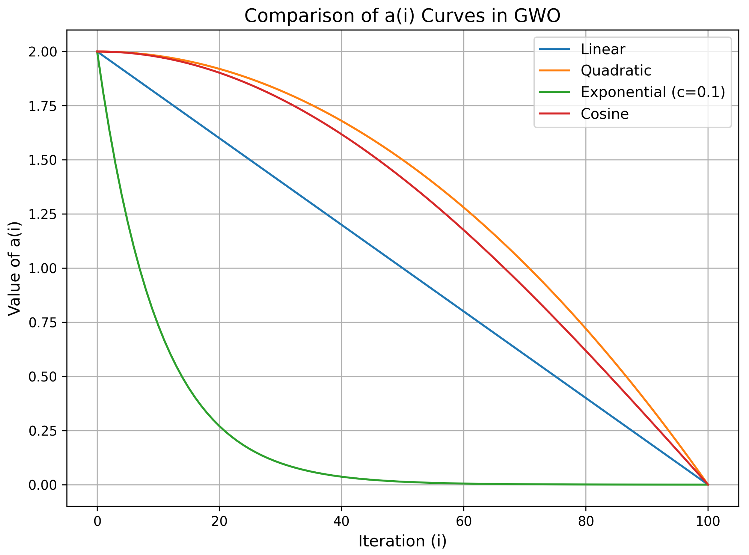
| Method | Mean Fitness | Std Dev Fitness | Avg. Convergence Iterations | Execution Time (s) |
|---|---|---|---|---|
| Linear | 40 | 0.045 | ||
| Quadratic | 38 | 0.048 | ||
| Exponential | 35 | 0.042 | ||
| Cosine | 48 | 0.050 |
| Parameter | Value [Unit] |
|---|---|
| Number of Sensor Nodes | 20 |
| Area for Random Sensors | |
| Distribution (L × L) | 20 [m] × 20 [m] |
| Sensor Transmission Frequency (f) | 915 [MHz] |
| Sensor Transmission Power Range | |
| (xMin; xMax) | (−30, 0) [dBm] |
| Sensor Sensitivity () | −60 [dBm] |
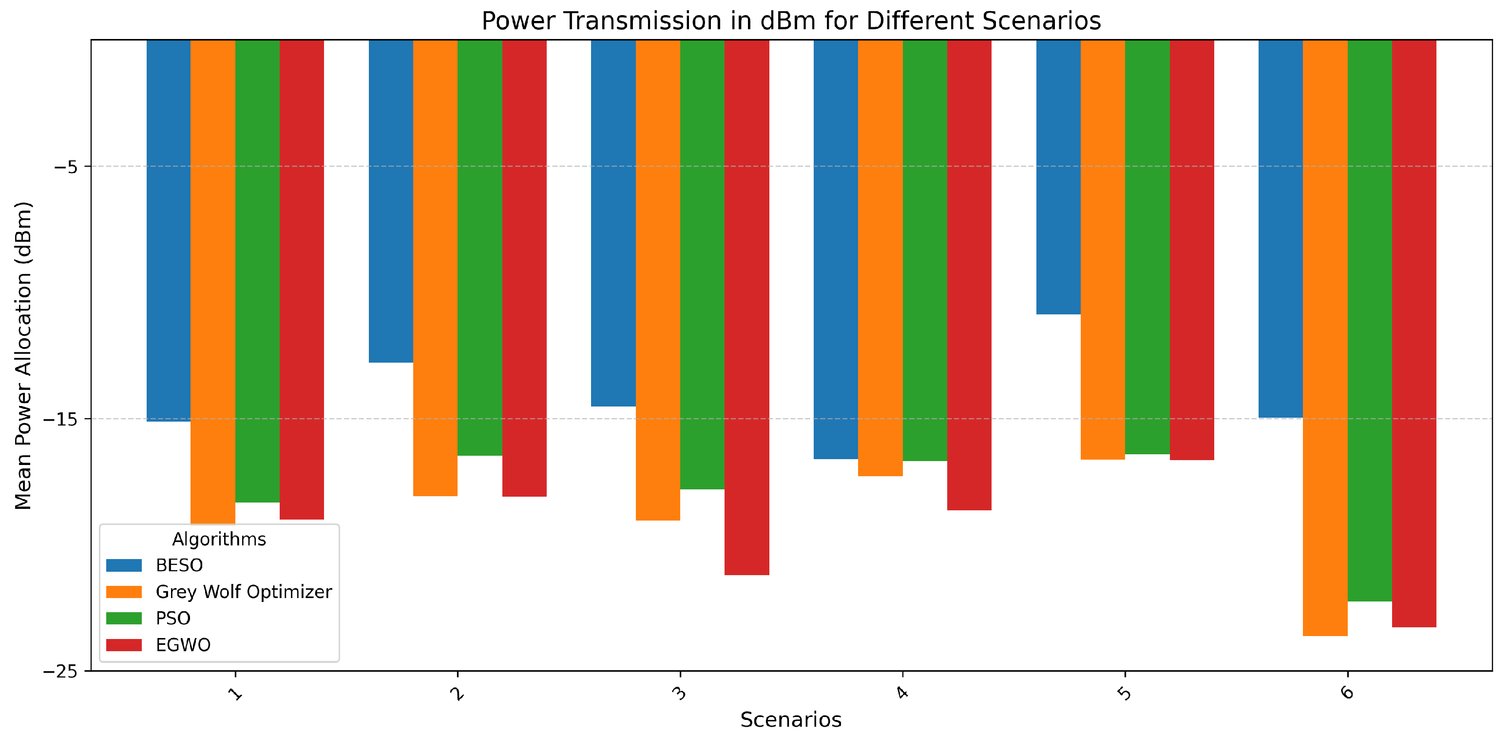
| Algorithm | Scenario | |||||
|---|---|---|---|---|---|---|
| 1 | 2 | 3 | 4 | 5 | 6 | |
| BESO | −15.139 | −12.794 | −14.536 | −16.608 | −10.880 | −14.965 |
| PSO | −18.323 | −16.477 | −17.809 | −16.693 | −16.421 | −22.257 |
| GWO | −19.256 | −18.075 | −19.042 | −17.295 | −16.649 | −23.632 |
| EGWO | −19.011 | −18.113 | −21.216 | −18.652 | −16.657 | −23.288 |
| Algorithm | Scenario | |||||
|---|---|---|---|---|---|---|
| 1 | 2 | 3 | 4 | 5 | 6 | |
| BESO | 30.623 | 52.543 | 35.188 | 21.834 | 81.652 | 31.872 |
| PSO | 14.709 | 22.504 | 16.559 | 21.411 | 22.793 | 5.946 |
| GWO | 11.867 | 15.575 | 12.467 | 18.642 | 21.631 | 4.332 |
| EGWO | 12.557 | 15.441 | 7.556 | 13.636 | 21.59149 | 4.689 |
Disclaimer/Publisher’s Note: The statements, opinions and data contained in all publications are solely those of the individual author(s) and contributor(s) and not of MDPI and/or the editor(s). MDPI and/or the editor(s) disclaim responsibility for any injury to people or property resulting from any ideas, methods, instructions or products referred to in the content. |
© 2025 by the authors. Published by MDPI on behalf of the International Institute of Knowledge Innovation and Invention. Licensee MDPI, Basel, Switzerland. This article is an open access article distributed under the terms and conditions of the Creative Commons Attribution (CC BY) license (https://creativecommons.org/licenses/by/4.0/).
Share and Cite
Fauzan, M.N.; Munadi, R.; Sumaryo, S.; Nuha, H.H. Enhanced Grey Wolf Optimization for Efficient Transmission Power Optimization in Wireless Sensor Network. Appl. Syst. Innov. 2025, 8, 36. https://doi.org/10.3390/asi8020036
Fauzan MN, Munadi R, Sumaryo S, Nuha HH. Enhanced Grey Wolf Optimization for Efficient Transmission Power Optimization in Wireless Sensor Network. Applied System Innovation. 2025; 8(2):36. https://doi.org/10.3390/asi8020036
Chicago/Turabian StyleFauzan, Mohamad Nurkamal, Rendy Munadi, Sony Sumaryo, and Hilal Hudan Nuha. 2025. "Enhanced Grey Wolf Optimization for Efficient Transmission Power Optimization in Wireless Sensor Network" Applied System Innovation 8, no. 2: 36. https://doi.org/10.3390/asi8020036
APA StyleFauzan, M. N., Munadi, R., Sumaryo, S., & Nuha, H. H. (2025). Enhanced Grey Wolf Optimization for Efficient Transmission Power Optimization in Wireless Sensor Network. Applied System Innovation, 8(2), 36. https://doi.org/10.3390/asi8020036