Abstract
Federated learning (FL) enables deep learning models to be trained locally on devices without the need for data sharing, ensuring data privacy. However, when clients have uneven or imbalanced data distributions, it leads to data heterogeneity. Data heterogeneity can appear in different ways, often due to variations in label, data distributions, feature variations, and structural inconsistencies in the images. This can significantly impact FL performance, as the global model often struggles to achieve optimal convergence. To enhance training efficiency and model performance, a common strategy in FL is to exclude clients with limited data. However, excluding such clients can raise fairness concerns, particularly for smaller populations. To understand the influence of data heterogeneity, a self-evaluating federated learning framework for heterogeneity, Fed-Hetero, was designed to assess the type of heterogeneity associated with the clients and provide recommendations to clients to enhance the global model’s accuracy. Fed-Hetero thus enables the clients with limited data to participate in FL processes by adopting appropriate strategies that enhance model accuracy. The results show that Fed-Hetero identifies the client with heterogeneity and provides personalized recommendations.
1. Introduction
Deep learning (DL) models can learn from massive amounts of data, improving automation and performing various tasks without human intervention. Building an efficient deep learning model requires enormous amounts of data and it is essential to highlight the significance of having a large amount of data from relevant categories, particularly when it comes to its critical role in enabling well-informed healthcare decision-making processes. In the healthcare domain, ensuring the privacy of medical data is a significant concern. To address this, a decentralized approach known as federated learning (FL) was developed. FL [1] is a machine learning approach wherein the numerous users distributively or collaboratively train the AI models over remote data centers while keeping data localized. The FL process begins when a server initiates communication with the clients. Each client trains a model using the data available with them and sends the updates to the server, which aggregates all the updates. This approach allows clients to benefit from the insights of other clients’ data without directly sharing their actual data. FL is essential in many applications as it protects sensitive information and provides diversity by collecting data from various locations.
Most existing studies [2,3] compare centralized and federated approaches without considering real-time settings, where data from the same datasets are distributed across different clients. For a federated learning setup to be applicable in real-time settings, the model must be capable of handling data from different geographical locations with varying distributions. Training AI models in heterogeneous and large FL networks presents several challenges such as device heterogeneity, data heterogeneity, and communication overhead [4]. In federated learning, the variability in data distributions among various clients is referred to as data heterogeneity. Data heterogeneity may be due to various reasons, such as incorrect labeling, imbalance in the number of samples, and also due to data collection from multiple sources.
Existing works have explored various federated learning strategies to address data heterogeneity, including assigning higher priority to weights with greater contributions in global updates, enabling them to have a more significant influence on the aggregated model. Techniques such as weighted averaging [5], importance-based aggregation [5], or adaptive weighting [6] are often employed to assign greater importance to clients whose updates significantly impact the global model. Prioritizing clients with larger or higher-quality datasets can enhance the global model’s accuracy. However, if clients with limited data are disregarded or their contributions are reduced, the global model may become skewed toward more prevalent data distributions, reducing its ability to generalize to diverse or rare scenarios. To ensure fair participation, FL systems need mechanisms that balance the importance of well-represented and underrepresented clients. The proposed system, Fed-Hetero, addresses the issue by identifying the type of heterogeneity present in the client data and recommends the clients with limited data to perform data augmentation or clustering, which enhances their contribution to the weight aggregation process.
In the context of healthcare systems, various types of data such as imaging data, patient records, and genetic information can be leveraged for further analysis. This study focuses on heterogeneous data, which is diverse in nature, and investigates the influence of quantity skew, label distribution skew, and image skew. While quantity skew and label distribution skew can be analyzed using any heterogeneous dataset, image skew specifically requires imaging data. Therefore, the study emphasizes on use case of glaucoma prediction, which uses retinal fundus images to explore these skews in detail.
The key contributions of Fed-Hetero are the following:
- Analyze the influence of data volume on federated learning performance in the context of glaucoma prediction using retinal fundus images.
- Identify clients affected by data heterogeneity due to variations in labels, quantities, and image skew.
- Recommend strategies to the clients for addressing data heterogeneity which improves federated learning performance.
2. Related Works
2.1. Federated Learning
The literature survey gives an introduction to FL, challenges faced by FL, and various applications of FL. FL [7,8] is a collaborative machine learning approach where models are trained across multiple devices or servers in a decentralized manner. Instead of sharing data, each client independently performs training on its data and transmits the resulting weights to a server. The aggregation of all the weights from the clients is performed by the server using the Federated Averaging (FedAvg) algorithm to generate a global model. This approach helps to maintain data privacy, as sensitive data do not need to leave the client devices. In certain federated learning studies, the same dataset is partitioned and distributed among multiple clients. While this method is commonly employed in experimental setups, it may not be well-suited for real-world applications [3]. A comparison of FL to centralized learning was carried out [2] and the study demonstrates that the centralized approach delivers superior accuracy in IID setting. Federated learning faces several challenges, including communication overhead, privacy and security concerns, and data distribution issues. One of them is the high communication cost associated with transmitting model weights between clients and the server. This can be exacerbated when large models are involved or when clients are frequently disconnected from the training process due to connectivity issues. While federated learning aims to preserve data privacy, certain vulnerabilities may still exist, particularly when it comes to adversarial attacks or issues related to data leakage during the aggregation process [9]. In many studies, data distribution among clients is considered to be uniformly distributed (IID), which does not reflect real-world scenarios. Non-uniformly distributed (Non-IID) data distribution, where data are uneven or imbalanced across clients, can lead to poorer model performance. This issue has been observed in medical image classification [10], where different clients had varying distributions of labels, affecting model accuracy.
Federated learning has diverse applications, including areas such as healthcare, facial expression recognition, medical image classification, and binary supervised classification. FL has shown great potential in healthcare [11], as it enables the training of models while preserving patient data privacy. Studies have explored how FL can be applied in healthcare data to avoid the high costs and risks associated with centralized data storage. A healthcare-focused federated learning architecture helps to preserve data privacy by keeping sensitive data localized on clients, while the central server only aggregates model updates. A federated learning model was proposed for facial expression recognition in advertisements, allowing a system to predict user interests in real time [12]. A graphical user interface (GUI) was developed to facilitate this real-time prediction, with suggestions to refine feature extraction techniques for better model performance. FL has been applied to medical image classification [10], showcasing its effectiveness in handling distributed datasets. In a federated SVM architecture [13], it was utilized for binary classification tasks using the MNIST and COVID-19 datasets, with results compared to centralized approaches. These comparisons highlighted the limitations of using random data splits across clients, which may not reflect practical real-world scenarios.
2.2. Algorithms for Handling Data Heterogeneity
The literature explores several studies in the area of data heterogeneity, emphasizing different types such as quantity skew, label distribution skew, feature skew, and image skew. It also explores various strategies for addressing data heterogeneity [14]. These algorithms can be classified as client-side or server-side approaches and few researchers have looked into developing personalized solutions [15] for the same. Data heterogeneity [16] poses a significant challenge in federated learning, as it reduces model effectiveness across diverse client devices. Data heterogeneity may be due to various factors such as variations in data distribution, client device capabilities, and communication constraints. These challenges hinder the aggregation of local models into a global model that performs effectively across all clients. Quantity skew refers to an imbalance in the number of data samples distributed among clients. Some clients may have large amount of data, while others have significantly smaller amounts of data. This imbalance can result in poorly generalized global models, as clients with limited data contribute less effectively to model training. Feature skew occurs when clients have different sets of features, with each client potentially holding only a subset of the features necessary for training. This can cause difficulties in model convergence and performance consistency across clients. Label distribution skew refers to situations where the distribution of labels varies across clients. Some clients may have an over-representation of certain classes, while others may be biased toward other classes. This imbalance can lead to poor global model performance, especially on underrepresented classes.
Federated recommendation systems (FedRS) represent a promising application of federated learning, addressing key factors such as privacy, security, heterogeneity, and communication costs. Recent research, as highlighted in the survey [17], provides a detailed comparison of various approaches and solutions in the context of federated recommendation systems. This research also identifies promising future directions for advancing the field. With their substantial potential, federated recommendation systems represent a field that requires further development and exploration to improve personalized recommendations while ensuring privacy and reducing communication overhead.
To address quantity skew, solutions such as Zero-shot Data Generation (ZSDG) have been introduced [18]. ZSDG generates synthetic labeled data based on knowledge learned from trained models, helping to augment the data at the client level without requiring real data. The data produced by the global model may be limited by the knowledge they have already acquired. This can result in synthetic data that closely resemble the original training data, reducing their diversity and novelty. Another limitation of this work is that the starting point for data augmentation has been considered only in terms of local epochs, whereas federated learning rounds should also be taken into account.
Federated Feature Distillation (FedFed) [19] handles feature skew by categorizing features into performance-robust and performance-sensitive groups. By focusing on sharing only performance-critical features, FedFed helps to mitigate the effects of feature mismatch among clients, but it introduces communication and storage overheads, and poses potential privacy concerns. Federated Augmented Feature Learning (FedAF) [20] tackles label distribution skew by enabling clients to share condensed data and soft labels with the server. By focusing on the most essential data points for training, FedAF mitigates the impact of label distribution skew; again, privacy might remain a concern. FedICON [21] uses contrastive learning to address data variability over time and between clients, focusing on extracting invariant features to tackle shifts in image data and other modalities. The FedLAW [5] approach uses a weight shrinking concept which is applied to the aggregation weights used in federated learning. These weights determine the contribution of each client’s model updates during the aggregation process to form the global model. This adjustment impacts the influence of individual client updates on the global model by excluding the clients with lesser weights.
FLAMA (Federated Learning with Adaptive Weighted Model Aggregation) [6] dynamically adjusts the model aggregation weights in each federated learning training round, considering the number of useful data samples contributed by each client and the performance of the global model. Clients with fewer or less useful data samples might receive lower aggregation weights, potentially marginalizing under-represented data distributions.
The one-pass distribution sketch [22] analyzes the variations in data distributions among clients, selects clients based on these differences, and personalizes tasks accordingly. The client selection strategy excludes the clients with limited data. Federated daisy chaining [23] enables clients to share information with other clients via a server, which raises privacy concerns. Table 1 presents the summary of the federated learning algorithms and their limitations.

Table 1.
Summary of existing works.
The observations from the related works are given below:
- The main challenges in federated learning are data heterogeneity, communication overhead, and privacy concerns.
- Data heterogeneity can occur due to various factors, including quantity imbalance, label distribution imbalance, feature variability, and image variation.
- Various algorithms are proposed to address the quantity skew, label distribution, and feature skew data heterogeneity.
- In most existing studies, the same datasets are shared among different clients, which does not accurately reflect real-world scenarios.
The limitations of the existing works are as follows:
- The literature reveals that most existing studies tend to exclude the clients with limited data by using strategies such as weighted averaging, importance-based aggregation, or adaptive weighting.
- Most approaches use an information-sharing strategy that compromises privacy and performs client selection and personalization based on data distributions.
- The existing works have not fully explored the potential of a server-based feedback system to notify clients with reduced performance.
3. Notations and Preliminaries
This section explains the fundamental concepts of federated learning along with the associated terminologies for Fed-Hetero. Section 3.1 discusses federated learning, Section 3.2 focuses on data heterogeneity, and Section 3.3 deals with metrics used to measure data heterogeneity. Section 3.4 deals with recommendations suggested to clients.
3.1. Federated Learning
Consider an FL system with m clients, each having distinct distributions of data. The clients used for this study are represented as client 1, …, client m. Each client is associated with distinct datasets represented as D with n samples distributed across K classes which are divided into training and testing data. Let
be the data where denotes the features of the i-th sample, and class is denoted as . A local model trained by each client m using the dataset D. Once the training is complete, the parameters of the local model are sent to the server for aggregation. These parameters are combined by server to update the global model. The objective of federated learning can be represented as minimizing the global loss function with model parameters w and loss function for client i :
where is the total number of samples in all clients.
3.1.1. Local FL Model
The local model is trained on data from individual clients and local accuracy measures the performance of a model trained specifically on a client’s local data. Let:
- : Local dataset of a client (with n samples).
- : The actual label for the i-th sample in .
- : Predicted label for the i-th sample by the local model.
The formula for calculating local accuracy is
where is a binary function that outputs 1 if the predicted label matches the true label and 0 otherwise.
3.1.2. Global FL Model
The global model is an aggregated version of the local models, created by combining the weights gathered from all participating clients. Global accuracy measures how well the global model (aggregated from multiple clients) performs on a specific client’s local dataset. Let:
- : Aggregated weights from multiple clients.
- : Predicted label for the i-th sample using the global model.
The formula for calculating global accuracy is
3.1.3. FedAVG
FedAvg is a basic algorithm in federated learning that balances the need for collaborative model training with the requirement for data privacy. Algorithm 1 shows the working of FedAVG [7]. After the first client server interaction, the server collects the updated model parameters from the selected clients. The server computes the new model parameters by averaging the model parameters received from clients. The aggregation is usually performed using a weighted average, using the weights corresponding to the number of samples on each client.
| Algorithm 1 Federated Learning Algorithm |
|
3.2. Data Heterogeneity
In FL, data heterogeneity refers to the differences in data distributions across various clients. Heterogeneous data refer to data collected from diverse sources and presented in various formats, differing in quantity and labeling. Heterogeneity can manifest in different forms, such as quantity skew, label distribution skew, and image skew. These factors can significantly influence both the training process and the performance of the resulting model. Various types of heterogeneity are discussed in the following sections.
3.2.1. Quantity Skew
The uneven distribution of data samples in different clients is known as quantity skew. This skew arises when certain clients have considerably more data than others, which can impact the training process and model performance.
3.2.2. Label Distribution Skew
The uneven distribution of classes across different clients is referred to as label distribution skew. This skew occurs when certain clients have a disproportionate representation of specific labels, leading to challenges in training a robust and generalized model.
3.2.3. Image Skew
Image skew refers to differences in luminance, contrast, and structural information of images across different clients. Variations in the structural representation can impact the training accuracy of federated learning models.
3.3. Metrics to Measure Data Heterogeneity
3.3.1. Weight Divergence
Weight divergence between clients is a technique used in FL to assess and monitor variations in model updates sent to the server by different clients. This approach provides the server with insights into the consistency of model updates, acting as an indicator of model performance, convergence, or accuracy. When the divergence is minimal, it implies that the model is performing uniformly across the various clients.
The weight divergence for the client i can be defined as follows:
where:
- : Weight divergence for client i.
- : Model weights from client i.
- : Aggregated global model weights.
- : L2 norm (Euclidean distance) of the difference between two weight vectors.
3.3.2. Jensen–Shannon Divergence (JSD)
Jensen–Shannon Divergence (JSD) [24,25] is a statistical measure used to compare similarity between two probability distributions. This helps to find how similar class distributions are between a pair of distributions. The Jensen–Shannon Divergence between two probability distributions S and R is defined as follows:
where:
- is the average of the two distributions.
- is the Kullback–Leibler divergence from S to M:
- is the Kullback–Leibler divergence from R to M:
JSD range values are displayed in Table 2.
Table 2.
JSD threshold.
A JSD value near zero indicates similar distributions, and as the value moves toward 1, it indicates dissimilar distributions. The choice of the upper-limit threshold is specific to the dataset used in the study. The details of the threshold are given in the Experiment Setup section in Section 5.
3.3.3. Sub Sample Sharing
The sub-sample sharing refers to a strategy where clients selectively share small portions (sub-samples) of their local datasets with the central server. Each client i holds a local dataset , which contains input–label pairs:
where is the input data sample, is the corresponding class, and is the number of samples in the dataset.
Client i selects a subset for sharing.
where is the index set of the selected sub-samples. This allows clients to limit the amount of data they share while still contributing to the improvement in the global model.
3.3.4. Structural Similarity Index
The Structural Similarity Index (SSIM) [26] is a measure used to compare and quantify the similarity between two images. It evaluates differences in structural details, factoring in elements such as brightness, contrast, and overall structure. The SSIM index is calculated using the following formula as defined in [26].
where the variables used in Equation (8) as defined in [27] are the following:
- are the average values of the images y and z.
- are the variances of the images y and z.
- is the covariance of y and z.
- and are small constants.
The similarity range is shown in Table 3.
Table 3.
SSIM similarity range.
An SSIM value of 1 indicates perfect similarity (identical images), 0 means no similarity, and values closer to 1 indicate greater similarity. The threshold values are specific to the dataset used in the study to identify clients with close similarity and details are mentioned in the Experiment Setup section in Section 5.
3.4. Recommendations
The server notifies the clients about the type of heterogeneity present in their data and recommends strategies to address the heterogeneity. The recommendations send to clients are denoted as , which indicates quantity skew, means label distribution skew, and means image skew. Data augmentation and clustering are the strategies recommended based on the type of data heterogeneity associated with client data. The recommendations based on JSD and SSIM are shown in Equations (9) and (10).
4. System Architecture
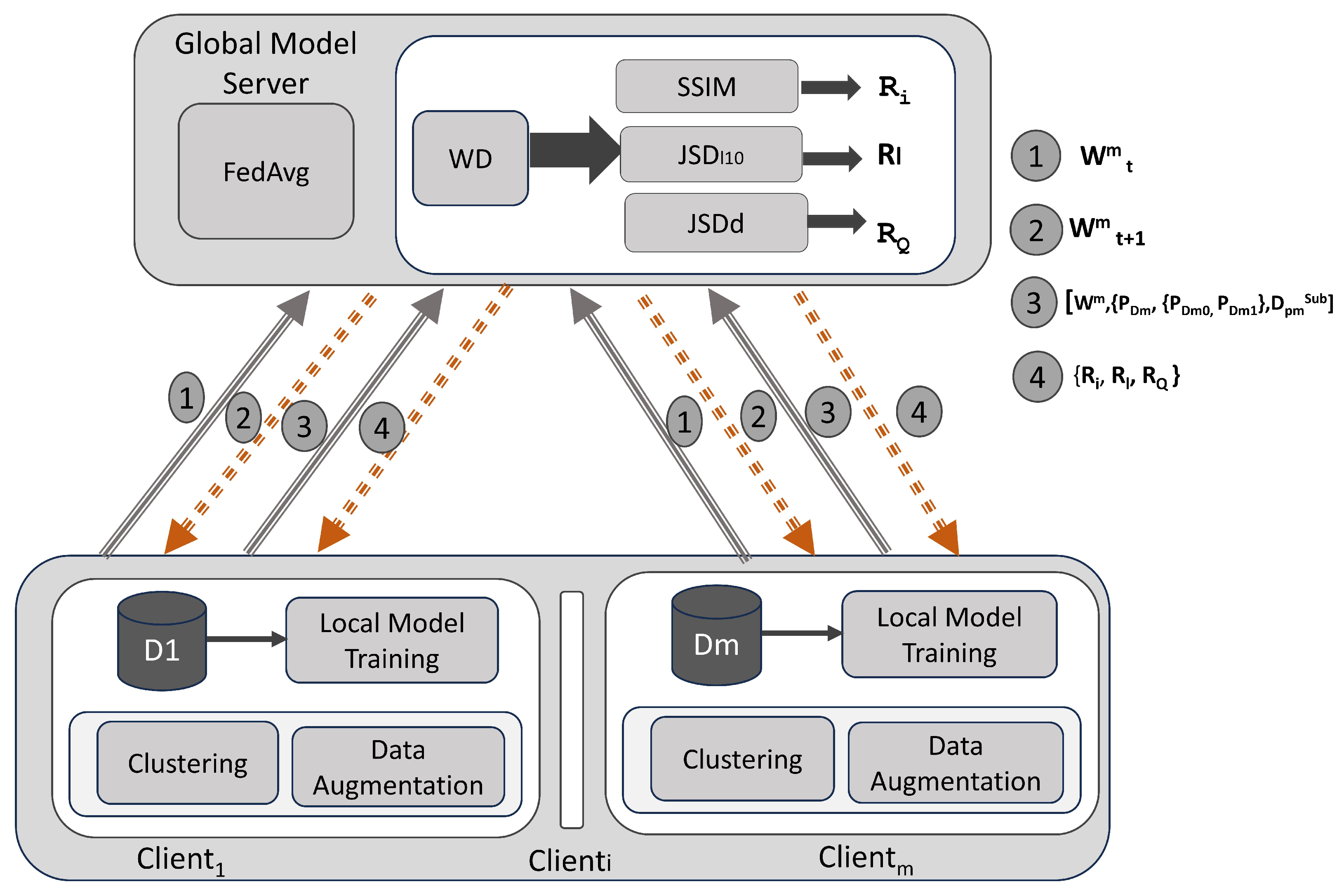
Fed-Hetero is a self-evaluating framework that provides recommendations to clients, guiding them to perform clustering or data augmentation to enhance accuracy whenever the performance of federated learning is decreased due to the diversity in the data. Fed-Hetero enables clients with limited data to actively participate in the FL process by employing appropriate strategies that improve the accuracy of the model. Clients with limited data may represent rare or critical cases and also provide valuable insight that is essential to improve the generalization of the model in diverse scenarios. The federated learning process begins when the server makes a request to the clients with initial global model parameters . The clients participating in the study, ranging from client 1 to client m (where m = 4), train the CNN model. Each client then sends its model weights (where “t” indicates the number of rounds) to the server, which uses the FEDAVG algorithm to aggregate the weights and sends to the clients after each round. After “nt” rounds of the federated learning process, the server calculates the weight divergence (WD) factor between clients. Based on WD, the server requests the data distributions, subset of samples from each client. The client then sends the probability of data distributions—PDm, probability distributions between classes—PDm0, PDm1, and subset of samples—, and the server computes the JSD between clients—, JSD between classes in the clients—, and SSIM between the subset of images from the clients—SSIM values. The server notifies the clients about the heterogeneity present in their data and recommends data augmentation and clustering to mitigate it. The system architecture diagram in Figure 1 illustrates the flow of communication and data exchange between the clients and the server during the federated learning process.
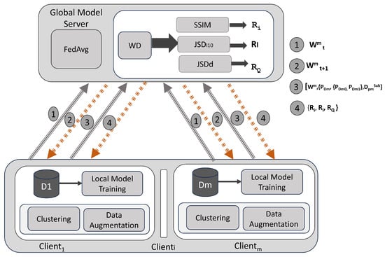
Figure 1.
System architecture for Fed-Hetero recommendation system for clients.
Fed-Hetero Algorithm
This section presents a comprehensive overview of the modules in Fed-Hetero. The process begins with Algorithm 2, which serves as the foundational step for the self evaluating framework. Algorithm 2 is composed of several sub-modules designed to handle specific tasks. The sub-modules functionalities are specified in Algorithms 3–6. Algorithm 3 identifies the weight divergence between the clients, followed by Algorithm 4 for estimating quantity skew, Algorithm 5 for computing label distribution skew, and Algorithm 6 for identifying image skew. These algorithms estimate the type of heterogeneity associated with data in the clients and recommend strategies to mitigate it.
| Algorithm 2 FEDHetero |
|
| Algorithm 3 Weight_Divergence( |
|
| Algorithm 4 JSD(PDm) |
|
| Algorithm 5 JSD(PDm0, PDm1) |
|
| Algorithm 6 SSIM() |
|
5. Experiment Setup
This section provides a detailed discussion of each module in Fed-Hetero, the self-evaluating framework which estimates the type of heterogeneity present in each client and suggests appropriate measures to reduce it. It includes the dataset details in Section 5.1, client and server modules in Section 5.2 and Section 5.3, and the mathematical definitions for estimating quantity skew, label skew, and image skew in Section 5.4 and finally discusses the recommendation module in Section 5.5 and the ablation study in Section 5.6.
5.1. Dataset Description
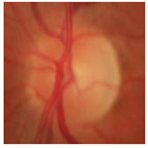
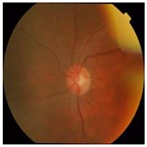
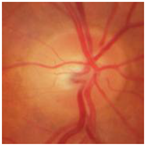
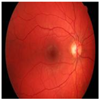
The datasets considered for the study include retinal fundus images for glaucoma prediction. The datasets are denoted as , , , and where k = 4 with the same K classes associated with client 1 to client m where m = 4. The datasets considered for the study are Riga [30] , Dhristi [31], Rim-one [32], and HRF [33]. These datasets consists of two classes, class 0 for non-glaucoma and class 1 for glaucoma. Table 4 show the details of the datasets used for the study.
Table 4.
Dataset details.
Data pre-processing is performed in all clients to convert all dataset images into standard format because they may vary in size. To bring all images to the same size, a rescale function is used, which normalizes all pixel values to the range [0, 1]. A 20% shear and zoom ise applied to the images on all clients as an initial pre-processing step.
This study could be expanded to incorporate eye-tracking datasets, as they also exhibit quantity skew due to the limited number of images. The experiment can also be conducted on the optic disc detection dataset, which includes radiologists’ gaze patterns as they locate optic discs in retinal fundus images [34,35,36]. Another dataset related to eye-tracking data focuses on analyzing how individuals with glaucoma navigate their environment, specifically examining how they perceive and process visual stimuli [37].
5.2. Fed-Hetero Client Local Models
The clients client 1 to client m, where m = 4, train the models locally with the data associated with them. The model used for training is a CNN network which consists of six layers; the first four are convolutional and pooling, and the last two are fully connected. The convolutional layer has 32 filters of kernel size 3, and the activation function used is ReLu. Subsequently, max pooling is employed to decrease the spatial dimensions of the output volume. The last layer is the fully connected layer which predicts as glaucoma or non-glaucoma. At defined intervals, a local update is generated and transmitted from each client to the server. The Fed-Hetero local model architecture is shown in Table 5.
Table 5.
Fed-Hetero local model.
5.3. Fed-Hetero Server Global Model
The server sends the initial global parameters to all clients. After each round of federated learning process, a server accumulates the weights from the clients and computes their average, and integrates it into the evolving global model. These improved global model parameters are returned to the clients, who employ it to conduct further training in subsequent communication rounds. Iterations persist until the desired level of convergence is achieved or the predetermined communication rounds are concluded, ensuring a cooperative and iterative learning process. After “nt” rounds, the server calculates the weight divergence for each client to see how far their local updates differ from the new aggregated global model.
5.4. Data Heterogeneity Estimation
To understand type of data heterogeneity associated with each client and to provide recommendations, we focus on measuring the quantity skew, label distribution skew, and image skew.
5.4.1. Estimate Quantity Skew
After a specified number of rounds “nt” based on the weight divergence factor, the server accepts the additional parameters such as , where l = 0, 1, along with the where m= client 1 to client 4. The class distributions of client 1 to client 4 are given below:
Here, , , , is the probability of class c in dataset , , , . All clients calculate the probability distributions of the data they possess. Each client has an , which is then sent to the server. The server computes the for the datasets from client 1 to client 4.
The Jensen–Shannon Divergence (JSD) between the four class distributions , , and is defined as follows:
where i and j can be any of the dataset pairs from , , , .
JSD between each client pairs is calculated as shown in Equations (16)–(21).
where is the Kullback–Leibler Divergence [38] as shown in Equations (22)–(25).
JSD is used to evaluate the differences in data distributions across multiple clients. A smaller value indicates that the clients have similar distributions and larger value indicates greater dissimilarity. The reported upper-limit thresholds are specific to the dataset used in the study to identify clients with close similarity, with 0.4 determined as the upper limit for JSD and the lower limit 0. Based on the value as shown in Equation (26), the server can notify the clients using about the type of heterogeneity associated in their data, prompting them to explore methods such as data augmentation [28] for improving the accuracy of their individual models.
5.4.2. Estimate Label Distribution Skew
To estimate label distribution skew, based on the weight divergence factor the server requests the probability distribution for each class from all the clients. The comparison of the label distributions using the Jensen–Shannon Divergence (JSD) is given below as follows:
Let and represent the probability distributions of class 0 and class 1 in client m, respectively, where m = no. of the clients.
The probabilities can be defined as follows:
where is the count of instances for class i in client m, and is the total number of instances in client C. Each client computes the and , which is then sent to the server. Based on the probabilities received from the clients, the server calculates the JSD between the four distributions for each class as follows:
, , , are the probability distributions for class 0 and class 1 in datasets , associated with clients 1 to m where m1, m2 represent a pair of clients. and are calculated for each class. Assume that the distributions , for class 0, and , for class 1 over the same domain .
For Class 0, compute the average distribution:
Compute the KL divergences for Class 0:
Compute the Jensen–Shannon Divergence for Class 0:
Similarly, compute the average distribution for Class 1:
Compute the KL divergences for Class 1:
Compute the Jensen–Shannon Divergence for Class 1:
JSD [39] is a measure of similarity between two probability distributions. A JSD value near to zero indicates similar distributions and, as the value moves toward 1, this indicates dissimilar distributions. Based upon the , value of each classes 0, 1 as shown in Equations (35) and (36), the server can provide recommendations to clients such that they can improve the number of samples with respect to each class using data augmentation [28].
5.4.3. Estimate Image Skew
To measure the image skew data heterogeneity, a predefined subset of samples is shared from the clients to the server. The subsets are represented as s1, s2, s3, s4 such that . The server calculates the SSIM between the images in the samples SSIM(I_1,I_2) to SSIM(I_3,I_4) using samples drawn from s1, s2, s3 and s4.
SSIM values vary from 0 to 1 and a value close to 1 indicates high similarity between images. The range selected for the study considered a higher limit as 1 indicating that the two images are identical and a lower limit as less than 0.8 meaning that the images have significant differences. In medical use cases, it is preferable to consider images with greater similarity, meaning SSIM values should be as close to 1 as possible. We set the threshold at 0.8, as it was the highest value observed in the study. We also examined existing studies [40] that utilized SSIM to assess the structural similarity of medical images, which also define the SSIM range. The threshold obtained and discussed in Fed-Hetero has been validated with the chosen dataset. Detailed investigations of extending on different datasets to fix the thresholds adaptively have not been considered in the current study.
Based on SSIM value as shown in Equation (37), the server recommends the clients about image skew and also mentions the clients which it has to cluster [29].
5.5. Recommendations
Based on , , and SSIM values, the server sends the recommendations , , and to the clients. The clients with limited representation in the global update are informed about their low contribution, encouraging them to include methods like data augmentation [28] and clustering [29] to enhance their participation in future global updates.
5.6. Ablation Study
We aim to explore the the effect of changing the number of local training epochs (local training steps) on global rounds. The experiment was conducted by altering the number of local epochs while keeping the number of global rounds fixed at 3. The local epochs considered are E = 30, 50, 70. It is observed that clients with limited data do not experience an improvement in accuracy. In fact, their accuracy either remains unchanged or decreases.
Hyperparameter tuning was performed using Optuna over 20 trials to identify the optimal values for learning rate, epochs, and batch size. The best-performing model from this process was saved and later employed for training in a federated learning setup. However, when each client utilized its optimized model, the performance of the federated learning approach declined, potentially due to non-IID data characteristics. This performance degradation might be attributed to quantity skew and image skew. From both investigations, it is evident that data augmentation or clustering is necessary to enhance performance.
6. Results and Discussions
Fed-Hetero provides recommendations to clients on the type of heterogeneity present in the data. Based on type of heterogeneity, data augmentation or clustering is recommended to clients, which improves the FL performance. The subsections explore the performance of federated learning as outlined in Section 6.1, the heterogeneous nature of data associated with clients highlighted under Section 6.2, the factors influencing client performance detailed in Section 6.3, recommendations presented in Section 6.4, and a comparison with existing works discussed in Section 6.5.
6.1. Performance of Fed-Hetero
The performance of Fed-Hetero for local and global accuracy after three rounds is shown in Table 6 and Table 7. Its noticed that the global accuracy of client 2 and client 4 is not improving, prompting an investigation into the type of data skew affecting the performance of the federated learning models. The server notifies the clients with the type of data heterogeneity and recommends the clients to perform data augmentation or clustering.
Table 6.
Local accuracy for clients across three rounds.
Table 7.
Global accuracy for clients across three rounds.
6.2. Heterogeneous Nature of Data
The Table 8 displays sample images from the datasets [30,31,32,33] to highlight the variations in the structural patterns of the images.
Table 8.
Heterogeneous data selected for Fed-Hetero [30,31,32,33].
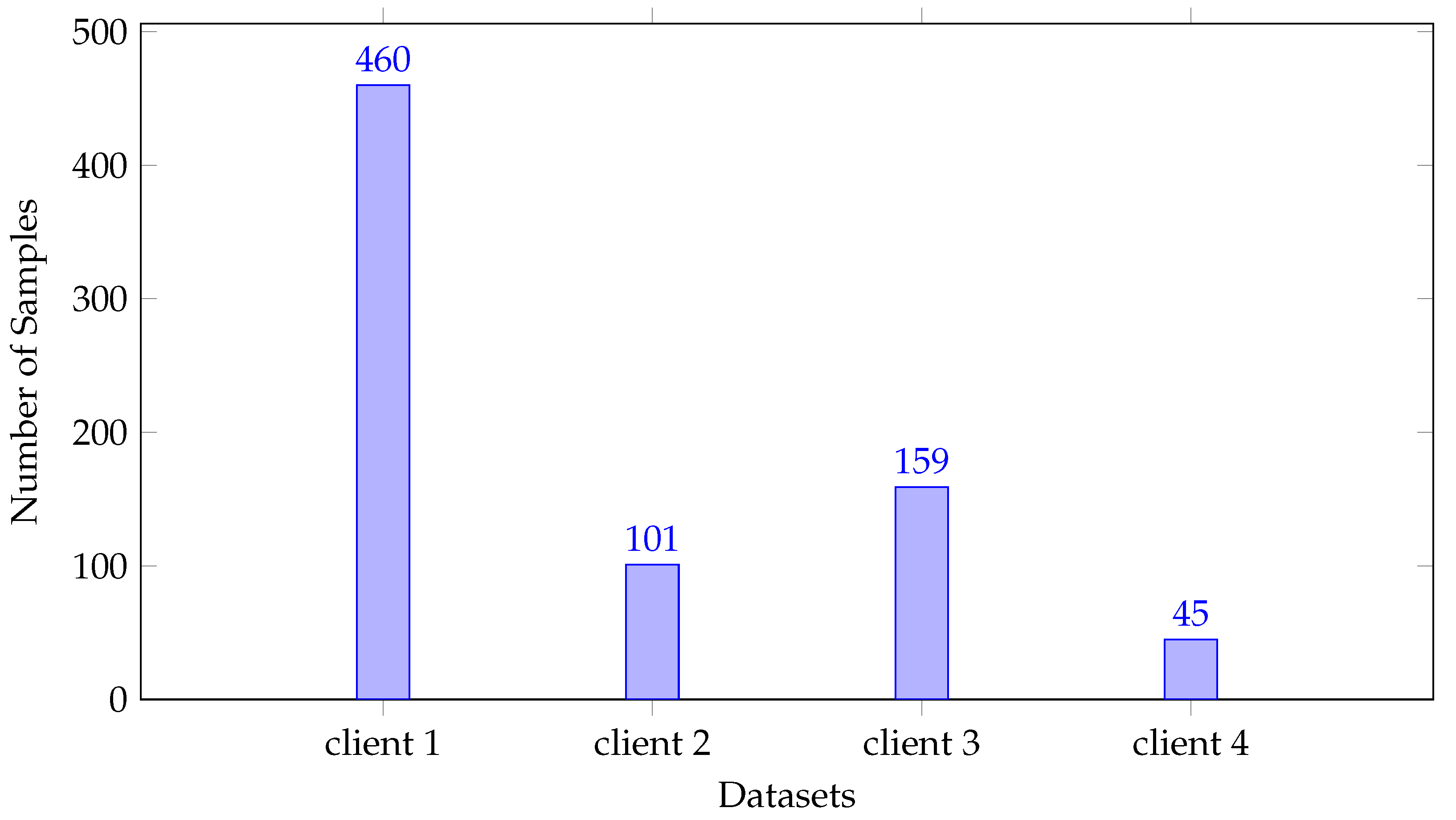
To analyze the heterogeneity in the data associated with clients, we plotted the images based on the quantity shown in Figure 2.
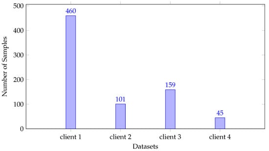
Figure 2.
Heterogeneous nature of data with respect to quantity skew.
6.3. Heterogeneous Factors Effecting Client Performance
The effect of different skewness levels on the data was analyzed by examining the distribution of quantities, labels, and image skew.
6.3.1. Quantity Skew
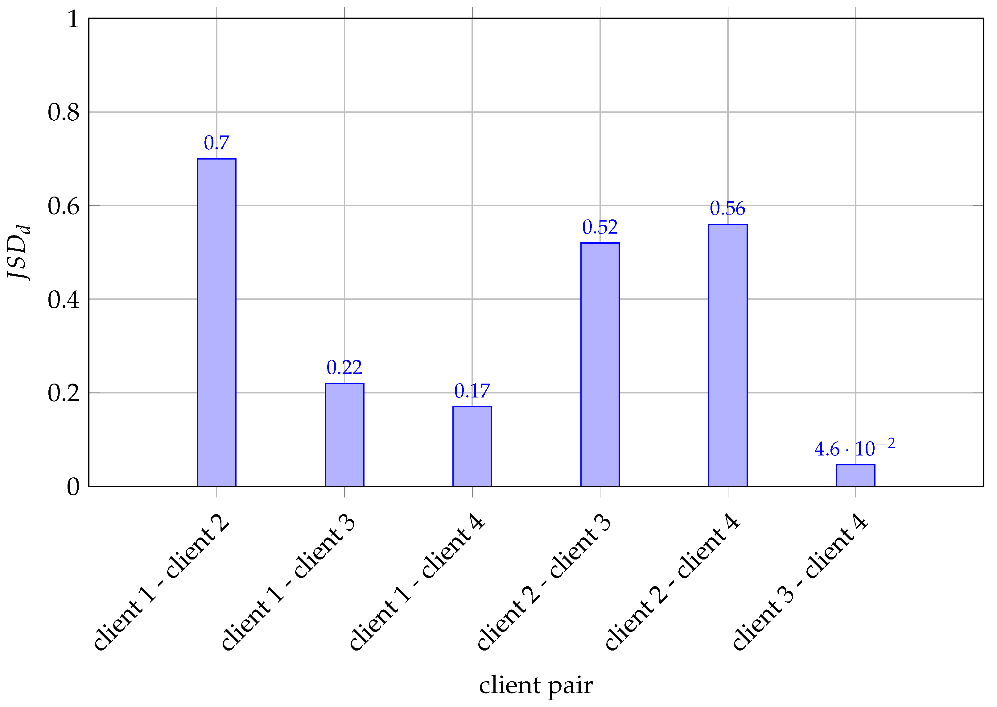
To understand the effect of quantity skew on the overall performance of FL values between the samples in the clients are computed by the server and results are shown in Table 9.
Table 9.
Evaluation of quantity skew based on JSD between clients.
The inference from the Figure 3 and Table 9 (shown in bold) is that the Jensen–Shannon Divergence (JSD) values of client 2 with client 1, client 3, client 4 indicate a high level of divergence. This indicates that client 2 exhibits significant differences from client 1, client 3, and client 4 in their distributions. Such critical divergence implies that the underlying patterns or behaviors within client 2 differ substantially from those observed in client 1, client 3, and client 4. Hence, we can infer that the decrease in global accuracy is attributed to the participation of client 2.
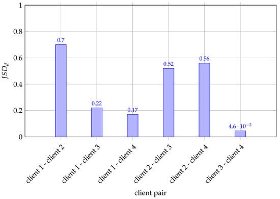
Figure 3.
Evaluation of quantity skew based on JSD between clients depicted in bar graph.
6.3.2. Label Distribution Skew
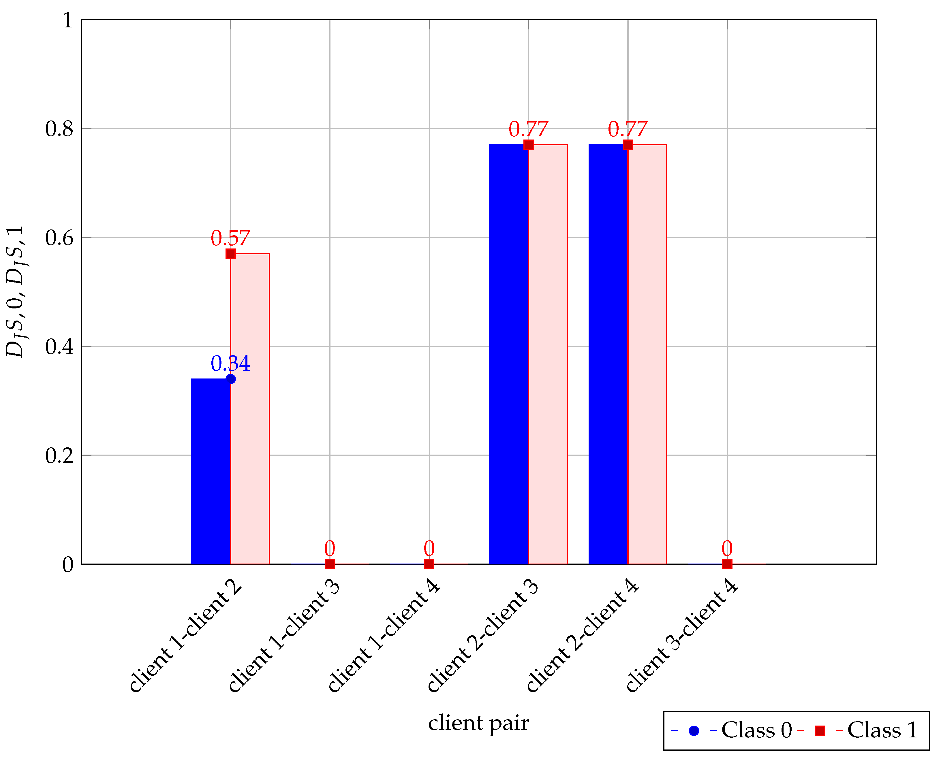
The label distribution skew impact on the FL accuracy is assessed by calculating the JSD between the classes(class 0 and class 1) , for the samples associated with the clients. Table 10 displays the JSD values between classes in the clients to evaluate label distribution skew.
Table 10.
Evaluation of label distribution skew based on JSD between clients.
A JSD value below 0.1 suggests that the data associated with the clients are similar, while a value greater than 0.4 indicates significant dissimilarity. The results, as shown in Figure 4 and Table 10 (in bold), show significant divergence in the label distributions for client 2 with other clients for classes 0 and 1. Thus, we can infer that client 2 participation in the FL process affects the accuracy of the FL model.
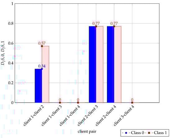
Figure 4.
Evaluation of label distribution skew based on JSD values between clients depicted in bar graph.
6.3.3. Image Skew
To evaluate image skew, the SSIM values are computed for the subset of images which is shared to the server which is shown in Table 11.
Table 11.
Evaluation of image skew based on SSIM values between clients.
The inference from the study is that the clients client 1–client 3, client 2–client 4 have good similarity, which indicates that they contain similar type of images. Client 2 exhibits both quantity skew and label skew. Table 12 shows the inferences from the JSD and SSIM across the clients.
Table 12.
Evaluation of various skews across clients in Fed-Hetero.
6.4. Recommendations-, and
, , and are the recommendations given to the client from the server. indicates quantity skew, refers to label distribution skew, represents image skew. Based on this inference, to reduce the amount of data heterogeneity, the client performs data augmentation or clustering. The recommendations mentioned for each client are shown in Table 13. Based on , , and SSIM values, similarity in the distributions can be identified. The distributions of client 1 and client 3 are similar. Likewise, client 2 and client 4 exhibit a similarity in their distributions. Thus, clustering is recommended for client 1 and client 3, client 2 and client 4. As the for client 2 with other clients is 0.5 to 0.7, which indicates higher divergence, the data augmentation [28] is recommended for client 2.
Table 13.
Recommendations by Fed-Hetero system to the clients.
Data augmentation can be achieved through various strategies, including the use of synthetic data or basic transformations. However, when a synthetic data generator is used to address data heterogeneity, there is no statistically significant evidence that it outperforms standard baselines in correcting class imbalance [41]. Nonetheless, some studies [42] suggest sharing synthetic data generated by clients with other participating clients. Additionally, other research explores a method where a client utilizes a foundation model [43] to generate synthetic data based on its local dataset. A subset of this synthetic data is then transmitted to a central server, which aggregates it into a global synthetic dataset. The server subsequently redistributes this dataset to clients, allowing them to enhance their local data with more diverse and high-quality synthetic samples. While careful generation and distribution of synthetic data can help mitigate under-representation in augmented datasets, it may also raise privacy concerns.
The results after data augmentation with basic augmentation operations show a 10% improvement in accuracy for clients with limited data. The experiment should be extended to include more communication rounds in order to assess whether there is a further increase in accuracy. This could be explored as part of future work. The clustering of clients based on structural similarities in their images was proposed as a direction for future research.
6.5. Comparison with Existing Works
The proposed work Fed-Hetero addresses quantity skew, label distribution skew, and image skew. FL-Hetero explored a client-based approach where clients are informed about the type of data heterogeneity, enabling them to perform either data augmentation or clustering with other clients of similar distributions. Rather than excluding clients with limited data, we focused on incorporating them effectively into the FL process and, instead of sharing information with all clients, it is shared only with servers.
In the work [22], the clients are selected for the FL process based on the similarity in the data distributions. The Federated Feature distillation (FedFed) [19] tackles the data heterogeneity by generating and sharing performance-sensitive features. FedFed raises potential privacy concerns as important features are shared. In federated daisy chaining [23], a daisy chain of local datasets enables more efficient training in data-sparse domains. The clients are sharing information with other clients that do not maintain privacy. Table 14 shows the comparison of Fed-Hetero with the existing works. Most existing works are focused on quantity skew and label distribution skew.
Table 14.
Comparison of existing works with Fed-Hetero.
Fed-Hetero additionally addresses image skew and incorporates a strategy for including clients with limited data into the FL process where the existing works exclude the limited data clients [22]. Fed-Hetero does not address feature skew, which refers to the potential mismatch or imbalance between the features of training and testing data that could affect the model’s generalization performance. The scalability of this approach presents an opportunity for further exploration, particularly in scenarios with a growing number of clients and increased communication rounds in federated learning.
7. Conclusions
A substantial amount of private data remains confined within clients, largely due to privacy and security concerns. Federated learning frameworks generally achieve high accuracy, but their performance may occasionally decline due to data heterogeneity, particularly when dealing with unbalanced and non-IID data distributions. This research aims to explore the impact of data heterogeneity, including quantity skew, label distribution skew, and image skew, on the performance of federated learning, particularly when working with limited data. The proposed work Fed-Hetero, a self-evaluating framework, recommends strategies for addressing data heterogeneity by first identifying the specific type of heterogeneity associated with client data. Fed-Hetero evaluates client performance and recommends techniques such as data augmentation or clustering to enhance outcomes. This ensures the inclusion of clients with limited data in the federated learning process. This study can be expanded to incorporate the feature distribution skew and analyze its impact on the performance of the federated learning setup. Transferring a subset of images to the server for estimating data skewness raises privacy concerns; therefore, we plan to explore privacy-preserving methods as part of our future work.
Author Contributions
Conceptualization, A.M.K. and A.J.; methodology, A.M.K.; software, A.M.K.; validation, A.J.; formal analysis, K.R., G.G., and A.J.; investigation, A.M.K. and A.J.; resources, A.M.K.; writing—original draft preparation, A.M.K.; writing—review and editing, A.M.K. and A.J.; visualization, A.M.K. and A.J.; supervision, K.R. and A.J.; project administration, K.R., G.G. and A.J. All authors have read and agreed to the published version of the manuscript.
Funding
This research received no external funding.
Institutional Review Board Statement
Not applicable.
Informed Consent Statement
Not applicable.
Data Availability Statement
Data are contained within the article.
Acknowledgments
The authors express their gratitude to the “Artificial Intelligence for Health and Well-being” Thrust Area Group within the Department of Computer Science and Engineering (Dept of CSE), Amrita School of Computing, as well as Amrita Vishwa Vidyapeetham, for their invaluable assistance and guidance throughout the study.
Conflicts of Interest
The authors state that there are no conflicts of interest to disclose, and all authors have approved the manuscript and consent to its submission.
References
- Rieke, N.; Hancox, J.; Li, W.; Milletari, F.; Roth, H.R.; Albarqouni, S.; Bakas, S.; Galtier, M.N.; Landman, B.A.; Maier-Hein, K.; et al. The future of digital health with federated learning. NPJ Digit. Med. 2020, 3, 119. [Google Scholar] [CrossRef] [PubMed]
- Liu, J.C.; Goetz, J.; Sen, S.; Tewari, A. Learning from others without sacrificing privacy: Simulation comparing centralized and federated machine learning on mobile health data. JMIR mHealth uHealth 2021, 9, e23728. [Google Scholar] [CrossRef]
- Peng, S.; Yang, Y.; Mao, M.; Park, D.S. Centralized Machine Learning Versus Federated Averaging: A Comparison using MNIST Dataset. KSII Trans. Internet Inf. Syst. 2022, 16, 742–756. [Google Scholar] [CrossRef]
- Li, T.; Sahu, A.K.; Talwalkar, A.; Smith, V. Federated Learning: Challenges, Methods, and Future Directions. IEEE Signal Process. Mag. 2020, 37, 50–60. [Google Scholar] [CrossRef]
- Li, X.; Zhang, S.; Wang, W. Revisiting Weighted Aggregation in Federated Learning with Neural Networks. arXiv 2023, arXiv:2302.10911. [Google Scholar]
- Gao, Y.; Lee, K.; Kim, J. Federated Learning with Adaptive Weighted Model Aggregation. In Proceedings of the 2023 IEEE/ACM 31st International Symposium on Quality of Service (IWQoS), Orlando, FL, USA, 19–21 June 2023. [Google Scholar]
- McMahan, H.B.; Moore, E.; Ramage, D.; y Arcas, B.A. Federated Learning of Deep Networks using Model Averaging. arXiv 2016, arXiv:1602.05629. [Google Scholar]
- Adnan, M.; Kalra, S.; Cresswell, J.C.; Taylor, G.W.; Tizhoosh, H.R. Federated learning and differential privacy for medical image analysis. Sci. Rep. 2022, 12, 1953. [Google Scholar] [CrossRef] [PubMed]
- Antunes, R.S.; da Costa, C.A.; Küderle, A.; Yari, I.A.; Eskofier, B. Federated Learning for Healthcare: Systematic Review and Architecture Proposal. ACM Trans. Intell. Syst. Technol. 2022, 13, 1–23. [Google Scholar] [CrossRef]
- Díaz, J.S.P.; García, Á. Study of the performance and scalability of federated learning for medical imaging with intermittent clients. arXiv 2022, arXiv:2207.08581. [Google Scholar]
- Joshi, M.; Pal, A.; Sankarasubbu, M. Federated Learning for Healthcare Domain-Pipeline, Applications and Challenges. ACM Trans. Comput. Healthc. 2022, 3, 1–36. [Google Scholar] [CrossRef]
- Jaswanth, M.; Narayana, N.K.L.; Rahul, S.; Amudha, J. Emotion and Advertising Effectiveness: A Novel Facial Expression Analysis Approach Using Federated Learning. In Proceedings of the 2023 IEEE 20th India Council International Conference (INDICON), Hyderabad, India, 14–17 December 2023; pp. 368–373. [Google Scholar] [CrossRef]
- Nair, D.G.; Narayana, C.V.A.; Reddy, K.J.; Nair, J.J. Exploring SVM for Federated Machine Learning Applications. In Proceedings of the Advances in Distributed Computing and Machine Learning; Springer: Singapore, 2022; pp. 295–305. [Google Scholar]
- Mora, A.; Bujari, A.; Bellavista, P. Enhancing generalization in Federated Learning with heterogeneous data: A comparative literature review. Future Gener. Comput. Syst. 2024, 157, 1–15. [Google Scholar] [CrossRef]
- Prigent, C.; Costan, A.; Antoniu, G.; Cudennec, L. Enabling federated learning across the computing continuum: Systems, challenges and future directions. Future Gener. Comput. Syst. 2024, 160, 767–783. [Google Scholar] [CrossRef]
- Pei, J.; Liu, W.; Li, J.; Wang, L.; Liu, C. A Review of Federated Learning Methods in Heterogeneous scenarios. IEEE Trans. Consum. Electron. 2024, 70, 5983–5999. [Google Scholar] [CrossRef]
- Sun, Z.; Xu, Y.; Liu, Y.; He, W.; Kong, L.; Wu, F.; Jiang, Y.; Cui, L. A Survey on Federated Recommendation Systems. IEEE Trans. Neural Netw. Learn. Syst. 2024, 36, 6–20. [Google Scholar] [CrossRef] [PubMed]
- Hao, W.; El-Khamy, M.; Lee, J.; Zhang, J.; Liang, K.J.; Chen, C.; Duke, L.C. Towards Fair Federated Learning With Zero-Shot Data Augmentation. In Proceedings of the IEEE/CVF Conference on Computer Vision and Pattern Recognition (CVPR) Workshops, Nashville, TN, USA, 20–25 June 2021; pp. 3310–3319. [Google Scholar]
- Yang, Z.; Zhang, Y.; Zheng, Y.; Tian, X.; Peng, H.; Liu, T.; Han, B. FedFed: Feature Distillation against Data Heterogeneity in Federated Learning. In Proceedings of the Advances in Neural Information Processing Systems; Oh, A., Naumann, T., Globerson, A., Saenko, K., Hardt, M., Levine, S., Eds.; Curran Associates, Inc.: Red Hook, NY, USA, 2023; Volume 36, pp. 60397–60428. [Google Scholar]
- Wang, Y.; Fu, H.; Kanagavelu, R.; Wei, Q.; Liu, Y.; Goh, R.S.M. An Aggregation-Free Federated Learning for Tackling Data Heterogeneity. In Proceedings of the IEEE/CVF Conference on Computer Vision and Pattern Recognition (CVPR), Seattle, WA, USA, 16–22 June 2024; pp. 26233–26242. [Google Scholar]
- Tan, Y.; Chen, C.; Zhuang, W.; Dong, X.; Lyu, L.; Long, G. Is Heterogeneity Notorious? Taming Heterogeneity to Handle Test-Time Shift in Federated Learning. In Proceedings of the Advances in Neural Information Processing Systems; Oh, A., Naumann, T., Globerson, A., Saenko, K., Hardt, M., Levine, S., Eds.; Curran Associates, Inc.: Red Hook, NY, USA, 2023; Volume 36, pp. 27167–27180. [Google Scholar]
- Liu, Z.; Xu, Z.; Coleman, B.; Shrivastava, A. One-Pass Distribution Sketch for Measuring Data Heterogeneity in Federated Learning. In Proceedings of the Advances in Neural Information Processing Systems; Oh, A., Naumann, T., Globerson, A., Saenko, K., Hardt, M., Levine, S., Eds.; Curran Associates, Inc.: Red Hook, NY, USA, 2023; Volume 36, pp. 15660–15679. [Google Scholar]
- Kamp, M.; Fischer, J.; Vreeken, J. Federated Learning from Small Datasets. arXiv 2023, arXiv:2110.03469. [Google Scholar]
- Lin, J. Divergence measures based on the Shannon entropy. IEEE Trans. Inf. Theory 1991, 37, 145–151. [Google Scholar] [CrossRef]
- Fuglede, B.; Topsoe, F. Jensen-shannon divergence and hilbert space embedding. In Proceedings of the International Symposium on Information Theory, Chicago, IL, USA, 27 June–3 July 2004; Volume 31. [Google Scholar]
- Wang, Z.; Bovik, A.C.; Sheikh, H.R.; Simoncelli, E.P. Image quality assessment: From error visibility to structural similarity. IEEE Trans. Image Process. 2004, 13, 600–612. [Google Scholar] [CrossRef] [PubMed]
- Kumar, A. Structural Similarity Index (SSIM). 2020. Available online: https://medium.com/@akp83540/structural-similarity-index-ssim-c5862bb2b520 (accessed on 30 December 2024).
- de Luca, A.B.; Zhang, G.; Chen, X.; Yu, Y. Mitigating Data Heterogeneity in Federated Learning with Data Augmentation. arXiv 2022, arXiv:2206.09979. [Google Scholar]
- Luo, G.; Chen, N.; He, J.; Jin, B.; Zhang, Z.; Li, Y. Privacy-preserving clustering federated learning for non-IID data. Future Gener. Comput. Syst. 2024, 154, 384–395. [Google Scholar] [CrossRef]
- Almazroa, A.; Alodhayb, S.; Osman, E.; Ramadan, E.; Hummadi, M.; Dlaim, M.; Alkatee, M.; Raahemifar, K.; Lakshminarayanan, V. Retinal fundus images for glaucoma analysis: The RIGA dataset. In Proceedings of the Medical Imaging 2018: Imaging Informatics for Healthcare, Research, and Applications, Houston, TX, USA, 11–13 February 2018. [Google Scholar]
- Sivaswamy, J.; Krishnadas, S.R.; Joshi, G.D.; Jain, M.; Tabish, A.U.S. Drishti-GS: Retinal image dataset for optic nerve head(ONH) segmentation. In Proceedings of the 2014 IEEE 11th International Symposium on Biomedical Imaging (ISBI), Beijing, China, 29 April–2 May 2014; pp. 53–56. [Google Scholar]
- Fumero, F.; Alayón, S.; Sanchez, J.L.; Sigut, J.; Gonzalez-Hernandez, M. RIM-ONE: An open retinal image database for optic nerve evaluation. In Proceedings of the 2011 24th International Symposium on Computer-Based Medical Systems (CBMS), Bristol, UK, 27–30 June 2011; pp. 1–6. [Google Scholar] [CrossRef]
- Budai, A.; Bock, R.; Maier, A.; Hornegger, J.; Michelson, G. Robust vessel segmentation in fundus images. Int. J. Biomed. Imaging 2013, 2013, 154860. [Google Scholar] [CrossRef] [PubMed]
- Kulkarni, N.; Joseph, A. Comparison of Experts and Non-experts Gaze Pattern for the Target as Optic Disc in the Fundus Retinal Images. Int. J. Appl. Eng. Res. 2017, 12, 4106–4112. [Google Scholar]
- Milan, A.; Joseph, A.; Ghinea, G. Automated Insight Tool: Analyzing Eye Tracking Data of Expert and Novice Radiologists During Optic Disc Detection Task. In Proceedings of the 2024 Symposium on Eye Tracking Research and Applications (ETRA ’24), Glasgow, UK, 4–7 June 2024. [Google Scholar] [CrossRef]
- Shamyuktha, R.S.; Amudha, J. A Machine Learning Framework for Classification of Expert and Non-Experts Radiologists using Eye Gaze Data. In Proceedings of the 2022 IEEE 7th International Conference on Recent Advances and Innovations in Engineering (ICRAIE), Mangalore, India, 1–3 December 2022; Volume 7, pp. 314–320. [Google Scholar] [CrossRef]
- Krishnan, S.; Amudha, J.; Tejwani, S. Visual Exploration in Glaucoma Patients Using Eye-Tracking Device. In Proceedings of the International Conference on Computing and Communication Networks; Bashir, A.K., Fortino, G., Khanna, A., Gupta, D., Eds.; Springer: Singapore, 2022; pp. 365–373. [Google Scholar]
- Chung, R.; Yona, G. Protein family comparison using statistical models and predicted structural information. BMC Bioinform. 2004, 5, 183. [Google Scholar] [CrossRef] [PubMed]
- Available online: https://en.wikipedia.org/wiki/Jensen--Shannon_divergence (accessed on 13 February 2025).
- Suzuki, Y.; Ueyama, T.; Sakata, K.; Kasahara, A.; Iwanaga, H.; Yasaka, K.; Abe, O. High-angular resolution diffusion imaging generation using 3d u-net. Neuroradiology 2024, 66, 371–387. [Google Scholar] [CrossRef] [PubMed]
- Wahler, N.; Kaabachi, B.; Kulynych, B.; Despraz, J.; Simon, C.; Raisaro, J.L. Evaluating synthetic data augmentation to correct for data imbalance in realistic clinical prediction settings. Stud. Health Technol. Inform. 2024, 316, 929–933. [Google Scholar] [PubMed]
- Apellániz, P.A.; Parras, J.; Zazo, S. Improving synthetic Data Generation through Federated Learning in scarce and heterogeneous data scenarios. Big Data Cogn. Comput. 2025, 9, 18. [Google Scholar] [CrossRef]
- Abacha, F.; Teo, S.G.; Cordeiro, L.C.; Mustafa, M.A. Synthetic data aided Federated Learning using foundation models. arXiv 2024, arXiv:2407.05174. [Google Scholar]
Disclaimer/Publisher’s Note: The statements, opinions and data contained in all publications are solely those of the individual author(s) and contributor(s) and not of MDPI and/or the editor(s). MDPI and/or the editor(s) disclaim responsibility for any injury to people or property resulting from any ideas, methods, instructions or products referred to in the content. |
© 2025 by the authors. Published by MDPI on behalf of the International Institute of Knowledge Innovation and Invention. Licensee MDPI, Basel, Switzerland. This article is an open access article distributed under the terms and conditions of the Creative Commons Attribution (CC BY) license (https://creativecommons.org/licenses/by/4.0/).