A Multivariate Machine Learning Approach for the Prediction of Wind Turbine Blade Structural Dynamics

Abstract

Wind turbine blade structural dynamics are crucial in the turbine structural design phase. Blade deflections and loads can affect the weight of the rotor as well as the power performance of a wind turbine if the deflections are extremely high. Predictions of the turbine’s blade deflections and loads can lead to informative decisions on optimizing the design of the blade. In this work, a multivariate machine learning (ML) approach is used to predict the blade’s dynamics based on the wind flow conditions and control actions of the turbine. Three different datasets were generated using the OpenFAST software tool for three different wind turbulence classes. Various ML algorithms were trained to predict the blade deflections at the tip and blade loads at the root in the edgewise and flapwise directions. The ML models were tested for generalization of the model to different flow conditions. A model is trained for one dataset with one of the turbulence classes and then used to predict the outputs of the other two datasets. The random forest ML algorithm gave the best accuracy for predicting the outputs for the dataset it was trained for, as well as the other two datasets. The accuracy of predictions was found to be higher in the edgewise direction for both load and deflection outputs. In the flapwise direction, the model could predict the outputs of the data it was trained for with an accuracy of around 99% and for the other two datasets with an accuracy of over 75%. While in the edgewise direction, the model trained on only one dataset gave a prediction accuracy above 95% for all three datasets.

1. Introduction

Renewable energy sources are the solution to a sustainable world, meeting contemporary energy needs with fewer negative effects on the environment. Research has been ongoing in the past few decades to improve the usage of renewable energy sources and optimize the power output [1]. Those sources include but are not limited to solar, wind, hydro, tidal, geothermal, and nuclear energy sources [2].

Wind energy is among the fastest-growing renewable energy sources, with gigawatts of new installed capacity annually [3]. This is because it is one of the cleanest sources with minimal environmental impact. Innovative and novel methods of capturing wind power have been developed recently, including airborne wind energy or bladeless turbines [4]. However, the oldest and most traditional method of capturing wind power is the horizontal axis wind turbines (HAWT).

Studying wind turbines involves many criteria, including the control algorithms to optimize the power output, optimizing wind farms’ locations and layouts, the aerodynamic design of the turbine rotor, and the structural design of the turbine’s tower and blades [5]. Among the crucial factors affecting a wind turbine’s performance and lifetime is the blade’s structural design. Severe deflections of the blades in the upwind turbine configurations can lead to tower strikes, causing catastrophic failures. Blade deflections also affect the power output of a wind turbine since the relative flow angle changes with the blade position.

Atmospheric turbulence is one of the significant reasons for severe blade loads and deflections. It also affects the frequency by which the blade deflects and hence induces fatigue loads that shorten the blade’s lifetime [6]. The study of turbulence’s effect on the blade’s structural dynamics has gained wide attention in the past few years. Many approaches are used to model and analyze the effect of turbulence on a wind turbine’s structural and power performance. One of the most famous approaches is the computational fluid dynamics (CFD) numerical solution approach.

Lanzafame et al. developed a 2-dimensional CFD model to study H-Darrieus turbines under turbulent conditions. They tested many of Reynold’s Averaged Navier–Stokes (RANS) turbulence models to study the aerodynamic coefficients of the blade’s airfoil. This approach, however, required a rotating ring mesh for the computational domain and an unsteady solver to be able to capture stall dynamics [7]. Hamlaoui et al. developed an inverse actuator disc CFD approach to optimize the chord and twist angle distributions over a HAWT blade. The optimized blade improved the annual energy production by 17.64% compared to the original blade design [8]. Although the results of both works were in agreement with the experiments, the computational cost was high.

Studies using CFD analysis extend to studying more than one turbine in the same domain or wind farm layouts [9]. Maokun Ye et al. studied two wind turbines tandemly arrayed under turbulent wind conditions. To handle the relative motion between rotary and stationary parts of the turbine they had to use a moving grid with a sliding surface. The study aimed to predict the wake profile for the downstream turbine. Again, the model showed very good agreement with the experiments but with a high computational cost [10].

CFD discretizes the flow field around the blade to solve for the aerodynamic loads and turbulent wind conditions. For an aeroelastic analysis, the blade is discretized as well, and a dynamic mesh is required to follow the blade deformations and their effect on the aerodynamic loads. A two-way fluid–structure interaction (FSI) involves integrating turbulent models with dynamic structural models and a substantial computational cost despite their highly accurate results [11].

An alternative to CFD simulations is using deterministic models that can solve for the aerodynamic loads and structural dynamics with much less computational cost. Many software tools use these methods to generate an aeroelastic analysis of wind turbines. Among these tools is the open-source OpenFAST aeroelastic analysis tool developed by the National Renewable Energy Laboratory (NREL) [12]. This tool is openly available for development and usage by researchers and industry, and it uses the blade element momentum (BEM) theory for the aerodynamic loads. In contrast, the software uses the Euler beam theory for structural behavior. In addition to the low computational cost of OpenFAST, one of its major advantages is being open-source for developers to add or adjust its existing modules [13].

OpenFAST has been proven to be a reliable tool for simulating different configurations of wind turbines under different working conditions. Zhang et al. investigated the dynamic stall effects on the load predictions and responses of an offshore wind turbine. They implemented a novel dynamic stall model into the OpenFAST software and compared their results to the Beddoes-Leishman (B-L) model and experimental data. Their model could capture the aerodynamic coefficients corresponding to different working conditions accurately [14].

Jiyuan Men et al. studied the instabilities of floating offshore wind turbines under extreme wind conditions using a linearized OpenFAST module. Their developed module could accurately identify the blade’s edgewise damping under different operating control parameters and extreme winds [15]. Control strategies can also be modeled and analyzed in OpenFAST. Aslmostafa et al. performed a comparative study between baseline control of OpenFAST to adaptive super-twisting (STW) control methods. Their STW control effectively maximized the turbine’s power output [16]. Yunpeng Zhu et al. made an aero-hydro-servo-elastic coupling analysis on a 15 MW wind turbine using OpenFAST to study the effect of yaw error and fault conditions on the dynamics of the turbine [17].

OpenFAST has gained the confidence of users in its effectiveness and accuracy for aeroelastic simulations of wind turbines over the years since its earlier versions named FAST. Simulation results made by OpenFAST have been used by many researchers as a verification case. Moynihan et al. verified their root strain measurements for blade force estimation with OpenFAST results [18]. Feng Guo et al. developed a multibody tool named TorqTwin to model the turbine structural dynamics. They used the ElastoDyn module in OpenFAST as a reference for verification of their tool [19].

Based on the confidence level in OpenFAST simulation results, its generated data can be used to build data-based models for predicting different turbine dynamic outputs. Artificial intelligence and data-based models are used widely in renewable energy applications. Predictions of power outputs of different renewable energy systems have been employed by many researchers [20,21]. Specifically in wind energy applications, machine learning (ML) algorithms are used to forecast wind power or to predict power outputs and dynamic loads and optimize the design parameters of a wind turbine [22,23].

The machine and deep learning approaches widely studied in the literature are based on historical data. The models are trained on an existing experiment or simulation-based dataset and are used to predict the desired outputs of each case. The models are then tested on a portion of the existing dataset. However, to the author’s knowledge, there has been no study in the literature where the ML models are tested for generalization under different conditions than those on which it has been trained.

Contribution and Paper Organization

This work presents a novel approach using ML models to predict the structural dynamics of a wind turbine blade based on the flow conditions and the turbine’s control actions. Three datasets are generated for the NREL 5 MW wind turbine using the OpenFAST tool for aeroelastic analysis under different turbulence classes. The datasets are used to train and build a regression model that can predict the blade’s structural dynamic measures. The two major contributions of this work are as follows:

• Ten different ML models, including linear, nonlinear, and ensemble models, are trained to predict the blade tip deflections and root shear forces in the flapwise and edgewise directions.
• The most accurate ML is tested for generalization by training it on one dataset and testing it for the two remaining datasets.

The paper is organized into four sections and two appendices. Section 1 provides an introduction and background on the state-of-the-art research related to this work, as well as the major contributions and novelty. Section 2 describes the wind turbine adopted for the simulations, the methodology followed to generate the dataset and exploratory data analyses, and the main quality metrics used to assess the ML models. Section 3 shows the key findings and discussion of the outcomes and observations of this work. Section 4 concludes the work and shows trends for future research. Appendix A shows extra results for generalizing the random forest ML model in predicting the blade’s tip deflections. Finally, Appendix B shows the generalized results of the random forest ML model in predicting the blade root shear forces.

2. Methodology

The wind turbine model, simulations, data analysis, and machine learning models are introduced in this section.

2.1. Wind Turbine Model and Simulations

The wind turbine chosen for performing this work is the NREL 5 MW turbine, developed by the NREL in Boulder, CO, USA, for its data availability and open-source documentation [24]. This turbine is designed for research purposes, providing all the details necessary for performing a complete aeroelastic analysis, including all possible flow and operating conditions and configurations. The key parameters of the wind turbine are shown in

Table 1. NREL 5 MW general properties [24].

Property	Value
Rated Power	5 MW
Rotor Orientation	Upwind
Rotor Diameter	126 m
Hub Diameter	3 m
Hub Height	90 m
Cut-in Wind Speed	3 m/s
Rated Wind Speed	11.4 m/s
Cut-off Wind Speed	25 m/s
Rated Rotor Speed	12.1 rpm
Rotor Overhang	5 m
Shaft Tilt Angle	5°
Precone Angle	2.5°
Rotor Mass	110,000 kg
Nacelle Mass	240,000 kg

.

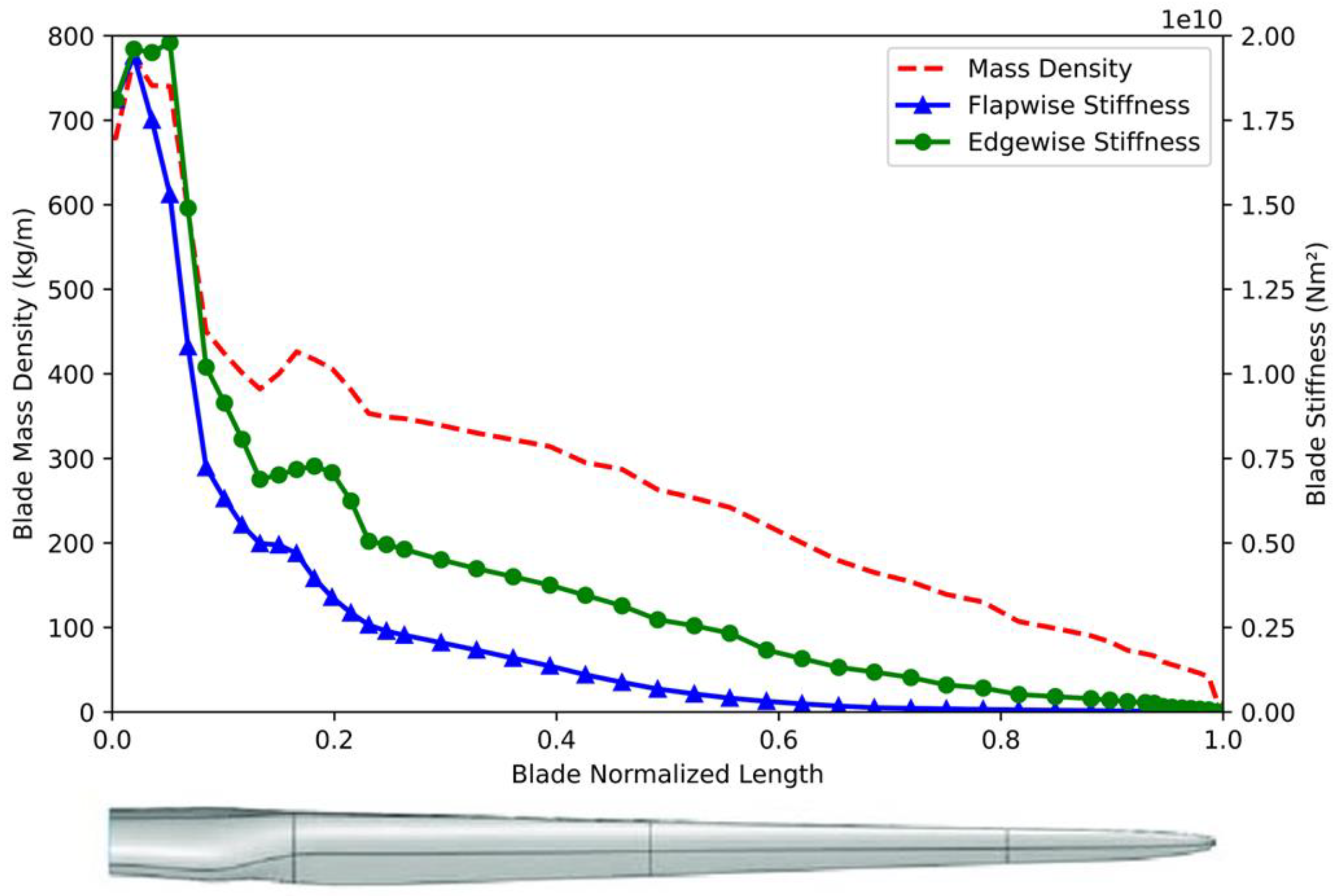
The NREL 5 MW definition report completely defines the blade’s structural properties. The blade is designed from fiberglass, and the structural properties are calculated along the blade span, which is divided into 49 sections along the 63 m span of the blade. The most effective parameters in the structural analysis are the blade mass density and blade stiffnesses in the flapwise and edgewise directions. The distributions of those properties along the span are shown in Figure 1.

To generate the datasets, aeroelastic simulations are performed on the OpenFAST simulation tool on the onshore configuration of the turbine. It uses deterministic models to calculate the aerodynamic loads and structural behavior, coupling between them for an aeroelastic analysis.

Three different wind fields are generated using the TurbSim open-source tool [25] developed by NREL for the turbulence classes A, B, and C according to the International Electrotechnical Committee standard IEC 61400-1 [26], denoting high, medium, and low turbulence intensities, respectively. TurbSim generates the wind fields based on stochastic models in the frequency domain to produce a binary wind field that covers the rotor area and shows velocities in the directions of downwind facing the rotor and crosswind and vertical wind components in the rotor plane. The Kaimal spectral model was chosen to generate the wind field since it gives better accuracy in modeling atmospheric turbulence [27]. The Kaimal model is shown in Equation (1) [28]

$${\displaystyle \frac{n{S}_u\left(n\right)}{{\sigma }_u^2}}={\displaystyle \frac{4n{L}_u/\overline{U}}{{(1+6n{L}_u/\overline{U})}^{5/3}}}$$

(1)

where n is the frequency, S_u(n) is the spectral density function, σ_u is the standard deviation of the longitudinal wind speed component, $\overline{U}$ is the mean wind speed, and L_u is a length scale that varies based on the surface roughness and the altitude.

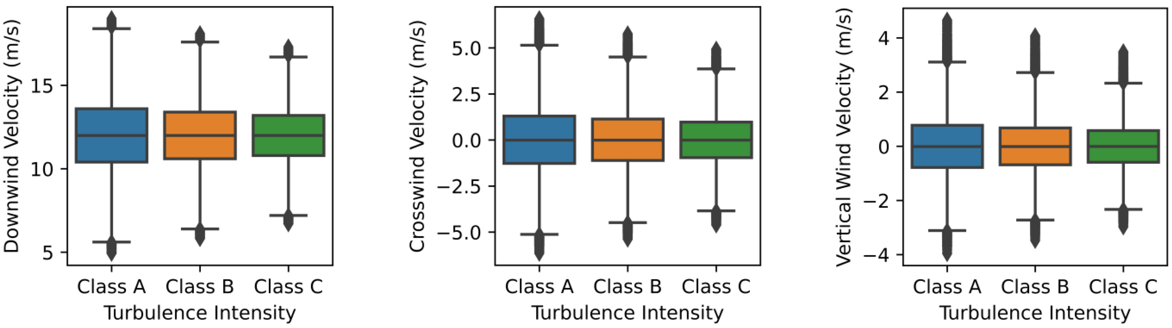
The mean wind speed chosen is 12 m/s, which is slightly above the turbine’s rated wind speed to activate the pitch control of the blade. The difference in turbulence classes does not change the mean value; it does, however, change the standard deviation and variation of wind speeds around the mean value. This is shown in Figure 2, where the quartiles of the generated wind speeds in the three directions are shown for the three turbulence classes.

The main control systems defined in the NREL 5 MW definition report are a variable speed controller for the generator-torque control system and a blade pitch-to-feather controller for the blade’s collective pitch control. Both controllers take the generator wind speed as an input to the system to produce a control action. The generator speeds are filtered using a low-pass filter with a single pole to eliminate high excitations in the generator speed. A classical proportional (P) controller is used for the variable speed control, while a proportional-integral-differential (PID) controller is used for the pitch control. The gains of each controller are calculated based on the region of operation in the turbine’s power curve and the generator speed. A complete explanation of controller gains calculations is provided in full detail in the definition report [24].

In this work, the main objective is to utilize artificial intelligence capabilities to predict blade dynamics. Hence, the simulations were run for the benchmark simulation files provided by OpenFAST, utilizing the controllers already provided by NREL. This is also useful to ensure the accuracy of the dataset, which will be used later for training the ML models. The only change performed in this work was in the turbulent wind fields used as inflow wind conditions.

The simulations are run for 20 physical minutes for each turbulent wind field, with a small time-step of 0.0063 s, resulting in 192,001 entries for each dataset. The main features of the dataset are the wind velocities in three directions in m/s, blade azimuth angle in degrees, blade pitch angle in degrees, rotor and generator speeds in rpm, and yaw deflection angle in radians. The output columns include the blade tip deflections for the flapwise and edgewise directions in m and the blade root shear force in flapwise and edgewise directions in kN. The datasets have a total of 12 columns, including the features and the outputs.

2.2. Exploratory Data Analysis

The three datasets were analyzed collectively to observe the relationships among the features and the outputs. The original datasets contained 192,001 entries for each turbulence class. The pitch control was only activated when the generator speed exceeded the rated value of 12.1 rpm. Other than that, the blade pitch angle was set to zero. To examine the pitch angle as a key feature in the ML models, the values of zero pitch angle were eliminated from the datasets, resulting in a reduction in the entries of all datasets to 107,918, 110,186, and 113,712 entries for turbulence classes A, B, and C, respectively.

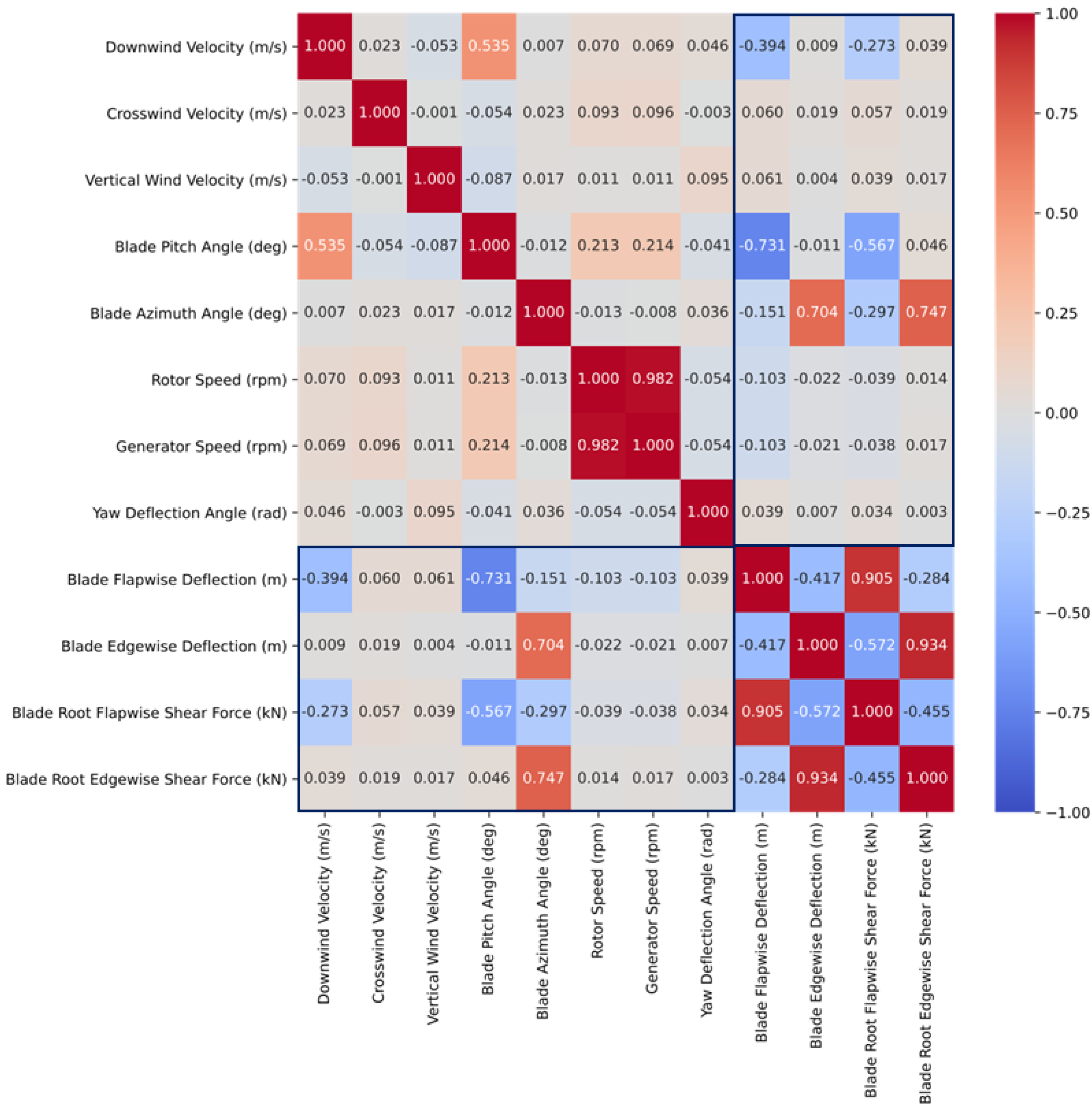
After reducing the datasets, they were all concatenated into one large dataset with 331,816 entries for data analysis. The correlation between features and outputs was calculated using the Pearson correlation method to check for a linear relationship among them. The formula used to calculate the Pearson correlation is shown in Equation (2) [29]. Figure 3 shows the Pearson correlation between the features and the outputs

$$r={\displaystyle \frac{n\sum xy-\sum x\sum y}{\sqrt{\left[n\sum x^2-{\left(\sum x\right)}^2\right]\left[n\sum y^2-{\left(\sum y\right)}^2\right]}}}$$

(2)

where r is the correlation coefficient and x and y are the independent and dependent variables, respectively. This formula estimates the correlation between each pair of variables, whether between the input features to check for multicollinearity or between the input features and the desired outputs to check for linear relationships.

A key observation from the figure is that the flapwise outputs depend inversely on the downwind velocity and the blade pitch angle. As the downwind velocity increases, the rotational speed of the rotor increases, resulting in a centrifugal force that reduces the blade deflections and forces in the flapwise direction. Blade pitch angle also reduces the force component normal to the rotor plane on the blade after it has been rotated, reducing the flapwise outputs. In the edgewise direction, the blade azimuth angle plays a significant role in the output value, which is expected since it affects the direction of gravitational loads to be in favor of or against the deflections and shear loads on the blade. Another key observation is the high correlation between the rotor and generator speeds with a value of 0.98. To avoid multicollinearity, one of the two values should be removed. The generator speed was chosen to be removed since it has a slightly lower correlation with the outputs.

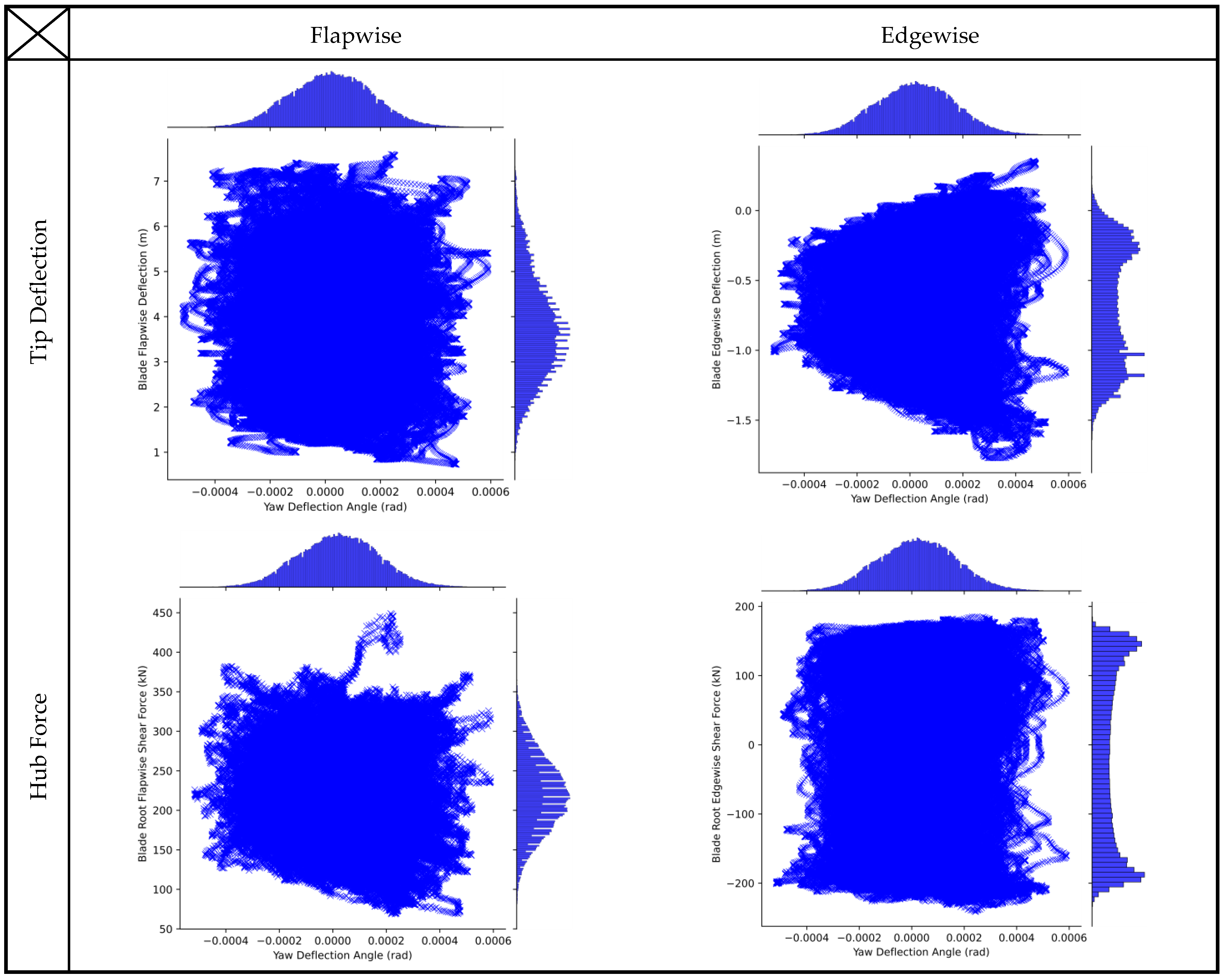
Pearson correlations could not capture the nonlinear relationship between the features and the outputs. Spearman and Kendall Tau’s correlations did not capture the relationships either. However, further exploration of the data has shown a non-linear relationship that cannot be shown using correlations. For instance, the yaw misalignment angle with the lowest correlation amongst the control parameters when plotted against the outputs has shown a dependence between their values. Figure 4 shows the effect of the yaw misalignment angle on the outputs.

Figure 4 shows the direct relationships between the yaw deflection angle and the four desired outputs. The scatter plot containing 331,816 points may be unclear to show a direct relationship between the mentioned variables. However, the scattering of the points all over the graph shows that there is a dependency between the yaw deflection and the outputs. This is emphasized by the histograms on the upper and right spines which also show a direct relationship with the flapwise direction outputs and an inverse relationship with the edgewise outputs. Noting the signs of the values, the peaks in the variables’ distribution show an increase in the values of the flapwise outputs with the increase in the yaw deflection, whether in the positive or negative senses. They also show that the outputs in the edgewise direction increase when the yaw deflection angle decreases and vice versa. The correlation alone is an indication of the suitability of linear ML models to predict the output based on the features; however, other ML models can capture the nonlinear relationships; hence, the decision was to keep all features even if the correlation is not high and try to train nonlinear and ensemble models on the data.

2.3. Machine Learning Models

The datasets are then used to train different regression ML models, including linear, nonlinear, and ensemble models. The models learn from historical data by training on a subset of the dataset, while the remainder of the dataset is used to test the model performance in predicting the outputs. The result is a model that minimizes the error between the actual and the predicted outputs.

Different quality metrics are used to assess the quality of each model for each turbulence class. The major quality metrics that were used are as follows:

• Coefficient of determination (R²):

It is a measure of the accuracy of the model. It has values between 0 and 1, with 0 meaning the model cannot predict the output and 1 meaning the model can predict the output with 100% accuracy. It can also be considered as the square of the variance and is calculated in terms of the residuals and total sum of squares. The formula for calculating R² is shown in Equation (3)

$$R^2=1-{\displaystyle \frac{\sum _{i=1}^n{(y_i-{\widehat{y}}_i)}^2}{\sum _{i=1}^n{(y_i-{\overline{y}}_i)}^2}}$$

(3)

where n is the number of entries, $y_i$ is the actual output, ${\widehat{y}}_i$ is the predicted output, and ${\overline{y}}_i$ is the mean value of the actual output.

• Root mean square error (RMSE):

It is a powerful quality metric that punishes the errors by squaring them and then taking the square root so it would be comparable to the mean value of the actual output. A higher RMSE means a higher offset of the predicted value than the actual output. The formula for calculating RMSE is shown in Equation (4).

$$RMSE=\sqrt{{\displaystyle \frac{1}{n}}(\sum _{i=1}^n{(y_i-{\widehat{y}}_i)}^2)}$$

(4)

In addition to R² and RMSE, other quality metrics were also used to evaluate the performance of each ML model. Those metrics include the mean absolute error, maximum error, training time, and normality of the residuals.

3. Results and Discussion

After analyzing the dataset, the ML models were trained on the data to generate prediction models and quality metrics were used to assess the different models. The other objective of this work is to test the generalization of the ML to be used regardless of flow conditions. For that purpose, the datasets were split again into three datasets for the different turbulence classes. The approach introduced here is to train the model on a single dataset and then use that model to predict the outputs in the other two datasets.

Before testing this generalization, 10 different ML models were trained and tested for each turbulence class dataset to determine the highest accuracy model. The highest accuracy model was then chosen to proceed with the generalization test. A summary of the models’ quality metrics, namely R², RMSE, and training time (TT) in seconds, is shown in

Table 2. Quality metrics of the ML models for the three turbulence classes.

Regression Model	Output	Turbulence Class
		Class A			Class B			Class C
		R2	RMSE	TT (s)	R2	RMSE	TT (s)	R2	RMSE	TT (s)
Linear	FW Def	0.582	0.752	0.015	0.595	0.701	0.000	0.607	0.646	0.000
	EW Def	0.492	0.299	0.000	0.510	0.289	0.015	0.526	0.278	0.015
	FW F	0.426	37.60	0.015	0.451	34.424	0.015	0.484	30.818	0.000
	EW F	0.600	79.123	0.015	0.597	79.278	0.000	0.604	78.690	0.000
Lasso	FW Def	0.576	0.757	0.000	0.587	0.708	0.031	0.598	0.654	0.000
	EW Def	0.491	0.300	0.031	0.509	0.289	0.015	0.522	0.279	0.000
	FW F	0.426	37.611	0.015	0.451	34.427	0.046	0.484	30.827	0.109
	EW F	0.600	79.118	0.000	0.596	79.330	0.015	0.603	78.734	0.031
Ridge	FW Def	0.582	0.752	0.046	0.594	0.701	0.000	0.607	0.646	0.000
	EW Def	0.492	0.299	0.031	0.510	0.289	0.046	0.525	0.279	0.015
	FW F	0.426	37.608	0.0468	0.451	34.427	0.000	0.484	30.827	0.015
	EW F	0.600	79.116	0.015	0.596	79.332	0.015	0.603	78.734	0.000
Elastic Net	FW Def	0.577	0.756	0.031	0.588	0.707	0.015	0.599	0.653	0.046
	EW Def	0.491	0.300	0.015	0.509	0.289	0.000	0.522	0.279	0.000
	FW F	0.424	37.659	0.000	0.449	34.490	0.015	0.482	30.878	0.062
	EW F	0.600	79.121	0.000	0.596	79.330	0.031	0.603	78.735	0.000
Non-linear	FW Def	0.730	0.604	0.218	0.748	0.553	0.171	0.770	0.494	0.156
	EW Def	0.564	0.277	0.218	0.576	0.269	0.187	0.585	0.260	0.109
	FW F	0.574	32.383	0.265	0.590	29.743	0.156	0.626	26.250	0.296
	EW F	0.604	78.683	0.046	0.600	78.994	0.062	0.608	78.218	0.140
Neural Network	FW Def	0.682	0.655	3.843	0.773	0.525	1.312	0.805	0.455	5.000
	EW Def	0.881	0.144	3.890	0.875	0.145	5.250	0.905	0.124	3.296
	FW F	0.839	19.920	648.234	0.851	17.940	772.734	0.813	18.533	408.078
	EW F	0.996	7.570	161.015	0.996	7.031	210.843	0.997	5.778	194.812
Decision Tree	FW Def	0.967	0.208	0.296	0.968	0.196	0.359	0.966	0.188	0.125
	EW Def	0.977	0.063	0.375	0.979	0.058	0.406	0.982	0.052	0.093
	FW F	0.948	11.229	0.281	0.949	10.457	0.375	0.943	10.237	0.156
	EW F	0.997	5.912	0.265	0.998	5.421	0.125	0.998	4.805	0.171
Random Forest	FW Def	0.984	0.144	19.562	0.983	0.139	16.343	0.984	0.130	4.406
	EW Def	0.986	0.049	18.656	0.988	0.045	16.578	0.989	0.042	4.343
	FW F	0.975	7.817	17.562	0.974	7.487	5.750	0.970	7.409	5.062
	EW F	0.998	4.890	18.750	0.998	4.440	4.125	0.999	3.952	21.703
Adaptive Boosting	FW Def	0.719	0.616	4.109	0.772	0.525	3.390	0.779	0.484	0.828
	EW Def	0.912	0.124	3.859	0.924	0.113	3.046	0.940	0.098	1.453
	FW F	0.667	28.615	3.921	0.685	26.057	3.250	0.701	23.477	1.125
	EW F	0.976	19.351	3.078	0.974	19.922	1.109	0.970	21.605	1.234
Gradient Boosting	FW Def	0.808	0.509	7.734	0.825	0.461	6.750	0.845	0.405	3.078
	EW Def	0.934	0.107	7.421	0.946	0.095	6.125	0.958	0.082	1.578
	FW F	0.724	26.074	6.406	0.757	22.905	1.781	0.785	19.901	1.875
	EW F	0.995	8.785	6.625	0.995	8.125	1.859	0.996	7.310	8.750

. The four outputs that are used for predictions are the blade tip deflections in the flapwise and edgewise directions denoted by FW Def and EW Def, respectively, and the blade root shear forces in the flapwise and edgewise directions denoted by FW F and EW F, respectively.

The linear models show almost identical results, with prediction accuracies ranging between 40 and 60%. Although the training time is the least among all other ML models, the prediction accuracy is unsatisfactory and cannot be trusted for reliable predictions of the output measures.

Adding some nonlinearity to train the data using a second-order polynomial model has slightly improved the prediction accuracies to be within the range of 56 to 77%, yet these accuracies are not sufficient. More improvements should be made to produce a reliable regression model. The neural network model, which utilizes the deep neural multilayer perceptron (MLP) method using the Scikit-learn library in Python, gives an initial judgment on the deep learning capabilities on the dataset before further investigating it in more detail. The preliminary results are not promising except for the edgewise shear force predictions. In addition, the training time for the blade root shear force outputs is much higher compared to the other ML models.

Finally, the ensemble models show the highest accuracy among all other models for most of the outputs and turbulence classes. For all outputs, decision trees and random forests give the best performance and the highest prediction accuracy. The decision tree model’s accuracy is slightly lower than the random forest, however, the training time is much shorter.

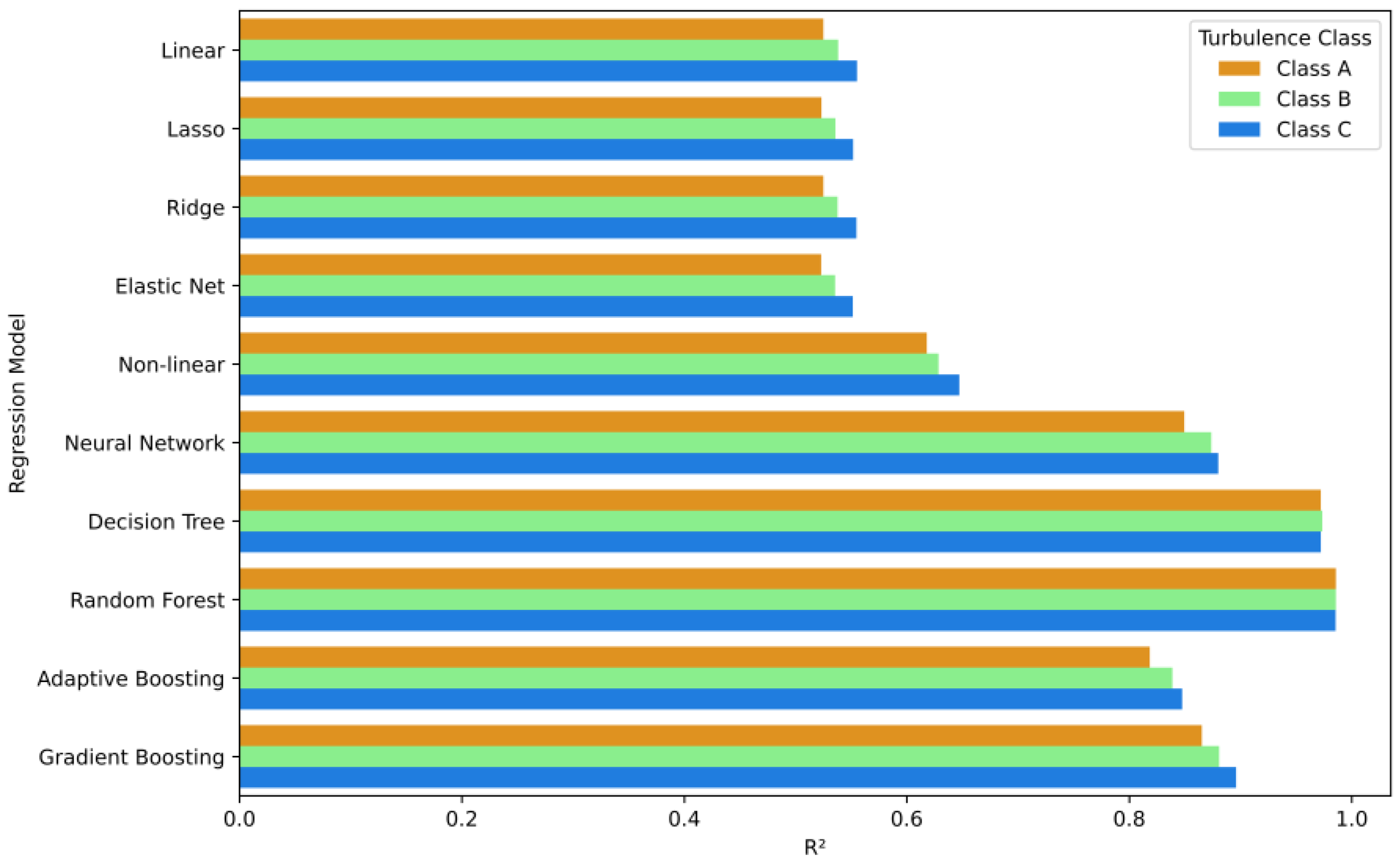
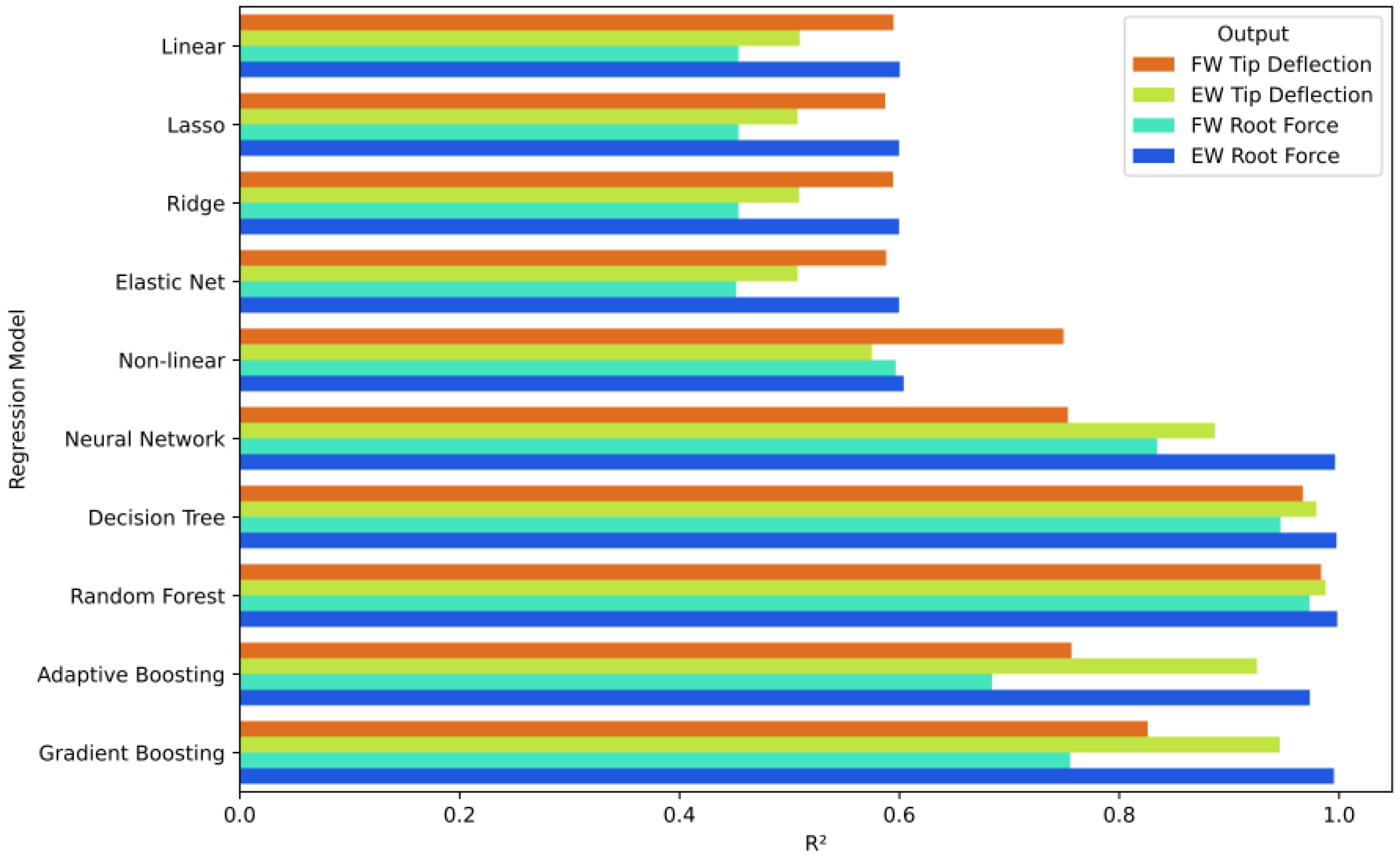
Since the models are further investigated for possible generalization, prediction accuracy is a more critical factor to consider than the computational cost. To emphasize the quality of the models before generalization, the coefficient of determination aggregate mean value with all turbulence classes and outputs are visually shown in Figure 5 and Figure 6, respectively.

The random forest model is the most stable in terms of prediction accuracy. It has almost the same R² value for all turbulence classes and outputs. The decision tree model also shows stability but with slightly less prediction accuracy. The other models show variations among the same output for different turbulence classes and vice versa. This indicates that the random forest model is the most suitable one to test for generalization.

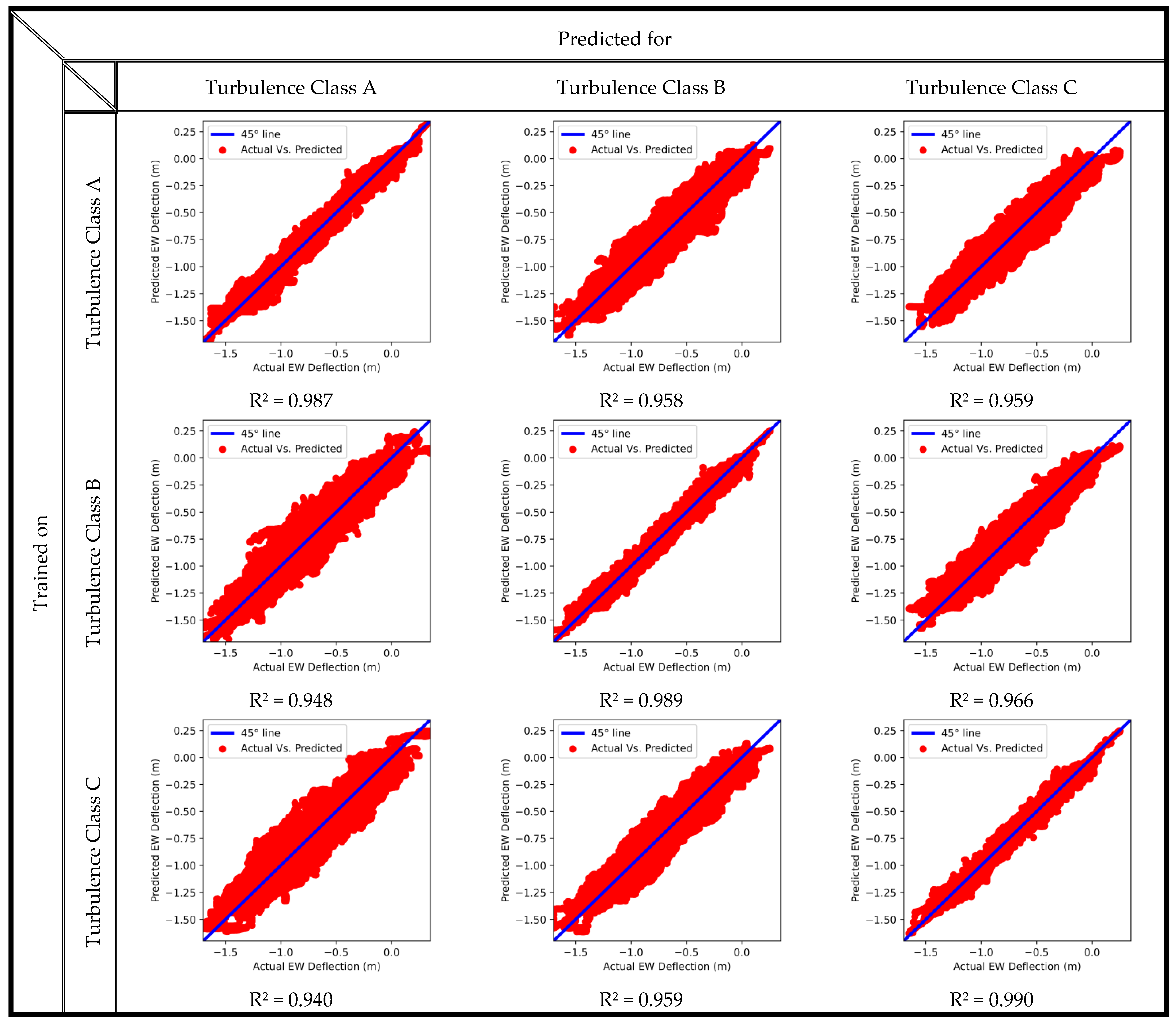
To achieve this, a random forest model is retrained on 70% of the data from a single dataset corresponding to only one turbulence class. The trained model is then tested to predict the outputs of the other two turbulence classes. This process is repeated thrice per output, once for each turbulence class. The results are shown for the blade tip deflections in the flapwise and edgewise directions. Figure 7 shows the random forest generalization results for the blade tip flapwise deflection.

On the diagonal, the prediction results are shown for the random forest model on the turbulence class on which it has been trained. The accuracies of the models are above 98%, which is satisfactory and shows the high performance of random forests. Off diagonal, the model predicts the turbulence classes for which it has not been trained. The accuracies range between 79% and 85%, which is not entirely effective. However, it can show good preliminary results in predicting the flap’s deflections under any inflow condition. It is also noteworthy that the model trained on turbulence class B shows equally accurate predictions for turbulence classes A and C. This is because class B represents medium turbulence, so it is halfway between the higher turbulence A and the lower turbulence C. This leads to the recommendation of training the model on the intermediate flow conditions in order to generalize it to other flow conditions.

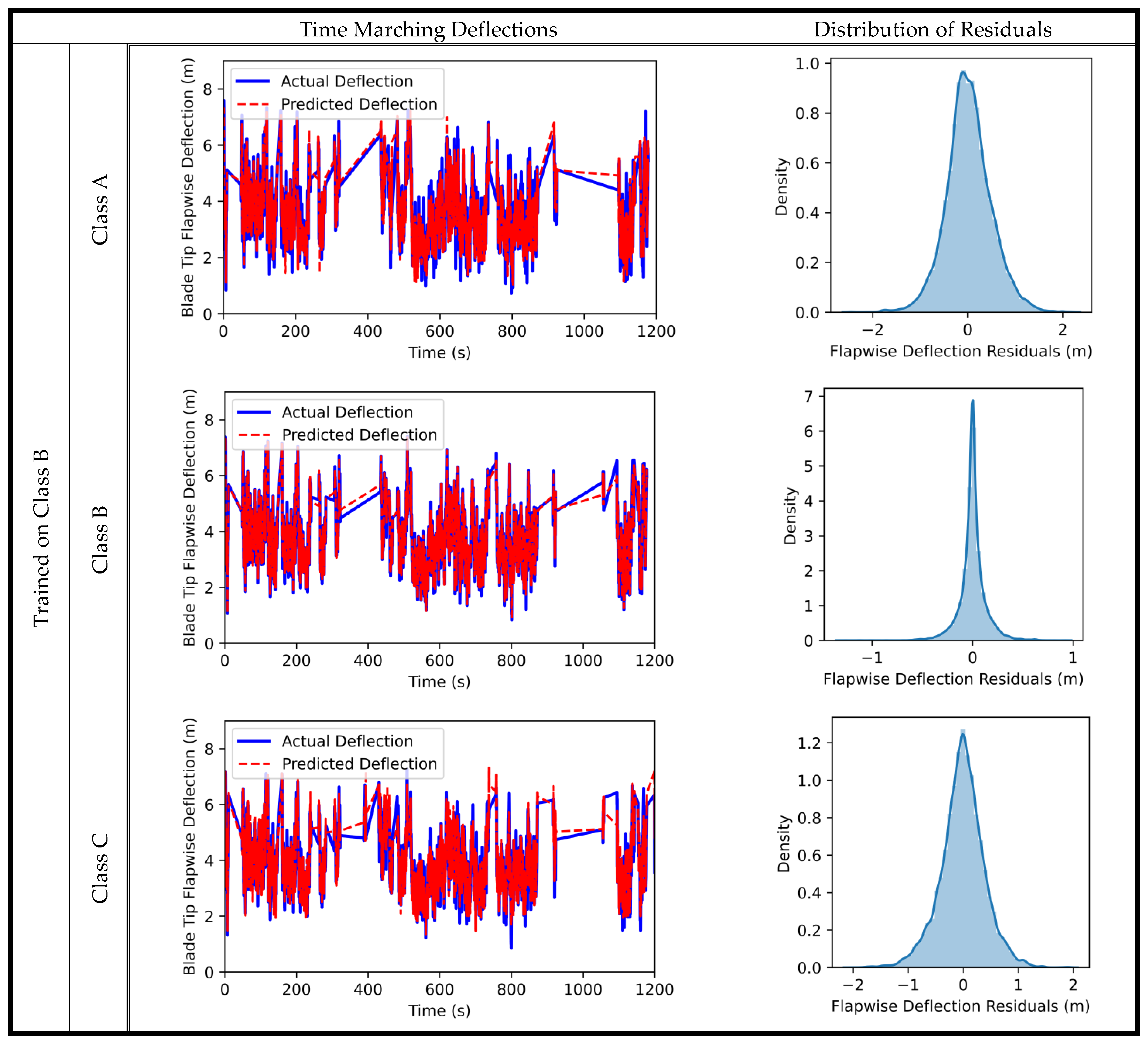
The results for the model trained on class B turbulence are plotted against time to observe the model’s performance with other turbulence classes. Also, the normality of the residuals, which is a key quality metric, is checked for that model. The time marching actual and predicted deflections of the blade tip in the flapwise direction and the residual distributions are shown only for the model trained on class B in Figure 8. The results of the models trained on classes A and C are shown in Appendix A.

The predicted deflections follow the actual ones almost perfectly for the turbulence class B on which it has been trained. This is also represented in the normality of residuals; most of the residuals are distributed around the zero value, which indicates that the prediction errors are minimal. For the other two turbulence classes, the model can still follow the deflection trend and predict the output with satisfactory accuracy. The predictions in little occurrences under or overestimate the deflections; however, these results can be used for preliminary analyses.

The process is repeated for edgewise deflections. The model is trained on each turbulence class and is used to predict its outputs and the outputs of the other two classes. The predicted values are plotted against the actual outputs and are shown in Figure 9.

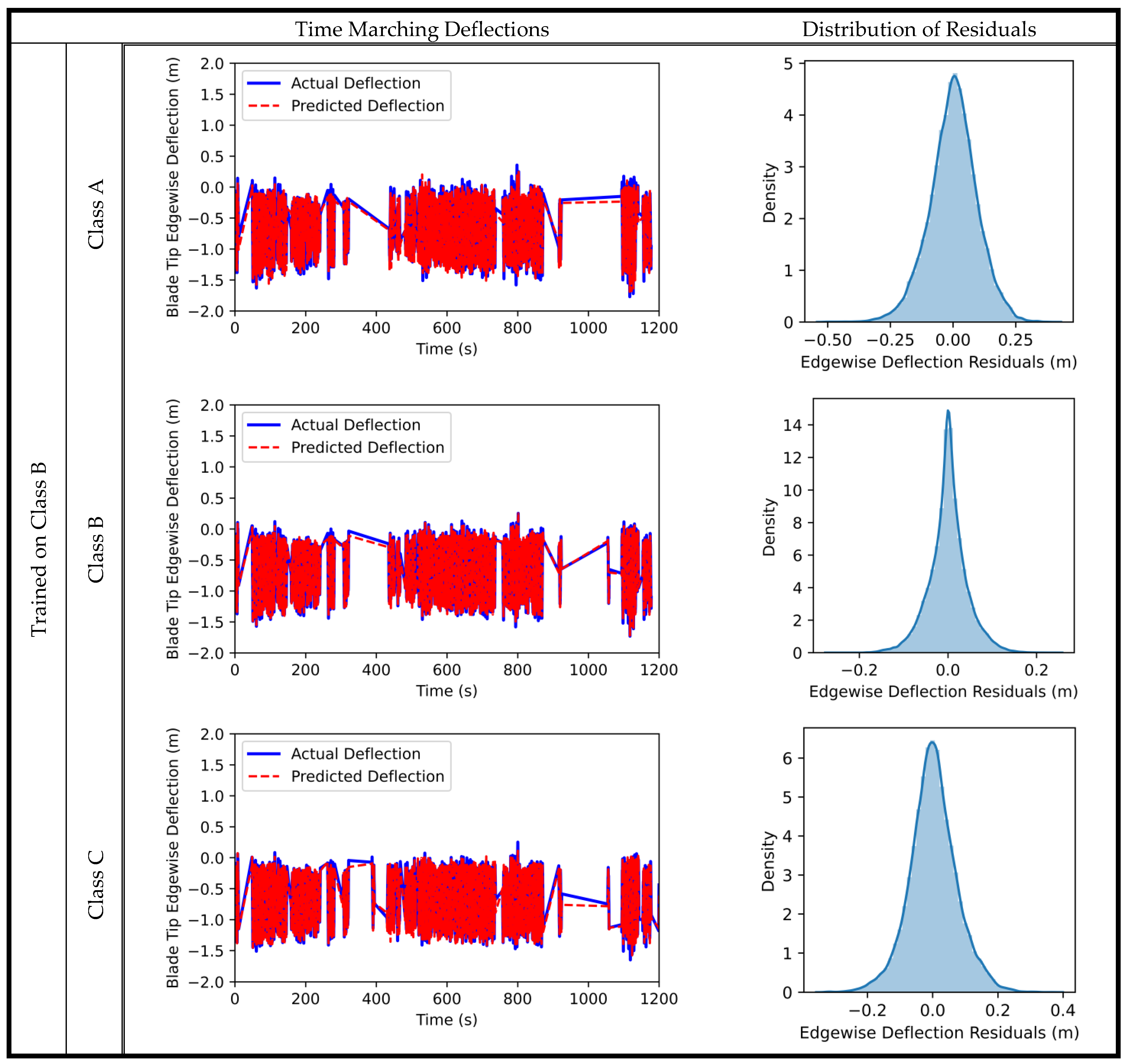
In the edgewise direction, the model performs with higher accuracy. The accuracy of predictions is above 94%, even for the datasets the model has not been trained on. This high accuracy gives more confidence in generalizing the random forest model in the edgewise structural dynamics outputs. A model trained on a single dataset can be used with high confidence for any inflow conditions. To further examine the accuracy, the time marching deflections are plotted again for turbulence class B, but in the edgewise direction. The residual distributions are also shown in Figure 10. The results for models trained on classes A and C are shown in Appendix A.

The model follows the actual output almost identically for all turbulence classes, although it has been trained on one class only. The results show slightly higher accuracy for turbulence class B that it has been trained for; however, the results for the other two classes are accurate and could be used to estimate edgewise deflections subject to any inflow conditions.

As a general observation, the generalization of the random forest regression model is more effective in the edgewise direction compared to the flapwise. This could result from the higher blade stiffness in the edgewise direction so that the deflections are within a limited range, and the model can predict it easily. Another reason is that the blade azimuth position plays a significant role in the edgewise deflections, according to the Pearson correlations in Figure 3. The blade deflects depending on its position on the rotor plane rather than the inflow conditions.

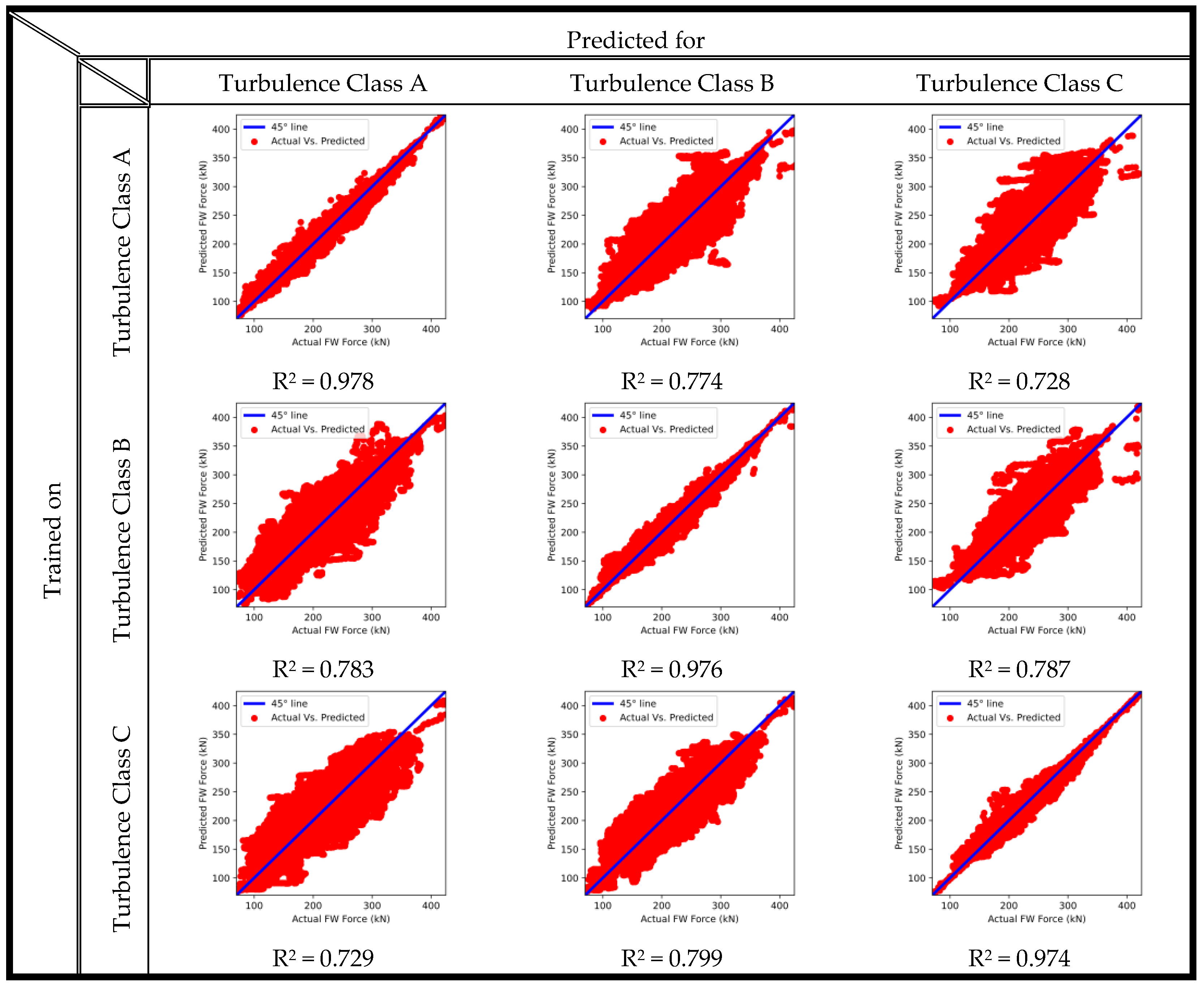
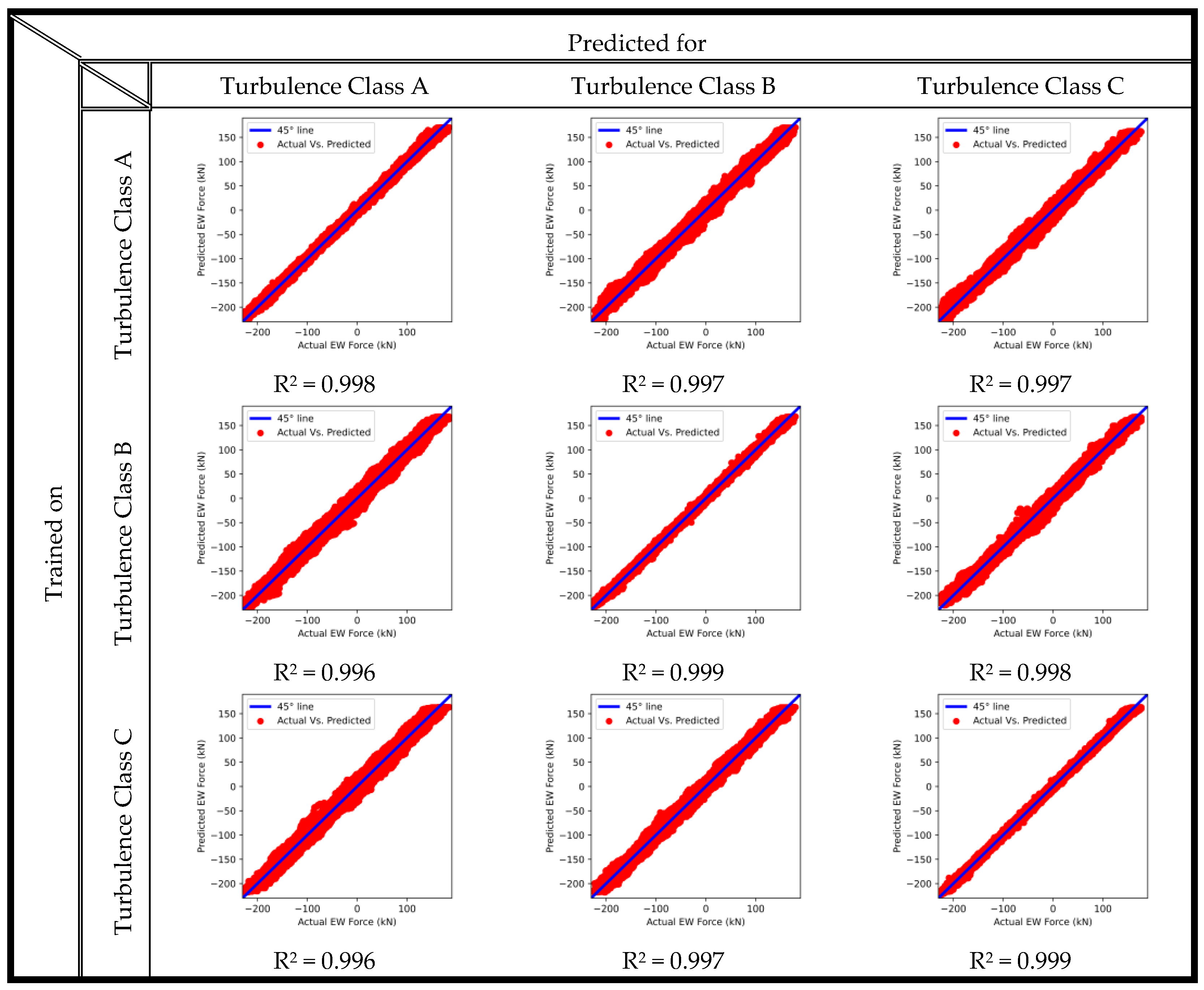
The blade root shear forces are also very important outputs to be predicted for the structural design phase. The random forest model is tested for generalization among different inflow conditions for the flapwise and edgewise shear forces. To avoid increasing the length of this paper, the results of the generalization of the random forest model are shown in Appendix B.

The main trends in predicting the blade’s root shear forces follow the same observations of the blade’s tip deflection results. The model performs in the edgewise direction with a higher accuracy compared to the flapwise direction. The prediction accuracies in the flapwise direction shear force are between the values of 73 and 98%. Meanwhile, in the edgewise direction, the accuracies are above 99.6%.

4. Conclusions

In this work, different machine learning models were used to predict structural dynamics outputs of the NREL 5 MW turbine blade. Three benchmark datasets were generated using the OpenFAST turbine simulation tool for three different turbulence intensities. The datasets were analyzed, and the features used for predictions were the inflow wind speeds, the blade’s azimuth position, and the turbine’s control parameters.

Ten different ML models were examined for accurate predictions. The linear models’ accuracies were not satisfactory and were not reliable for further investigations. Nonlinear models, as well as neural network models, could not give the required accuracy for all the desired outputs. However, ensemble models, specifically the decision tree and random forest models, could give high accuracy for all the outputs and all turbulence classes. For instance, the random forest model could predict all outputs under all turbulence classes with accuracies over 98%.

The random forest model was chosen to proceed with generalization tests to examine whether it can predict the outputs for different inflow conditions. Each turbulence class was used to train the model to predict the four outputs: blade tip deflections and blade root shear forces in the flapwise and edgewise directions. The model was then used to predict the outputs for the two remaining datasets. The model was effective in predicting the outputs even for conditions on which it was not trained. The accuracies in the flapwise direction were not high; however, it could be used in preliminary calculations, with accuracies above 79%, which is higher than the linear models trained on their outputs.

The edgewise outputs, on the other hand, could be predicted with accuracies higher than 94% for flow conditions the model was not trained on. This indicates more confidence in generalizing the random forest model to any inflow conditions. This also shows the higher dependency of the edgewise outputs on other features not directly related to the flow conditions, precisely the azimuth position of the blade.

Further investigations to assess the quality of the model could include testing for laminar flow conditions and testing the model to predict outputs for a different utility-scale wind turbine of different sizes and capacities and different blade structural properties.